Instance-Conditioned Adaptation for Large-scale Generalization
of Neural Combinatorial Optimization

Abstract

The neural combinatorial optimization (NCO) approach has shown great potential for solving routing problems without the requirement of expert knowledge. However, existing constructive NCO methods cannot directly solve large-scale instances, which significantly limits their application prospects. To address these crucial shortcomings, this work proposes a novel Instance-Conditioned Adaptation Model (ICAM) for better large-scale generalization of neural combinatorial optimization. In particular, we design a powerful yet lightweight instance-conditioned adaptation module for the NCO model to generate better solutions for instances across different scales. In addition, we develop an efficient three-stage reinforcement learning-based training scheme that enables the model to learn cross-scale features without any labeled optimal solution. Experimental results show that our proposed method is capable of obtaining excellent results with a very fast inference time in solving Traveling Salesman Problems (TSPs) and Capacitated Vehicle Routing Problems (CVRPs) across different scales. To the best of our knowledge, our model achieves state-of-the-art performance among all RL-based constructive methods for TSP and CVRP with up to 1,000 nodes.

1 Introduction

The Vehicle Routing Problem (VRP) plays a crucial role in various logistics and delivery applications, as its solution directly affects transportation cost and service efficiency. However, efficiently solving VRPs is a challenging task due to their NP-hard nature. Over the past few decades, extensive heuristic algorithms, such as LKH3 (Helsgaun, 2017) and HGS (Vidal, 2022), have been proposed to address different VRP variants. Although these approaches have shown promising results for specific problems, the algorithm designs heavily rely on expert knowledge and a deep understanding of each problem. It is very difficult to design an efficient algorithm for a newly encountered problem in real-world applications. Moreover, their required runtime can increase exponentially as the problem size grows. As a result, these limitations greatly hinder the practical application of classical heuristic algorithms.

Over the past few years, different neural combinatorial optimization (NCO) methods have been explored to solve various problems efficiently (Bengio et al., 2021; Li et al., 2022). In this work, we focus on the constructive NCO method (also known as the end-to-end method) that builds a learning-based model to directly construct an approximate solution for a given instance without the need for expert knowledge (Vinyals et al., 2015; Kool et al., 2019; Kwon et al., 2020). In addition, constructive NCO methods usually have a faster runtime compared to classical heuristic algorithms, making them a desirable choice to tackle real-world problems with real-time requirements. Existing constructive NCO methods can be divided into two categories: supervised learning (SL)-based (Vinyals et al., 2015; Xiao et al., 2023) and reinforcement learning (RL)-based ones (Nazari et al., 2018; Bello et al., 2016). The SL-based method requires a lot of problem instances with labels (i.e., the optimal solutions of these instances) as its training data. However, obtaining sufficient optimal solutions for some complex problems is unavailable, which impedes its practicality. RL-based methods learn NCO models by interacting with the environment without requiring labeled data. Nevertheless, due to memory and computational constraints, it is unrealistic to train the RL-based NCO model directly on large-scale problem instances.

Current RL-based NCO methods typically train the model on small-scale instances (e.g., with $100$ nodes) and then attempt to generalize it to larger-scale instances (e.g., with more than $1,000$ nodes) (Kool et al., 2019; Kwon et al., 2020). Although these models demonstrate good performance on instances of similar scales to the ones they were trained on, they struggle to generate reasonable good solutions for instances with much larger scales. Recently, two different types of attempts have been explored to address the crucial limitation of RL-based NCO on large-scale generalization. The first one is to perform an extra search procedure on model inference to improve the quality of solution over greedy generation (Hottung et al., 2022; Choo et al., 2022). However, this approach typically requires expert-designed search strategies and can be time-consuming when dealing with large-scale problems. The second approach is to train the model on instances of varying scales (Khalil et al., 2017; Cao et al., 2021). The challenge of this approach lies in effectively learning cross-scale features from these varying-scale training data to enhance the model’s generalization performance.

Some recent works reveal that incorporating auxiliary information (e.g., the scales of the training instances) in training can improve the model’s convergence efficiency and generalization performance. However, these methods incorporate auxiliary information into the decoding phase without including the encoding phase. Although these methods can improve the inference efficiency, the model fails to be deeply aware of the auxiliary information, resulting in unsatisfactory generalization performance on large-scale problem instances. In this work, we propose a powerful Instance-Conditioned Adaptation Model (ICAM) to improve the large-scale generalization performance for RL-based NCO. Our contributions can be summarized as follows:

• We design a novel and powerful instance-conditioned adaptation module for RL-based NCO to efficiently leverage the instance-conditioned information (e.g., instance scale and distance between each node pair) to generate better solutions across different scales. The proposed module is lightweight with low computational complexity, which can further facilitate training on instances with larger scales.

• We develop a three-stage RL-based training scheme across instances with different scales, which enables our model to learn cross-scale features without any labeled optimal solution.

• We conduct various experiments on different routing problems to demonstrate that our proposed ICAM can generate promising solutions for cross-scale instances with a very fast inference time. To the best of our knowledge, it achieves state-of-the-art performance among all RL-based constructive methods for CVRP and TSP instances with up to $1,000$ nodes.

2 Related Works

Non-conditioned NCO

Most NCO methods are trained on a fixed scale (e.g., 100 nodes). These models usually perform well on the instances with the scale they are trained on, but their performance could drop dramatically on instances with different scales (Kwon et al., 2020; Xin et al., 2020, 2021). To mitigate the poor generalization performance, an extra search procedure is usually required to find a better solution. Some widely used search methods include beam search (Joshi et al., 2019; Choo et al., 2022), Monte Carlo tree search (MCTS) (Xing & Tu, 2020; Fu et al., 2021; Qiu et al., 2022; Sun & Yang, 2023), and active search (Bello et al., 2016; Hottung et al., 2022). However, these procedures are very time-consuming, could still perform poorly on instances with quite different scales, and might require expert-designed strategies on a specific problem (e.g., MCTS for TSP). Recently, some two-stage approaches, such as divide-and-conquer (Kim et al., 2021; Hou et al., 2022) and local reconstruction (Li et al., 2021; Pan et al., 2023; Cheng et al., 2023; Ye et al., 2023), have been proposed. Although these methods have a better generalization ability, they usually require expert-designed solvers and ignore the dependency between the two stages, which makes model design difficult, especially for non-expert users.

Varying-scale Training in NCO

Directly training the NCO model on instances with different scales is another popular way to improve its generalization performance. This straightforward approach can be traced back to Khalil et al. (2017), which tries to train the model on instances with $50-100$ nodes to improve its generalization performance to instances with up to $1,200$ nodes. Furthermore, Joshi et al. (2020) systematically tests the generalization performance of NCO models by training on different TSP instances with $20-50$ nodes. Subsequently, a series of works have been developed to utilize the varying-scale training scheme to improve their own NCO models’ generalization performance (Lisicki et al., 2020; Cao et al., 2021; Manchanda et al., 2022; Gao et al., 2023; Zhou et al., 2023). Similar to the varying-size training scheme, a few SL-based NCO methods learn to construct partial solutions with various sizes during training and achieve a robust generalization performance on instances with different scales (Drakulic et al., 2023; Luo et al., 2023). Nevertheless, in real-world applications, it could be very difficult to obtain high-quality labeled solutions for SL-based model training. RL-based models also face the challenge of efficiently capturing cross-scale features from varying-scale training data, which severely hinders their generalization ability on large-scale problems.

Information-aware NCO

Recently, several works have indicated that incorporating auxiliary information (e.g., the distance between each pair of nodes) can facilitate model training and improve generalization performance. In Kim et al. (2022b), the scale-related feature is added to the decoder’s context embedding to make the model scale-aware during the decoding phase. Jin et al. (2023), Son et al. (2023) and Wang et al. (2024) use the distance to bias the compatibility calculation, thereby guiding the model toward more efficient exploration. Gao et al. (2023) employs a local policy network to catch distance and scale knowledge and integrates it into the compatibility calculation. In Li et al. (2023), the distance-related feature is utilized to adaptively refine the node embeddings so as to improve the model exploration. Overall, these methods all incorporate auxiliary information into the decoding process to improve the inference efficiency. However, this additional plugin way cannot efficiently integrate auxiliary information into the encoding of nodes and fails to enable the model to be deeply aware of the knowledge of distance and scale.

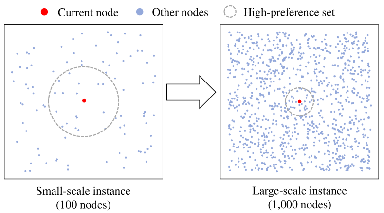
Figure 1: Node Selection Bias on Instances with Different Scales. As the scale increases, the density of nodes increases. Therefore, the model tends to select the next node from a smaller sub-region of the current node when dealing with large-scale instances compared to small-scale ones.

3 Instance-Conditioned Adaptation

3.1 Motivation and Key Idea

Each instance has some specific information that benefits the adaptability and generalization of models. By providing this instance-conditioned information, the model can better comprehend and address the problems, especially when dealing with large-scale problems. The node-to-node distances and scale are two fundamental kinds of information in routing problems, and both types of information are vital. We need to make the model aware of scale changes to improve generalization. Meanwhile, we also need to allow the model to be aware of the node-to-node distances to enhance exploration and reduce the search space, which in turn improves its training efficiency.

As the example of the two TSP instances shown in Figure 1, the two adjacent nodes in the optimal solution are normally within a specific sub-region, and the distance between them should not be too far. Likewise, the model tends to select the next node from a sub-region of the current node. For the node outside the sub-region, the farther it is from the current node, the lower the corresponding selection bias is. In addition, the nodes of instances with different scales exhibit significant variations in density. The scale is larger, and the corresponding node distribution is denser. Therefore, the model bias should vary according to the scale.

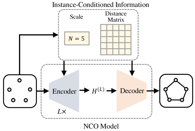
Figure 2: Intuitive Idea of Instance-Conditioned Adaptation. By providing instance-conditioned information in both the encoding and decoding processes, the model is expected to better comprehend and address problem instances.

Instance-Conditioned Adaptation Function

This work proposes to integrate the scale and node-to-node distances via an instance-conditioned adaptation function. We denote the function as $f(N,d_{ij})$, where $N$ is the scale of the problem instance, and $d_{ij}$ represents the distance between each node $i$ and each node $j$. As shown in Figure 2, the $f(N,d_{ij})$ aims to capture features related to instance scale and node-to-node distances, and feed them into the model’s encoding and decoding processes, respectively. Based on the changing instances, the model could dynamically bias the selection of nodes under the effect of $f(N,d_{ij})$, thereby making better decisions in RL-based training. To enable $f(N,d_{ij})$ to learn better features of large-scale generalization, we still need improvements in the following two aspects:

• Lightweight and Fast Model: As the RL-based training on large-scale instances consumes enormous computational time and memory, we need a more lightweight yet quick model structure so that large-scale instances can be included in the training data;

• Efficient Training Scheme: We need more efficient training schemes to accelerate model convergence, especially when training on large-scale problem instances.

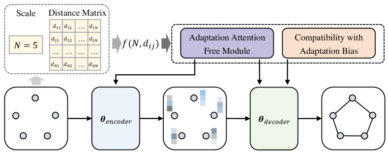
Figure 3: The Proposed ICAM. In our model, two essential types of instance-conditioned information are integrated into both the encoder and the decoder. Specifically, we utilize AAFM to replace all MHA operations in both the encoder and decoder. Moreover, we combine the adaptation function with the compatibility calculation in the decoder.

3.2 Instance-Conditioned Adaptation Model

As shown in Figure 3, the proposed ICAM also adopts the encoder-decoder structure, which is Transformer-like as many existing NCO models (Kool et al., 2019; Kim et al., 2022a; Luo et al., 2023). It is developed from a very well-known NCO model POMO (Kwon et al., 2020), and the details of POMO are provided in Appendix A.

Given an instance $X=\{\mathbf{x}_{i}\}_{i=1}^{N}$, $\mathbf{x}_{i}$ represents the features of each node (e.g., the coordinates of each city in TSP). These node features are transformed into the initial embeddings $H^{(0)}=(\mathbf{h}_{1}^{(0)},\ldots,\mathbf{h}_{N}^{(0)})$ via a linear projection. The initial embeddings pass through the $L$ attention layers to get the node embeddings $H^{(L)}=(\mathbf{h}_{1}^{(L)},\ldots,\mathbf{h}_{N}^{(L)})$. The attention layer consists of a Multi-Head Attention (MHA) sub-layer and a Feed-Forward (FF) sub-layer.

During the decoding process, the model generates a solution in an autoregressive manner. For the example of TSP, in the $t$-step construction, the context embedding is composed of the first visited node embedding and the last visited node embedding, i.e., $\mathbf{h}_{(C)}^{t}=[\mathbf{h}_{\pi_{1}}^{(L)},\mathbf{h}_{\pi_{t-1}}^{(L)}]$. The new context embedding $\hat{\mathbf{h}}_{(C)}^{t}$ is then obtained via the MHA operation on $\mathbf{h}_{(C)}^{t}$ and $H^{(L)}$. Finally, the model yields the selection probability for each unvisited node $p_{\boldsymbol{\theta}}(\pi_{t}=i\mid X,\pi_{1:t-1})$ by calculating compatibility on $\hat{\mathbf{h}}_{(C)}^{t}$ and $H^{(L)}$.

Adaptation Attention Free Module

The MHA operation is the core component of the Transformer-like NCO model. In the mode of self-attention, MHA performs a scaled dot-product attention for each head, the self-attention calculation can be written as

$$Q=XW^{Q},\quad K=XW^{K},\quad V=XW^{V},$$ (1)

$$\mathrm{Attention}(Q,K,V)=\mathrm{softmax}\left(\frac{QK^{\mathrm{T}}}{\sqrt{d_{k}}}\right)V,$$ (2)

where $X$ represents the input, $W^{Q}$, $W^{K}$, and $W^{V}$ are three learning matrices, $d_{k}$ is the dimension for $K$. The MHA incurs the primary memory usage and computational cost, which poses challenges for training on large-scale instances. Moreover, the specific design of the MHA makes it difficult to intuitively integrate the instance-conditioned information (i.e., the adaptation function $f(N,d_{ij})$).

We propose a novel module called Adaptation Attention Free Module (AAFM), as shown in Figure 4, to replace the MHA operation in both the encoder and the decoder. AAFM is based on the AFT-full operation of the Attention Free Transformer (AFT) (Zhai et al., 2021), which has lower computation and space complexity but can achieve similar performance to the MHA. The details of the AFT are provided in Appendix B. We substitute the original bias $w$ of AFT-full with our adaptation function $f(N,d_{ij})$, i.e.,

$$\mathrm{AAFM}(Q,K,V,A)=\sigma(Q)\odot\frac{\exp(A)\cdot(\exp(K)\odot V)}{\exp(A)\cdot\exp(K)},$$ (3)

where $\sigma$ is Sigmoid function, $\odot$ represents the element-wise product, and $A_{ij}=f(N,d_{ij})$ denotes the adaptation bias between node $i$ and node $j$. The detailed calculation of AAFM is shown in Figure 5.

In AAFM, instance-conditioned information is integrated in a more appropriate and ingenious manner, which enables our model to comprehend knowledge such as distance and scale more efficiently. Furthermore, our AAFM exhibits lower computation and space complexity than MHA, which could bring a more lightweight and faster model.

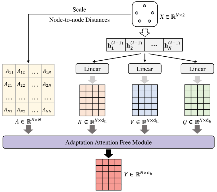
Figure 4: The Structure of AAFM. Note that in decoder, $d_{ij}$ in $A_{ij}$ is the distance between the current node and each node, and the node masking state in current step $t$ is added to $A_{ij}$ additionally.

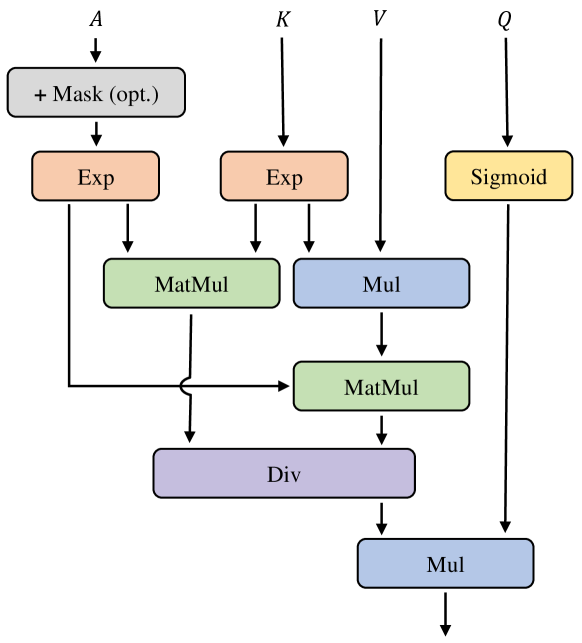
Figure 5: The Detailed Calculation Process of AAFM.

Compatibility with Adaptation Bias

We also integrate the adaptation function $f(N,d_{ij})$ into the compatibility calculation. The new compatibility, denoted as $u^{t}_{i}$, can be expressed as

$$u^{t}_{i}=\begin{cases}\xi\cdot\text{tanh}(\frac{\hat{\mathbf{h}}_{(C)}^{t}(\mathbf{h}_{i}^{(L)})^{\mathrm{T}}}{\sqrt{d_{k}}}+A_{t-1,i})&\text{if}\ i\not\in\{\pi_{1:t-1}\}\\ -\infty&\text{otherwise}\end{cases},$$ (4)

$$p_{\boldsymbol{\theta}}(\pi_{t}=i\mid X,\pi_{1:t-1})=\frac{e^{u_{i}^{t}}}{\sum_{j=1}^{N}e^{u_{j}^{t}}},$$ (5)

where $\xi$ is the clipping parameter, $\hat{\mathbf{h}}_{(C)}^{t}$ and $\mathbf{h}_{i}^{(L)}$ are calculated via AAFM instead of MHA. $A_{t-1,i}$ represents the adaptation bias between each remaining node and the current node. Finally, the probability of generating a complete solution $\mathbf{\pi}$ for instance $X$ is calculated as

$$p_{\boldsymbol{\theta}}(\mathbf{\pi}\mid X)=\prod_{t=2}^{N}p_{\boldsymbol{\theta}}(\pi_{t}\mid X,\pi_{1:t-1}).$$ (6)

By integrating the adaptation bias in the compatibility calculation, the model’s performance can be further enhanced.

3.3 Varying-scale Training Scheme

We develop a three-stage training scheme to enable the model to be aware of instance-conditioned information more effectively. We describe the three training stages as follows:

Stage 1: Warming-up on Small-scale Instances

We employ a warm-up procedure in the first stage. Initially, the model is trained for several epochs on small-scale instances. For example, we use a total of $256,000$ randomly generated TSP100 instances for each epoch in the first stage to train the model for $100$ epochs. A warm-up training can make the model more stable in the subsequent training.

Stage 2: Learning on Varying-scale Instances

In the second stage, we train the model on varying-scale instances for much longer epochs. We let the scale $N$ be randomly sampled from the discrete uniform distribution Unif([100,500]) for each batch. Considering the GPU memory constraints, we decrease the batch size with the scale increases. The loss function (denoted as $\mathcal{L}_{\mathrm{POMO}}$) used in the first and second stages is the same as in POMO. The gradient ascent with an approximation of the loss function can be written as

$$\nabla_{\theta}\mathcal{L}_{\mathrm{POMO}}(\theta)\approx\frac{1}{BN}\sum_{m=1}^{B}\sum_{i=1}^{N}G_{m,i}\nabla_{\theta}\log p_{\theta}\left(\pi^{i}\mid X_{m}\right),$$ (7)

$$G_{m,i}=R\left(\pi^{i}\mid X_{m}\right)-b^{i}(X_{m}),$$ (8)

$$b^{i}(X_{m})=\frac{1}{N}\sum_{j=1}^{N}R\left(\pi^{j}\mid X_{m}\right)\quad\text{ for all }i.$$ (9)

where $R\left(\pi^{i}\mid X_{m}\right)$ represents the return (e.g., tour length) of instance $X_{m}$ given a specific solution $\pi^{i}$. Equation 9 is a shared baseline as introduced in Kwon et al. (2020).

Stage 3: Top-$k$ Elite Training

Under the POMO structure, $N$ trajectories are constructed in parallel for each instance during training. In the third stage, we want the model to focus more on the best $k$ trajectories among all $N$ trajectories. To achieve this, we design a new loss $\mathcal{L}_{\mathrm{Top}}$, and its gradient ascent can be expressed as

$$\nabla_{\theta}\mathcal{L}_{\mathrm{Top}}(\theta)\approx\frac{1}{Bk}\sum_{m=1}^{B}\sum_{i=1}^{k}G_{m,i}\nabla_{\theta}\log p_{\theta}\left(\pi^{i}\mid X_{m}\right).$$ (10)

We combine $\mathcal{L}_{\mathrm{Top}}$ with $\mathcal{L}_{\mathrm{POMO}}$ as the joint loss in the training of the third stage, i.e.,

$$\mathcal{L}_{\mathrm{Joint}}=\mathcal{L}_{\mathrm{POMO}}+\beta\cdot\mathcal{L}_{\mathrm{Top}}.$$ (11)

where $\beta\in[0,1]$ is a coefficient balancing the original loss and the new loss.

4 Experiments

In this section, we conduct a comprehensive comparison between our proposed model and other classical and learning-based solvers using Traveling Salesman Problem (TSP) and Capacitated Vehicle Routing Problem (CVRP) instances of different scales.

Table 1: Experimental results on TSP and CVRP with uniformly distributed instances. The results marked with an asterisk (*) are directly obtained from the original papers.

	TSP100			TSP200			TSP500			TSP1000
Method	Obj.	Gap	Time	Obj.	Gap	Time	Obj.	Gap	Time	Obj.	Gap	Time
Concorde	7.7632	0.000%	34m	10.7036	0.000%	3m	16.5215	0.000%	32m	23.1199	0.000%	7.8h
LKH3	7.7632	0.000%	56m	10.7036	0.000%	4m	16.5215	0.000%	32m	23.1199	0.000%	8.2h
Att-GCN+MCTS*	7.7638	0.037%	15m	10.8139	0.884%	2m	16.9655	2.537%	6m	23.8634	3.224%	13m
DIMES AS+MCTS*	$-$	$-$	$-$	$-$	$-$	$-$	16.84	1.76%	2.15h	23.69	2.46%	4.62h
SO-mixed*	$-$	$-$	$-$	10.7873	0.636%	21.3m	16.9431	2.401%	32m	23.7656	2.800%	55.5m
DIFUSCO greedy+2-opt*	7.78	0.24%	$-$	$-$	$-$	$-$	16.80	1.49%	3.65m	23.56	1.90%	12.06m
H-TSP	$-$	$-$	$-$	$-$	$-$	$-$	17.549	6.220%	23s	24.7180	6.912%	47s
GLOP (more revisions)	7.7668	0.046%	1.9h	10.7735	0.653%	42s	16.8826	2.186%	1.6m	23.8403	3.116%	3.3m
BQ greedy	7.7903	0.349%	1.8m	10.7644	0.568%	9s	16.7165	1.180%	46s	23.6452	2.272%	1.9m
LEHD greedy	7.8080	0.577%	27s	10.7956	0.859%	2s	16.7792	1.560%	16s	23.8523	3.168%	1.6m
MDAM bs50	7.7933	0.388%	21m	10.9173	1.996%	3m	18.1843	10.065%	11m	27.8306	20.375%	44m
POMO aug$\times$8	7.7736	0.134%	1m	10.8677	1.534%	5s	20.1871	22.187%	1.1m	32.4997	40.570%	8.5m
ELG aug$\times$8	7.7988	0.458%	5.1m	10.8400	1.274%	17s	17.1821	3.998%	2.2m	24.7797	7.179%	13.7m
Pointerformer aug$\times$8	7.7759	0.163%	49s	10.7796	0.710%	11s	17.0854	3.413%	53s	24.7990	7.263%	6.4m
ICAM single trajec.	7.8328	0.897%	2s	10.8255	1.139%	<1s	16.7777	1.551%	1s	23.7976	2.931%	2s
ICAM	7.7991	0.462%	5s	10.7753	0.669%	<1s	16.6978	1.067%	4s	23.5608	1.907%	28s
ICAM aug$\times$8	7.7747	0.148%	37s	10.7385	0.326%	3s	16.6488	0.771%	38s	23.4854	1.581%	3.8m
	CVRP100			CVRP200			CVRP500			CVRP1000
Method	Obj.	Gap	Time	Obj.	Gap	Time	Obj.	Gap	Time	Obj.	Gap	Time
LKH3	15.6465	0.000%	12h	20.1726	0.000%	2.1h	37.2291	0.000%	5.5h	37.0904	0.000%	7.1h
HGS	15.5632	-0.533%	4.5h	19.9455	-1.126%	1.4h	36.5611	-1.794%	4h	36.2884	-2.162%	5.3h
GLOP-G (LKH3)	$-$	$-$	$-$	$-$	$-$	$-$	$-$	$-$	$-$	39.6507	6.903%	1.7m
BQ greedy	16.0730	2.726%	1.8m	20.7722	2.972%	10s	38.4383	3.248%	47s	39.2757	5.892%	1.9m
LEHD greedy	16.2173	3.648%	30s	20.8407	3.312%	2s	38.4125	3.178%	17s	38.9122	4.912%	1.6m
MDAM bs50	15.9924	2.211%	25m	21.0409	4.304%	3m	41.1376	10.498%	12m	47.4068	27.814%	47m
POMO aug$\times$8	15.7544	0.689%	1.2m	21.1542	4.866%	6s	44.6379	19.901%	1.2m	84.8978	128.894%	9.8m
ELG aug$\times$8	15.9973	2.242%	6.3m	20.7361	2.793%	19s	38.3413	2.987%	2.6m	39.5728	6.693%	15.6m
ICAM single trajec.	16.1868	3.453%	2s	20.7509	2.867%	<1s	37.9594	1.962%	1s	38.9709	5.070%	2s
ICAM	15.9386	1.867%	7s	20.5185	1.715%	1s	37.6040	1.007%	5s	38.4170	3.577%	35s
ICAM aug$\times$8	15.8720	1.442%	47s	20.4334	1.293%	4s	37.4858	0.689%	42s	38.2370	3.091%	4.5m

Table 2: Empirical results on CVRPLib Set-X(Uchoa et al., 2017). BKS refers to the “Best Known Solution”. The results marked with an asterisk (*) are directly obtained from the original papers.

	$N\leq 200$	200<$N\leq 500$	500<$N\leq 1000$	Total	Avg.time
	(22 instances)	(46 instances)	(32 instances)	(100 instances)
BKS	0.00%	0.00%	0.00%	0.00%	$-$
LEHD	11.35%	9.45%	17.74%	12.52%	1.58s
BQ*	$-$	$-$	$-$	9.94%	$-$
POMO	9.76%	19.12%	57.03%	29.19%	0.35s
ELG	5.50%	5.67%	5.74%	5.66%	0.61s
ICAM	5.14%	4.44%	5.17%	4.83%	0.34s

Table 3: Comparative results in the capacity setting of TAM (Hou et al., 2022) with scale $\geq$ 1000. “Time” represents the per-instance runtime. The results marked with an asterisk (*) are directly obtained from the original papers. Note that except for CVRP3000 and CVRP4000, the optimal solutions obtained using LKH3 are from the original TAM paper.

	CVRP1K			CVRP2K			CVRP3K			CVRP4K			CVRP5K
Method	Obj.	Gap	Time(s)	Obj.	Gap	Time(s)	Obj.	Gap	Time(s)	Obj.	Gap	Time(s)	Obj.	Gap	Time(s)
LKH3	46.44	0.000%	6.15	64.93	0.000%	20.29	89.90	0.000%	41.10	118.03	0.000%	80.24	175.66	0.000%	151.64
TAM-AM*	50.06	7.795%	0.76	74.31	14.446%	2.2	$-$	$-$	$-$	$-$	$-$	$-$	172.22	-1.958%	11.78
TAM-LKH3*	46.34	-0.215%	1.82	64.78	-0.231%	5.63	$-$	$-$	$-$	$-$	$-$	$-$	144.64	-17.659%	17.19
TAM-HGS*	$-$	$-$	$-$	$-$	$-$	$-$	$-$	$-$	$-$	$-$	$-$	$-$	142.83	-18.690%	30.23
GLOP-G (LKH3)	45.90	-1.163%	0.92	63.02	-2.942%	1.34	88.32	-1.758%	2.12	114.20	-3.245%	3.25	140.35	-20.101%	4.45
LEHD greedy	43.96	-5.340%	0.79	61.58	-5.159%	5.69	86.96	-3.270%	18.39	112.64	-4.567%	44.28	138.17	-21.342%	87.12
BQ greedy	44.17	-4.886%	0.55	62.59	-3.610%	1.83	88.40	-1.669%	4.65	114.15	-3.287%	11.50	139.84	-20.389%	27.63
ICAM single trajec.	43.58	-6.158%	0.02	62.38	-3.927%	0.04	89.06	-0.934%	0.10	115.09	-2.491%	0.19	140.25	-20.158%	0.28
ICAM	43.07	-7.257%	0.26	61.34	-5.529%	2.20	87.20	-3.003%	6.42	112.20	-4.939%	15.50	136.93	-22.048%	29.16

Problem Setting

For TSP and CVRP, the instances of training and testing are generated randomly, following Kool et al. (2019). For the test set, we generate $10,000$ instances for $100$-node, and $128$ instances for each of $200$-, $500$-, and $1,000$-node, respectively. Specifically, for CVRP instances of different scales, we use capacities of $50$, $80$, $100$, and $250$, respectively (Drakulic et al., 2023; Luo et al., 2023).

Model Setting

The adaptation function $f(N,d_{ij})$ should be problem-depended. For TSP and CVRP, we define it as

$$f(N,d_{ij})=-\alpha\cdot\log_{2}N\cdot d_{ij}\quad\forall i,j\in 1,\ldots,N,$$ (12)

where $\alpha$ is a learnable parameter, and it is initially set to $1$.

The embedding dimension of our model is set to $128$, and the dimension of the feed-forward layer is set to $512$. We set the number of attention layers in the encoder to $12$. The clipping parameter $\xi=50$ in Equation 4 to obtain the better training convergence (Jin et al., 2023). We train and test all experiments using a single NVIDIA GeForce RTX 3090 GPU with 24GB memory.

Training

For all models, we use Adam (Kingma & Ba, 2014) as the optimizer, initial learning rate $\eta$ is $10^{-4}$. Every epoch, we process $1,000$ batches for all problems. For each instance, $N$ different tours are always generated in parallel, each of them starting from a different city (Kwon et al., 2020). The rest of the training settings are as follows:

1. In the first stage of the process, we set different batch sizes for different problems due to memory constraints: $256$ for TSP and $128$ for CVRP. We use problem instances for TSP$100$ and CVRP$100$ to train the corresponding model for $100$ epochs. Additionally, the capacity for each CVRP instance is fixed at $50$.

2. In the second stage, the scale $N$ is randomly sampled from the discrete uniform distribution Unif([$100$,$500$]) and optimize memory usage by adjusting batch sizes according to the changed scales. For TSP, the batch size $bs=\left[160\times(\frac{100}{N})^{2}\right]$, with a training duration of 2,200 epochs. In the case of CVRP, the batch size $bs=\left[128\times(\frac{100}{N})^{2}\right]$, with a training duration of 700 epochs. Furthermore, the capacity of each batch is consistently set by random sampling from the discrete uniform distribution Unif([$50$,$100$]).

3. In the last stage, we adjust the learning rate $\eta$ to $10^{-5}$ across all models to enhance model convergence and training stability. The parameter $\beta$ and $\lambda$ are set to $0.1$ and $20$, respectively, as specified in Equation 10 and Equation 11. The training period is standardized to $200$ epochs for all models, and other settings are consistent with the second stage.

Overall, we train the TSP model for $2,500$ epochs and the CVRP model for $1,000$ epochs. For more details on model hyperparameter settings, please refer to Appendix C.

Baseline

We compare ICAM with the following methods:

1. Classical solver: Concorde (Applegate et al., 2006), LKH3 (Helsgaun, 2017) and HGS (Vidal, 2022);

2. Constructive NCO: POMO (Kwon et al., 2020), MDAM (Xin et al., 2021), ELG (Gao et al., 2023), Pointerformer (Jin et al., 2023), BQ (Drakulic et al., 2023) and LEHD (Luo et al., 2023);

3. Two-stage NCO: Att-GCN+MCTS (Fu et al., 2021), DIMES (Qiu et al., 2022), TAM (Hou et al., 2022), SO (Cheng et al., 2023), DIFUSCO (Sun & Yang, 2023), H-TSP (Pan et al., 2023) and GLOP (Ye et al., 2023).

Metrics and Inference

We use the solution lengths, optimality gaps, and total inference times to evaluate the performance of each method. Specifically, the optimality gap measures the discrepancy between the solutions generated by learning and non-learning methods and the optimal solutions, which are obtained using Concorde for TSP and LKH3 for CVRP. Note that the inference times for classical solvers, which run on a single CPU, and for learning-based methods, which utilize GPUs, are inherently different. Therefore, these times should not be directly compared.

For most NCO baseline methods, we directly execute the source code provided by the authors with default settings. We report the original results as published in corresponding papers for methods like Att-GCN+MCTS, DIMES, SO. Following the approach in Kwon et al. (2020), we report three types of results: those using a single trajectory, the best result from multiple trajectories, and results derived from instance augmentation.

Experimental Results

The experimental results on uniformly distributed instances are reported in Table 1. Our method stands out for consistently delivering superior inference performance, complemented by remarkably fast inference times, across various problem instances. Although it cannot surpass Att-GCN+MCTS on TSP100 and POMO on CVRP100, the time it consumes is significantly less. Att-GCN+MCTS takes $15$ minutes compared to our $37$ seconds. On TSP1000, our model impressively reduces the optimality gap to less than 3% in just $2$ seconds. When switching to a multi-greedy strategy, the optimality gap further narrows to 1.9% in $30$ seconds. With the instance augmentation, ICAM can achieve the optimality gap of 1.58% in less than $4$ minutes. To the best of our knowledge, for TSP and CVRP up to $1,000$ nodes, our model shows state-of-the-art performance among all RL-based constructive NCO methods.

Results on Benchmark Dataset

We further evaluate the performance of each method using the well-known benchmark datasets from CVRPLib Set-X (Uchoa et al., 2017). In these evaluations, instance augmentation is not employed for any of the methods. The detailed results are presented in Table 2, showing that our method consistently maintains the best performance. ICAM achieves the best performance across instances of all scale ranges. Among all learning-based models, ICAM has the fastest inference time. This also shows the outstanding generalization performance of ICAM. According to our knowledge, in the Set-X tests, our method has achieved the best performance to date.

Comparison on Larger-scale Instances

We also conduct experiments on instances for TSP and CVRP with larger scales, the instance augmentation is not employed for all methods due to computational efficiency. For CVRP, following  Hou et al. (2022), the capacities for instances with 1,000, 2,000, and larger scales are set at 200, 300, and 300, respectively. We perform our model on the dataset generated by the same settings. Except for CVRP3000 and CVRP4000 instances where LKH3 is used to obtain their optimal solution, the optimal solutions of other instances are from the original paper.

As shown in Table 3, on CVRP instances with scale $\geq$ 1000, our method outperforms the other methods, including GLOP with LKH3 solver and all TAM variants, on all problem instances except for CVRP3000. On CVRP3000, ICAM is slightly worse than LEHD. LEHD is an SL-based model and consumes much more solving time than ICAM. As shown in Appendix D, the superiority of ICAM is not so obvious on TSP instances with scale >$1,000$. Its performance is slightly worse than the two SL-based NCO models, BQ and LEHD. Nevertheless, on TSP$2000$ and TSP$3000$ instances, we achieve the best results in RL-based constructive methods, and on TSP$4000$ and TSP$5000$ instances, we are only slightly worse than ELG. Overall, our method still has a good large-scale generalization ability.

5 Ablation Study

ICAM vs. POMO

To improve the model’s ability to be aware of scale, we implement a varying-scale training scheme. Given that our model is an advancement over the POMO framework, we ensure a fair comparison by training a new POMO model using our training settings. The results of the two models are reported in Section E.1.

Effects of Different Stages

Our training is divided into three different stages, each contributing significantly to the overall effectiveness. The performance improvements achieved at each stage are detailed in Section E.2.

Effects of Adaptation Function

Given that we apply the adaptation function outlined in Equation 12 to both the AAFM and the subsequent compatibility calculation, we conducted three different experiments to validate the efficacy of this function. Detailed results of these experiments are available in Section E.3.

Parameter Settings in Stage 3

In the final stage, we manually adjust the $\beta$ and $k$ values as specified in Equation 10. The experimental results for two settings, involving different values, are presented in Section E.4.

Efficient Inference Strategies for Different Models

To further improve model performance, many inference strategies are developed for different NCO models. For example, BQ employs beam search, while LEHD uses the Random Re-Construct (RRC) in inference. We investigate the effects of the inference strategy on different models. The analysis is provided in Section E.5.

6 Conclusion, Limitation, and Future Work

In this work, we have proposed a novel ICAM to improve large-scale generalization for RL-based NCO. The instance-conditioned information is more effectively integrated into the model’s encoding and decoding via a powerful yet lightweight AAFM and the new compatibility calculation. In addition, we have developed a three-stage training scheme that enables the model to learn cross-scale features more efficiently. The experimental results on various TSP and CVRP instances show that ICAM achieves promising generalization abilities compared with other representative methods.

ICAM demonstrates superior performance with greedy decoding. However, we have observed its poor applicability to other complex inference strategies (e.g., RRC and beam search). In the future, we may develop a suitable inference strategy for ICAM. Moreover, the generalization performance of ICAM over differently distributed datasets should be investigated in the future.

Impact Statement

This paper presents work whose goal is to advance the field of Machine Learning. There are many potential societal consequences of our work, none which we feel must be specifically highlighted here.

Appendix A POMO Structure

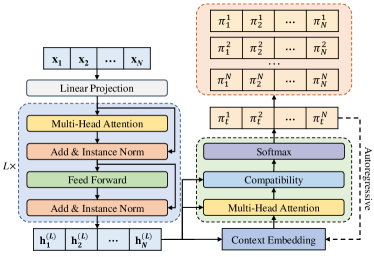
Figure 6: The Illustration of POMO Model. Note that POMO constructs $N$ trajectories for a single instance, so the decoder outputs the corresponding node selection for each trajectory at the current time step $t$.

As shown in Figure 6, POMO can be parameterized by $\boldsymbol{\theta}$, although POMO is derived from AM, it still has several differences compared to AM. The implementation of POMO is shown as follows:

Encoder

The encoder generates the embedding of each node based on the node coordinates as well as problem-specific information (e.g., user demand for CVRP), aiming at embedding the graph information of the problem into high-dimension vectors.

In the AM structure, the positional encoding is removed. And POMO disuse Layer Normalization (LN) (Ba et al., 2016), which is used by Transformer, and Batch Normalization (BN)(Ioffe & Szegedy, 2015), which is used by AM, POMO uses Instance Normalization (IN) (Ulyanov et al., 2016)

Given an instance $X=\{\mathbf{x}_{i}\}_{i=1}^{N}$, first of all, the encoder takes node features $\mathbf{x}_{i}\in\mathbb{R}^{d_{\mathrm{x}}}$ as model input, and transforms them to initial embeddings $\mathbf{\mathbf{h}}^{(0)}_{i}\in\mathbb{R}^{d_{\mathrm{h}}}$ through a linear projection, i.e., $\mathbf{h}_{i}^{(0)}={\mathbf{W}}^{\mathrm{x}}_{i}\mathbf{x}_{i}+\mathbf{b}^{\mathrm{x}}_{i}$ for $i=1,\ldots,N$. The initial embeddings $\{\mathbf{h}_{1}^{(0)},\ldots,\mathbf{h}_{N}^{(0)}\}$ pass through the $L$ attention layers in turn, and are finally transformed to the final node embeddings $H^{(L)}=(\mathbf{h}_{1}^{(L)},\ldots,\mathbf{h}_{N}^{(L)})$.

Similar to the traditional Transformer, the attention layer of POMO consists of two sub-layers: a Multi-Head Attention (MHA) sub-layer and a Feed-Forward (FF) sub-layer. Both of them use Instance Normalization and skip-connection (He et al., 2016). Let $H^{(\ell-1)}=(\mathbf{h}_{1}^{(\ell-1)},\ldots,\mathbf{h}_{N}^{(\ell-1)})$ be the input of the $\ell$-th attention layer for $\ell=1,\ldots,L$. The outputs of its MHA and FF sub-layer in terms of the $i$-th node are calculated as:

$$\hat{\mathbf{h}}_{i}^{(\ell)}=\mathrm{IN}^{(\ell)}(\mathbf{h}_{i}^{(\ell-1)}+\mathrm{MHA}^{(\ell)}(\mathbf{h}_{i}^{(\ell-1)},H^{(\ell-1)})),$$ (13)

$$\mathbf{h}_{i}^{(\ell)}=\mathrm{IN}^{(\ell)}(\mathbf{\hat{h}}_{i}^{(\ell)}+\mathrm{FF}^{(\ell)}(\mathbf{\hat{h}}_{i}^{(\ell)})),$$ (14)

where $\mathrm{IN}(\cdot)$ denotes Instance Normalization, $\mathrm{MHA}(\cdot)$ is Multi-Head Attention operation in Equation 13 (Vaswani et al., 2017), and $\mathrm{FF}(\cdot)$ in Equation 14 represents a fully connected neural network with the ReLU activation.

Decoder

Based on the node embeddings generated by the encoder, the decoder adopts autoregressive mode to step-by-step extend the existing partial solution and generate a feasible problem solution based on mask operation.

The decoder constructs the solution based on context embedding and node embeddings from the encoder step-by-step. In the latest source code provided by the authors of POMO, for each time step, POMO adopts a simpler context embedding rather than AM, and it has no graph embedding, i.e., $\bar{\mathbf{h}}^{(L)}=\frac{1}{N}\sum_{i=1}^{N}\mathbf{h}^{(L)}_{i}\in\mathbb{R}^{d_{\mathrm{h}}}$.

For the TSP, $t\in\{1,\ldots,N\}$, the context embedding $\mathbf{h}_{(C)}^{t}\in\mathbb{R}^{2\times d_{\mathbf{h}}}$ is expressed as:

$${\mathbf{h}}_{(C)}^{t}=\begin{cases}[\mathbf{h}_{\pi_{1}}^{(L)},\mathbf{h}_{\pi_{t-1}}^{(L)}]&\quad t>1\\ \mathrm{None}&\quad t=1,\end{cases}$$ (15)

where $\mathbf{h}_{\pi_{1}}^{(L)}$ is the embedding of the first visited node, in POMO, each node is considered as the first visited node, $\mathbf{h}_{\pi_{t-1}}^{(L)}$ is the embedding of the last visited node. And $[\cdot,\cdot]$ denotes the concatenation operator.

Let $\hat{\mathbf{h}}_{(C)}^{t}\in\mathbb{R}^{d_{\mathbf{h}}}$ represents the new context embedding. $\hat{\mathbf{h}}_{(C)}^{t}$ is calculated via a MHA operation:

$$\hat{\mathbf{h}}_{(C)}^{t}=\mathrm{MHA}^{(C)}(\mathbf{h}_{(C)}^{t},H^{(L)}).$$ (16)

Finally, POMO computes the compatibility $u^{t}_{i}$ using Equation 17, the output probabilities $p_{\boldsymbol{\theta}}(\pi_{t}|s,\pi_{1:t-1})$ is defined as:

$$u^{t}_{i}=\begin{cases}\xi\cdot\text{tanh}(\frac{\hat{\mathbf{h}}_{(C)}^{t}(\mathbf{h}_{i}^{(L)})^{\mathrm{T}}}{\sqrt{d_{k}}})&\text{if}\ i\not\in\{\pi_{1:t-1}\}\\ -\infty&\text{otherwise}\end{cases},$$ (17)

where $\xi=10$ is a given clipping parameter in POMO, and then the probability $p_{\boldsymbol{\theta}}(\pi_{t}=i\mid X,\pi_{1:t-1})$ of the next visiting node is obtained through Equation 5. Thereby, the probability of generating a complete solution $\mathbf{\pi}$ for instance $X$ can be calculated in Equation 6.

Training

According to Kwon et al. (2020), POMO is trained by the REINFORCE (Williams, 1992), and it uses gradient ascent with an approximation in Equation 7.

Appendix B Attention Free Transformer

According to Zhai et al. (2021), given the input $X$, AFT first transforms it to obtain $Q,K,V$ by the corresponding linear projection operation, respectively. Then, the calculation of AFT is expressed as:

$$Q=XW^{Q},\quad K=XW^{K},\quad V=XW^{V},$$ (18)

$$Y_{i}=\sigma\left(Q_{i}\right)\odot\frac{\sum_{j=1}^{N}\exp\left(K_{j}+w_{i,j}\right)\odot V_{j}}{\sum_{j=1}^{N}\exp\left(K_{j}+w_{i,j}\right)}\\$$ (19)

where $W^{Q},W^{K},W^{V}$ are three learnable matrices, $\odot$ is the element-wise product, $\sigma_{q}$ denotes the nonlinear function applied to the query $Q$, the default function is Sigmoid, $w\in\mathbb{R}^{N\times N}$ is the pair-wise position biases, and each $w_{i,j}$ is a scalar. In AFT, for every specified target position $i$, it executes a weighted average of values, and this averaged result is then integrated with the query by performing an element-wise multiplication.

The basic version of AFT outlined in Equation 19 is called AFT-full, and it is the version that we have adopted. AFT includes three additional variants: AFT-local, AFT-simple and AFT-conv. Owing to the removal of the multi-head mechanism, AFT exhibits reduced memory usage and increased speed during both the training and testing, compared to the traditional Transformer. In fact, AFT can be viewed as a specialized form of MHA, where each feature dimension is treated as an individual head. A complexity analysis comparing ”AFT-full” with these other variants is provided in Table 4. Further details are available in the related work section mentioned above.

Table 4: Complexity comparison of AFT-Full and other AFT variants. Here $N,d,s$ denote the sequence length, feature dimension, and local window size.

Model	Time	Space
Transformer	$\mathcal{O}(N^{2}d)$	$\mathcal{O}(N^{2}+Nd)$
AFT-full	$\mathcal{O}(N^{2}d)$	$\mathcal{O}(Nd)$
AFT-simple	$\mathcal{O}(Nd)$	$\mathcal{O}(Nd)$
AFT-local	$\mathcal{O}(Nsd),\ s<N$	$\mathcal{O}(Nd)$
AFT-conv	$\mathcal{O}(Nsd),\ s<N$	$\mathcal{O}(Nd)$

Appendix C Implementation Details

For the TSP and CVRP, we are adapted from the POMO model (Kwon et al., 2020), and we modify certain settings to suit our specific requirements. We remove the weight decay method because we observe that the addition of weight decay is useless for improving the model generalization performance. Note that for the CVRP model, we have implemented the gradient clipping technique, setting the max_norm parameter to $5$, to prevent the risk of exploding gradients. The rest of the settings are consistent with the original POMO model, and detailed information about the hyperparameter settings of our models can be found in Table 5.

Table 5: Model hyperparameter settings in TSP and CVRP.

	TSP	CVRP
Optimizer	Adam
Clipping parameter	50
Initial learning rate	$10^{-4}$
Learning rate of stage 3	$10^{-5}$
Weight decay	$-$
Initial $\alpha$ value	1
Loss function of stage 1 & 2	$\mathcal{L}_{\mathrm{POMO}}$
Loss function of stage 3	$\mathcal{L}_{\mathrm{Joint}}$
Parameter $\beta$ of stage 3	$0.1$
Parameter $k$ of stage 3	$20$
The number of encoder layer	$12$
Embedding dimension	$128$
Feed forward dimension	$512$
Scale of stage 1	$100$
Scale of stage 2 & 3	$[100,500]$
Batches of each epoch	$1,000$
Epochs of stage 1	$100$
Epochs of stage 3	$200$
Epochs of stage 2	$2,200$	$700$
Capacity of stage 1	$-$	$50$
Capacity of stage 2 & 3	$-$	$[50,100]$
Gradient clipping	$-$	max_norm=$5$
Batch size of stage 1	$256$	$128$
Batch size of stage 2 & 3	$\left[160\times(\frac{100}{N})^{2}\right]$	$\left[128\times(\frac{100}{N})^{2}\right]$
Total epochs	$2,500$	$1,000$

Appendix D The Results on TSP Instances with Larger-scale

Table 6: Comparative results on TSP instances with scale >1000. “Time” represents the per-instance runtime.

	TSP2K			TSP3K			TSP4K			TSP5K
Method	Obj.	Gap	Time (s)	Obj.	Gap	Time (s)	Obj.	Gap	Time (s)	Obj.	Gap	Time (s)
LKH3	32.45	0.000%	144.67	39.60	0.000%	176.13	45.66	0.000%	455.46	50.94	0.000%	710.39
LEHD greedy	34.71	6.979%	5.60	43.79	10.558%	18.66	51.79	13.428%	43.88	59.21	16.237%	85.78
BQ greedy	34.03	4.859%	1.39	42.69	7.794%	3.95	50.69	11.008%	10.50	58.12	14.106%	25.19
POMO	50.89	56.847%	4.70	65.05	64.252%	14.68	77.33	69.370%	35.12	88.28	73.308%	64.46
ELG	36.14	11.371%	6.68	45.01	13.637%	19.66	52.67	15.361%	44.84	59.47	16.758%	81.63
ICAM	34.37	5.934%	1.80	44.39	12.082%	5.62	53.00	16.075%	12.93	60.28	18.338%	24.51

As shown in Table 6, our performance is slightly worse than the two SL-based NCO models, BQ and LEHD. Nevertheless, on TSP$2000$ and TSP$3000$ instances, we achieve the best results in the RL-based constructive methods. And on TSP$4000$ and TSP$5000$ instances, we are only slightly worse than ELG. Overall, our method still has a good large-scale generalization ability. Meanwhile, this observed trend reveals an important research direction: enhancing existing adaptation bias techniques to sustain and improve the model’s performance in larger-scale TSP instances. Such advancements would enable the model to effectively tackle more extensive problem spaces while retaining its efficient solution-generation capabilities.

Appendix E Detailed Ablation Study

Please note that, unless stated otherwise, the results presented in the ablation study reflect the best result from multiple trajectories. We do not employ instance augmentation in this ablation study, and the performance on TSP instances is used as the primary criterion for evaluation.

E.1 ICAM vs. POMO

Table 7: Comparison of ICAM and POMO on TSP and CVRP instances with different scales in the same training settings.

	TSP100			TSP200			TSP500			TSP1000
Method	Obj.	Gap	Time	Obj.	Gap	Time	Obj.	Gap	Time	Obj.	Gap	Time
Concorde	7.7632	0.000%	34m	10.7036	0.000%	3m	16.5215	0.000%	32m	23.1199	0.000%	7.8h
POMO (original) single trajec.	7.8312	0.876%	2s	11.1710	4.367%	<1s	22.1027	33.781%	1s	35.1823	52.173%	2s
POMO (original)	7.7915	0.365%	8s	10.9470	2.274%	1s	20.4955	24.053%	9s	32.8566	42.114%	1.1m
POMO (original) aug$\times$8	7.7736	0.134%	1m	10.8677	1.534%	5s	20.1871	22.187%	1.1m	32.4997	40.570%	8.5m
POMO single trajec.	8.1330	4.763%	2s	11.1578	4.243%	<1s	17.3638	5.098%	1s	25.1895	8.952%	2s
POMO	7.8986	1.744%	8s	10.9080	1.910%	1s	17.0568	3.240%	9s	24.6571	6.649%	1.1m
POMO aug$\times$8	7.8179	0.704%	1m	10.8272	1.154%	5s	16.9530	2.612%	1.1m	24.5097	6.011%	8.5m
ICAM single trajec.	7.8328	0.897%	2s	10.8255	1.139%	<1s	16.7777	1.551%	1s	23.7976	2.931%	2s
ICAM	7.7991	0.462%	5s	10.7753	0.669%	<1s	16.6978	1.067%	4s	23.5608	1.907%	28s
ICAM aug$\times$8	7.7747	0.148%	37s	10.7385	0.326%	3s	16.6488	0.771%	38s	23.4854	1.581%	3.8m
	CVRP100			CVRP200			CVRP500			CVRP1000
Method	Obj.	Gap	Time	Obj.	Gap	Time	Obj.	Gap	Time	Obj.	Gap	Time
LKH3	15.6465	0.000%	12h	20.1726	0.000%	2.1h	37.2291	0.000%	5.5h	37.0904	0.000%	7.1h
POMO (original) single trajec.	16.0264	2.428%	2s	21.9590	8.856%	<1s	50.2240	34.905%	1s	150.4555	305.645%	2s
POMO (original)	15.8368	1.217%	10s	21.3529	5.851%	1s	48.2247	29.535%	10s	143.1178	285.862%	1.2m
POMO (original) aug$\times$8	15.7544	0.689%	1.2m	21.1542	4.866%	6s	44.6379	19.901%	1.2m	84.8978	128.894%	9.8m
POMO single trajec.	16.3210	4.311%	2s	20.9470	3.839%	<1s	38.2987	2.873%	1s	39.6420	6.879%	2s
POMO	16.0200	2.387%	10s	20.6380	2.307%	1s	37.8702	1.722%	10s	39.0244	5.214%	1.2m
POMO aug$\times$8	15.8575	1.348%	1.2m	20.4851	1.549%	6s	37.6902	1.238%	1.2m	38.7652	4.515%	9.8m
ICAM single trajec.	16.1868	3.453%	2s	20.7509	2.867%	<1s	37.9594	1.962%	1s	38.9709	5.070%	2s
ICAM	15.9386	1.867%	7s	20.5185	1.715%	1s	37.6040	1.007%	5s	38.4170	3.577%	35s
ICAM aug$\times$8	15.8720	1.442%	47s	20.4334	1.293%	4s	37.4858	0.689%	42s	38.2370	3.091%	4.5m

As detailed in Table 7, in our three-stage training scheme, POMO also obtains better performance on large-scale instances compared to the original model, yet it falls short of ICAM’s performance. In contrast to POMO, ICAM excels in capturing cross-scale features and perceiving instance-conditioned information. This ability notably enhances model performance in solving problems across various scales. Detailed information on the model’s performance at different stages can be found in Section E.2.

E.2 The Effects of Different Stages

Table 8: Comparison between different stages on TSP instances with different scales.

	TSP100	TSP200	TSP500	TSP1000
After stage 1	0.514%	1.856%	7.732%	12.637%
After stage 2	0.662%	0.993%	1.515%	2.716%
After stage 3	0.462%	0.669%	1.067%	1.907%

As illustrated in Table 8, after the first stage, the model performs outstanding performance with small-scale instances but underperforms when dealing with large-scale instances. After the second stage, there is a marked improvement in the ability to solve large-scale instances. By the end of the final stage, the overall performance is further improved. Notably, in our ICAM, the capability to tackle small-scale instances is not affected despite the instance scales varying during the training.

E.3 The Effects of Instance-Conditioned Adaptation Function

Table 9: The detailed ablation study on instance-conditioned adaptation function. Here AFM denotes that AAFM removes the adaptation bias, and CAB is the compatibility with the adaptation bias.

	TSP100	TSP200	TSP500	TSP1000
AFM	1.395%	2.280%	4.890%	8.872%
AFM+CAB	0.956%	1.733%	4.081%	7.090%
AAFM	0.514%	0.720%	1.135%	2.241%
AAFM+CAB	0.462%	0.669%	1.067%	1.907%

The data presented in Table 9 indicates a notable enhancement in the solving performance across various scales when instance-conditioned information, such as scale and node-to-node distances, is integrated into the model. This improvement emphasizes the importance of including detailed, fine-grained information in the model. It also highlights the critical role of explicit instance-conditioned information in improving the adaptability and generalization capabilities of RL-based models. In particular, the incorporation of richer instance-conditioned information allows the model to more effectively comprehend and address the challenges, especially in the context of large-scale problems.

E.4 Parameter Settings in Stage 3

Table 10: Comparison between different parameters in Stage 3 on TSP instances with $1,000$ nodes.

	single trajec.				no augment.
	$\beta=0$	$\beta=0.1$	$\beta=0.5$	$\beta=0.9$	$\beta=0$	$\beta=0.1$	$\beta=0.5$	$\beta=0.9$
$k=20$	2.996%	2.931%	3.423%	3.480%	2.039%	1.907%	1.859%	1.875%
$k=50$	$-$	3.060%	3.123%	3.328%	$-$	1.935%	1.892%	1.857%
$k=100$	$-$	2.979%	3.201%	3.343%	$-$	1.948%	1.899%	1.899%

As indicated in Table 10, when trained using $\mathcal{L}_{\mathrm{Joint}}$ as outlined in Equation 11, our model shows further improved performance. When using the multi-greedy search strategy, we observe no significant performance variation among different models at various $k$ values. However, increasing the $\beta$ coefficients, while yielding a marginal improvement in performance with the multi-greedy strategy, notably diminishes the solving efficiency in the single-trajectory mode. Given the challenges in generating $N$ trajectories for a single instance as the instance scale increases, we are focusing on optimizing the model effectiveness specifically in the single trajectory mode to obtain the best possible performance.

E.5 Comparison of Different Inference Strategies

As detailed in Table 11, upon attempting to replace the instance augmentation strategy with alternative inference strategies, it is observed that there is no significant improvement in the performance of our model. However, the incorporation of RRC technology into the LEHD model and the implementation of beam search technology into the BQ model both result in substantial enhancements to the performance of respective models. This highlights a crucial insight: different models require different inference strategies to optimize their performance. Consequently, it is essential to investigate more effective strategies to achieve further improvements in the performance of ICAM.

Table 11: Experimental results with different inference strategies on TSP instances.

	TSP100			TSP200			TSP500			TSP1000
Method	Obj.	Gap	Time	Obj.	Gap	Time	Obj.	Gap	Time	Obj.	Gap	Time
Concorde	7.7632	0.000%	34m	10.7036	0.000%	3m	16.5215	0.000%	32m	23.1199	0.000%	7.8h
BQ greedy	7.7903	0.349%	1.8m	10.7644	0.568%	9s	16.7165	1.180%	46s	23.6452	2.272%	1.9m
BQ bs16	7.7644	0.016%	27.5m	10.7175	0.130%	2m	16.6171	0.579%	11.9m	23.4323	1.351%	29.4m
LEHD greedy	7.8080	0.577%	27s	10.7956	0.859%	2s	16.7792	1.560%	16s	23.8523	3.168%	1.6m
LEHD RRC100	7.7640	0.010%	16m	10.7096	0.056%	1.2m	16.5784	0.344%	8.7m	23.3971	1.199%	48.6m
ICAM single trajec.	7.8328	0.897%	2s	10.8255	1.139%	<1s	16.7777	1.551%	1s	23.7976	2.931%	2s
ICAM	7.7991	0.462%	5s	10.7753	0.669%	<1s	16.6978	1.067%	4s	23.5608	1.907%	28s
ICAM RRC100	7.7950	0.409%	2.4m	10.7696	0.616%	14s	16.6886	1.012%	2.4m	23.5488	1.855%	16.8m
ICAM bs16	7.7915	0.365%	1.3m	10.7672	0.594%	14s	16.6889	1.013%	1.5m	23.5436	1.833%	10.5m
ICAM aug$\times$8	7.7747	0.148%	37s	10.7385	0.326%	3s	16.6488	0.771%	38s	23.4854	1.581%	3.8m

Appendix F Licenses for Used Resources

Table 12: List of licenses for the codes and datasets we used in this work

Resource	Type	Link	License
Concorde (Applegate et al., 2006)	Code	https://github.com/jvkersch/pyconcorde	BSD 3-Clause License
LKH3 (Helsgaun, 2017)	Code	http://webhotel4.ruc.dk/~keld/research/LKH-3/	Available for academic research use
HGS (Vidal, 2022)	Code	https://github.com/chkwon/PyHygese	MIT License
H-TSP (Pan et al., 2023)	Code	https://github.com/Learning4Optimization-HUST/H-TSP	Available for academic research use
GLOP (Ye et al., 2023)	Code	https://github.com/henry-yeh/GLOP	MIT License
POMO (Kwon et al., 2020)	Code	https://github.com/yd-kwon/POMO/tree/master/NEW_py_ver	MIT License
ELG (Gao et al., 2023)	Code	https://github.com/gaocrr/ELG	MIT License
Pointerformer (Jin et al., 2023)	Code	https://github.com/pointerformer/pointerformer	Available for academic research use
MDAM (Xin et al., 2021)	Code	https://github.com/liangxinedu/MDAM	MIT License
LEHD (Luo et al., 2023)	Code	https://github.com/CIAM-Group/NCO_code/tree/main/single_objective/LEHD	Available for any non-commercial use
BQ (Drakulic et al., 2023)	Code	https://github.com/naver/bq-nco	CC BY-NC-SA 4.0 license
CVRPLib	Dataset	http://vrp.galgos.inf.puc-rio.br/index.php/en/	Available for academic research use

We list the used existing codes and datasets in Table 12, and all of them are open-sourced resources for academic usage.

References

- Applegate et al. (2006) Applegate, D., Bixby, R., Chvatal, V., and Cook, W. Concorde tsp solver, 2006.
- Ba et al. (2016) Ba, J. L., Kiros, J. R., and Hinton, G. E. Layer normalization. arXiv preprint arXiv:1607.06450, 2016.
- Bello et al. (2016) Bello, I., Pham, H., Le, Q. V., Norouzi, M., and Bengio, S. Neural combinatorial optimization with reinforcement learning. arXiv preprint arXiv:1611.09940, 2016.
- Bengio et al. (2021) Bengio, Y., Lodi, A., and Prouvost, A. Machine learning for combinatorial optimization: a methodological tour d’horizon. European Journal of Operational Research, 290(2):405–421, 2021.
- Cao et al. (2021) Cao, Y., Sun, Z., and Sartoretti, G. Dan: Decentralized attention-based neural network for the minmax multiple traveling salesman problem. arXiv preprint arXiv:2109.04205, 2021.
- Cheng et al. (2023) Cheng, H., Zheng, H., Cong, Y., Jiang, W., and Pu, S. Select and optimize: Learning to aolve large-scale tsp instances. In International Conference on Artificial Intelligence and Statistics, pp. 1219–1231. PMLR, 2023.
- Choo et al. (2022) Choo, J., Kwon, Y.-D., Kim, J., Jae, J., Hottung, A., Tierney, K., and Gwon, Y. Simulation-guided beam search for neural combinatorial optimization. Advances in Neural Information Processing Systems, 35:8760–8772, 2022.
- Drakulic et al. (2023) Drakulic, D., Michel, S., Mai, F., Sors, A., and Andreoli, J.-M. Bq-nco: Bisimulation quotienting for efficient neural combinatorial optimization. In Thirty-seventh Conference on Neural Information Processing Systems, 2023.
- Fu et al. (2021) Fu, Z.-H., Qiu, K.-B., and Zha, H. Generalize a small pre-trained model to arbitrarily large tsp instances. In Proceedings of the AAAI Conference on Artificial Intelligence, volume 35, pp. 7474–7482, 2021.
- Gao et al. (2023) Gao, C., Shang, H., Xue, K., Li, D., and Qian, C. Towards generalizable neural solvers for vehicle routing problems via ensemble with transferrable local policy. arXiv preprint arXiv:2308.14104, 2023.
- He et al. (2016) He, K., Zhang, X., Ren, S., and Sun, J. Deep residual learning for image recognition. In Proceedings of the IEEE Conference on Computer Vision and Pattern Recognition, pp. 770–778, 2016.
- Helsgaun (2017) Helsgaun, K. An extension of the lin-kernighan-helsgaun tsp solver for constrained traveling salesman and vehicle routing problems. Roskilde: Roskilde University, 12, 2017.
- Hottung et al. (2022) Hottung, A., Kwon, Y.-D., and Tierney, K. Efficient active search for combinatorial optimization problems. In International Conference on Learning Representations, 2022.
- Hou et al. (2022) Hou, Q., Yang, J., Su, Y., Wang, X., and Deng, Y. Generalize learned heuristics to solve large-scale vehicle routing problems in real-time. In The Eleventh International Conference on Learning Representations, 2022.
- Ioffe & Szegedy (2015) Ioffe, S. and Szegedy, C. Batch normalization: Accelerating deep network training by reducing internal covariate shift. In International Conference on Machine Learning, pp. 448–456. PMLR, 2015.
- Jin et al. (2023) Jin, Y., Ding, Y., Pan, X., He, K., Zhao, L., Qin, T., Song, L., and Bian, J. Pointerformer: Deep reinforced multi-pointer transformer for the traveling salesman problem. In The Thirty-Seventh AAAI Conference on Artificial Intelligence, 2023.
- Joshi et al. (2019) Joshi, C. K., Laurent, T., and Bresson, X. An efficient graph convolutional network technique for the travelling salesman problem. arXiv preprint arXiv:1906.01227, 2019.
- Joshi et al. (2020) Joshi, C. K., Cappart, Q., Rousseau, L.-M., and Laurent, T. Learning the travelling salesperson problem requires rethinking generalization. arXiv preprint arXiv:2006.07054, 2020.
- Khalil et al. (2017) Khalil, E., Dai, H., Zhang, Y., Dilkina, B., and Song, L. Learning combinatorial optimization algorithms over graphs. Advances in Neural Information Processing Systems, 30, 2017.
- Kim et al. (2021) Kim, M., Park, J., et al. Learning collaborative policies to solve np-hard routing problems. Advances in Neural Information Processing Systems, 34:10418–10430, 2021.
- Kim et al. (2022a) Kim, M., Park, J., and Park, J. Sym-nco: Leveraging symmetricity for neural combinatorial optimization. Advances in Neural Information Processing Systems, 35:1936–1949, 2022a.
- Kim et al. (2022b) Kim, M., Son, J., Kim, H., and Park, J. Scale-conditioned adaptation for large scale combinatorial optimization. In NeurIPS 2022 Workshop on Distribution Shifts: Connecting Methods and Applications, 2022b.
- Kingma & Ba (2014) Kingma, D. P. and Ba, J. Adam: A method for stochastic optimization. arXiv preprint arXiv:1412.6980, 2014.
- Kool et al. (2019) Kool, W., van Hoof, H., and Welling, M. Attention, learn to solve routing problems! In International Conference on Learning Representations, 2019.
- Kwon et al. (2020) Kwon, Y.-D., Choo, J., Kim, B., Yoon, I., Gwon, Y., and Min, S. Pomo: Policy optimization with multiple optima for reinforcement learning. Advances in Neural Information Processing Systems, 33:21188–21198, 2020.
- Li et al. (2022) Li, B., Wu, G., He, Y., Fan, M., and Pedrycz, W. An overview and experimental study of learning-based optimization algorithms for the vehicle routing problem. IEEE/CAA Journal of Automatica Sinica, 9(7):1115–1138, 2022.
- Li et al. (2023) Li, J., Ma, Y., Cao, Z., Wu, Y., Song, W., Zhang, J., and Chee, Y. M. Learning feature embedding refiner for solving vehicle routing problems. IEEE Transactions on Neural Networks and Learning Systems, 2023.
- Li et al. (2021) Li, S., Yan, Z., and Wu, C. Learning to delegate for large-scale vehicle routing. Advances in Neural Information Processing Systems, 34:26198–26211, 2021.
- Lisicki et al. (2020) Lisicki, M., Afkanpour, A., and Taylor, G. W. Evaluating curriculum learning strategies in neural combinatorial optimization. arXiv preprint arXiv:2011.06188, 2020.
- Luo et al. (2023) Luo, F., Lin, X., Liu, F., Zhang, Q., and Wang, Z. Neural combinatorial optimization with heavy decoder: Toward large scale generalization. In Thirty-seventh Conference on Neural Information Processing Systems, 2023.
- Manchanda et al. (2022) Manchanda, S., Michel, S., Drakulic, D., and Andreoli, J.-M. On the generalization of neural combinatorial optimization heuristics. In Joint European Conference on Machine Learning and Knowledge Discovery in Databases, pp. 426–442. Springer, 2022.
- Nazari et al. (2018) Nazari, M., Oroojlooy, A., Snyder, L., and Takác, M. Reinforcement learning for solving the vehicle routing problem. Advances in neural information processing systems, 31, 2018.
- Pan et al. (2023) Pan, X., Jin, Y., Ding, Y., Feng, M., Zhao, L., Song, L., and Bian, J. H-tsp: Hierarchically solving the large-scale travelling salesman problem. In Proceedings of the AAAI Conference on Artificial Intelligence, 2023.
- Qiu et al. (2022) Qiu, R., Sun, Z., and Yang, Y. Dimes: A differentiable meta solver for combinatorial optimization problems. Advances in Neural Information Processing Systems, 35:25531–25546, 2022.
- Son et al. (2023) Son, J., Kim, M., Kim, H., and Park, J. Meta-sage: Scale meta-learning scheduled adaptation with guided exploration for mitigating scale shift on combinatorial optimization. In International Conference on Machine Learning. PMLR, 2023.
- Sun & Yang (2023) Sun, Z. and Yang, Y. Difusco: Graph-based diffusion solvers for combinatorial optimization. arXiv preprint arXiv:2302.08224, 2023.
- Uchoa et al. (2017) Uchoa, E., Pecin, D., Pessoa, A., Poggi, M., Vidal, T., and Subramanian, A. New benchmark instances for the capacitated vehicle routing problem. European Journal of Operational Research, 257(3):845–858, 2017.
- Ulyanov et al. (2016) Ulyanov, D., Vedaldi, A., and Lempitsky, V. Instance normalization: The missing ingredient for fast stylization. arXiv preprint arXiv:1607.08022, 2016.
- Vaswani et al. (2017) Vaswani, A., Shazeer, N., Parmar, N., Uszkoreit, J., Jones, L., Gomez, A. N., Kaiser, Ł., and Polosukhin, I. Attention is all you need. Advances in Neural Information Processing Systems, 30, 2017.
- Vidal (2022) Vidal, T. Hybrid genetic search for the cvrp: Open-source implementation and swap* neighborhood. Computers & Operations Research, 140:105643, 2022.
- Vinyals et al. (2015) Vinyals, O., Fortunato, M., and Jaitly, N. Pointer networks. Advances in neural information processing systems, 28, 2015.
- Wang et al. (2024) Wang, Y., Jia, Y.-H., Chen, W.-N., and Mei, Y. Distance-aware attention reshaping: Enhance generalization of neural solver for large-scale vehicle routing problems. arXiv preprint arXiv:2401.06979, 2024.
- Williams (1992) Williams, R. J. Simple statistical gradient-following algorithms for connectionist reinforcement learning. Machine learning, 8:229–256, 1992.
- Xiao et al. (2023) Xiao, Y., Wang, D., Li, B., Wang, M., Wu, X., Zhou, C., and Zhou, Y. Distilling autoregressive models to obtain high-performance non-autoregressive solvers for vehicle routing problems with faster inference speed. arXiv preprint arXiv:2312.12469, 2023.
- Xin et al. (2020) Xin, L., Song, W., Cao, Z., and Zhang, J. Step-wise deep learning models for solving routing problems. IEEE Transactions on Industrial Informatics, 17(7):4861–4871, 2020.
- Xin et al. (2021) Xin, L., Song, W., Cao, Z., and Zhang, J. Multi-decoder attention model with embedding glimpse for solving vehicle routing problems. In Proceedings of the AAAI Conference on Artificial Intelligence, volume 35, pp. 12042–12049, 2021.
- Xing & Tu (2020) Xing, Z. and Tu, S. A graph neural network assisted monte carlo tree search approach to traveling salesman problem. IEEE Access, 8:108418–108428, 2020.
- Ye et al. (2023) Ye, H., Wang, J., Liang, H., Cao, Z., Li, Y., and Li, F. Glop: Learning global partition and local construction for solving large-scale routing problems in real-time. arXiv preprint arXiv:2312.08224, 2023.
- Zhai et al. (2021) Zhai, S., Talbott, W., Srivastava, N., Huang, C., Goh, H., Zhang, R., and Susskind, J. An attention free transformer. arXiv preprint arXiv:2105.14103, 2021.
- Zhou et al. (2023) Zhou, J., Wu, Y., Song, W., Cao, Z., and Zhang, J. Towards omni-generalizable neural methods for vehicle routing problems. In International Conference on Machine Learning, 2023.