Fluctuation induced piezomagnetism in local moment altermagnets

Abstract

It was recently discovered that, depending on their symmetries, collinear antiferromagnets may break spin degeneracy in momentum space, even in absence of spin-orbit coupling. Such systems, dubbed altermagnets, have electronic bands with a spin-momentum texture set mainly by the combined crystal-magnetic symmetry. This discovery motivates the question which novel physical properties derive from altermagnetic order. Here we show that one consequence of altermagnetic order is a fluctuation-driven piezomagnetic response. Using the checkerboard Heisenberg hamiltonian as a prototypical localized moment altermagnet, we determine its fluctuation induced piezomagnetic coefficient considering temperature induced transversal spin fluctuations. We establish in addition that magnetic fluctuations induce an anisotropic thermal spin conductivity.

I Introduction

Altermagnetism has recently emerged as a new type of magnetic ordering, distinct from anti-, ferri- and ferromagnetism. Similarly to collinear antiferromagnets (AFMs), the net magnetization of a collinear altermagnet (AM) vanishes by symmetry. They differ from AFMs because the enforcing symmetry is not merely an inversion or translation that connects the two magnetic sub-lattices, but also involves a rotation [1, 2]. The symmetry of a traditional AFMs render their non-relativistic electronic band structure spin degenerate at all momenta, but the rotation between the two magnetic sublattices in AMs breaks this global degeneracy. The energy scale that governs the splitting between the spin up and down bands in AMs is the local exchange field, which is generally much larger than the relativistic spin-orbit coupling energy scale.

The promise of spin current generation due to the spin splitting of bands, renders AMs interesting spintronics and a substantial class of AM material candidates have been identified [3, 4, 5, 6, 7, 8]. Few are metallic (e.g. RuO₂ and CrSb), but by far most are robust insulators, in particular strongly correlated ones (e.g. CoF₂). These Mott-type insulators have localized moments and their low elementary excitations are charge neutral magnons.

The recently developed Landau theory of altermagnetism [9] allows to relate the formation of antifertomagnetic Néel order directly to key observables such as magnetization, anomalous Hall conductivity, magneto-optic and magneto-elastic probes. It establishes in particular the presence of piezomagnetism, in a situation where spin-orbit coupling is absent. In a piezomagnetic system, a net magnetic moment may be induced by applying mechanical stress, or vice versa, a physical deformation by applying a magnetic field. This response is governed by a trilinear coupling between strain, ferromagnetic magnetization and the Néel order parameter [9, 10]. This standard free energy description implies that fluctuations of the Néel order parameter appear to diminish the altermagnetic piezomagnetic response.

In contrast to this, we here show that in localized altermagnets transversal spin fluctuations rather have the opposite effect and actually are the drivers of a piezomagnetic response. To be concrete we using a checkerboard Heisenberg hamiltonian as a model d-wave altermagnet and show that while the fluctuation-driven piezomagnetic response is exponentially small at low temperature when the magnetic modes are gapped, it increases with temperature and thus by thermal magnon occupation, reaching a maximum close to the critical temperature. Analytical expressions for this fluctuation induced piezomagnetic response compare well with numerical simulations in which the magnetic system evolves in time according to the stochastic Landau-Lifshitz-Gilbert equations. We also show that the presence of magnetic fluctuations induce a thermal spin conductivity, which is due to the different magnon branches carrying opposite magnetic moment, thus coupling the spin carried by the heat current to the direction of that current.

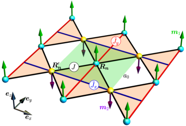
Figure 1: Representation of the Heisenberg checkerboard Hamiltonian in Eq.(1) which consists of two antiferromagnetically coupled square sublattices of magnetic moments $\mu_{s}\bm{m}_{1}(\bm{R}_{\bm{n}})$ and $\mu_{s}\bm{m}_{2}(\bm{R}^{\prime}_{\bm{n}})$ with $\bm{m}_{1,2}$ unit vectors. In addition to the AFM Heisenberg exchange of strength $J$ acting between the nearest neighbors (black bonds), extra Heisenberg interactions of strength $\tilde{J}_{x}$ (blue bonds) and $\tilde{J}_{y}$ (red bonds) act along the corresponding diagonals within the sublattices $\bm{m}_{2}$ and $\bm{m}_{1}$, respectively. We consider the range of parameters corresponding to the compensated AFM ground state with the antiparallel magnetization of the sublattices. The primitive unit cell of the considered two-sublattice system is shown by the green square with side $a_{0}$.

II Heisenberg checkerboard altermagnet

We start from the AM Heisenberg checkerboard Hamiltonian [11] as illustrated in Fig. 1. We consider two square sublattices of discrete classical magnetic moments $\bm{\mu}_{1}(\bm{R}_{\bm{n}})$ and $\bm{\mu}_{2}(\bm{R}^{\prime}_{\bm{n}})$ of fixed magnitude located in the positions determined by the Bravais vectors of each of the sublattices, namely $\bm{R}_{\bm{n}}=a_{0}(n_{x}\bm{e}_{x}+n_{y}\bm{e}_{y})$ and $\bm{R}^{\prime}_{\bm{n}}=\bm{R}_{\bm{n}}-\frac{a_{0}}{2}(\bm{e}_{x}+\bm{e}_{y})$ with $\bm{n}=\{n_{x},n_{y}\}\in\mathbb{Z}\times\mathbb{Z}$, see Fig. 1. Here $a_{0}$ denotes size of the square primitive unit cell of the two-sublattice system. We assume that all magnetic moments have equal amplitude $\mu_{s}$, and therefore, it is instructive to introduce the dimensionless unit vectors $\bm{m}_{1,2}=\bm{\mu}_{1,2}/\mu_{s}$ showing the magnetic moments orientation.

The dynamics of the system under consideration is governed by the set of coupled Landau-Lifshitz equations $\partial_{t}\bm{m}_{1,2}=\frac{\gamma}{\mu_{s}}\left[\bm{m}_{1,2}\times\partial\mathcal{H}/\partial\bm{m}_{1,2}\right]$ where $\gamma>0$ is gyromagnetic ratio, number of equations is equal to the number of magnetic moments, and the coupling is provided by the Hamiltonian

$$\mathcal{H}=J\sum\limits_{\langle\bm{R}_{\bm{n}},\bm{R}^{\prime}_{\bm{n}}\rangle}\bm{m}_{1}(\bm{R}_{\bm{n}})\cdot\bm{m}_{2}(\bm{R}^{\prime}_{\bm{n}})$$ (1)

$$+\sum\limits_{\bm{R}_{\bm{n}}}\Bigl{[}\tilde{J}_{y}\bm{m}_{1}(\bm{R}_{\bm{n}})\cdot\bm{m}_{1}(\bm{R}_{\bm{n}}+a_{0}\bm{e}_{y})-Km_{1z}^{2}-B\mu_{s}m_{1z}\Bigr{]}$$

$$+\sum\limits_{\bm{R}^{\prime}_{\bm{n}}}\Bigl{[}\tilde{J}_{x}\bm{m}_{2}(\bm{R}^{\prime}_{\bm{n}})\cdot\bm{m}_{2}(\bm{R}^{\prime}_{\bm{n}}+a_{0}\bm{e}_{x})-Km_{2z}^{2}-B\mu_{s}m_{2z}\Bigr{]}.$$

Here $J>0$, and, in the first sum, $\bm{R}^{\prime}_{\bm{n}}$ counts the nearest neighbors of $\bm{R}_{\bm{n}}$. Amplitudes of the diagonal interactions $|\tilde{J}_{x,y}|<J$ can generally be different, in this way we take into account the deviation from the altermagnetic limit caused by applied mechanical stress. Additionally, we take into account perpendicular easy-axial anisotropy ($K>0$) and interaction with the magnetic field $\bm{B}=B\bm{e}_{z}$. Here $m_{1z}=\bm{m}_{1}(\bm{R}_{\bm{n}})\cdot\bm{e}_{z}$ and $m_{2z}=\bm{m}_{2}(\bm{R}^{\prime}_{\bm{n}})\cdot\bm{e}_{z}$ with $\bm{e}_{z}=\bm{e}_{x}\times\bm{e}_{y}$.

Assuming that in the ground state magnetic moments are collinear to $\bm{e}_{z}$, we linearize the Landau-Lifshitz equations with respect to the perpendicular components $m_{1,x}$, $m_{1,y}$, $m_{2,x}$, and $m_{2,y}$ and obtain the following dispersion relation for the linear excitations (magnons)

$$\begin{split}&\omega_{\nu}(\bm{k})=\omega_{0}\left(F_{\bm{k}}\pm\Omega_{\bm{k}}^{-}\right)\pm\gamma B,\\ &F_{\bm{k}}=\sqrt{\left(1+\frac{\kappa}{2}-\Omega_{\bm{k}}^{+}\right)^{2}-\cos^{2}\frac{k_{x}a_{0}}{2}\cos^{2}\frac{k_{y}a_{0}}{2}},\\ &\Omega_{\bm{k}}^{\pm}=\frac{\epsilon_{x}\sin^{2}\frac{k_{x}a_{0}}{2}\pm\epsilon_{y}\sin^{2}\frac{k_{y}a_{0}}{2}}{2},\end{split}$$ (2)

for details see Appendix A. Here index $\nu$ numerates two branches corresponding to the signs ‘$+$’ and ‘$-$’ in the right hand side. Frequency $\omega_{0}=4J\gamma/\mu_{s}$ determines the typical time scale of the system. $\kappa=K/J$ is the normalized anisotropy, and $\epsilon_{\alpha}=\tilde{J}_{\alpha}/J$ with $\alpha=x,y$. In the particular case $\kappa=0$ and $B=0$, dispersion (2) reproduces the previously obtained result [12].

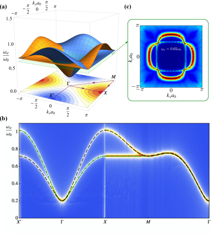
Figure 2: (a) – Dispersion relation (2) within the 1st Brillouin zone for the case $\epsilon_{x}=\epsilon_{y}=0.3$, $\kappa=0.04$, and $B=0$. The value of the splitting between branches is shown by the color code at the bottom. (b) – the comparison of the dispersion (2) with the magnon dispersion obtained using the numerical simulations, for detail see Appendix D. (c) – 2D “surfaces” of constant energy $\omega_{\nu}=0.65\omega_{0}$,

An example of the dispersion relation (2) is shown in Fig. 2, which demonstrates the anisotropic (in $k$-space) splitting of the magnon branches typical for the d-wave altermagnets [3], which for the checkerboard AM are rotated with respect to each other by $\pi/2$. Note the very good agreement with the spectra obtained by means of the numerical simulations, for details see Fig. 2(b) and Appendix D.

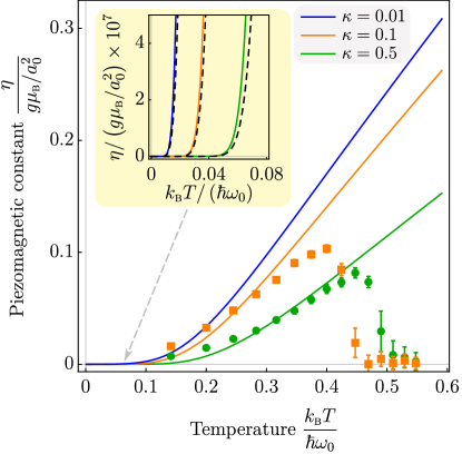
Figure 3: The fluctuation induced piezomagnetic coupling constant $\eta$ as a function of temperature is shown for $\epsilon_{x}=-\epsilon_{y}=0.1$ and for three different anisotropy values. The inset demonstrates the asymptotic behavior (5) (dashed lines) in the limit of low temperature. Symbols correspond to the results of numerical simulations.

II.1 Fluctuation induced piezomagnetism

We now introduce the magnetic moment as a thermodynamic quantity $M=-\partial_{B}F$ [13, 14], where $F$ is the Helmholtz free energy and $B$ is the applied magnetic field . For low enough temperature, magnons can be considered as gas on noninteracting bosons, in this case [16, 17] $F=E_{0}+\frac{1}{\beta}\sum_{\bm{k},\nu}\ln\left(1-e^{-\beta E_{\bm{k},\nu}}\right)$, where $E_{0}$ is energy of the ground state, $\beta=1/(k_{\textsc{b}}T)$ is inverse temperature and $E_{\bm{k},\nu}=\hbar\omega_{\nu}(\bm{k})$ is energy of a magnon. The summation is performed over $\bm{k}$-vectors within the 1st Brillouin zone. Taking into account that the energy $E_{0}$ of the considered ground state does not depend on the applied field, we differentiate the free energy and present the magnetic moment in form

$$M=\sum\limits_{\bm{k},\nu}\frac{\mu_{\bm{k},\nu}}{e^{\beta E_{\bm{k},\nu}}-1},$$ (3)

which enables one to recognize the quantity $\mu_{\bm{k},\nu}=-\partial_{B}E_{\bm{k},\nu}$ as magnetic moment of one magnon [13]. Note that according to (2), one has $\mu_{\bm{k},\nu}=\mp\gamma\hbar=\mp g\mu_{\textsc{b}}$ with $g$ being the $g$-factor and $\mu_{\textsc{b}}>0$ being the Bohr magneton. Thus, the magnons belonging to different branches carry magnetic moments of opposite signs. With the use of (2) and (3) we derive the following expression for the magnetic moment density in vanishing applied magnetic field

$$\mathcal{M}=\frac{g\mu_{\textsc{b}}}{a_{0}^{2}}\!\!\iint\limits_{-\pi}^{\;\;\;\;\;\pi}\!\!\frac{\mathrm{d}q_{x}\mathrm{d}q_{y}}{(2\pi)^{2}}\frac{\sinh\left(\beta^{\prime}\Omega_{\bm{q}}^{-}\right)}{\cosh\left(\beta^{\prime}F_{\bm{q}}\right)-\cosh\left(\beta^{\prime}\Omega_{\bm{q}}^{-}\right)},$$ (4)

where we introduced the magnetization $\mathcal{M}=M/(L_{x}L_{y})$ with $L_{x}L_{y}$ being the altermagnet area, $\bm{q}=a_{0}\bm{k}$ is the dimensionless wave-vector, $\beta^{\prime}=\hbar\omega_{0}/(k_{\textsc{b}}T)$, and we proceed from the summation to integration over the 1st Brillouin zone, assuming the large size of the magnet. Using (2), one can easily show that $\mathcal{M}\to-\mathcal{M}$ under the interchange $\epsilon_{x}\leftrightarrow\epsilon_{y}$. As a consequence, one has $\mathcal{M}=0$ for $\epsilon_{x}=\epsilon_{y}$, i.e. the magnetization vanishes in the AM limit. This property motivates us to write $\mathcal{M}=\eta(\epsilon_{x}-\epsilon_{y})$ introducing the piezomagnetic coupling constant $\eta$. In the limit of low temperatures ($\beta^{\prime}\gg 1$), we estimate integral (4) by means of the Laplace method [18] and obtain

$$\eta\approx\frac{g\mu_{\textsc{b}}}{a_{0}^{2}}f(\epsilon_{x},\epsilon_{y})\frac{\Delta^{2}}{\beta^{\prime}}\ln\frac{1}{1-e^{-\beta^{\prime}\Delta}},$$ (5)

where $\Delta=\sqrt{\kappa(1+\frac{\kappa}{4})}$ is the gap size in units $\hbar\omega_{0}$. For $\epsilon_{\alpha}\ll 1$, function $f$ can be approximated as follows $f\approx\frac{2}{\pi}\left[1-\frac{3}{2}(\epsilon_{x}+\epsilon_{y})\left(1+\frac{\kappa}{2}\right)\right]$, for details see Appendix B.

The temperature evolution of $\eta$ is shown in Fig. 3. For the limit $T\to 0$, it is exponentially suppressed, which is a typical behavior for a gapped system. Anisotropy strengthens the magnetization stiffness of the sublattices, suppressing thermal occupation of magnons and thus the emergent magnetic moment. This is more clearly shown in the inset of Fig. 3. For the special gapless case ($\kappa=0$), the piezomagnetic coupling constant has $T^{3}$-dependence in the limit of small temperatures for this 2D system, namely $\eta\approx\frac{g\mu_{\textsc{b}}}{a_{0}^{2}}\frac{6}{\pi}\zeta(3)/\beta^{\prime 3}$ with $\zeta(x)$ being Riemann zeta-function.

II.2 Fluctuation induced thermal spin conductivity

Let us now consider the possibility of the generation of spin current $j$ by the applied temperature gradient $\bm{\nabla}T$:

$$j_{\alpha}=\sigma_{\alpha\beta}\partial_{\beta}T,$$ (6)

where $\sigma_{\alpha\beta}$ is tensor of thermal spin conductivity. Within the relaxation time approximation [19] we obtain

$$\sigma_{\alpha\beta}=\frac{\tau_{\text{rlx}}}{L_{x}L_{y}}\sum\limits_{\bm{k},\nu}c_{\bm{k},\nu}\left(v_{\bm{k},\nu}\right)_{\alpha}\left(v_{\bm{k},\nu}\right)_{\beta},$$ (7)

where $\tau_{\text{rlx}}$ is the relaxation time – the average time between magnons collisions, $\left(v_{\bm{k},\nu}\right)_{\alpha}=\partial\omega_{\nu}(\bm{k})/\partial k_{\alpha}$ is group velocity, and

$$c_{\bm{k},\nu}=\partial_{T}\frac{\mu_{\bm{k},\nu}}{e^{\beta E_{\bm{k},\nu}}-1}$$ (8)

is spin capacity per magnon. Based on definition (7) and dispersion relation (2) one can show that $\sigma_{xy}=0$. For the case $\epsilon_{x}=\epsilon_{y}$, the additional symmetry $\sigma_{xx}=-\sigma_{yy}$ takes place and the conductivity tensor obtains the following form

$$[\sigma_{\alpha\beta}]=\sigma\begin{bmatrix}-1&0\\ 0&1\end{bmatrix}.$$ (9)

The temperature dependence of the conductivity amplitude $\sigma$ is shown in Fig. 4. According to (9), spin current $\bm{j}$ flows at angle $\pi-\varphi$ to the direction $\bm{e}_{x}$ where $\varphi=\angle(\bm{\nabla}T,\bm{e}_{x})$.

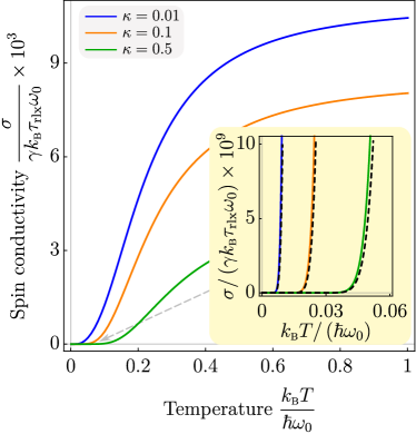
Figure 4: Diagonal elements of the spin conductivity tensor (7) computed for $\epsilon_{x}=\epsilon_{y}=0.1$ and for three different anisotropy values. The inset demonstrates the asymptotic behavior (10) (dashed lines) in the limit of low temperature.

For the case of low temperature $k_{\textsc{b}}T\ll\hbar\omega_{0}$ we obtain $-\sigma_{xx}\approx\sigma_{yy}\approx\sigma$ with

$$\sigma\approx\gamma k_{\textsc{b}}\frac{\omega_{0}\tau_{\text{rlx}}}{2\pi}\Delta^{2}(\epsilon_{x}+\epsilon_{y})\ln\frac{1}{1-e^{-\beta^{\prime}\Delta}}.$$ (10)

For the exact expressions for the components of $\sigma_{\alpha\beta}$, see Appendix C.

III Conclusions

We analyzed the contribution of magnons to the thermodynamic properties an altermagnetic film whose magnetic subsystem is approximated by the checkerboard model. This AM has two important features: (i) it results in the anisotropic (in $k$-space) splitting of the magnon spectra typical for $d$-wave altermagnets, and (ii) it allows an easy relation between the magnetic properties and the applied strain $\propto(\tilde{J}_{x}-\tilde{J}_{y})$. The Landau theory for altermagnets implies a trilinear coupling between strain, ferromagnetic magnetization and the Néel order parameter. Therefore an applied strain leads in general to a ferrimagnetic state: a strain that breaks the AM symmetry allows the magnitude of the moments on the two sublattices to become different (see Appendix E and Ref. [9]). Due to the trilinear coupling this longitudinal response is present in the ground state and vanishes together with the Néel parameter when temperature increases.

Here we have identified a piezomagnetic response that instead grows with temperature, because it is driven by thermally excited magnons and is described by formula (4). This piezomagnetic response is due to transversal magnetic fluctuations and can thus also be expected for systems with fixed local moments. It reaches a maximum in a temperature region just below $T_{\textsc{n}}$. Interestingly, the thermally-induced piezomagnetism is dominant for materials with small magnetic moments $\mu_{s}\ll\mu_{\textsc{b}}$ in the temperature regime $T\lesssim T_{\textsc{n}}$. We have also shown that in presence of magnetic fluctuations a spin current is generated by an applied temperature gradient due to different magnon branches carrying opposite magnetic moment. The spin carried by the heat current couples to the direction of that current. These results are easily generalized to higher dimensions and different lattice geometries.

This fluctuation induced piezomagnetic effect may be of interest for the control of AM domains, which is key for development of AM-based spintronics because macroscopic altermagnetic properties and responses vanish when domains are averaged over. As AM domains are related by time-reversal symmetry [10, 11], their piezomagnetic response has an opposite sign. Thus an energy difference between domains can be induced by applying simultaneously strain and magnetic field in the appropriate directions. Particularly, applying these two during cooling across $T_{\textsc{n}}$ opens an efficient route to favor only one of the domains. As we have shown here precisely in this temperature regime magnetic fluctuations strongly affect the piezomagnetic response.

Appendix A Dispersion relation for the Heisenberg checkerboard model

We start from the linearization of the Landau-Lifshitz equations $\partial_{t}\bm{m}_{1,2}=\frac{\gamma}{\mu_{s}}\left[\bm{m}_{1,2}\times\partial\mathcal{H}/\partial\bm{m}_{1,2}\right]$ with respect to the perpendicular components $m_{1,2;x,y}$ on the top of the ground state $\bm{m}_{1}^{0}=\bm{e}_{z}$, $\bm{m}_{2}^{0}=-\bm{e}_{z}$:

$$\begin{split}&\partial_{t}m_{1\alpha}(\bm{R}_{\bm{n}})=-\varepsilon_{\alpha\beta}\frac{\gamma}{\mu_{s}}\frac{\partial\mathcal{H}^{(2)}}{\partial m_{1\beta}(\bm{R}_{\bm{n}})},\\ &\partial_{t}m_{2\alpha}(\bm{R}^{\prime}_{\bm{n}})=\varepsilon_{\alpha\beta}\frac{\gamma}{\mu_{s}}\frac{\partial\mathcal{H}^{(2)}}{\partial m_{2\beta}(\bm{R}^{\prime}_{\bm{n}})},\end{split}$$ (11)

where $\alpha=x,y$, and the harmonic part of Hamiltonian (1) is as follows

$$\mathcal{H}^{(2)}=\sum\limits_{\alpha=x,y}\biggl{\{} J\!\!\!\sum\limits_{\langle\bm{R}_{\bm{n}},\bm{R}^{\prime}_{\bm{n}}\rangle}m_{1\alpha}(\bm{R}_{\bm{n}})m_{2\alpha}(\bm{R}^{\prime}_{\bm{n}})+\sum\limits_{\bm{R}_{\bm{n}}}\Bigl{[}\tilde{J}_{y}m_{1\alpha}(\bm{R}_{\bm{n}})m_{1\alpha}(\bm{R}_{\bm{n}}+a_{0}\bm{e}_{y})+\left(2J-\tilde{J}_{y}+K+\frac{\mu_{s}B}{2}\right)m_{1\alpha}^{2}(\bm{R}_{\bm{n}})\Bigr{]}$$

$$+\sum\limits_{\bm{R}^{\prime}_{\bm{n}}}\Bigl{[}\tilde{J}_{x}m_{2\alpha}(\bm{R}^{\prime}_{\bm{n}})m_{2\alpha}(\bm{R}^{\prime}_{\bm{n}}+a_{0}\bm{e}_{x})+\left(2J-\tilde{J}_{x}+K-\frac{\mu_{s}B}{2}\right)m_{2\alpha}^{2}(\bm{R}^{\prime}_{\bm{n}})\Bigr{]}\biggr{\}}$$ (12)

Next, we utilize the Fourier transforms on the periodic lattice

$$\begin{split}f(\bm{R}_{\bm{n}})=\frac{1}{\sqrt{N}}\sum\limits_{\bm{k}\in 1.\text{BZ}}\hat{f}(\bm{k})e^{i\bm{k}\cdot\bm{R}_{\bm{n}}},\\ \hat{f}(\bm{k})=\frac{1}{\sqrt{N}}\sum\limits_{\bm{R}_{\bm{n}}}f(\bm{R}_{\bm{n}})e^{-i\bm{k}\cdot\bm{R}_{\bm{n}}}\end{split}$$ (13)

supplemented with the completeness relation $\sum_{\bm{R}_{\bm{n}}}e^{i(\bm{k}-\bm{k}^{\prime})\cdot\bm{R}_{\bm{n}}}=N\delta_{\bm{k},\bm{k}^{\prime}}$. Here $N$ is the number of magnetic moments in one sublattice. Applying (13) to (11), we obtain the equations of motion in reciprocal space

$$\begin{split}&\partial_{t}\hat{m}_{1\alpha}(\bm{k})=-\varepsilon_{\alpha\beta}\frac{\gamma}{\mu_{s}}\frac{\partial\mathcal{H}^{(2)}}{\partial\hat{m}_{1\beta}(-\bm{k})},\\ &\partial_{t}\hat{m}_{2\alpha}(\bm{k})=\varepsilon_{\alpha\beta}\frac{\gamma}{\mu_{s}}\frac{\partial\mathcal{H}^{(2)}}{\partial\hat{m}_{2\beta}(-\bm{k})},\end{split}$$ (14)

Note that the Fourier transform for the sublattice $\bm{R}^{\prime}_{\bm{n}}$ coincides with (13) up to the replacement $\bm{R}_{\bm{n}}\to\bm{R}^{\prime}_{\bm{n}}$. In reciprocal space, the harmonic part of he Hamiltonian (12) is as follows

$$\begin{split}&\mathcal{H}^{(2)}=\sum\limits_{\bm{k}\in 1.\text{BZ}}\biggl{[}4J\cos\frac{a_{0}k_{x}}{2}\cos\frac{a_{0}k_{y}}{2}\hat{m}_{1\alpha}(\bm{k})\hat{m}_{2\alpha}(-\bm{k})\\ &+\left(2J-2\tilde{J}_{y}\sin^{2}\frac{k_{y}a_{0}}{2}+K+\frac{\mu_{s}B}{2}\right)\hat{m}_{1\alpha}(\bm{k})\hat{m}_{1\alpha}(-\bm{k})\\ &+\left(2J-2\tilde{J}_{x}\sin^{2}\frac{k_{x}a_{0}}{2}+K-\frac{\mu_{s}B}{2}\right)\hat{m}_{2\alpha}(\bm{k})\hat{m}_{2\alpha}(-\bm{k})\biggr{]},\end{split}$$ (15)

where the summation over the repeating index $\alpha\in\{x,y\}$ is assumed. With (15), we write Eqs. (14) in the form

$$\partial_{t}\bm{\xi}=\omega_{0}\mathbb{M}\bm{\xi},$$ (16)

where $\bm{\xi}=(\hat{m}_{1x},\hat{m}_{1y},\hat{m}_{2x},\hat{m}_{2y})^{\textsc{t}}$, and matrix $\mathbb{M}$ is as follows

$$\mathbb{M}=\begin{bmatrix}0&-(\mathcal{B}_{y}+b)&0&-\mathcal{A}\\ \mathcal{B}_{y}+b&0&\mathcal{A}&0\\ 0&\mathcal{A}&0&\mathcal{B}_{x}-b\\ -\mathcal{A}&0&-(\mathcal{B}_{x}-b)&0\end{bmatrix}$$ (17a)

with $$b=\mu_{s}B/(4J)$$ and

$$\mathcal{A}=\cos\frac{k_{x}a_{0}}{2}\cos\frac{k_{x}a_{0}}{2},$$ (17b)

$$\mathcal{B}_{\alpha}=1+\frac{\kappa}{2}-\epsilon_{\alpha}\sin^{2}\frac{k_{\alpha}a_{0}}{2}.$$ (17c)

Parameters $\omega_{0}$, $\kappa$, and $\epsilon_{\alpha}$ are defined in the main text. System (16) has solution $\bm{\xi}=\bm{\xi}_{0}e^{-i\omega t}$, which is nontrivial ($\bm{\xi}_{0}\neq\bm{0}$) if $\omega=i\omega_{0}\lambda_{\nu}$ with $\lambda_{\nu}$ being the eigenvalues of matrix $\mathbb{M}$. The eigenvalues $\lambda_{\nu}$ are imaginary and compose two complex-conjugated pairs. The pair of the non-negative eigenfrequencies is presented in (2). Note that $\gamma B=\omega_{0}b$.

Appendix B Magnetization for low temperature

The explicit form of function $f(\epsilon_{x},\epsilon_{y})$ is as follows

$$\begin{split}&f=\frac{2}{\pi^{2}\delta\epsilon}\int\limits_{0}^{\pi}\biggl{\{}\left[1+\left(1+\frac{\kappa}{2}\right)(\bar{\epsilon}+\delta\epsilon\cos\chi)\right]^{2}\\ &-\Delta^{2}(\delta\epsilon+\bar{\epsilon}\cos\chi)^{2}\biggr{\}}^{-1}(\delta\epsilon+\bar{\epsilon}\cos\chi)\,\mathrm{d}\chi,\end{split}$$ (18)

where we introduced $\delta\epsilon=(\epsilon_{x}-\epsilon_{y})/2$ and $\bar{\epsilon}=(\epsilon_{x}+\epsilon_{y})/2$. In the limit $\delta\epsilon\ll 1$, we obtain

$$f=\frac{2/\pi}{\left\{\left[1+(1+\frac{\kappa}{2})\bar{\epsilon}\right]^{2}-\Delta^{2}\bar{\epsilon}^{2}\right\}^{3/2}}+\mathcal{O}(\delta\epsilon^{2}).$$ (19)

Assuming $\bar{\epsilon}\ll 1$, one obtains the approximation presented in the main text.

Appendix C Tensor of thermal spin conductivity

The exact expressions for $\sigma_{\alpha\beta}$ defined in (7) are as follows

$$\begin{split}&\sigma_{xx}=-\gamma k_{\textsc{b}}\beta^{\prime 2}\frac{\tau_{\text{rlx}}\omega_{0}}{64}\iint\limits_{-\pi}^{\pi}\frac{\mathrm{d}q_{x}\mathrm{d}q_{y}}{(2\pi)^{2}}\sin^{2}q_{x}\\ &\times\Biggl{\{}\frac{(F_{q}+\Omega_{q}^{-})\left[\frac{1}{F_{q}}\left(\cos^{2}\frac{q_{y}}{2}-\epsilon_{x}\left(1+\frac{\kappa}{2}-\Omega_{q}^{+}\right)\right)+\epsilon_{x}\right]^{2}}{\sinh^{2}\left[\frac{\beta^{\prime}}{2}(F_{q}+\Omega_{q}^{-})\right]}\\ &-\frac{(F_{q}-\Omega_{q}^{-})\left[\frac{1}{F_{q}}\left(\cos^{2}\frac{q_{y}}{2}-\epsilon_{x}\left(1+\frac{\kappa}{2}-\Omega_{q}^{+}\right)\right)-\epsilon_{x}\right]^{2}}{\sinh^{2}\left[\frac{\beta^{\prime}}{2}(F_{q}-\Omega_{q}^{-})\right]}\Biggr{\}}\end{split}$$ (20)

and

$$\begin{split}&\sigma_{yy}=-\gamma k_{\textsc{b}}\beta^{\prime 2}\frac{\tau_{\text{rlx}}\omega_{0}}{64}\iint\limits_{-\pi}^{\pi}\frac{\mathrm{d}q_{x}\mathrm{d}q_{y}}{(2\pi)^{2}}\sin^{2}q_{y}\\ &\times\Biggl{\{}\frac{(F_{q}+\Omega_{q}^{-})\left[\frac{1}{F_{q}}\left(\cos^{2}\frac{q_{x}}{2}-\epsilon_{y}\left(1+\frac{\kappa}{2}-\Omega_{q}^{+}\right)\right)-\epsilon_{y}\right]^{2}}{\sinh^{2}\left[\frac{\beta^{\prime}}{2}(F_{q}+\Omega_{q}^{-})\right]}\\ &-\frac{(F_{q}-\Omega_{q}^{-})\left[\frac{1}{F_{q}}\left(\cos^{2}\frac{q_{x}}{2}-\epsilon_{y}\left(1+\frac{\kappa}{2}-\Omega_{q}^{+}\right)\right)+\epsilon_{y}\right]^{2}}{\sinh^{2}\left[\frac{\beta^{\prime}}{2}(F_{q}-\Omega_{q}^{-})\right]}\Biggr{\}}\end{split}$$ (21)

and $\sigma_{xy}=\sigma_{yx}=0$.

Appendix D Numerical simulations of the Heisenberg checkerboard

We consider a square lattice with lattice constant $a_{0}$. Each node is characterized by a magnetic moment $\bm{m}_{i}$, and index $i$ defines the position of magnetic moment on the lattice with size $N_{1}\times N_{2}$. The dynamics of the magnetic system is governed by the stochastic Landau–Lifshitz equations

$$\begin{split}\frac{\mathrm{d}\bm{m}_{i}}{\mathrm{d}t}&=-\frac{\gamma}{1+\alpha^{2}}\left[1+\alpha\,\bm{m}_{i}\times\right]\bm{m}_{i}\times\bm{H}_{i}^{\textsc{eff}},\\ \bm{H}_{i}^{\textsc{eff}}&=-\frac{1}{\mu_{s}}\frac{\partial\mathcal{H}}{\partial\bm{m}_{i}}+\bm{H}_{i}^{\textsc{th}},\end{split}$$ (22)

where $\alpha$ is a Gilbert damping parameter, $\mathcal{H}$ is defined in (1), and $\bm{H}_{i}^{\textsc{th}}$ is a stochastic thermal field given by

$$\bm{H}_{i}^{\textsc{th}}\left(t\right)=\sqrt{2\mathcal{D}}\bm{\zeta}_{i}\left(t\right)=\sqrt{2\frac{\alpha\,k_{\textsc{b}}T}{\gamma\mu_{s}}}\bm{\zeta}_{i}\left(t\right),$$ (23)

where the magnitude is given by the fluctuation-dissipation theorem and $\bm{\zeta}_{i}$ is white noise, such that the ensemble average and variance of the thermal field fulfill $\left<\bm{H}_{i\alpha}^{\textsc{th}}(t)\right>=0$ and $\left<\bm{H}_{i\alpha}^{\textsc{th}}(0)\bm{H}_{j\beta}^{\textsc{th}}(t)\right>=2\mathcal{D}\delta_{ij}\delta_{\alpha\beta}\delta(t)$, respectively. To achieve these properties in an implementation, the vectors $\bm{\zeta}_{i}$ can each be created from three independent standard normally distributed random values at every time step. Note also that in time-integration schemes, to fulfill the fluctuation-dissipation relation, the thermal field needs to be normalized by the time step with a factor $1/\sqrt{\delta t}$.

To evolve a magnetic system in time according to equation (22) we used Heun’s method for temperature-induced effects [20, 21, 22], and a fourth-order Runge-Kutta method in other cases. During the integration process, the condition $\left|\bm{m}_{i}(t)\right|=1$ is controlled.

D.1 Simulation of spinwaves

To simulate spinwaves we considered a system with a size of $N_{1}\times N_{2}=500\times 500$ magnetic moments. The simulations are carried out in two steps. In the first step, we simulate the dynamics of the system in the external magnetic field $\bm{B}_{i}=B_{0}\,\text{sinc}\left(2\pi\ \bm{k}\cdot\bm{R}_{i}\right)\text{sinc}\left[2\pi\omega_{0}\left(t-t_{0}\right)\right]$, where $t_{0}=t_{\text{sim}}/2$ is a center of temporal part of field profile and $H_{0}$ is an amplitude of the applied field. The simulations are performed in the low damping regime with $\alpha=10^{-3}$.

In the second step we performed a space-time transform for the complex-valued parameter $m_{i}^{\textsc{x}}(t)+i\ m_{i}^{\textsc{y}}(t)$. The resulting eigenfrequencies are plotted in Fig. 2.

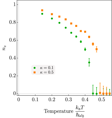
Figure 5: Temperature dependence of perpendicular component of Néel vector $n_{z}$ is shown for $\epsilon_{x}=-\epsilon_{y}=0.1$ and for two different anisotropy values. Symbols correspond to the results of numerical simulations.

D.2 Simulation of temperature-induced effects

Here we consider a system with a size of $N_{1}\times N_{2}=1000\times 1000$ magnetic moments. In the simulations, we consider the temperature in the range $T\in\left[0.15;\,0.55\right]\hbar\omega_{0}/k_{\textsc{b}}$. The simulations were performed for a low damping regime with $\alpha=10^{-3}$ for a long time scale with $\alpha t\omega_{0}\gg 1$. The averaged perpendicular net magnetization and Néel vectors are presented in Figs. 3 and 5, respectively. Note that the averaged in-plane components of the net magnetization vanish.

Appendix E Continuous model and the strain-induced ferrimagnetism

In the discrete Hamiltonian (1), we perform the Taylor expansion $\bm{m}_{\nu}(\bm{R}_{\bm{n}}+\delta\bm{R})\approx\bm{m}_{\nu}(\bm{R}_{\bm{n}})+(\delta\bm{R})_{\alpha}\partial_{\alpha}\bm{m}_{\nu}+\frac{1}{2}(\delta\bm{R})_{\alpha}(\delta\bm{R})_{\beta}\partial_{\alpha\beta}^{2}\bm{m}_{\nu}$ and proceed from the summation to integration in the way $\sum_{\bm{R}_{\bm{n}}}(\dots)\to a_{0}^{-2}\int(\dots)\mathrm{d}x\mathrm{d}y$. The continuous approximation of (1) obtained in this way is $\mathcal{H}=\int\mathscr{H}\mathrm{d}x\mathrm{d}y$ with density

$$\begin{split}&\mathscr{H}=\frac{1}{a_{0}^{2}}\left[4J\,\bm{m}_{1}\cdot\bm{m}_{2}+\tilde{J}_{y}|\bm{m}_{1}|^{2}+\tilde{J}_{x}|\bm{m}_{2}|^{2}\right]\\ &-J\,\partial_{\alpha}\bm{m}_{1}\cdot\partial_{\alpha}\bm{m}_{2}-\frac{\tilde{J}_{y}}{2}|\partial_{y}\bm{m}_{1}|^{2}-\frac{\tilde{J}_{x}}{2}|\partial_{x}\bm{m}_{2}|^{2}\\ &-\frac{1}{a_{0}^{2}}\sum\limits_{\nu=1,2}(Km_{\nu z}^{2}+B\mu_{s}m_{\nu z}).\end{split}$$ (24)

In terms of the Néel $\bm{\mathrm{n}}=\frac{1}{2}(\bm{m}_{1}-\bm{m}_{2})$ and magnetization $\bm{\mathrm{m}}=\frac{1}{2}(\bm{m}_{1}+\bm{m}_{2})$ vectors, we present (24) in form

$$\begin{split}\mathscr{H}\approx&\mathscr{H}_{\text{hom}}+\mathcal{A}_{\alpha\beta}\partial_{\alpha}\bm{\mathrm{n}}\cdot\partial_{\beta}\bm{\mathrm{n}}+\tilde{\mathcal{A}}_{\alpha\beta}\partial_{\alpha}\bm{\mathrm{n}}\cdot\partial_{\beta}\bm{\mathrm{m}}\\ &-\frac{2}{a_{0}^{2}}(K\mathrm{n}_{z}^{2}+B\mu_{s}\mathrm{m}_{z}).\end{split}$$ (25)

Here $[\mathcal{A}_{\alpha\beta}]=\text{diag}(J-\frac{1}{2}\tilde{J}_{x},J-\frac{1}{2}\tilde{J}_{y})$, and $[\tilde{\mathcal{A}}_{\alpha\beta}]=\text{diag}(\tilde{J}_{x},-\tilde{J}_{y})$, and we neglected quadratic in $m$ terms except the homogeneous exchange contribution

$$\begin{split}\mathscr{H}_{\text{hom}}=\frac{1}{a_{0}^{2}}\biggl{[}&-a_{\textsc{gl}}|\bm{\mathrm{n}}|^{2}+\frac{b_{\textsc{gl}}}{2}|\bm{\mathrm{n}}|^{4}\\ &+4J|\bm{\mathrm{m}}|^{2}-2(\tilde{J}_{x}-\tilde{J}_{y})\bm{\mathrm{n}}\cdot\bm{\mathrm{m}}\biggr{]}.\end{split}$$ (26)

Here $a_{\textsc{gl}}=4J-\tilde{J}_{x}-\tilde{J}_{y}>0$ and additionally we introduce the nonlinear Ginzburg-Landau term with $b_{\textsc{gl}}>0$ which stabilizes the length of the Néel order parameter. Note that $|\bm{m}_{1}|\neq|\bm{m}_{2}|$ if $\tilde{J}_{x}\neq\tilde{J}_{y}$, and therefore $\bm{\mathrm{n}}\cdot\bm{\mathrm{m}}\neq 0$ in general case. In the leading order in $\tilde{J}_{\alpha}$ the minimization of $\mathscr{H}_{\text{hom}}$ with respect to $\bm{\mathrm{n}}$ and $\bm{\mathrm{m}}$ results in

$$\bm{\mathrm{m}}=\frac{\epsilon_{x}-\epsilon_{y}}{4}\bm{\mathrm{n}},\qquad|\bm{\mathrm{n}}|\approx\sqrt{\frac{a_{\textsc{gl}}}{b_{\textsc{gl}}}},$$ (27)

where $\epsilon_{\alpha}=\tilde{J}_{\alpha}/J$. The corresponding magnetic moment density is $\mathcal{M}=\eta_{\textsc{fm}}(\epsilon_{x}-\epsilon_{y})$ where $\eta_{\textsc{fm}}=\mu_{s}|\bm{\mathrm{n}}|/(2a_{0}^{2})$ is the piezomagnetic coupling constant which originates from the strain-induced ferrimagnetism. In contrast to $\eta_{\textsc{fm}}$, the fluctuations related piezomagnetic constant $\eta$ does not depend on $\mu_{s}$, see Fig. 3. This is a consequence of the fact that magnetic moment of a magnon $\pm\gamma\hbar$ does not depend on $\mu_{s}$. As a result, for materials with $\mu_{s}\ll\mu_{\textsc{b}}$, we expect that $\eta\gg\eta_{\textsc{fm}}$ in the limit of high temperatures $T\lesssim T_{\textsc{n}}$. In this temperature regime, $\eta$ has the highest value while $|\bm{\mathrm{n}}|$ decreases leading also to the additional decrease of $\eta_{\textsc{fm}}$.

References

- Šmejkal et al. [2020] L. Šmejkal, R. González-Hernández, T. Jungwirth, and J. Sinova, Crystal time-reversal symmetry breaking and spontaneous hall effect in collinear antiferromagnets, Science Advances 6, eaaz8809 (2020).
- Šmejkal et al. [2022] L. Šmejkal, J. Sinova, and T. Jungwirth, Beyond conventional ferromagnetism and antiferromagnetism: A phase with nonrelativistic spin and crystal rotation symmetry, Phys. Rev. X 12, 031042 (2022).
- Šmejkal et al. [2022] L. Šmejkal, J. Sinova, and T. Jungwirth, Emerging research landscape of altermagnetism, Physical Review X 12, 040501 (2022).
- Naka et al. [2019] M. Naka, S. Hayami, H. Kusunose, Y. Yanagi, Y. Motome, and H. Seo, Spin current generation in organic antiferromagnets, Nature Communications 10, 4305 (2019), arXiv:1902.02506 [cond-mat.str-el] .
- Yuan et al. [2020] L.-D. Yuan, Z. Wang, J.-W. Luo, E. I. Rashba, and A. Zunger, Giant momentum-dependent spin splitting in centrosymmetric low- antiferromagnets, Phys. Rev. B 102, 014422 (2020).
- Naka et al. [2021] M. Naka, Y. Motome, and H. Seo, Perovskite as a spin current generator, Phys. Rev. B 103, 125114 (2021).
- Guo et al. [2023] Y. Guo, H. Liu, O. Janson, I. C. Fulga, J. van den Brink, and J. I. Facio, Spin-split collinear antiferromagnets: A large-scale ab-initio study, Materials Today Physics 32, 100991 (2023).
- Sato et al. [2023] T. Sato, S. Haddad, I. C. Fulga, F. F. Assaad, and J. van den Brink, Altermagnetic anomalous hall effect emerging from electronic correlations (2023), arXiv:2312.16290 [cond-mat.str-el] .
- McClarty and Rau [2023] P. A. McClarty and J. G. Rau, Landau theory of altermagnetism (2023), arXiv:2308.04484 [cond-mat.mtrl-sci] .
- Aoyama and Ohgushi [2024] T. Aoyama and K. Ohgushi, Piezomagnetic properties in altermagnetic mnte, Phys. Rev. Mater. 8, L041402 (2024).
- Gomonay et al. [2024] O. Gomonay, V. P. Kravchuk, R. Jaeschke-Ubiergo, K. V. Yershov, T. Jungwirth, L. Šmejkal, J. van den Brink, and J. Sinova, Structure, control, and dynamics of altermagnetic textures (2024), arXiv:2403.10218 [cond-mat.mes-hall] .
- Canals [2002] B. Canals, From the square lattice to the checkerboard lattice: Spin-wave and large- limit analysis, Physical Review B 65, 10.1103/physrevb.65.184408 (2002).
- Ashcroft and Mermin [1976] N. W. Ashcroft and N. Mermin, Solid State Physics (Cengage Learning, Inc, 1976).
- Aharoni [1996] A. Aharoni, Introduction to the theory of Ferromagnetism (Oxford University Press, 1996).
- Note [1] is the magnetic moment along the applied field .
- Lifshitz and Pitaevsky [1999] E. M. Lifshitz and L. P. Pitaevsky, Statistical physics, part 2: theory of the condensed state (Butterworth–Heinemann, Linacre House, Jordan Hill, Oxford, 1999).
- Akhiezer et al. [1968] A. I. Akhiezer, V. G. Bar’yakhtar, and S. V. Peletminskiĭ, Spin waves, edited by G. Höhler (North–Holland, Amsterdam, 1968).
- Bender and Orszag [1999] C. M. Bender and S. A. Orszag, Advanced Mathematical Methods for Scientists and Engineers I (Springer New York, 1999).
- Kittel [2005] C. Kittel, Introduction to Solid State Physics, 8th ed. (John Wiley & Sons, 2005).
- [20] U. Nowak, Thermally activated reversal in magnetic nanostructures, in Annual Reviews of Computational Physics IX, pp. 105–151.
- Mentink et al. [2010] J. H. Mentink, M. V. Tretyakov, A. Fasolino, M. I. Katsnelson, and T. Rasing, Stable and fast semi-implicit integration of the stochastic landau–lifshitz equation, Journal of Physics: Condensed Matter 22, 176001 (2010).
- Evans et al. [2014] R. F. L. Evans, W. J. Fan, P. Chureemart, T. A. Ostler, M. O. A. Ellis, and R. W. Chantrell, Atomistic spin model simulations of magnetic nanomaterials, Journal of Physics: Condensed Matter 26, 103202 (2014).