Ab initio calculation of hyper-neutron matter

Abstract

The equation of state (EoS) of neutron matter plays a decisive role in our understanding of the properties of neutron stars as well as the generation of gravitational waves in neutron star mergers. At sufficient densities, it is known that the appearance of hyperons generally softens the EoS, thus leading to a reduction in the maximum mass of neutron stars well below the observed values of about 2 solar masses. Even though repulsive three-body forces are known to solve this so-called “hyperon puzzle”, so far performing ab initio calculations with a substantial number of hyperons has remained elusive. In this work, we address this challenge by employing simulations based on Nuclear Lattice Effective Field Theory with up to 232 neutrons (pure neutron matter) and up to 116 $\Lambda$ hyperons (hyper-neutron matter) in a finite volume. We introduce a novel auxiliary field quantum Monte Carlo algorithm, allowing us to simulate for both pure neutron matter and hyper-neutron matter systems up to 5 times the density of nuclear matter using a single auxiliary field without any sign oscillations. Also, for the first time in ab initio calculations, we not only include $N\Lambda$ two-body and $NN\Lambda$ three-body forces, but also $\Lambda\Lambda$ and $N\Lambda\Lambda$ interactions. Consequently, we determine essential astrophysical quantities such as the mass-radius relation, the speed of sound and the tidal deformability of neutron stars. Our findings also confirm the existence of the $I$-Love-$Q$ relation, which gives access to the moment of inertia of the neutron star.

Introduction

In the era of multi-messenger astronomy, neutron stars arguably stand out as the most captivating astrophysical objects Abbott et al. (2017, 2018); Huth et al. (2022). Neutron stars consist of the densest form of baryonic matter observed in the universe, and within their interiors, exotic new forms of matter may exist Lattimer and Prakash (2004); Gal et al. (2016); Burgio et al. (2021). With the detection of various neutron star phenomena in recent years, such as gravitational waves and electromagnetic radiation, more valuable information regarding the mysterious dense matter within their cores will be unraveled. These findings, together with the measurements of the masses or radii, strongly constrain the neutron star matter equation of state (EoS) and theoretical models of their composition. However, the observation of neutron star masses above $2.0M_{\odot}$ has ruled out many predictions of exotic non-nucleonic components. Resolving this problem, known as the hyperon puzzle, is crucial for understanding the complex interplay between strong nuclear forces and the behavior of dense matter under extreme conditions. For more details and discussions of this topic, see Refs. Djapo et al. (2010); Vidana et al. (2011); Schulze and Rijken (2011); Lonardoni et al. (2015); Astashenok et al. (2014); Chatterjee and Vidaña (2016); Maslov et al. (2015); Haidenbauer et al. (2017); Masuda et al. (2016); Logoteta et al. (2019); Gerstung et al. (2020); Friedman and Gal (2023).

In this study, we use the framework of Nuclear Lattice Effective Field Theory (NLEFT) Lee (2009); Lähde and Meißner (2019) to gain new insights into the generation of hyperons, more specifically $\Lambda(1116)$ particles, within dense environments. To enable calculations with arbitrary numbers of nucleons and hyperons using only one auxiliary field, we introduce a novel formulation of the auxiliary field quantum Monte Carlo (AFQMC) algorithm, which allows for more accurate and efficient simulations free of sign oscillations. Additionally, we incorporate two-body $N\Lambda$ and $\Lambda\Lambda$ interactions, as well as three-body terms such as $NN\Lambda$ and $N\Lambda\Lambda$, based on the minimal nuclear interaction model Lu et al. (2019), into the pionless effective field theory for nucleons. Initially, we focus on systems consisting solely of nucleons and determine the low-energy constants parameterizing the $2N$ and the $3N$ forces by constraining them to the saturation properties of symmetric nuclear matter, as it is well-known that fixing the $3N$ forces in light nuclei leads to a serious overbinding in heavier systems Pieper and Wiringa (2001); Hüther et al. (2020) if mostly local forces are employed. Subsequently, we introduce $\Lambda$-particles into our framework and determine the parameters of the $N\Lambda$ and $\Lambda\Lambda$ interactions by fitting them to experimental data, including the $N\Lambda$ cross section Sechi-Zorn et al. (1968); Alexander et al. (1968); Kadyk et al. (1971); Hauptman et al. (1977) and the $\Lambda\Lambda$ ${}^{1}S_{0}$ scattering phase shift from chiral effective field theory Haidenbauer et al. (2016), respectively. The $NN\Lambda$ and $N\Lambda\Lambda$ forces are further constrained by the separation energies of single- and double-$\Lambda$ hypernuclei, spanning systems from ${}_{\Lambda}^{5}$He to ${}_{\Lambda\Lambda}^{10}$Be. After constructing our interactions, we perform predictive calculations for the EoS of pure neutron matter (PNM) by considering up to 232 neutrons in a box to achieve densities up to five times the empirical saturation density of nuclear matter, i.e., $\rho=0.8$ fm^-3. Our results for the EoS of PNM are in very good agreement with ab-initio calculations using chiral interactions up to N3LO Lynn et al. (2016); Drischler et al. (2019); Keller et al. (2023); Elhatisari et al. (2022) within given density range.

In the next step, we perform simulations for hyper-neutron matter by including up to 116 hyperons in the box and calculate the corresponding EoS, which is called hyper-neutron matter (I), short HNM(I). Not surprisingly, we find that this EoS is too soft to support heavy neutron stars. Therefore, similar to using the saturation properties of symmetric nuclear matter to pin down the three-nucleon forces (3NFs), we redefine the $NN\Lambda$ and $N\Lambda\Lambda$ forces by using the maximal neutron star mass as an observable. Setting $M_{\max}/M_{\odot}=1.9$ and $2.1$, respectively, we generate stiffer EoSs, denoted as HNM(II) and HNM(III), in order. More details on the construction of the actions underlying PNM EoS and the three variants of HNM are given in Methods.

Results and discussion

The results for pure neutron matter and hyper-neutron matter are presented from our state-of-art nuclear lattice simulations. HNM is composed of neutrons and $\Lambda$ hyperons, where $\rho_{N}$, $\rho_{\Lambda}$, and $\rho=\rho_{N}+\rho_{\Lambda}$ are the neutron, $\Lambda$ hyperon and total baryon density of the system, respectively, and $x_{\Lambda}=\rho_{\Lambda}/\rho$ is the fraction of $\Lambda$ hyperons. The $\Lambda$ threshold densities $\rho_{\Lambda}^{\rm th}$ is determined by imposing the equilibrium condition $\mu_{N}=\mu_{\Lambda}$, where the chemical potentials for neutrons $\mu_{N}$ and lambdas $\mu_{\Lambda}$ are evaluated via the derivatives of the energy density $\varepsilon_{\scriptscriptstyle\rm HNM}$,

$$\mu_{N}(\rho,x_{\Lambda})=\frac{\partial\varepsilon_{\scriptscriptstyle\rm HNM}}{\partial\rho_{N}},~{}~{}\mu_{\Lambda}(\rho,x_{\Lambda})=\frac{\partial\varepsilon_{\scriptscriptstyle\rm HNM}}{\partial\rho_{\Lambda}},$$ (1)

which indicates that an accurate determination of the chemical potentials necessitates computing the energy density for various densities and different numbers of $\Lambda$ hyperons.

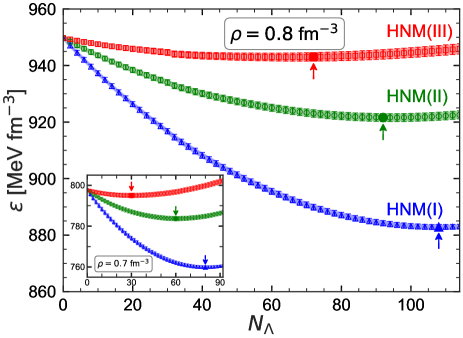
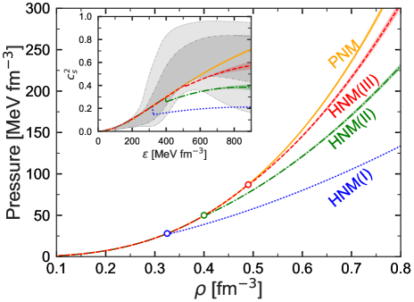
Figure 1: Left Panel: Energy density for hyper-neutron matter (HNM). The energy density $\epsilon$ as a function of different numbers for $\Lambda$ hyperons is shown for densities $\rho=0.8$ fm^-3 and $0.7$ fm^-3 (inset). The blue triangles, green circles, and red squares represent the energy density $\epsilon$ of HNM with hyperons interacting via the two-body interactions and the three-body interactions. The differences between HNM(I), HNM(II) and HNM(III) are the three-body $NN\Lambda$ and $N\Lambda\Lambda$ interactions. The shaded regions represent the uncertainty from the three-baryon forces and Monte Carlo errors. The arrows and the solid triangle, circle, and square denote the lowest energy density. Right Panel: EoS for HNM. The orange solid curve denotes pure neutron matter, obtained from the $NN$ and $NNN$ interactions. The red dashed line represents the EoS of HNM with hyperons interacting via the two-body interactions ($N\Lambda$ and $\Lambda\Lambda$) and the third set of three-body hyperon-nucleon interaction ($NN\Lambda$ and $N\Lambda\Lambda$). The blue dotted curve and the green dot-dashed curve are calculated with the first and second sets of three-body hyperon-nucleon interactions. The $\Lambda$ threshold densities $\rho_{\Lambda}^{\rm th}$ are marked by open circles. In the inset, the speed of sound corresponding to the PNM and HNM EOSs is shown. The gray shaded regions are the inference of the speed of sound for neutron star matter in view of the recent observational data Brandes et al. (2023).

The energy density $\epsilon$ by using the two-body interactions ($NN,N\Lambda,\Lambda\Lambda$) and the three-body interactions ($NNN,NN\Lambda,N\Lambda\Lambda$) are shown in Fig. 1 (left panel) for different numbers of $\Lambda$ hyperons. The differences between HNM(I), HNM(II), and HNM(III) are the three-body $NN\Lambda$ and $N\Lambda\Lambda$ interactions, as detailed in Methods. The shaded regions represent the uncertainty from the three-baryon forces and Monte Carlo errors. The given density of $\rho=0.8$ fm^-3, which is about five times the empirical nuclear matter saturation density, $\rho_{0}$, can be encountered in the core of a neutron star. It should be noted that the quantity of $\Lambda$ hyperons corresponding to the lowest energy density is intricately linked to accurately determining the chemical equilibrium conditions. In contrast to the groundbreaking study Lonardoni et al. (2015) where the number of $\Lambda$ hyperons was varied from 1 to 14, the present study indicates that the number of required $\Lambda$ hyperons is comparable to the number of neutrons, especially at high densities. For instance, as depicted in Fig. 1 (left panel), to fulfill the equilibrium condition $\mu_{N}=\mu_{\Lambda}$ at $\rho=0.8$ fm^-3, 108, 92, and 72 $\Lambda$ hyperons are required to obtain the lowest energy density for HNM(I), HNM(II), and HNM(III), respectively. Similarly, at $\rho=0.7$ fm^-3, 80, 60, and 30 hyperons are needed for the same purpose in HNM(I), HNM(II), and HNM(III), in order.

In Fig. 1 (right panel), the EoSs for PNM and for HNM are displayed. The threshold density is $\rho_{\Lambda}^{\rm th}=0.325(2)(4)$ fm^-3 for HNM(I). Here and what follows, the first/second error is the statistical/systematic one. Several phenomenological schemes Weber and Weigel (1989); Balberg and Gal (1997); Tolos et al. (2017) or microscopical models Baldo et al. (1998); Djapo et al. (2010); Schulze and Rijken (2011) predict that hyperons may appear in the inner core of neutron stars at densities around $\rho\approx(2-3)\rho_{0}$. To explore the impact of the hyperon-nucleon three-body forces on the threshold densities and the stiffness of the EOS at higher densities, the threshold densities for HNM(II) and HNM(III) are 0.400(2)(5) fm^-3 and 0.495(2)(6) fm^-3 by gradually increasing the coupling strength of the three-body hyperon-nucleon interactions. As anticipated, the inclusion of hyperons results in a softer EoS and HNM(III) is the stiffest EoS when hyperons are included. The squared speed of sound, $c_{s}^{2}$, is also shown in the inset of Fig. 1. It is observed that the causality limit ($c_{s}^{2}<1$) is fulfilled for both PNM and HNM. The EoS characterized by nucleonic degrees of freedom exclusively demonstrate a monotonic increase in $c_{s}^{2}$ with increasing energy density. The appearances of $\Lambda$ hyperons, however, induces changes in this behavior, leading to non-monotonic curves that signify the incorporation of additional degrees of freedom. The onset of $\Lambda$ hyperons precipitates a sharp reduction in the speed of sound, marking a significant transition in the stiffness of the EoS. For comparison, the constraints on $c_{s}^{2}$ within the interiors of neutron stars inferred by a Bayesian inference method are also shown Brandes et al. (2023). These constraints are established based on recent multi-messenger data, in combination with limiting conditions from nuclear physics at low densities, as depicted by the gray shaded regions. See Ref. Koehn et al. (2024) for a review and Ref. Essick et al. (2021) for a detailed analysis using employed recent astronomical data. The results for PNM and HNM(III) agree well with the marginal posterior probability distributions at the 95% and 68% levels. Note, however, the neutron stars in general have a small proton fraction, which is neglected in the present work.

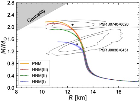
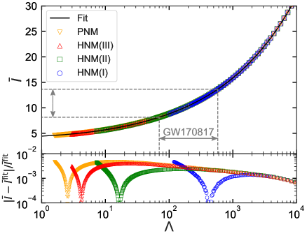
Figure 2: Left Panel: Neutron star mass-radius relation. The legend is the same as of Fig. 1. The gray horizontal dotted line represents 2$M_{\odot}$. The inner and outer contours indicate the allowed area of mass and radius of neutron stars by NICER’s analysis of PSR J0030+0451 Miller et al. (2019) and PSR J0740+6620 Riley et al. (2021). The excluded causality region is also shown by the grey shaded region Lattimer and Prakash (2007). Right Panel: $I$-Love relation. (Top) Universal relations for PNM and HNM together within the slow-rotation approximation with their fitting curves. (Bottom) Absolute fractional difference between the fit curves and the numerical results.

The “holy grail” of neutron-star structure, the mass-radius (MR) relation, is displayed in Fig. 2 (left panel). These relations for PNM and HNM are obtained by solving the Tolman-Oppenheimer-Volkoff (TOV) equations Tolman (1939); Oppenheimer and Volkoff (1939) with the EoSs of Fig. 1. The appearance of $\Lambda$ hyperons in neutron star matter remarkably reduces the predicted maximum mass compared to the PNM scenario. The maximum mass for PNM, HNM(I), HNM(II), and HNM(III) are 2.19(1)(2) $M_{\odot}$, 1.52(1)(1) $M_{\odot}$, 1.93(1)(1) $M_{\odot}$, and 2.12(1)(2) $M_{\odot}$, respectively. Three neutron stars have been measured to have gravitational masses close to $2M_{\odot}$: PSR J1614-2230, with $M=1.908\pm 0.016~{}M_{\odot}$ Demorest et al. (2010); Fonseca et al. (2016); Arzoumanian et al. (2018); PSR J0348+0432, with $2.01\pm 0.04~{}M_{\odot}$ Antoniadis et al. (2013); and PSR J0740+6620, with $2.08\pm 0.07~{}M_{\odot}$ Cromartie et al. (2019); Fonseca et al. (2021). These measurements significantly constrain the EoS of dense nuclear matter, ruling out the majority of currently proposed EoSs with hyperons from phenomenological approaches Burgio et al. (2021). Our results show that the inclusion of the $NN\Lambda$ and $N\Lambda\Lambda$ interaction in HNM(III) leads to an EoS stiff enough such that the resulting neutron star maximum mass is compatible with the three measurements of neutron star masses. Therefore, the repulsion introduced by the hyperon-nucleon three-body interactions plays a crucial role, since it substantially increases the value of the $\Lambda$ threshold density. It is also noteworthy that HNM(I) predicts a maximum mass above the canonical neutron mass of 1.4$M_{\odot}$, whereas the model (I) incorporating repulsive $NN\Lambda$ interactions in the auxiliary field diffusion Monte Carlo Lonardoni et al. (2015), Hartree-Fock Djapo et al. (2010), and Brueckner-Hartree-Fock Schulze and Rijken (2011) calculations yield values below 1.4$M_{\odot}$. In the multimessenger era, another important constraint of the canonical neutron star mass (1.4$M_{\odot}$) is the tidal deformability $\Lambda_{1.4M_{\odot}}$ and radius $R_{1.4M_{\odot}}$. The tidal deformability $\Lambda_{1.4M_{\odot}}$ for PNM, HNM(I), HNM(II), and HNM(III) are 597(5)(18), 430(5)(31), 597(5)(18), and 597(5)(18), respectively, see also Fig. 6 in Methods. The initial estimation for the tidal deformability $\Lambda_{1.4M_{\odot}}$ has an upper bound $\Lambda_{1.4M_{\odot}}<800$ Abbott et al. (2017) from the observation of BNS merger event GW170817. Then a revised analysis from the LIGO and Virgo collaborations gave $\Lambda_{1.4M_{\odot}}=190_{-120}^{+390}$ Abbott et al. (2018). It is important to underscore that our results are located in these regions and agree well with the one inferred in Ref. Fasano et al. (2019) for the two neutron stars in the merger event GW170817 at the 90% level. In addition, the radii corresponding to PNM, HNM(I), HNM(II), and HNM(III) are $R_{1.4M\odot}=13.14(1)(7)$ km, $R_{1.4M\odot}=12.66(4)(13)$ km, $R_{1.4M\odot}=13.14(1)(7)$ km, and $R_{1.4M\odot}=13.14(1)(7)$ km, in order. Our results for the neutron star radii are also consistent with those of other works, such as $R_{1.4M_{\odot}}\leqslant 13.76$ km Fattoyev et al. (2018), $R_{1.4M_{\odot}}\leqslant 13.6$ km Annala et al. (2018), and $12.00$ km $\leqslant R_{1.4M_{\odot}}\leqslant 13.45$ km Most et al. (2018) from the tidal deformability Abbott et al. (2017, 2019), $9.7$ km $\leqslant R_{1.4M_{\odot}}\leqslant 13.9$ km from the chiral effective field theory with the constraint $M=1.97~{}M_{\odot}$ Hebeler et al. (2013), and the constraints by NICER Miller et al. (2019) for the mass and radius of PSR J0030+0451, i.e., mass $1.44_{-0.14}^{+0.15}M_{\odot}$ with radius $13.02_{-1.06}^{+1.24}$ km. The 68% and 95% contours of the joint probability density distribution of the mass and radius from the NICER analysis are also shown in Fig. 2 (left panel). We further note that despite the significant reduction in the fraction of $\Lambda$ hyperons caused by the hyperon-nucleon three-body force in HNM(III), they still exist within the interior of a $2.1M_{\odot}$ neutron star, see also Fig. 9 in Methods. This is different from the conclusion drawn in Ref. Lonardoni et al. (2015), where it was found the hyperon-nucleon three-body force in their parametrization (II) capable of generating an EoS stiff enough to support maximum masses consistent with the observations of $2M_{\odot}$ neutron stars results in the complete absence of $\Lambda$ hyperons in the cores of these objects.

The integral quantities of a neutron star, such as the mass, radius, moment of inertia, and quadrupole moment, depend sensitively on the neutron star’s internal structure and thus on the EoS Greif et al. (2020). However, the universal $I$-Love-$Q$ relations, which connect the moment of inertia $I$, tidal deformability $\Lambda$, and the quadrupole moment $Q$ in a slow rotation approximation, have been established for both hadronic EoSs and hyperonic EoSs from phenomenological approaches in recent years Yagi and Yunes (2013a, b, 2017); Sedrakian et al. (2023). The $I$-Love relations for neutron star matter with hyperons from our ab initio calculations are shown in the top right panel of Fig. 2. The dimensionless moment of inertia $\bar{I}$ is defined as $\bar{I}\equiv I/M^{3}$. As suggested in Refs. Yagi and Yunes (2013a, b, 2017); Sedrakian et al. (2023), the universal relations of $\bar{I}$ and $\Lambda$ can be explored by using the ansatz, $\ln y_{i}=a_{i}+b_{i}\ln x_{i}+c_{i}(\ln x_{i})^{2}+d_{i}(\ln x_{i})^{3}+e_{i}(\ln x_{i})^{4}$, where the coefficients are listed in Table 3 in Methods. These coefficients closely resemble those in Ref. Yagi and Yunes (2017); Li et al. (2023), where a large number of EoSs are considered. The bottom panels show the absolute fractional difference between all the data and the fit, which remains below 1% across the entire range. Consequently, these relations are highly insensitive to whether the input EoSs include hyperons and demonstrate a high level of accuracy. While the underlying cause of this universal behavior remains incompletely understood, its practical utility is promising. By aiding in the constraint of quantities challenging to observe directly and by eliminating uncertainties related to the EoS during data analysis, it serves as a valuable tool. This universal relation enables the extraction of the moment of inertia of a neutron star with a mass of $1.4M_{\odot}$, denoted as $\bar{I}_{1.4M_{\odot}}$, from the tidal deformability $\Lambda_{1.4M_{\odot}}$ observed in GW170817. The revised analysis from the LIGO and Virgo Collaborations, $\Lambda_{1.4M_{\odot}}=190_{-120}^{+390}$ Abbott et al. (2018), leads to $\bar{I}_{1.4M_{\odot}}=10.25_{-2.10}^{+3.40}$ as shown in Fig. 2 (right panel). These values are consistent with other results, such as $\bar{I}_{1.4M_{\odot}}=11.10_{-2.28}^{+3.64}$ obtained using a large set of candidate neutron star EOSs based on relativistic mean-field and Skyrme-Hartree-Fock theory Landry and Kumar (2018) and $\bar{I}_{1.4M_{\odot}}=10.30^{+3.39}_{-2.10}$ from the relativistic Brueckner-Hartree-Fock theory in the full Dirac space Wang et al. (2022). The $Q$-Love and $I$-$Q$ relations are shown in Methods, Fig. 7.

In summary, we have performed the first lattice calculation of hyper-neutron matter with a large number of neutrons and $\Lambda$s and derived the resulting properties of neutron stars. In the next steps, one should include a small proton fraction and make use of the recently developed hi-fidelity chiral interactions at N3LO Elhatisari et al. (2022), though this will pose a formidable computational challenge.

We are grateful for discussions with members and partners of the Nuclear Lattice Effective Field Theory Collaboration, in particular Zhengxue Ren. We are deeply thankful to Wolfram Weise for some thoughtful comments. HT thanks Jie Meng and Sibo Wang for helpful discussions. SE thanks Dean Lee for useful discussions on the auxiliary field formulations. We acknowledge funding by the European Research Council (ERC) under the European Union’s Horizon 2020 research and innovation programme (AdG EXOTIC, grant agreement No. 101018170), by the MKW NRW under the funding code NW21-024-A and by by DFG and NSFC through funds provided to the Sino-German CRC 110 “Symmetries and the Emergence of Structure in QCD” (NSFC Grant No. 12070131001, DFG Project-ID 196253076)). The work of SE was further supported by the Scientific and Technological Research Council of Turkey (TUBITAK project no. 120F341). The work of UGM was further supported by CAS through the President’s International Fellowship Initiative (PIFI) (Grant No. 2018DM0034).

Methods

I Nuclear Lattice Effective Field Theory

I.1 Lattice Formalism

Lattice effective field theory is a quantum many-body method that synthesises the theoretical framework of effective field theory (EFT) with powerful numerical approaches Lee (2009); Lähde and Meißner (2019). The method has been applied to describe the properties of atomic nuclei Borasoy et al. (2006) and neutron matter Lee and Schäfer (2005) in pionless EFT at leading order (LO), and to perform the first ab initio calculation of the Hoyle state in the spectrum of ¹²C Epelbaum et al. (2011) and $\alpha$-$\alpha$ scattering Elhatisari et al. (2015) in chiral EFT at next-to-next-to-leading order (N2LO). Moreover, it has recently been applied to compute the properties of atomic nuclei and the equation of state of neutron and symmetric nuclear matter in chiral EFT at next-to-next-to-next-to-leading order (N3LO) Elhatisari et al. (2022). In addition, the method has been used in formulating an EFT with only four parameters and built on Wigner’s SU(4) spin-isospin symmetry Wigner (1937). This EFT effectively captures gross properties of light and medium-mass nuclei and the equation of state of neutron matter with remarkable accuracy, typically within a few percent Lu et al. (2019). Noteworthy applications of this EFT include the study of the first ab initio thermodynamics calculation of nuclear clustering Lu et al. (2020) and microscopic investigations of clusters in hot dilute matter using the method of light-cluster distillation Ren et al. (2024), and the identification of the emergent geometry and intrinsic cluster structure of the low-lying states of ¹²C Shen et al. (2021, 2023). Additionally, it has been utilized in resolving the puzzle of the alpha-particle monopole transition form factor Meißner et al. (2024).

Building upon the significant achievements of the EFT within Wigner’s SU(4) spin-isospin symmetry, which we refer to as the minimal nuclear interaction, throughout this paper we exclusively define and employ pionless EFT at LO for nucleons (see also König et al. (2017)), derived from this minimal nuclear interaction. This approach allows us to make use of the well-established theoretical framework by the minimal nuclear interaction, providing a solid basis for our calculations for hyper-neutron matter equations of state. It is important to note that our calculations consider only $\Lambda$ hyperons, with the inclusion of $\Sigma$ hyperons reserved for future work. Note that the $\Lambda-\Sigma^{0}$ transition induces three-body forces which are effectively represented by $\Lambda NN$ forces here.

For the hyperon-nucleon and hyperon-hyperon interactions, we also utilize minimal interactions assuming that these interactions are spin symmetric. Therefore, the Hamiltonian is defined as,

$$H= H_{\rm free}+\frac{c_{NN}}{2}\sum_{\vec{n}}\,:\,\left[\tilde{\rho}(\vec{n})\right]^{2}\,:\,+\frac{c_{NN}^{T}}{2}\sum_{I,\vec{n}}\,:\,\left[\tilde{\rho}_{I}(\vec{n})\right]^{2}\,:\,$$

$$+c_{N\Lambda}\sum_{\vec{n}}\,:\,\tilde{\rho}(\vec{n})\tilde{\xi}(\vec{n})\,:\,+\frac{c_{\Lambda\Lambda}}{2}\sum_{\vec{n}}\,:\,\left[\tilde{\xi}(\vec{n})\right]^{2}\,:\,$$

$$+V^{\rm GIR}_{NN}+V^{\rm GIR}_{N\Lambda}+V^{\rm GIR}_{\Lambda\Lambda}+V_{\rm Coulomb}$$

$$+V_{NNN}+V_{NN\Lambda}+V_{N\Lambda\Lambda}\,,$$ (2)

where $H_{\rm free}$ is the kinetic energy term defined by using fast Fourier transforms to produce the exact dispersion relations $E_{N}=p^{2}/(2m_{N})$ and $E_{\Lambda}=p^{2}/(2m_{\Lambda})$ with nucleon mass $m_{N}=938.92$ MeV and hyperon mass $m_{\Lambda}=1115.68$ MeV, the $::$ symbol indicates normal ordering, $c_{NN}$ is the coupling constant of the SU(4) symmetric short-range two-nucleon interaction, $c_{NN}^{T}$ is the coupling constant of the isospin-dependent short-range two-nucleon interaction, that breaks SU(4) symmetry (see the discussion below), $c_{N\Lambda}$ ($c_{\Lambda\Lambda}$) is the coupling constant of the spin-symmetric short-ranged hyperon-nucleon (hyperon-hyperon) interaction, and $\tilde{\rho}$ ($\tilde{\xi}$) is nucleon (hyperon) density operator, that is smeared both locally and non-locally,

$$\tilde{\rho}(\vec{n})=\sum_{i,j=0,1}\tilde{a}^{\dagger}_{i,j}(\vec{n})\,\tilde{a}^{\,}_{i,j}(\vec{n})+s_{\rm L}\sum_{|\vec{n}-\vec{n}^{\prime}|^{2}=1}\,\sum_{i,j=0,1}\tilde{a}^{\dagger}_{i,j}(\vec{n}^{\prime})\,\tilde{a}^{\,}_{i,j}(\vec{n}^{\prime})\,,$$ (3)

$$\tilde{\rho}_{I}(\vec{n})=\sum_{i,j,j^{\prime}=0,1}\tilde{a}^{\dagger}_{i,j}(\vec{n})\,\left[\tau_{I}\right]_{j,j^{\prime}}\,\tilde{a}^{\,}_{i,j^{\prime}}(\vec{n})+s_{\rm L}\sum_{|\vec{n}-\vec{n}^{\prime}|^{2}=1}\,\sum_{i,j,j^{\prime}=0,1}\tilde{a}^{\dagger}_{i,j}(\vec{n}^{\prime})\,\left[\tau_{I}\right]_{j,j^{\prime}}\,\tilde{a}^{\,}_{i,j^{\prime}}(\vec{n}^{\prime})\,,$$ (4)

$$\tilde{\xi}(\vec{n})=\sum_{i=0,1}\tilde{b}^{\dagger}_{i}(\vec{n})\,\tilde{b}^{\,}_{i}(\vec{n})+s_{\rm L}\sum_{|\vec{n}-\vec{n}^{\prime}|^{2}=1}\,\sum_{i=0,1}\tilde{b}^{\dagger}_{i}(\vec{n}^{\prime})\,\tilde{b}^{\,}_{i}(\vec{n}^{\prime})\,.$$ (5)

The smeared annihilation and creation operators, $\tilde{a}$ ($\tilde{b}$) and $\tilde{a}^{\dagger}$ ($\tilde{b}^{\dagger}$) for nucleons (hyperons), have with spin $i=0,1$ (up, down) and isospin $j=0,1$ (proton, neutron) indices,

$$\tilde{a}_{i,j}(\vec{n})=a_{i,j}(\vec{n})+s_{\rm NL}\sum_{|\vec{n}^{\prime}-\vec{n}|=1}a_{i,j}(\vec{n}^{\prime})\,,$$ (6)

$$\tilde{b}_{i}(\vec{n})=b_{i}(\vec{n})+s_{\rm NL}\sum_{|\vec{n}^{\prime}-\vec{n}|=1}b_{i}(\vec{n}^{\prime}).$$ (7)

In Eq. (2), $V_{\text{Coulomb}}$ represents the Coulomb interaction, and for the details we direct the reader to Ref. Li et al. (2018). The nonlocal smearing applied on the lattice introduces an explicit dependence on the center-of-mass momentum, thereby breaking Galilean invariance. Consequently, in Eq. (2) we introduce $V^{\text{GIR}}_{NN}$, $V^{\text{GIR}}_{N\Lambda}$, and $V^{\text{GIR}}_{\Lambda\Lambda}$, which denote the Galilean invariance restoration (GIR) interactions for the nucleon-nucleon, nucleon-hyperon, and hyperon-hyperon interactions, respectively. We refer the reader to Ref. Li et al. (2019) for further details.

Finally, we introduce the three-baryon interactions $V_{NNN}$, $V_{NN\Lambda}$, and $V_{N\Lambda\Lambda}$, given in Eq. (2). Recent ab-initio nuclear structure and scattering calculations have revealed the significant impact of locally smeared interactions on nuclear binding Elhatisari et al. (2016). Hence, the three-baryon interactions utilized in our calculations are defined with two different choices of local smearing,

$$V_{NNN}=\frac{c_{NNN}^{(d_{1})}}{6}\,\sum_{\vec{n}}\,:\,\left[\rho^{(d_{1})}(\vec{n})\right]^{3}\,:\,+\frac{c_{NNN}^{(d_{2})}}{6}\,\sum_{\vec{n}}\,:\,\left[\rho^{(d_{2})}(\vec{n})\right]^{3}\,:\,\,,$$ (8)

where the parameter $d_{i}$ denotes the range of local smearing with $0\leq d_{1}<d_{2}\leq 3$ (in lattice units). Similarly, the three-baryon interaction consisting of two nucleons and one hyperon is defined by one specific choice of local smearing,

$$V_{NN\Lambda}=\frac{c_{NN\Lambda}}{2}\,\sum_{\vec{n}}\,:\,\left[\rho^{(1)}(\vec{n})\right]^{2}\xi^{(1)}(\vec{n})\,:\,\,,$$ (9)

and the interaction involving one nucleon and two hyperons is expressed by also one specific choice of local smearing,

$$V_{N\Lambda\Lambda}=\frac{c_{N\Lambda\Lambda}}{2}\,\sum_{\vec{n}}\,\,:\,\rho^{(1)}(\vec{n})\,\left[\xi^{(1)}(\vec{n})\right]^{2}\,:\,\,,$$ (10)

where ${\rho}$ (${\xi}$) is then purely locally smeared nucleon (hyperon) density operator with annihilation and creation operators, ${a}$ (${b}$) and ${a}^{\dagger}$ (${b}^{\dagger}$) for nucleons (hyperons),

$${\rho}^{(d)}(\vec{n})=\sum_{i,j=0,1}{a}^{\dagger}_{i,j}(\vec{n})\,{a}^{\,}_{i,j}(\vec{n})+s^{\rm 3B}_{\rm L}\sum_{|\vec{n}-\vec{n}^{\prime}|^{2}=1}^{d}\,\sum_{i,j=0,1}{a}^{\dagger}_{i,j}(\vec{n}^{\prime})\,{a}^{\,}_{i,j}(\vec{n}^{\prime})\,,$$ (11)

$${\xi}^{(d)}(\vec{n})=\sum_{i=0,1}{b}^{\dagger}_{i}(\vec{n})\,{b}^{\,}_{i}(\vec{n})+s^{\rm 3B}_{\rm L}\sum_{|\vec{n}-\vec{n}^{\prime}|^{2}=1}^{d}\,\sum_{i=0,1}{b}^{\dagger}_{i}(\vec{n}^{\prime})\,{b}^{\,}_{i}(\vec{n}^{\prime})\,.$$ (12)

Here, the parameter $d$ gives the range of local smearing as pointed out above, and $s^{\rm 3B}_{\rm L}$ defines the strength of the local smearing. In our analysis of locally smeared three-baryon forces given in the above equations, we exclusively consider smearing with ranges $d\leq 3$ in lattice units, corresponding to a physical distance of $1.9$ fm. In addition, in Eqs. (11) and (12) the local smearing refers to interactions that do not change the positions of particles, while in Eqs. (6) and (7) the nonlocal smearing specifies interactions that do change the relative positions of particles. The numerical values of the various LECs and lattice parameters are given below when we discuss nuclei, symmetric nuclear matter as well as hyper-nuclei. We note that throughout we assume that the appearance of the Fermi momentum $k_{F}$ as a new scale in the problem does not require a re-ordering of the interaction terms, see e.g. Ref. Meißner et al. (2002).

I.2 Auxiliary Field Formulation for Hypernuclear Systems

For a first attempt to investigate $\Lambda N$ scattering on the lattice, we refer to Bour (2009). The incorporation of the $\Lambda$ into the nuclear lattice effective field theory framework was considered in Ref. Frame et al. (2020) using the impurity lattice Monte Carlo (ILMC) method Elhatisari and Lee (2014), and this study involved calculating the binding energies of light hypernuclei ${}_{\Lambda}^{3}$H, ${}_{\Lambda}^{4}$H, and ${}_{\Lambda}^{5}$He. The ILMC method treats minority species of fermions, such as hyperons in a nucleus, as worldlines in a medium of majority species of particles simulated by the Auxiliary Field Quantum Monte Carlo (AFQMC) method. Recently, the ILMC method has been extended to enable the study of systems with two impurities Hildenbrand et al. (2022). In the present work, we propose a novel approach that allows for the efficient investigation of hypernuclear systems with an arbitrary number of hyperons.

In our lattice simulations, we employ the Auxiliary Field Quantum Monte Carlo (AFQMC) method as it leads to a significant suppression of the sign oscillations. For a comprehensive overview of lattice simulations, the reader is directed to Ref. Lähde and Meißner (2019). AFQMC represents a powerful computational framework within quantum many-body physics, particularly tailored for investigating strongly correlated systems. This method addresses the challenge of solving the full $A$-body Schrödinger equation by introducing a Hubbard-Stratonovich transformation. This transformation incorporates auxiliary fields to decouple particle densities, thereby enhancing the applicability of Monte Carlo techniques. In essence, within the AFQMC formalism, individual nucleons evolve as if they are single particles in a fluctuating background of auxiliary fields.

The following discussion begins with a discrete auxiliary field formulation for the SU(4) symmetric short ranged two-nucleon interaction given in Eq. (2),

$$:\exp\left(-\frac{a_{t}\,c_{NN}}{2}\,\tilde{\rho}^{2}\right):=\sum_{k=1}^{3}\,w_{k}\,:\exp\left(\sqrt{-a_{t}\,c_{NN}}\,s_{k}\,\tilde{\rho}\right)\,:$$ (13)

where $a_{t}$ is the temporal lattice spacing. From a Taylor expansion of Eq. (13) we determine the constants $s_{k}$ and $w_{k}$ as $s_{1}=-s_{3}=\sqrt{3}$, $s_{2}=0$, $w_{1}=w_{3}=1/6$ and $w_{2}=2/3$.

The nucleon-nucleon interaction given in Eq. (13) obeys the Wigner SU(4) symmetry Wigner (1937), which arises from the realization that the combined spin ($S$) and isospin ($T$) degrees of freedom of nucleons can be described by a single unified symmetry group. Since we use minimal forces for the hyperon-nucleon and hyperon-hyperon interactions, we now aim to derive an auxiliary field formulation for systems including neutrons, protons and $\Lambda$ hyperons. This derivation involves replacing the isospin SU${}_{T}(2)$ with flavor SU${}_{F}(3)$ within Wigner’s SU(4) symmetry framework, and the combined spin ($S$) and flavor ($F$) invariance ultimately leads to the SU(6) symmetry Gursey and Radicati (1964). However, the fact that the strengths of the nucleon-nucleon and hyperon-nuclear interactions are different is breaking this SU(6) symmetry, and there is no longer an approximate symmetry similar to Wigner’s SU(4) symmetry used in Eq. (13). Nevertheless, in the following we exploit the fact that $|c_{NN}|>|c_{N\Lambda}|>§|c_{\Lambda\Lambda}|$, which is allowing us to introduce an auxiliary field formulation with an approximate SU(6) symmetry that protects our simulations including $\Lambda$ hyperons against strong sign oscillations.

The spin and isospin independent two-baryon interactions in Eq. (2) is expressed as,

$$V_{\rm 2B}=\frac{c_{NN}}{2}\sum_{\vec{n}}\,:\,\left[\tilde{\rho}(\vec{n})\right]^{2}\,:\,+c_{N\Lambda}\sum_{\vec{n}}\,:\,\tilde{\rho}(\vec{n})\tilde{\xi}(\vec{n})\,:\,+\frac{c_{\Lambda\Lambda}}{2}\sum_{\vec{n}}\,:\,\left[\tilde{\xi}(\vec{n})\right]^{2}\,:\,\,,$$ (14)

and this potential (14) can be rewritten in the following form,

$$V_{\rm 2B}=\frac{c_{NN}}{2}\sum_{\vec{n}}\,:\,\left[\tilde{\not{\rho}}(\vec{n})\right]^{2}\,:\,+\frac{1}{2}\left(c_{\Lambda\Lambda}-\frac{c_{N\Lambda}^{2}}{c_{NN}}\right)\sum_{\vec{n}}\,:\,\left[\tilde{\xi}(\vec{n})\right]^{2}\,:\,\,,$$ (15)

where $\tilde{\not{\rho}}$ is defined as,

$$\tilde{\not{\rho}}=\tilde{\rho}+\frac{c_{N\Lambda}}{c_{NN}}\,\tilde{\xi}\,.$$ (16)

In Eq. (15) the leading contribution comes from the first term in the right-hand side and it is treated non-perturbatively, while the remaining term is computed using first-order perturbation theory. Hence, we define a new Hubbard-Stratonovich transformation for the first term in Eq. (15), enabling the simulations of systems consisting of both arbitrary number of nucleons and arbitrary number of $\Lambda$ hyperons with a single auxiliary field,

$$:\exp\left(-\frac{a_{t}\,c_{NN}}{2}\,\tilde{\not{\rho}}^{2}\right):=\sum_{k=1}^{3}\,w_{k}\,:\exp\left(\sqrt{-a_{t}\,c_{NN}}\,s_{k}\,\tilde{\not{\rho}}\right)\,.:$$ (17)

It is evident that the solution for the auxiliary field variables $s_{k}$ and weights $w_{k}$ is consistent with systems containing only nucleons.

The AFQMC method introduced here broadens hypernuclear calculations by enabling simulations with any number of hyperons. In addition, the approach can be effectively applied to wide range of systems Sedrakian et al. (2005); Zhou et al. (2014). Let us consider two distinct family of particles and call them $A$ and $B$, and assume that all interactions are attractive. When the square of the interaction strength between particle types $A$ and $B$, denoted as $c_{AB}^{2}$, is of comparable magnitude to the product of the interaction strengths within the same particle types, $c_{AA}c_{BB}$, the overall coupling of the second term in Eq. (15) becomes very small, enabling perturbative treatment and calculations with a single auxiliary field. Furthermore, when $c_{AA}c_{BB}\geq c_{AB}^{2}$, the second term’s overall coupling is attractive, calculations still can be performed with two auxiliary fields. However, only in the case of $c_{AA}c_{BB}\ll c_{AB}^{2}$, the overall coupling of the second term becomes repulsive which leads to significant sign problems.

Finally, we discuss the two-nucleon interaction $\sim c_{NN}^{T}$, known to break SU(4) symmetry and to induce significant sign oscillations, which was previously disregarded in minimal nuclear interaction studies Lu et al. (2019, 2020); Ren et al. (2024); Shen et al. (2021, 2023); Meißner et al. (2024). In this work, aimed at constraining nuclear forces by using the ground state energies of finite hypernuclei and the saturation properties of symmetric nuclear matter, this isospin interaction is treated non-perturbatively. We employ a Hubbard-Stratonovich transformation and introduce a discrete auxiliary field defined as,

$$:\exp\left(-\frac{a_{t}\,c_{NN}^{T}}{2}\,\sum_{I}\,\tilde{\rho}_{I}^{2}\right):=\sum_{k=1}^{3}\,w_{k}\,:\exp\left(\sqrt{-a_{t}\,c_{NN}^{T}}\,\sum_{I}\,s_{k,I}\,\tilde{\rho}_{I}\right)\,:$$ (18)

To minimize the occuring sign oscillations in finite nuclei, we focus on systems with equal numbers of protons and neutrons. Furthermore, in the simulations of pure neutron matter and hyper-neutron matter, this term can be omitted due to the absence of particles breaking isospin symmetry, allowing for sign oscillation-free simulations.

I.3 Lattice and computational details

Throughout our calculations presented here, we use a spatial lattice spacing of $a=1.1$ fm and a temporal lattice spacing of $a_{t}=0.2$ fm. We use the local smearing parameter $s_{\rm L}=0.06$ and nonlocal smearing parameter $s_{\rm NL}=0.6$, both influencing the range of the two-baryon interactions. For the three-baryon interaction, we set the local smearing parameter to $s^{\rm 3B}_{\rm L}=0.06$. To compute the ground state energies of finite nuclei and hypernuclei, we utilize various periodic cubic lattices ranging in length from $13.2$ fm to $19.7$ fm. We perform our calculations at different finite Euclidean time steps and extrapolate to the infinite Euclidean time limit using a single and double exponential ansatz Lähde and Meißner (2019). Furthermore, for the computation of pure neutron matter and hyper-neutron matter energies we use lattices with a length of $6.6$ fm and impose the average twisted boundary conditions (ATBC) to efficiently eliminate finite volume effects. For further details on ATBC and the extensive analysis demonstrating the negligible impact of finite volume effects when employing ATBC, we refer the reader to Ref. Li et al. (2019).

II Finite nuclei and symmetric nuclear matter

Before considering the effect of hyperons on the neutron matter EoS, we determine the unknown LECs of the two- and three-nucleon interactions given in Eq. (2) and predict the EoS corresponding to PNM. In the first step, we pin down the nucleon-nucleon interactions by fitting to the two $S$-wave phase shifts of nucleon-nucleon scattering as shown in Fig. 3. From these independent scattering phase shift fits we determine the coupling constants as $c_{{}^{1}{\rm S}_{0}}=-1.21\times 10^{-7}$ MeV^-2 and $c_{{}^{3}{\rm S}_{1}}=-1.92\times 10^{-7}$ MeV^-2 corresponding with the spin-singlet isospin-triplet and the spin-triplet isospin-singlet channel, respectively, which are related to the LECs given in Eq. (2) via

$$c_{NN}=(3\,c_{{}^{1}{\rm S}_{0}}+c_{{}^{3}{\rm S}_{1}})/4,~{}~{}c_{NN}^{T}=(c_{{}^{1}{\rm S}_{0}}-c_{{}^{3}{\rm S}_{1}})/4.$$ (19)

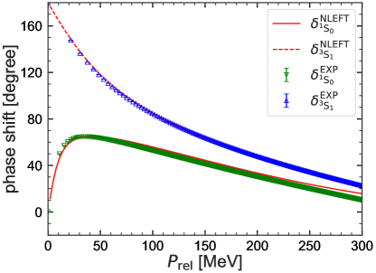
Figure 3: Plots of the neutron-proton scattering phase shifts as functions of relative momenta. The blue up-triangles and green down-triangles denote the ${}^{3}{\rm S}_{1}$ and ${}^{1}{\rm S}_{0}$ phase shifts extracted from the Nijmegen partial wave analysis Stoks et al. (1993), respectively. The solid and dash-dotted curve represents the lattice results for the ${}^{1}{\rm S}_{0}$ and the ${}^{3}{\rm S}_{1}$ phase shift, in order.

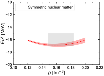
Figure 4: Energy per nucleon as a function of density for symmetric nuclear matter . The gray shaded area indicates the empirical values.

In the next step, we determine the two LECs of the three-nucleon forces given in Eq. (8). This is accomplished by obtaining best fits to the saturation properties of symmetric nuclear matter considering all possible combinations of $d_{1}$ and $d_{2}$ with $0\leq d_{1}<d_{2}\leq 3$. Through this process, we arrive at six distinct interactions, enabling us to quantify the theoretical uncertainty of our calculations. The results for the energy per nucleon in symmetric nuclear matter are illustrated in Fig. 4. The red shaded area represents the variation in energies resulting from different interactions, while the red dashed line denotes the mean value for the energy per nucleon in symmetric nuclear matter, corresponding to the $3N$ interactions with LECs $c_{NNN}^{(1)}=4.98\times 10^{-12}$ MeV^-5 and $c_{NNN}^{(3)}=1.80\times 10^{-12}$ MeV^-5. The gray shaded area denotes the empirical values. As a prediction, we find for the compression modulus $K_{\infty}=229.0(3.6)$ MeV, in good agreement with the empirical value of $K_{\infty}=240(20)$ MeV Garg and Colò (2018). Furthermore, we compute the ground state energies of several light nuclei with $A=3-16$, and our predictions are summarized in Tab. 1. These results are consistent with those reported in Ref. Lu et al. (2019), except for ³H and ⁴He, which were used to constrain the $3N$ force therein.

Table 1: Calculated ground state energies of some light nuclei with $A=3-16$ compared to the empirical values (in MeV). The first and second parentheses denote the statistical error and theoretical error.

Nucleus	NLEFT	Exp.
3H	$-9.21(4)(1)$	$-8.48$
4He	$-29.38(1)(4)$	$-28.3$
8Be	$-58.38(3)(7)$	$-56.5$
12C	$-87.08(12)(11)$	$-92.2$
16O	$-121.84(28)(52)$	$-127.6$

III Hypernuclei

As it is done in the nucleonic sector, to study the EoS of hyper neutron matter, we first determine the unknown LECs of the interactions involving $\Lambda$ hyperons. We start again with the two baryon-interactions. For the $\Lambda N$ interaction, we fit experimental total cross-section data for laboratory momenta below 600 MeV, as shown in the left panel of Fig. 5. Meanwhile, for the $\Lambda\Lambda$ interaction, given the absence of comprehensive cross-section data, we fit to the ${}^{1}{\rm S}_{0}$ phase shift derived from chiral EFT at next-to-leading order Haidenbauer et al. (2016). From these analyses, we determine the coupling constants as $c_{N\Lambda}=-6.52\times 10^{-8}$ MeV^-2 and $c_{\Lambda\Lambda}=-2.96\times 10^{-8}$ MeV^-2.

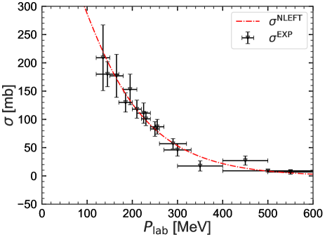
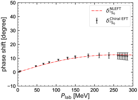
Figure 5: Baryon-baryon interactions. Left Panel: Fit to the cross section for $N\Lambda$ scattering Sechi-Zorn et al. (1968); Alexander et al. (1968); Kadyk et al. (1971); Hauptman et al. (1977). Right Panel: Fit to the $\Lambda\Lambda$ scattering phase shift from chiral EFT Haidenbauer et al. (2016).

Similar to our nucleonic studies, we use hypernuclei to constrain the LECs of $\Lambda NN$ and $\Lambda\Lambda N$ three-baryon forces, more precisely the ground-state energies of single-$\Lambda$ and double-$\Lambda$ hypernuclei. A direct comparison of our calculations with experimental results is given for the separation energy, defined as

$$B_{\Lambda}(_{\Lambda}^{A}Z)=E(^{A-1}Z)-E(_{\Lambda}^{A}Z),$$ (20)

where $E$ is the energy of the system, $A$ its atomic number and $Z$ its charge. The computation of $B$ thus involves the calculation of the energy of the nucleus ${}^{A-1}Z$ and the corresponding hypernucleus ${}_{\Lambda}^{A}Z$. In the case of double-$\Lambda$ hypernuclei, the interesting observable we can access with the NLEFT is the double separation energy,

$$B_{\Lambda\Lambda}(_{\Lambda\Lambda}^{A}Z)=E(^{A-2}Z)-E(_{\Lambda\Lambda}^{A}Z)~{}.$$ (21)

The calculation of this observable proceeds in the same way in the case single-$\Lambda$ hypernuclei, starting from the energy of the nucleus, the corresponding $\Lambda$ hypernucleus and now the double-$\Lambda$ hypernucleus. The results for the separation energies for the various single-$\Lambda$ and double-$\Lambda$ hypernuclei are collected in Tab. 2.

Table 2: $\Lambda$ separation energies for single-$\Lambda$ and double-$\Lambda$ hypernuclei (in MeV). The first error is the statistical one whereas the second error is the systematic one (due to the three-baryon forces). The ^∗ marks a prediction.

System	NLEFT	Exp.
${}_{\Lambda}^{5}$He	$3.40(1)(1)$	$3.10(3)$
${}_{\Lambda}^{9}$Be	$5.72(5)(4)$	$6.61(7)$
${}_{\Lambda}^{13}$C	$10.54(17)(29)^{*}$	$11.80(16)$
${}_{\Lambda\Lambda}^{6}$He	$7.36(1)(4)$	$6.91(16)$
${}_{\Lambda\Lambda}^{10}$Be	$13.30(7)(12)$	$14.70(40)$
${}_{\Lambda\Lambda}^{12}$Be	$21.22(56)(21)^{*}$	$21.48(121)$

As discussed in the main text, these parameters define the HNM(I) approach, which leads to a maximum neutron star mass of $1.52(1)(1)\,M_{\odot}$. To achieve a stiffer EoS, we must increase the strength of the three-body forces but including some data point corresponding to a heavy system. We chose the maximum mass of a neutron star as this data point. With $M_{\rm max}=1.93(1)(1)$ and $2.12(1)(2)$ we obtain HNM(II) and HNM(III), respectively. As discussed before, for HNM(I), the couplings $c_{NN\Lambda}$ and $c_{N\Lambda\Lambda}$ are determined by the hyper-nuclei. For HNM(II), the LECs are $1.8\times c_{NN\Lambda}$ and $4.2\times c_{N\Lambda\Lambda}$, and for HNM(III), these LECs are $2.3\times c_{NN\Lambda}$ and $6.0\times c_{N\Lambda\Lambda}$. See also the discussion in Sec. V.

IV Neutron star EoS and neutron star properties

In this section we start by giving expressions derived using the equations of state and properties of neutron stars as well as by focusing on the behavior of hyper-neutron matter (HNM) comprising both neutrons and $\Lambda$ hyperons. HNM consists of neutrons and a fraction of $\Lambda$ hyperons defined as $x_{\Lambda}=\rho_{\Lambda}/\rho$, where $\rho=\rho_{N}+\rho_{\Lambda}$ represents the total baryon density of the system. Therefore, the neutron and hyperon densities are written as $\rho_{N}=(1-x_{\Lambda})\rho$ and $\rho_{\Lambda}=\rho x_{\Lambda}$, respectively. The HNM energy per particle can be expressed as

$$e_{\rm HNM}(\rho,x_{\Lambda})=\frac{E_{\rm HNM}(\rho,x_{\Lambda})}{N_{\rm tot}}+m_{N}(1-x_{\Lambda})+m_{\Lambda}x_{\Lambda},$$ (22)

where $E_{\rm HNM}(\rho,x_{\Lambda})$ and $N_{\rm tot}=N_{N}+N_{\Lambda}$ denote the total energy of HNM and the total number of baryons, respectively. $m_{N}$ and $m_{\Lambda}$ are the mass for neutrons and $\Lambda$ hyperons as defined in Sec. I.1. Now, our objective is to compute $e_{\scriptscriptstyle\rm HNM}(\rho,x_{\Lambda})$, and subsequently, calculate the energy density $\varepsilon_{\scriptscriptstyle\rm HNM}$, defined as $\varepsilon_{\scriptscriptstyle\rm HNM}=\rho e_{\scriptscriptstyle\rm HNM}$. The chemical potentials for neutrons and hyperons, denoted by $\mu_{N}(\rho,x_{\Lambda})$ and $\mu_{\Lambda}(\rho,x_{\Lambda})$ respectively, are then evaluated using the expressions,

$$\mu_{N}(\rho,x_{\Lambda})=\frac{\partial\varepsilon_{\scriptscriptstyle\rm HNM}}{\partial\rho_{N}},~{}~{}\mu_{\Lambda}(\rho,x_{\Lambda})=\frac{\partial\varepsilon_{\scriptscriptstyle\rm HNM}}{\partial\rho_{\Lambda}}\,.$$ (23)

The hyperon fraction as a function of the baryon density, $x_{\Lambda}(\rho)$, is determined by imposing the condition $\mu_{\Lambda}=\mu_{N}$, which yields the threshold density $\rho_{\Lambda}^{\rm th}$ which is marking the point at which $x_{\Lambda}(\rho)$ first deviates from zero. Finally, the pressure $P(\rho)$ of HNM is obtained from the energy density,

$$P(\rho)=\rho^{2}\frac{d}{d\rho}\frac{\varepsilon_{\scriptscriptstyle\rm HNM}}{\rho}=\sum_{i=N,\Lambda}\rho_{i}\mu_{i}-\varepsilon_{\scriptscriptstyle\rm HNM}.$$ (24)

Once the EoS of PNM and HNM in the form $P(\varepsilon)$ is obtained in Eq. (24), the mass and radius of a neutron star can be described by the Tolman-Oppenheimer-Volkoff (TOV) equations Tolman (1939); Oppenheimer and Volkoff (1939)

$$\frac{dP(r)}{dr}= \ -\frac{[P(r)+\varepsilon(r)][M(r)+4\pi r^{3}P(r)]}{r[r-2M(r)]},$$ (25a)

$$\frac{dM(r)}{dr}= \ 4\pi r^{2}\varepsilon(r),$$ (25b)

where $P(r)$ is the pressure at radius $r$ and $M(r)$ is the total mass inside a sphere of radius $r$.

Besides the masses and radii, another important property of neutron star, the tidal deformability $\Lambda$, is defined as

$$\Lambda=\frac{2}{3}k_{2}C^{-5},$$ (26)

which represents the mass quadrupole moment response of a neutron star to the strong gravitational field induced by its companion. Further, $C=M/R$ is the compactness parameter, $M$ and $R$ are the neutron star mass and radius, and $k_{2}$ is the second love number

$$k_{2}= \frac{8C^{5}}{5}(1-2C)^{2}[2-y_{R}+2C(y_{R}-1)]\times\{6C[2-y_{R}+C(5y_{R}-8)]$$ (27)

$$+4C^{3}[13-11y_{R}+C(3y_{R}-2)+2C^{2}(1+y_{R})]$$

$$+3(1-2C)^{2}[2-y_{R}+2C(y_{R}-1)]\ln(1-2C)\}^{-1},$$

where $y_{R}=y(R)$ can be calculated by solving the following differential equation:

$$r\frac{dy(r)}{dr}+y^{2}(r)+y(r)F(r)+r^{2}Q(r)=0,$$ (28)

with

$$F(r) =\left[1-\frac{2M(r)}{r}\right]^{-1}\times\left\{1-4\pi r^{2}[\varepsilon(r)-P(r)]\right\},$$ (29a)

$$Q(r) =\left\{4\pi\left[5\varepsilon(r)+9P(r)+\frac{\varepsilon(r)+P(r)}{\frac{\partial P}{\partial\varepsilon}(r)}\right]-\frac{6}{r^{2}}\right\}\times\left[1-\frac{2M(r)}{r}\right]^{-1}$$

$$~{}~{}-\left[\frac{2M(r)}{r^{2}}+2\times 4\pi rP(r)\right]^{2}\times\left[1-\frac{2M(r)}{r}\right]^{-2}.$$ (29b)

The differential equation (28) can be integrated together with the TOV equations with the boundary condition $y(0)=2$.

The moment of inertia is calculated under the slow-rotation approximation pioneered by Hartle and Thorne Hartle (1967); Hartle and Thorne (1968), where the frequency $\Omega$ of a uniformly rotating neutron star is significantly lower than the Kepler frequency at the equator, $\Omega\ll\Omega_{\text{max}}\simeq\sqrt{M/R^{3}}$. In the slow-rotation approximation, the moment of inertia of a uniformly rotating, axially symmetric neutron star is given by the following expression Fattoyev and Piekarewicz (2010)

$$I=\frac{8\pi}{3}\int^{R}_{0}r^{4}e^{-\nu(r)}\frac{\bar{\omega}(r)}{\Omega}\frac{\epsilon(r)+P(r)}{\sqrt{1-2M(r)/r}}dr.$$ (30)

The quantity $\nu(r)$ is a radially-dependent metric function and defined as

$$\nu(r)=\frac{1}{2}\ln\left(1-\frac{2M}{R}\right)-\int^{R}_{r}\frac{M(x)+4\pi x^{3}P(x)}{x^{2}[1-2M(x)/x]}dx.$$ (31)

The frame-dragging angular velocity $\bar{\omega}$ is usually obtained by the dimensionless relative frequency $\tilde{\omega}\equiv\bar{\omega}/\Omega$, which satisfies the following second-order differential equation:

$$\frac{d}{dr}\left[r^{4}j(r)\frac{d\tilde{\omega}(r)}{dr}\right]+4r^{3}\frac{dj(r)}{dr}\tilde{\omega}(r)=0,$$ (32)

where $j(r)=e^{-\nu(r)}\sqrt{1-2M(r)/r}$ for $r\leq R$. The relative frequency $\tilde{\omega}(r)$ is subject to the following two boundary conditions

$$\tilde{\omega}^{\prime}(0)= \ 0,$$ (33a)

$$\tilde{\omega}(R)+\frac{R}{3}\tilde{\omega}^{\prime}(R)= \ 1.$$ (33b)

It should be noted that under the slow-rotation approximation, the moment of inertia is independent of the stellar frequency $\Omega$.

The quadrupole moment describes how much a neutron star is deformed away from sphericity due to rotation. It can be computed by numerically solving for the interior and exterior gravitational field of a neutron star in a slow-rotation Hartle (1967); Hartle and Thorne (1968) and a small-tidal-deformation approximation Hinderer (2008); Hinderer et al. (2010). The quadrupole moment in this work is calculated by following the detailed instructions described in Ref. Yagi and Yunes (2013b). To explore the universal $I$-Love-$Q$ relations, the following dimensionless quantities are introduced

$$\bar{I}\equiv\frac{I}{M^{3}},\qquad\bar{Q}\equiv-\frac{QM}{(I\Omega)^{2}}.$$ (34)

V Further equation of state and neutron star properties

Here, we collect some further results on neutron star properties. First, we consider the EoS state in the form $P(\epsilon)$ as given in Fig. 6 (left panel). Second, we display the tidal deformability $\Lambda$ versus the neutron star mass in Fig. 6 (right panel) in comparison to the deduced values from neutron star mergers. Third, in Fig. 7 we display the $Q$-Love and the $I$-$Q$ relation, respectively. The corresponding values for the corresponding fit formulas are collected in Table 3.

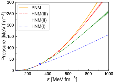
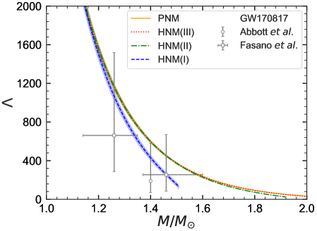
Figure 6: Left Panel: Pressure as a function of energy density. Shown are the results for pure neutron matter as well as the three hyper-neutron matter equations of state considered here. Right Panel: Neutron star tidal deformability, $\Lambda$, as a function of neutron star mass. $\Lambda(M)$ is compared to the masses and tidal deformabilities inferred in Ref. Fasano et al. (2019) for the two neutron stars in the merger event GW170817 at the 90% level (open squares) as well as $\Lambda(1.4M_{\odot})$ at the 90% level extracted from GW170817 Abbott et al. (2018) (open circle).

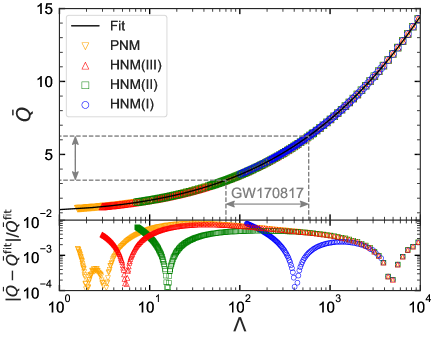
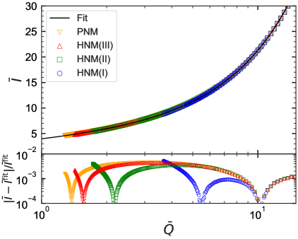
Figure 7: Left Panel: The $Q$-Love relation. Right Panel: The $I$-$Q$ relation.

Table 3: Numerical coefficients for the fit formula of the $I$-Love, $I$-$Q$, and $Q$-Love relations.

$y_{i}$	$x_{i}$	$a_{i}$	$b_{i}$	$c_{i}$	$d_{i}$	$e_{i}$
$\bar{I}$	$\Lambda$	$1.49093\times 10^{0}$	$5.93880\times 10^{-2}$	$2.24914\times 10^{-2}$	$-6.93727\times 10^{-4}$	$7.78146\times 10^{-6}$
$\bar{Q}$	$\Lambda$	$1.97175\times 10^{-1}$	$9.19620\times 10^{-2}$	$4.93555\times 10^{-2}$	$-4.56214\times 10^{-3}$	$1.39647\times 10^{-4}$
$\bar{I}$	$\bar{Q}$	$1.40269\times 10^{0}$	$5.25610\times 10^{-1}$	$4.07856\times 10^{-2}$	$1.85656\times 10^{-2}$	$1.00574\times 10^{-4}$

Next, we discuss the relative importance of the $(\Lambda\Lambda+N\Lambda\Lambda)$ with $S=-2$ with respect to the $(N\Lambda+NN\Lambda)$ interaction with $S=-1$. To evaluate their impact, we switch off the $S=-2$ part for HNM(I) as shown in Fig. 8. While the threshold density where $\Lambda$s start to appear is entirely given by the $S=-1$ interactions, it can be seen that at higher energies (or densities), the $S=-2$ interaction becomes more important. Notably, the maximum neutron star mass changes from $1.52(1)(1)M_{\odot}$ to $1.42(1)(1)M_{\odot}$ when the $S=-2$ interactions are switched off. This observation also explains that we use different scaling factors for $NN\Lambda$ and $N\Lambda\Lambda$ interactions in the construction of HNM(II) and HNM(III) as to make the EoS stiffer beyond the $\Lambda$ threshold is easily done by increasing the $S=-2$ interaction. This is very different from earlier investigations that simply ignored this type of interaction.

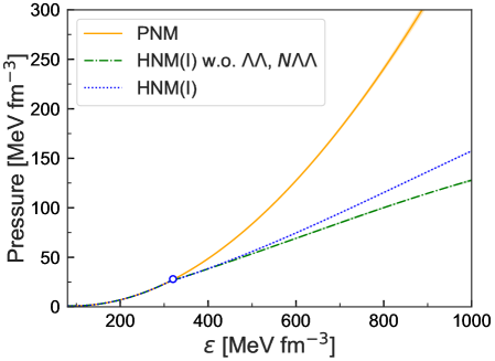
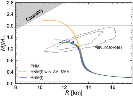
Figure 8: Left Panel: Pressure as a function of energy density. We show PNM (solid orange line) and HNM(I) (dotted blue line). The green dot-dashed line shows the resulting pressure when the $S=-2$ interactions, namely $\Lambda\Lambda$ and $N\Lambda\Lambda$ are switched off. Right Panel: Mass-radius relation. The lines are the same as in the left panel.

VI Comparisons to other calculations

Here, we will compare our calculations with a few other ones, which we consider as benchmarks. We will restrict ourselves to purely baryonic scenarios. We are well aware of attempts to use beyond the standard model physics or modified gravity in this context, but a meaningful comparison to such work can only be done in review article.

First, we compare our work to the pioneering calculations of Lonardoni et al. Lonardoni et al. (2015). They perform auxiliary field diffusion Monte Carlo (AFDMC) simulations with $N_{n}=38,54,66$ neutrons. For the nucleonic sector, they use the phenomenological well-motivated AV8’ and Urbana IX two- and three-body forces. We note that their PNM EoS is stiffer than ours and violates the causality limit for the speed of sound above $\rho\simeq 0.68$ fm^-3, see the left panel of Fig. 9. They perform calculations with $N_{\Lambda}=1,2,14$ hyperons and use a phenomenological hyperon-nucleon potential based on the work of Bodmer et al. (1984). The EoS of HNM is then obtained with an extrapolation function $f(\rho,x_{\Lambda})$, which is quadratic in density and cubic in the $\Lambda$-fraction $x_{\Lambda}$. Clearly, in this respect our calculation is superior in that we cover the whole range of densities and $\Lambda$-fractions relevant to the problem at hand. The $\Lambda$-fraction in their calculation is larger at higher densities for the parametrizations (I) of the $NN\Lambda$ force that predict for neutron star maximum mass to $1.36(5)M_{\odot}$, see the right panel of Fig. 9. Also, the $\Lambda$-fraction is zero at higher densities for the parametrizations (II) of the $NN\Lambda$ force that allow for neutron star masses above $2M_{\odot}$.

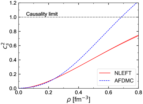
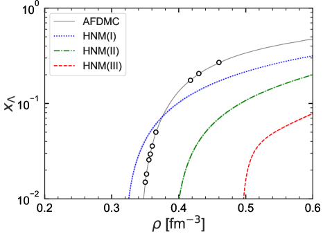
Figure 9: Left Panel: Speed of sound as a function of density for the pure neutron matter. The red solid curve is obtained from our calculations. The blue dashed curve are calculated with the two-nucleon interaction Argonne V8’ (AV8’) potential and the Urbana IX (UIX) three-body potential from the AFDMC Lonardoni et al. (2015). The dot-dashed line represents the causality limit $c_{s}^{2}=1$. Right Panel: Lambda fractions for our three HNM EoSs and the one from AFDMC Lonardoni et al. (2015). The black circles denote a different number of neutrons $(N_{n}=66,54,38)$ and hyperons $(N_{\Lambda}=1,2,14)$ in the simulation box giving momentum closed shells in AFDMC.

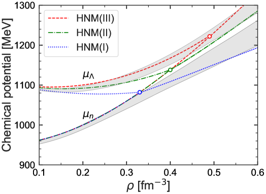
Figure 10: The chemical potential for neutrons and $\Lambda$ hyperons. The gray shaded area indicates the values by using the chiral SU(3) interactions NLO19 with two and three-body forces $(N\Lambda+NN\Lambda)$ Gerstung et al. (2020). The $\Lambda$ threshold densities $\rho_{\Lambda}^{\rm th}$ are marked by open circles. The chemical equilibrium conditions, $\mu_{\Lambda}=\mu_{n}$, are fulfilled above $\rho_{\Lambda}^{\rm th}$ .

Next, we compare our work with the one of Gerstung et al. Gerstung et al. (2020). For the $\Lambda N$ interaction, they consider two next-to-leading order chiral EFT representations, called NLO13 Haidenbauer et al. (2013) and NLO19 Haidenbauer et al. (2020). For the three-body forces, they use the leading $\Lambda NN$ representation based on chiral EFT (contact terms, one-pion and two-pion exchanges) with the inclusion of the $\Lambda NN\leftrightarrow\Sigma NN$ transition Petschauer et al. (2016) in an effective density-dependent two-body approximation Petschauer et al. (2017). The pertinent LECs are given in terms of decuplet resonance saturation and leave one with two $B^{*}BBB$ couplings, where $B$ denotes the baryon octet and $B^{*}$ the decuplet. If one only considers the $\Lambda NN$ force as we do, these two LECs appear in the combination $H^{\prime}=H_{1}+H_{2}$. No $\Lambda\Lambda N$ force was considered in Gerstung et al. (2020). The two LECs $H_{1},H_{2}$ where constrained inGerstung et al. (2020) so that the $\Lambda$ single-particle potential in infinite matter is $U_{\Lambda}(\rho\simeq\rho_{0})=-30$ MeV Gal et al. (2016). Due to numerical instabilities in calculation of the Brueckner $G$-matrix, the computation can only be done up to densities $\rho\simeq 3.5\rho_{0}$. The authors of Ref. Gerstung et al. (2020) then use a quadratic polynomial to extrapolate to higher densities. They calculate the chemical potential for the neutrons and $\Lambda$s from the Gibbs-Duhem relation using a microscopic EoS computed from a chiral nucleon-meson field theory in combination with functional renormalization group methods. The parameter combinations $(H_{1},~{}H_{2})$ were chosen so that the $\Lambda$ single-particle potential becomes maximally repulsive at higher densities. The resulting chemical potentials are displayed in Fig. 10 for the NLO19 $\Lambda N$ forces. These agree well with the HNM(III) chemical potentials up to $\rho\simeq 2.5\rho_{0}$ but show, different to what we find, no crossing. Note that the forces discussed in Gerstung et al. (2020) have not been applied to finite nuclei.

References

- Abbott et al. (2017) B. P. Abbott et al. (LIGO Scientific, Virgo), Phys. Rev. Lett. 119, 161101 (2017), eprint 1710.05832.
- Abbott et al. (2018) B. P. Abbott et al. (LIGO Scientific, Virgo), Phys. Rev. Lett. 121, 161101 (2018), eprint 1805.11581.
- Huth et al. (2022) S. Huth et al., Nature 606, 276 (2022), eprint 2107.06229.
- Lattimer and Prakash (2004) J. M. Lattimer and M. Prakash, Science 304, 536 (2004), eprint astro-ph/0405262.
- Gal et al. (2016) A. Gal, E. V. Hungerford, and D. J. Millener, Rev. Mod. Phys. 88, 035004 (2016), eprint 1605.00557.
- Burgio et al. (2021) G. F. Burgio, H. J. Schulze, I. Vidana, and J. B. Wei, Prog. Part. Nucl. Phys. 120, 103879 (2021), eprint 2105.03747.
- Djapo et al. (2010) H. Djapo, B.-J. Schaefer, and J. Wambach, Phys. Rev. C 81, 035803 (2010), eprint 0811.2939.
- Vidana et al. (2011) I. Vidana, D. Logoteta, C. Providencia, A. Polls, and I. Bombaci, EPL 94, 11002 (2011), eprint 1006.5660.
- Schulze and Rijken (2011) H. J. Schulze and T. Rijken, Phys. Rev. C 84, 035801 (2011).
- Lonardoni et al. (2015) D. Lonardoni, A. Lovato, S. Gandolfi, and F. Pederiva, Phys. Rev. Lett. 114, 092301 (2015), eprint 1407.4448.
- Astashenok et al. (2014) A. V. Astashenok, S. Capozziello, and S. D. Odintsov, Phys. Rev. D 89, 103509 (2014), eprint 1401.4546.
- Chatterjee and Vidaña (2016) D. Chatterjee and I. Vidaña, Eur. Phys. J. A 52, 29 (2016), eprint 1510.06306.
- Maslov et al. (2015) K. A. Maslov, E. E. Kolomeitsev, and D. N. Voskresensky, Phys. Lett. B 748, 369 (2015), eprint 1504.02915.
- Haidenbauer et al. (2017) J. Haidenbauer, U.-G. Meißner, N. Kaiser, and W. Weise, Eur. Phys. J. A 53, 121 (2017), eprint 1612.03758.
- Masuda et al. (2016) K. Masuda, T. Hatsuda, and T. Takatsuka, Eur. Phys. J. A 52, 65 (2016), eprint 1508.04861.
- Logoteta et al. (2019) D. Logoteta, I. Vidana, and I. Bombaci, Eur. Phys. J. A 55, 207 (2019), eprint 1906.11722.
- Gerstung et al. (2020) D. Gerstung, N. Kaiser, and W. Weise, Eur. Phys. J. A 56, 175 (2020), eprint 2001.10563.
- Friedman and Gal (2023) E. Friedman and A. Gal, Phys. Lett. B 837, 137669 (2023), eprint 2204.02264.
- Lee (2009) D. Lee, Prog. Part. Nucl. Phys. 63, 117 (2009), eprint 0804.3501.
- Lähde and Meißner (2019) T. A. Lähde and U.-G. Meißner, Nuclear Lattice Effective Field Theory: An introduction, vol. 957 (Springer, 2019).
- Lu et al. (2019) B.-N. Lu, N. Li, S. Elhatisari, D. Lee, E. Epelbaum, and U.-G. Meißner, Phys. Lett. B 797, 134863 (2019), eprint 1812.10928.
- Pieper and Wiringa (2001) S. C. Pieper and R. B. Wiringa, Ann. Rev. Nucl. Part. Sci. 51, 53 (2001), eprint nucl-th/0103005.
- Hüther et al. (2020) T. Hüther, K. Vobig, K. Hebeler, R. Machleidt, and R. Roth, Phys. Lett. B 808, 135651 (2020), eprint 1911.04955.
- Sechi-Zorn et al. (1968) B. Sechi-Zorn, B. Kehoe, J. Twitty, and R. A. Burnstein, Phys. Rev. 175, 1735 (1968).
- Alexander et al. (1968) G. Alexander, U. Karshon, A. Shapira, G. Yekutieli, R. Engelmann, H. Filthuth, and W. Lughofer, Phys. Rev. 173, 1452 (1968).
- Kadyk et al. (1971) J. A. Kadyk, G. Alexander, J. H. Chan, P. Gaposchkin, and G. H. Trilling, Nucl. Phys. B 27, 13 (1971).
- Hauptman et al. (1977) J. M. Hauptman, J. A. Kadyk, and G. H. Trilling, Nucl. Phys. B 125, 29 (1977).
- Haidenbauer et al. (2016) J. Haidenbauer, U.-G. Meißner, and S. Petschauer, Nucl. Phys. A 954, 273 (2016), eprint 1511.05859.
- Lynn et al. (2016) J. E. Lynn, I. Tews, J. Carlson, S. Gandolfi, A. Gezerlis, K. E. Schmidt, and A. Schwenk, Phys. Rev. Lett. 116, 062501 (2016), eprint 1509.03470.
- Drischler et al. (2019) C. Drischler, K. Hebeler, and A. Schwenk, Phys. Rev. Lett. 122, 042501 (2019), eprint 1710.08220.
- Keller et al. (2023) J. Keller, K. Hebeler, and A. Schwenk, Phys. Rev. Lett. 130, 072701 (2023), eprint 2204.14016.
- Elhatisari et al. (2022) S. Elhatisari et al., accepted for publication in Nature (2022), eprint 2210.17488.
- Brandes et al. (2023) L. Brandes, W. Weise, and N. Kaiser, Phys. Rev. D 108, 094014 (2023), eprint 2306.06218.
- Weber and Weigel (1989) F. Weber and M. K. Weigel, Nucl. Phys. A 505, 779 (1989).
- Balberg and Gal (1997) S. Balberg and A. Gal, Nucl. Phys. A 625, 435 (1997), eprint nucl-th/9704013.
- Tolos et al. (2017) L. Tolos, M. Centelles, and A. Ramos, Astrophys. J. 834, 3 (2017), eprint 1610.00919.
- Baldo et al. (1998) M. Baldo, G. F. Burgio, and H. J. Schulze, Phys. Rev. C 58, 3688 (1998).
- Koehn et al. (2024) H. Koehn et al. (2024), eprint 2402.04172.
- Essick et al. (2021) R. Essick, P. Landry, A. Schwenk, and I. Tews, Phys. Rev. C 104, 065804 (2021), eprint 2107.05528.
- Miller et al. (2019) M. C. Miller et al., Astrophys. J. Lett. 887, L24 (2019), eprint 1912.05705.
- Riley et al. (2021) T. E. Riley et al., Astrophys. J. Lett. 918, L27 (2021), eprint 2105.06980.
- Lattimer and Prakash (2007) J. M. Lattimer and M. Prakash, Phys. Rept. 442, 109 (2007), eprint astro-ph/0612440.
- Tolman (1939) R. C. Tolman, Phys. Rev. 55, 364 (1939).
- Oppenheimer and Volkoff (1939) J. R. Oppenheimer and G. M. Volkoff, Phys. Rev. 55, 374 (1939).
- Demorest et al. (2010) P. Demorest, T. Pennucci, S. Ransom, M. Roberts, and J. Hessels, Nature 467, 1081 (2010), eprint 1010.5788.
- Fonseca et al. (2016) E. Fonseca et al., Astrophys. J. 832, 167 (2016), eprint 1603.00545.
- Arzoumanian et al. (2018) Z. Arzoumanian et al. (NANOGrav), Astrophys. J. Suppl. 235, 37 (2018), eprint 1801.01837.
- Antoniadis et al. (2013) J. Antoniadis et al., Science 340, 6131 (2013), eprint 1304.6875.
- Cromartie et al. (2019) H. T. Cromartie et al. (NANOGrav), Nature Astron. 4, 72 (2019), eprint 1904.06759.
- Fonseca et al. (2021) E. Fonseca et al., Astrophys. J. Lett. 915, L12 (2021), eprint 2104.00880.
- Fasano et al. (2019) M. Fasano, T. Abdelsalhin, A. Maselli, and V. Ferrari, Phys. Rev. Lett. 123, 141101 (2019), eprint 1902.05078.
- Fattoyev et al. (2018) F. J. Fattoyev, J. Piekarewicz, and C. J. Horowitz, Phys. Rev. Lett. 120, 172702 (2018), eprint 1711.06615.
- Annala et al. (2018) E. Annala, T. Gorda, A. Kurkela, and A. Vuorinen, Phys. Rev. Lett. 120, 172703 (2018), eprint 1711.02644.
- Most et al. (2018) E. R. Most, L. R. Weih, L. Rezzolla, and J. Schaffner-Bielich, Phys. Rev. Lett. 120, 261103 (2018), eprint 1803.00549.
- Abbott et al. (2019) B. P. Abbott et al. (LIGO Scientific, Virgo), Phys. Rev. X 9, 011001 (2019), eprint 1805.11579.
- Hebeler et al. (2013) K. Hebeler, J. M. Lattimer, C. J. Pethick, and A. Schwenk, Astrophys. J. 773, 11 (2013), eprint 1303.4662.
- Greif et al. (2020) S. K. Greif, K. Hebeler, J. M. Lattimer, C. J. Pethick, and A. Schwenk, Astrophys. J. 901, 155 (2020), eprint 2005.14164.
- Yagi and Yunes (2013a) K. Yagi and N. Yunes, Science 341, 365 (2013a), eprint 1302.4499.
- Yagi and Yunes (2013b) K. Yagi and N. Yunes, Phys. Rev. D 88, 023009 (2013b), eprint 1303.1528.
- Yagi and Yunes (2017) K. Yagi and N. Yunes, Phys. Rept. 681, 1 (2017), eprint 1608.02582.
- Sedrakian et al. (2023) A. Sedrakian, J.-J. Li, and F. Weber, Prog. Part. Nucl. Phys. 131, 104041 (2023), eprint 2212.01086.
- Li et al. (2023) J. J. Li, A. Sedrakian, and F. Weber, Phys. Rev. C 108, 025810 (2023), eprint 2306.14190.
- Landry and Kumar (2018) P. Landry and B. Kumar, Astrophys. J. Lett. 868, L22 (2018), eprint 1807.04727.
- Wang et al. (2022) S. Wang, C. Wang, and H. Tong, Phys. Rev. C 106, 045804 (2022), eprint 2206.08579.
- Borasoy et al. (2006) B. Borasoy, H. Krebs, D. Lee, and U.-G. Meißner, Nucl. Phys. A 768, 179 (2006), eprint nucl-th/0510047.
- Lee and Schäfer (2005) D. Lee and T. Schäfer, Phys. Rev. C 72, 024006 (2005), eprint nucl-th/0412002.
- Epelbaum et al. (2011) E. Epelbaum, H. Krebs, D. Lee, and U.-G. Meißner, Phys. Rev. Lett. 106, 192501 (2011), eprint 1101.2547.
- Elhatisari et al. (2015) S. Elhatisari, D. Lee, G. Rupak, E. Epelbaum, H. Krebs, T. A. Lähde, T. Luu, and U.-G. Meißner, Nature 528, 111 (2015), eprint 1506.03513.
- Wigner (1937) E. Wigner, Phys. Rev. 51, 106 (1937).
- Lu et al. (2020) B.-N. Lu, N. Li, S. Elhatisari, D. Lee, J. E. Drut, T. A. Lähde, E. Epelbaum, and U.-G. Meißner, Phys. Rev. Lett. 125, 192502 (2020), eprint 1912.05105.
- Ren et al. (2024) Z. Ren, S. Elhatisari, T. A. Lähde, D. Lee, and U.-G. Meißner, Phys. Lett. B 850, 138463 (2024), eprint 2305.15037.
- Shen et al. (2021) S. Shen, T. A. Lähde, D. Lee, and U.-G. Meißner, Eur. Phys. J. A 57, 276 (2021), eprint 2106.04834.
- Shen et al. (2023) S. Shen, S. Elhatisari, T. A. Lähde, D. Lee, B.-N. Lu, and U.-G. Meißner, Nature Commun. 14, 2777 (2023), eprint 2202.13596.
- Meißner et al. (2024) U.-G. Meißner, S. Shen, S. Elhatisari, and D. Lee, Phys. Rev. Lett. 132, 062501 (2024), eprint 2309.01558.
- König et al. (2017) S. König, H. W. Grießhammer, H. W. Hammer, and U. van Kolck, Phys. Rev. Lett. 118, 202501 (2017), eprint 1607.04623.
- Li et al. (2018) N. Li, S. Elhatisari, E. Epelbaum, D. Lee, B.-N. Lu, and U.-G. Meißner, Phys. Rev. C 98, 044002 (2018), eprint 1806.07994.
- Li et al. (2019) N. Li, S. Elhatisari, E. Epelbaum, D. Lee, B. Lu, and U.-G. Meißner, Phys. Rev. C 99, 064001 (2019), eprint 1902.01295.
- Elhatisari et al. (2016) S. Elhatisari et al., Phys. Rev. Lett. 117, 132501 (2016), eprint 1602.04539.
- Meißner et al. (2002) U.-G. Meißner, J. A. Oller, and A. Wirzba, Annals Phys. 297, 27 (2002), eprint nucl-th/0109026.
- Bour (2009) S. Bour, Hyperon-Nucleon Interactions on the Lattice (University of Bonn, 2009).
- Frame et al. (2020) D. Frame, T. A. Lähde, D. Lee, and U.-G. Meißner, Eur. Phys. J. A 56, 248 (2020), eprint 2007.06335.
- Elhatisari and Lee (2014) S. Elhatisari and D. Lee, Phys. Rev. C 90, 064001 (2014), eprint 1407.2784.
- Hildenbrand et al. (2022) F. Hildenbrand, S. Elhatisari, T. A. Lähde, D. Lee, and U.-G. Meißner, Eur. Phys. J. A 58, 167 (2022), eprint 2206.09459.
- Gursey and Radicati (1964) F. Gursey and L. A. Radicati, Phys. Rev. Lett. 13, 173 (1964).
- Sedrakian et al. (2005) A. Sedrakian, J. Mur-Petit, A. Polls, and H. Muther, Phys. Rev. A 72, 013613 (2005), eprint cond-mat/0504511.
- Zhou et al. (2014) L. Zhou, X. Cui, and W. Yi, Phys. Rev. Lett. 112, 195301 (2014).
- Stoks et al. (1993) V. G. J. Stoks, R. A. M. Klomp, M. C. M. Rentmeester, and J. J. de Swart, Phys. Rev. C 48, 792 (1993).
- Garg and Colò (2018) U. Garg and G. Colò, Prog. Part. Nucl. Phys. 101, 55 (2018), eprint 1801.03672.
- Hartle (1967) J. B. Hartle, Astrophys. J. 150, 1005 (1967).
- Hartle and Thorne (1968) J. B. Hartle and K. S. Thorne, Astrophys. J. 153, 807 (1968).
- Fattoyev and Piekarewicz (2010) F. J. Fattoyev and J. Piekarewicz, Phys. Rev. C 82, 025810 (2010), eprint 1006.3758.
- Hinderer (2008) T. Hinderer, Astrophys. J. 677, 1216 (2008), [Erratum: Astrophys.J. 697, 964 (2009)], eprint 0711.2420.
- Hinderer et al. (2010) T. Hinderer, B. D. Lackey, R. N. Lang, and J. S. Read, Phys. Rev. D 81, 123016 (2010), eprint 0911.3535.
- Bodmer et al. (1984) A. R. Bodmer, Q. N. Usmani, and J. Carlson, Phys. Rev. C 29, 684 (1984).
- Haidenbauer et al. (2013) J. Haidenbauer, S. Petschauer, N. Kaiser, U. G. Meißner, A. Nogga, and W. Weise, Nucl. Phys. A 915, 24 (2013), eprint 1304.5339.
- Haidenbauer et al. (2020) J. Haidenbauer, U. G. Meißner, and A. Nogga, Eur. Phys. J. A 56, 91 (2020), eprint 1906.11681.
- Petschauer et al. (2016) S. Petschauer, N. Kaiser, J. Haidenbauer, U.-G. Meißner, and W. Weise, Phys. Rev. C 93, 014001 (2016), eprint 1511.02095.
- Petschauer et al. (2017) S. Petschauer, J. Haidenbauer, N. Kaiser, U.-G. Meißner, and W. Weise, Nucl. Phys. A 957, 347 (2017), eprint 1607.04307.