Aubry transition with small distortions

Résumé

We show that when the Aubry transition occurs in incommensurately distorted structures, the amplitude of the distortions is not necessarily large as suggested by the standard Frenkel-Kontorova mechanical model. By modifying the shape of the potential in such a way that the mechanical force is locally stronger (i.e. increasing the nonlinearities), the transition may occur at a small amplitude of the potential with small distortions. A “phason” gap then opens, while the phonon spectrum resembles a standard undistorted spectrum at higher energies. This may explain the existence of pinned phases with small distortions as experimentally observed in charge-density waves.

I Introduction

The Aubry transition is an equilibrium phase transition at zero temperature between two distinct incommensurately modulated phases Aubry ; aubry_ledaeron . The two phases differ by their degeneracies. One phase has a continuous degenerate manifold of ground states which allows their sliding at no energy cost. In the other phase, the degeneracy is lifted and the ground state manifold becomes discontinuous (and is the Cantor space of Aubry-Mather aubry_ledaeron ; mather ). The symmetry-related ground states are separated by energy barriers, which make them pinned in space. The Aubry transition may thus be viewed as a pinning transition. It was originally called the transition by breaking of analyticity Aubry ; aubry_ledaeron because the envelope function of the modulation (also called the hull function) changes from continuous in the sliding phase to discontinuous in the pinned phase when nonlinear effects in the model become large enough. Originally, the Aubry transition has been discussed in the one-dimensional mechanical Frenkel-Kontorova model Aubry ; aubry_ledaeron and later in various models where two length scales are in competition AubryQuemerais ; FK ; Peyrard .

The question of its experimental relevance is still largely open. Given the generality of the model, it has been claimed to apply in different contexts. It has been invoked in the question of friction and the possibility to have “superlubric” sliding phases, for example in two rotated graphene planes that may slide one over the other with low friction Dew , at incommensurate boundaries of solids lancon2 or for a tip sliding over a surface either in a stick-slip or continuous manner soco . More recently it has been observed and discussed in artificial systems of cold atoms subjected to a periodic optical potential Bylinskii , or two-dimensional colloidal monolayers Brazda . The first application of Aubry’s theory is to incommensurate charge-density waves ledaeronCDW ; AubryQuemerais , which are pinned in the absence of external electric field monceau_book . It was argued that the observed pinning may be an intrinsic effect and the consequence of the Aubry transition AubryQuemerais . However, the distortions measured experimentally are generally small, of the order of a few percents of the lattice spacing pouget_canadell . On the other hand, in the Aubry pinned phase (above the transition at strong enough coupling), the distortions are predicted to be large. For example, in the Frenkel-Kontorova model, they are typically of the order of tens of percent of the bond length at the transition and even larger deep in the pinned phase AubryQuemerais . This is the same in electronic models of charge-density waves AubryQuemerais ; CQ . This discrepancy in the distortions, of almost an order of magnitude, makes it difficult to reconcile theory and experiment. As a consequence extrinsic sources of pinning, i.e. pinning by impurities, have been invoked to explain charge-density waves, but they may not be necessary. The theoretical issue which we study here by introducing a modified Frenkel-Kontorova model, is to understand whether pinning is necessarily accompanied by large distortions, or, in other words, if it is possible to have an incommensurately distorted phase, with small distortions, yet pinned.

The question of disentangling distortions and pinning is not simple as both occur as consequences of the presence of the nonlinear potential in the standard Frenkel-Kontorova model. By introducing a second length scale, in competition with the first, the potential distorts the regular structure. At the same time, by breaking the translation symmetry that ensured the existence of the sliding phase, the potential induces pinning. It is further known that the latter occurs above a threshold for the amplitude of the nonlinear potential and the sliding incommensurate phase remains stable as a consequence of the Kolmogorov-Arnold-Moser (KAM) Scott theorem which thus prevents a pinned phase with small distortions.

There are two extreme and opposite situations that we emphasize. First, there are models, such as that of Brazovskii, Dzyaloshinskii and Krichever BDK , which exhibit a form of ’super-stability’: the sliding phase is stable whatever the strength of the nonlinear coupling. It is then impossible to have a pinned phase (a fortiori with small distortions). This behavior is in fact special. It is the consequence of the integrability of the model: once the integrability is broken, the Aubry transition occurs CQ . Second, if the conditions of the KAM theorem are not fulfilled by the nonlinear term, there is no stability and no reason to have a sliding phase at all: the threshold of the Aubry transition must vanish. A first condition is that the derivative of the potential must be everywhere small enough (this means that the perturbation that enters the dynamical system to which KAM applies must be small enough Remark ). If it were locally diverging for example, KAM theorem would not apply. The strategy is therefore to choose a smooth potential which would develop a singularity under deformation in some limit. Several choices are possible (depending on which derivative should be singular, see Remark ) and we will choose the simplest one with a locally large first derivative. By continuity we expect (and this is what we will check) that the threshold of the Aubry transition will be strongly reduced for such modified potentials. As a matter of fact, there has been interest over the years in modifying either the interatomic potentials Milchev ; Morse ; Quapp or the external periodic potentials PeyrardRemoi1 but the present issue has not been discussed.

The paper is organized as follows. In section II, we introduce the modified model that is characterized by an amplitude and a shape parameter that induces locally large derivatives. We study its Aubry transition (i.e. how the pinning is affected) and the distortions both analytically and numerically in section III. This explains that distortions and pinning are two distinct phenomena in general. In section IV, we compute the phason gap that opens up at the transition and compute, more generally, how the phonon spectrum evolves.

II Modification of the Frenkel-Kontorova model

The modified classical Frenkel-Kontorova model we consider here reads

$$W(\{x_{n}\})=\frac{1}{2}\sum_{n}(x_{n+1}-x_{n}-\mu)^{2}+\frac{K}{(2\pi)^{2}}\sum_{n}V_{\alpha}(x_{n}),$$ (1)

where $x_{n}$ are the continuous physical variables and $K$, $\alpha$ and $\mu$ some parameters. $x_{n}$ is typically the position of an atom $n$ constrained to be along a linear chain. In this case, the first term of $W$ is a local approximation of an interatomic potential which has a minimum at $\mu$. $\mu$ can be regarded as tunable, for example by an external applied force. The second term is a periodic substrate potential with an amplitude controlled by $K$. Its period is chosen to be one (that sets the unit of length with no loss of generality),

$$V_{\alpha}(x+1)=V_{\alpha}(x).$$ (2)

The continuous translation invariance in the absence of the potential, $x_{n}\rightarrow x_{n}+\phi$ where $\phi$ is any real number, is now broken by the potential.

Instead of the standard $\cos 2\pi x$ potential, here we consider a simple modification,

$$V_{\alpha}(x) = \frac{\cosh\alpha\cos 2\pi x-1}{\cosh\alpha-\cos 2\pi x},$$ (3)

which depends on a real parameter $\alpha>0$ that controls the shape (see Fig. 1 and some details in the appendix). When $\alpha\rightarrow+\infty$, $V_{\alpha}(x)\rightarrow\cos(2\pi x)$, giving the standard Frenkel-Kontorova model Aubry ; AubryQuemerais ; FK ; Peyrard . When $\alpha\rightarrow 0$, the potential is more strongly peaked at integers. This choice is interesting because its derivative becomes locally large when $\alpha$ is small. Its maximum is indeed given by (see the appendix)

$$V^{\prime}_{\alpha}(x_{0})=\frac{9\pi}{2\sqrt{3}}\frac{1}{\alpha},$$ (4)

in the limit of small $\alpha$, whereas the amplitude of the potential is a constant equal to 2, allowing us to study the effect of a locally large first derivative. This is in contrast with the $\cos 2\pi x$ choice for which the derivative is bounded by $2\pi$. This is the potential introduced by Peyrard and Remoissenet (up to an irrelevant constant term) PeyrardRemoi1 .

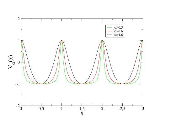
Figure 1: Modified periodic potential $V_{\alpha}(x)$ for various $\alpha$. For large $\alpha$, $V_{\alpha}(x)=\cos(2\pi x)$ (standard Frenkel-Kontorova model). For small $\alpha$, its derivative becomes locally larger.

Its Fourier series is given by

$$V_{\alpha}(x)=1+2\sinh\alpha\sum_{n=0}^{+\infty}e^{-\alpha n}(\cos 2\pi nx-1).$$ (5)

The amplitudes of the successive harmonics decrease exponentially. It can also be viewed as a train of Lorentzians centered on the integers (see the appendix).

We look for the equilibrium configurations $\{x_{n}\}$ that minimize the energy $W(\{x_{n}\})$. They satisfy the equilibrium of forces equation,

$$\frac{\partial W}{\partial x_{n}}=2x_{n}-x_{n-1}-x_{n+1}+\frac{K}{(2\pi)^{2}}V_{\alpha}^{\prime}(x_{n})=0.$$ (6)

Note that if $x_{n}$ is a solution, $x_{n}+k$ where $k$ is any integer is also a solution and $-x_{n}$ too, thanks to the parity of $V_{\alpha}(x)$, $V_{\alpha}(-x)=V_{\alpha}(x)$. It was noticed earlier that, by using the bond lengths $\ell_{n}\equiv x_{n+1}-x_{n}$, the equation can be rewritten as

$$x_{n+1} = x_{n}+\ell_{n}$$ (7)

$$\ell_{n+1} = \ell_{n}+\frac{K}{(2\pi)^{2}}V_{\alpha}^{\prime}(x_{n}+\ell_{n}),$$ (8)

which defines a dynamical system with ’new’ variables determined from the ’old’, $n$ being seen as a discrete time. When $V_{\alpha}(x)$ reduces to the cosine potential, this is the standard map. Iteration of this map starting from given initial configurations gives extremal energy states. Such maps have chaotic unbounded trajectories when $K$ is large enough but also trajectories with well defined average $\langle x_{n+1}-x_{n}\rangle=\ell$ Aubry . We emphasize that the perturbation entering the dynamical system (8) involves the derivative of the potential $\frac{K}{(2\pi)^{2}}V_{\alpha}^{\prime}(x)$ not the potential itself.

III Incommensurate solutions and Aubry transition

We are interested in special solutions with atoms nearly regularly spaced with some distortions, i.e. of the form

$$x_{n}=n\ell+\phi+u_{n},$$ (9)

where $\phi$ is a constant phase and $u_{n}$ some distortions r1 . In the absence of the periodic potential $K=0$, the atomic chain is undistorted, $u_{n}=0$, and the phase $\phi$ is arbitrary. This is the sliding phase of a model with continuous translation symmetry. The quantity $\ell$ is the lattice constant expressed in units of the period of the potential. It is the ratio of the two length scales in competition and may be rational or irrational. When

$$\ell=\frac{r}{s},$$ (10)

where $r$ and $s$ are two coprime integers, we have a repeat of the positions simply translated by $r$,

$$x_{n+s}=x_{n}+r,$$ (11)

i.e. a periodic $u_{n}$ with period $s$, $u_{n+s}=u_{n}$. In that case, the ground state has a unit-cell of size $r$ inside which there are $s$ atoms with positions $x_{n}$ ($n=1,\dots,s$). Below we are interested in incommensurate solutions for which $\ell$ is an irrational number. Physically, it can be viewed as a commensurate solution with a very large period $s$.

We know that, quite generally, the incommensurate sliding phase remains stable, thanks to the KAM theorem which can be applied to the dynamical system [Eqs. 7-8]. The KAM theorem ensures that, if $\ell$ is “sufficiently” irrational (there is a Diophantian condition), the solution (9) at $K=0$, i.e. the sliding phase, is a “stable” trajectory for $K$ small enough (in a sense that we will precise) Remark . The solution for small $K\neq 0$ has now some finite distortions but takes a similar form and can be written

$$x_{n}=n\ell+\phi+g(n\ell+\phi)=f(n\ell+\phi),$$ (12)

involving a function $f$ or $g$ which is continuous. The continuity ensures that it is a simple change of variables and a direct consequence is that $x_{n}\leavevmode\nobreak\$mod 1 continues to take all values in $[0,1]$ just as in the $K=0$ case: the KAM torus (here the circle $[0,1]$) is preserved.

It is known that KAM theorem does not hold for arbitrary large $K$. We will note $K_{c}(\alpha)$ the threshold at which KAM ceases to apply for the modified potential $V_{\alpha}(x)$. This signals the transition to “stochasticity” Greene which is also the Aubry transition between two phases Aubry : for $K<K_{c}(\alpha)$, the sliding phase is stable thanks to KAM theorem. For $K>K_{c}(\alpha)$, KAM theorem does not apply and $g$ is no longer continuous: this is the pinned phase. In fact, the threshold is known very precisely in the case of the standard map and is rather large $K_{c}(\infty)=0.9716$ Greene .

We would like to study here the interplay between the distortions that we will now examine and the pinning determined by $K_{c}(\alpha)$ (section III.3).

III.1 Small $K$

We first consider a perturbation theory at small $K$ to solve (6). We approximate the irrational number $\ell$ by a rational number $\ell=r/s$ (the larger the $s$, the better the approximation). At first order, the energy of the solution (9) with $u_{n}=0$ is simply given by (suppose $\mu=\ell$)

$$\frac{W^{(1)}}{N}=\frac{K}{s(2\pi)^{2}}\sum_{n=1}^{s}V_{\alpha}(n\ell+\phi)=\frac{K}{(2\pi)^{2}}\frac{\sinh\alpha}{\sinh\alpha s}V_{\alpha s}(s\phi)$$ (13)

which goes to zero for all $\phi$ when $s\rightarrow+\infty$ (a consequence of Birkhoff ergodic theorem). It means that the energy barrier for translating the undistorted state by $\phi$ vanishes for an ideal incommensurate state at the lowest order (it is remarkable that it remains true at higher orders as we will see below). Note that for a finite $s$, there are commensuration effects and the extrema are at $\phi=\frac{m}{2s}$ where $m$ is an integer. To determine the distortions $u_{n}=g(n\ell+\phi)$ one may rewrite the extremal condition Eq. (6) as

$$g(x+\ell)+g(x-\ell)-2g(x)=\frac{K}{(2\pi)^{2}}V_{\alpha}^{\prime}(x+g(x)),$$ (14)

where $x=n\ell+\phi$, and use perturbation theory in $K$ to determine the periodic function $g$. By using Fourier series, one formally gets,

$$g(x)=\sum_{p=1}^{+\infty}\frac{A_{p}}{1-\cos(2\pi p\ell)}\sin 2\pi px,$$ (15)

where $A_{p}$ are some coefficients given, at first and second order in $K$, by

$$A_{p}^{(1)} = K\frac{\sinh\alpha}{2\pi}pe^{-\alpha p},$$ (16)

$$A_{p}^{(2)} = K^{2}\frac{\sinh^{2}\alpha}{4\pi}\sum_{n\neq p}\frac{n^{2}(p-n)e^{-\alpha(|n|+|p-n|)}}{1-\cos(2\pi(p-n)\ell)},$$ (17)

where the last sum excludes all $n$ such that $n-p=ks$ where $k$ is an integer, if $\ell=r/s$.

Does the series Eq. (15) converge and what is the amplitude of the distortion?

For rational $\ell=r/s$, $g$ has zero denominators $1-\cos(2\pi p\ell)=0$ when $p$ is a multiple of $s$, $p=ks$, so that (15) is infinite, which means that Eq. (14) cannot be satisfied for all $x$ (or all $\phi$). The only possibility is to choose the special values $\phi=\frac{m}{2s}$ where $m$ is any integer. In this case, when the denominator vanishes (for $p=ks$), the numerator vanishes too: $\sin(2\pi pn\ell+2\pi p\phi)=\sin(2\pi kn+\pi km)=0$. Consequently (14) can be satisfied at these special points but not for all $x$ or all $\phi$, i.e. $g$ is not defined everywhere, as expected for a commensurate solution.

For irrational $\ell$, however, there are “small denominators” but they never vanish. For $\ell$ “sufficiently” irrational (this is where the Diophantian condition is important), it can be shown that the first-order series (15) converges, thanks to the exponential decrease of the harmonics Wayne . The KAM theorem further ensures that higher-order series in $K$ are convergent as well, provided that $K$ remains small enough. In this case, $g$ is a continuous function.

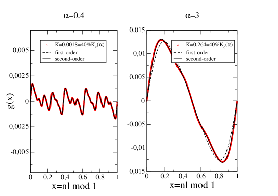
Figure 2: Small $K$. The envelope function $g$ for $K=40\%K_{c}(\alpha)$ is continuous, $\alpha=0.4$ (left) and $\alpha=3$ (right). Numerical and perturbative result in $K$, Eq. 15. Here $\ell=377/987\approx 2-\varphi$.

The amplitude of the distortion is not easy to determine and the naive estimate

$$\delta\sim K\sinh\alpha$$ (18)

from the prefactor of (16) is incorrect because of the small denominators. We now estimate the amplitudes numerically and without relying on perturbation theory.

In Fig. 2, we plot two examples of the numerical computation of $g$ by a steepest descent algorithm which searches a zero of Eq. 6, for two different values of $\alpha$ at small $K$. We compare them with the perturbative results given by Eq. (15) up to second order. We take, as an example, $\ell=\frac{3-\sqrt{5}}{2}=2-\varphi\approx 0.3819660\dots$ ($\varphi$ is the golden number), and we approximate it by $\ell=r/s=377/987=0.3819655$. We have computed numerically all the $x_{n}$ and their distortions $u_{n}$, starting from random values. In the numerical calculation, we obtain $g$ at the special points $x=n\ell\leavevmode\nobreak\$mod 1 (i.e. $s$ points only). We are in principle limited to $K\ll K_{c}(\alpha)$ but take in both cases $K=40\%K_{c}(\alpha)$ to see some deviations from perturbation theory close to the transition. Nevertheless, we observe in both cases ($\alpha=0.4$ on the left and $\alpha=3$ on the right) that the perturbation result is accurate, especially at second-order. Small deviations are visible and disappear for smaller values of $K\ll K_{c}(\alpha)$, or, conversely, are amplified when $K\rightarrow K_{c}(\alpha)$. Note that the $y$ scale is not the same, so that the amplitude of the distortions $\delta$ is much smaller for small $\alpha$ (we have to take smaller values of $K$ as well to remain at a fixed distance from the transition). The shape of the distortions also depends on $\alpha$. When $\alpha\rightarrow+\infty$ (Frenkel-Kontorova) model, only the first harmonic $p=1$ is retained in (15) and $g(x)=\gamma\sin 2\pi x$, $\gamma\equiv\frac{K}{4\pi}\frac{1}{1-\cos 2\pi\ell}$. This is already close to the result for $\alpha=3$. On the other hand, for $\alpha\rightarrow 0$, more and more harmonics must be included, some of them with a large denominator but the result remains small (thanks to smaller $K$). This is what is seen in Fig. 2 (left). The numerical result is thus in agreement with the KAM theorem and well approximated by lowest order perturbation theory.

The distortions are small in this regime and particularly so when $\alpha$ is small and $K$ is appropriately reduced below the transition.

III.2 Large $K$

When $K$ increases further, however, the previous perturbation theory fails. One can consider instead the “anti-integrable” limit $K\rightarrow\infty$ AA and do perturbation theory in $1/K$. At the lowest order in $1/K$, the solutions of Eq. (6) are given by

$$V_{\alpha}^{\prime}(x_{n})=0,$$ (19)

so that $x_{n}$ must be integers or half-integers. Since there is no determination of $x_{n+1}$ from $x_{n}$, any series of integers (or half-integers or a mixing) $x_{n}$ is acceptable, i.e. can be random and very “chaotic”. Among the solutions, the following one,

$$x_{n}=[n\ell]+\frac{1}{2},$$ (20)

where $[\dots]$ is the integer part, is special. Not only all the atoms are at the bottoms of the potential ($x_{n}\leavevmode\nobreak\$mod 1=1/2) which minimize the potential energy (as any series of half integers) but also the average bond length is $\ell$. In this case, the envelope function is simply given by $f(x)=[x]+1/2$. More generally, one can seek a solution in perturbation in $1/K$,

$$f(x)=[x]+\frac{1}{2}+\sum_{n=1}^{\infty}B_{n}([x+n\ell]+[x-n\ell]-2[x]),$$ (21)

with coefficients $B_{n}$ vanishing for large $K$. At first and second order in $1/K$, we find

$$B_{n}^{(1)} = \frac{1}{K}(\frac{1+\cosh\alpha}{\sinh\alpha})^{2}\delta_{n,1},$$ (22)

$$B_{n}^{(2)} = \frac{1}{K^{2}}(\frac{1+\cosh\alpha}{\sinh\alpha})^{4}\delta_{n,2}-\frac{4}{K}B_{n}^{(1)}.$$ (23)

Thus $B_{n}=B_{n}^{(1)}+B_{n}^{(2)}$ (at second order) is a decreasing function of $n$. The perturbation theory is correct if the prefactor is small $\frac{1}{K}(\frac{1+\cosh\alpha}{\sinh\alpha})^{2}\ll 1$, which needs, in the limit of small $\alpha$, that $K\alpha^{2}/4\gg 1$.

In Eq. (21), $f$ is clearly discontinuous at each point $x=\pm n\ell\leavevmode\nobreak\$mod 1 (which are dense in $[0,1]$) with discontinuities that are functions of $B_{n}$. Indeed the periodic function $[x+a]+[x-a]-2[x]=\pm 1,0$ is discontinuous at $\pm a$ and $0$ (and periodic points).

In Fig. 3, the points are the atomic positions $x_{n}$ mod 1 computed numerically for large $K$ and plotted as a function of $n\ell$ mod 1. We thus obtain the graph of $f$ as a function of $x$. For $\alpha=3$ (right figure), the second order result Eq. 21 is shown as well (dashed line) and is a good approximation of the numerical result with main discontinuities at zero (obtained at zeroth order), $\pm\ell$ (first-order) and $\pm 2\ell\leavevmode\nobreak\$mod $1$ (second order). Higher-order discontinuities are not reproduced at this order. The largest discontinuity at zero means that atoms avoid the maxima of the potential. For $\alpha=0.4$ (left figure), the lowest order perturbation theory already fails even for $K=15$ because the prefactor is of order 1. The result shown by a dashed line is a fit that uses (21) and fitting parameters $B_{n}$ up to $n=3$, reproducing the main three discontinuities. The form of the solution (21) seems to remain accurate even though the parameters $B_{n}$ are no longer given by perturbation theory. In both cases, we see that the distortions (departure from the $y=x$ line) are strong,

$$\delta\sim O(1)$$ (24)

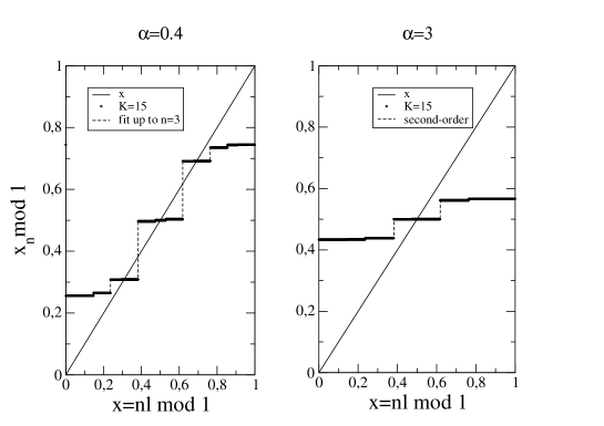
Figure 3: Large $K$. The envelope function $f$ is discontinuous, $\alpha=0.4$ (left) and $\alpha=3$ (right). Numerics and perturbative result in $1/K$, Eq. (21). Here $\ell=377/987\approx 2-\varphi$.

How exactly one interpolates between the two previous regimes $K\rightarrow 0$ and $K\rightarrow\infty$ is through the Aubry transition.

III.3 Aubry transition

The simplest way to show numerically the existence of an Aubry transition is to follow the discontinuities of the envelope functions Aubry ; AubryQuemerais . In Fig. 4, we show, as above, the numerically computed envelope function $f$. Since $K$ is reduced compared with the results of Fig. 3, the distortions are reduced and $f(x)$ gets closer to $f(x)=x$. In each figure, two examples of values of $K$ close to the threshold of the Aubry transition, $K_{c}(\alpha)$, are given. The red points ($K<K_{c}(\alpha)$) are the points of a continuous function (see insets for more clarity), just as in Fig. 2, and the black points ($K>K_{c}(\alpha)$) are that of a discontinuous function as in Fig. 3. We observe that the discontinuities close continuously so that the transition is a second-order transition. Although, strictly speaking, there is no Aubry transition in commensurate systems, using $\ell=r/s=377/987$ with a large $s$ ensures a sharp change of continuity as a function of $K$. By locating the value of $K$ for which the discontinuities close, we extract $K_{c}(\alpha)$ and the phase diagram with the sliding phase $K<K_{c}(\alpha)$ and the pinned phase $K>K_{c}(\alpha)$ (Fig. 5). Note that $K_{c}(\alpha)$ vanishes when $\alpha\rightarrow 0$.

This can be simply understood with an examination of the equilibrium of forces, Eq. (6). At fixed $\ell$ the atoms are constrained to be close enough $|x_{n+1}-x_{n}|<1$ so that the spring forces cannot exceed some value (say 1), and therefore $\frac{K}{(2\pi)^{2}}V_{\alpha}^{\prime}(x_{n})$ cannot be arbitrary large aubry_minor . For irrational $\ell$ and sliding solution $x_{n}$, all values of the derivative are attained somewhere along the chain (because $x_{n}$ mod 1 takes all values in $[0,1]$) in particular its maximum noted $V^{\prime}_{m}$. In the limit of large $\alpha$ ($V^{\prime}_{m}=2\pi$), the equilibrium of forces thus cannot be satisfied once $K>2\pi$ aubry_minor . Similarly, in the limit of small $\alpha$, given the expression of the maximum of the derivative (4), we get that for

$$K>\frac{(2\pi)^{2}}{V^{\prime}_{m}}=\frac{8\pi\sqrt{3}}{9}\alpha\hskip 14.22636pt(\alpha\rightarrow 0),$$ (25)

it is impossible to maintain the balance of forces in a stable sliding phase. In particular, when $\alpha=0$ (corresponding to a singular potential) the right-hand side vanishes so that

$$K_{c}(0)=0$$ (26)

(at the limit $\alpha=0$ the potential is discontinuous at $x=0$ and the KAM torus is destroyed at that point). This qualitative argument confirms that in the limit of small $\alpha$, the pinned phase should be favored at small $K$. Importantly, one sees that if the derivative of the potential $V^{\prime}_{m}$ is somewhere strong enough, the sliding phase no longer exist because the atoms that experience that strong force (some necessarily do in the sliding phase) cannot be at equilibrium: the Aubry transition threshold to the pinned state is reduced. The latter bound is in fact a very crude estimate of $K_{c}(\alpha)$ (see the steep dashed line in Fig. 5). The better bound represented by the dashed curve in Fig. 5 will be given in section IV.

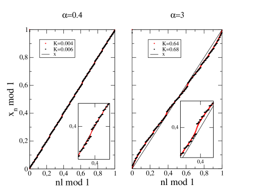
Figure 4: Envelope function $f$ for $\alpha=0.4$ (left) and $\alpha=3$ (right) (zoom in the insets). Red (resp. black) points are for $K<K_{c}(\alpha)$ (resp. $K>K_{c}(\alpha)$) below the Aubry transition (resp. above) and show a continuous function $f$ (resp. discontinuous). Here $\ell=r/s=377/987$. The undistorted result $K=0$ is given by $f(x)=x$.

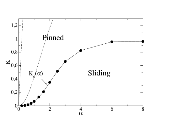
Figure 5: Phase diagram with the sliding and pinned phase separated by the Aubry transition for incommensurate $\ell=2-\varphi$. Dashed lines are simple analytical crude approximants of $K_{c}(\alpha)$, Eqs. (25) and (34).

In order to get some quantitative insights into how large the distortions can be near and at the Aubry transition when the phase is pinned, we also compute numerically the bond lengths,

$$\ell_{n} = \ell+(u_{n+1}-u_{n}).$$ (27)

Recall that the average bond length $\frac{1}{s}\sum_{n=1}^{s}\ell_{n}=\ell$ so that $(u_{n+1}-u_{n})/\ell$ measures the amplitude of the distortion with respect to the average. In Fig. 6, we show that amplitude as a function of $n\ell\leavevmode\nobreak\$mod 1 for $K\sim K_{c}(\alpha)$, which defines another envelope function. Its maximal amplitude

$$\xi\equiv\mbox{Max}|u_{n+1}-u_{n}|/\ell,$$ (28)

gives an idea of how much distorted the structure is. For large values of $\alpha$ ($\alpha=3$ in the right figure), the amplitude is large. On the contrary, for small $\alpha$, we observe that the distortions are well within $1\leavevmode\nobreak\ \%$ of the bond length (the two horizontal lines are at $\pm 1\leavevmode\nobreak\ \%$). The amplitude $\xi$ is reported in Fig. 7 as a function of $\alpha$ at $K=K_{c}(\alpha)$. For large $\alpha$, the maximal distortion at the transition is 23% (Frenkel-Kontorova limit). For smaller values of $\alpha$, $\xi$ can be arbitrary small. This can also be seen qualitatively in Fig. 4 that for small $\alpha$ (left), the distortions are very small and $f$ is very close to the undistorted result $f(x)=x$, whatever the values of $K$ across and near the Aubry transition.

The important conclusion is that it is not necessary to have large distortions to have an Aubry transition or be in the pinned phase. In particular, if $\alpha=0$, so that the potential is discontinuous, $K_{c}(0)=0$ as we have shown above: the system is immediately in the pinned phase. Yet the potential is flat almost everywhere so that there is no distortion. This extreme situation remains somehow valid at small $\alpha$, as shown here: it is replaced by a pinned phase with small distortions.

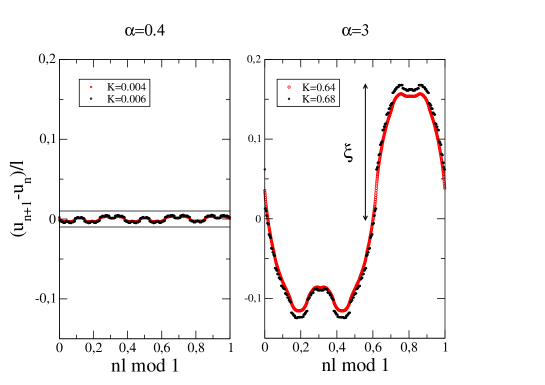
Figure 6: Envelope function $h$ for the normalized bond length across the Aubry transition. The amplitude is noted $\xi$. The horizontal bars on the left show $\pm$ 1%.

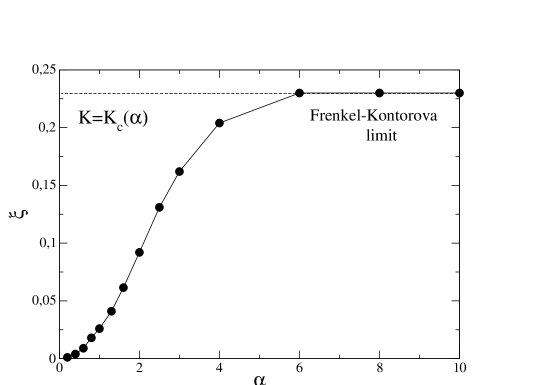
Figure 7: Maximal distortion $\xi$ (see definition in Fig. 6) as a function of the potential shape parameter $\alpha$, at the Aubry transition. At small $\alpha$, $\xi$ can be arbitrarily small and reaches 23% (dashed line) at large $\alpha$ (Frenkel-Kontorova limit).

IV Stability and phonon spectrum

We now examine the stability of the solution and the phonon spectrum, in particular its gap which vanishes at the Aubry transition, defining the zero-energy phason mode of the continuous ground state manifold for $K<K_{c}(\alpha)$. For this, we add the kinetic energy of the atoms

$$H=\frac{1}{2}\sum_{n}\dot{x}_{n}^{2}+W(\{x_{n}\}),$$ (29)

and write

$$x_{n}=x_{n}^{eq}+\epsilon_{n},$$ (30)

where $x_{n}^{eq}=n\ell+u_{n}$ is the equilibrium position in the ground state previously obtained and $\epsilon_{n}$ a sufficiently small deviation to expand the energy:

$$W(\{x_{i}\})=W(\{x_{i}^{eq}\})+\frac{1}{2}\sum_{n,m}\frac{\partial^{2}W}{\partial x_{n}\partial x_{m}}\epsilon_{n}\epsilon_{m}.$$ (31)

The nonzero partial derivatives are given by

$$\frac{\partial^{2}W}{\partial x_{n}^{2}} = 2+\frac{K}{(2\pi)^{2}}V_{\alpha}^{\prime\prime}(x_{n}^{eq}),$$ (32)

$$\frac{\partial^{2}W}{\partial x_{n}\partial x_{n\pm 1}} = -1,$$ (33)

where $x_{n}^{eq}=n\ell+u_{n}$ and $V^{\prime\prime}_{\alpha}(x)$ is the second derivative of the potential given in the appendix. Note that for the equilibrium phase to be a minimum of the energy, the matrix on the right-hand-side of (31) must be definite positive. The (Sylvester) criterion implies in particular that all diagonal elements must be positive aubry_minor . In the sliding phase, all values of $V^{\prime\prime}_{\alpha}(x_{n})$ are attained, in particular its minimum $V^{\prime\prime}_{\alpha}(0)<0$. When $K$ increases, $2+\frac{K}{(2\pi)^{2}}V_{\alpha}^{\prime\prime}(0)$ becomes negative and the matrix is no longer definite positive (the sliding phase is unstable), i.e. when

$$K>\frac{2(2\pi)^{2}}{|V^{\prime\prime}_{\alpha}(0)|}=2\frac{\cosh\alpha-1}{\cosh\alpha+1}$$ (34)

(see 45). This analytical bound is in agreement with (but is crude approximation of) the numerical result giving $K_{c}(\alpha)$ (see the dashed curve in Fig. 5 for a comparison). It could be refined by using higher-order minors aubry_minor but it is not necessary here. We find again the fact that when $\alpha\rightarrow 0$, the sliding phase must be unstable for small $K\lesssim\alpha^{2}/2\rightarrow 0$.

To compute the phonons we now assume a commensurate state with $\ell=r/s$ and that $\epsilon_{n}=\bar{\epsilon}_{n}e^{i(kn-\omega_{k}t)}$ (the amplitude $\bar{\epsilon}_{n}$ is periodic with period $s$) and obtain an $s\times s$ matrix:

$$M_{n,m}=-\omega_{k}^{2}\delta_{n,m}+\frac{\partial^{2}W}{\partial x_{n}\partial x_{m}}.$$ (35)

The matrix $M$ has also the nonzero end points $\frac{\partial^{2}W}{\partial x_{s}\partial x_{1}}=-e^{\pm iks}$ for $\ell\neq 0,1/2$. The diagonalization of $M$ gives the phonon energies $\omega(k)$. For the integrable point $K=0$, the spectrum is simply given by the standard expression:

$$\omega(k)=2|\sin\frac{k}{2}|.$$ (36)

In the opposite anti-integrable limit $K\rightarrow+\infty$, when the atoms are all at the bottoms of the potential, $V^{\prime\prime}_{\alpha}(x_{n})=V^{\prime\prime}_{\alpha}(1/2)$ and the dispersion relation is

$$\omega(k)=\sqrt{\Delta^{2}+4\sin^{2}\frac{k}{2}},$$ (37)

with the gap $\Delta$ given by $\Delta^{2}=\frac{K}{(2\pi)^{2}}V^{\prime\prime}_{\alpha}(1/2)=K\frac{\sinh^{2}\alpha}{(1+\cosh\alpha)^{2}}$ (see (46)). Note that the anti-integrable limit applies precisely when $\Delta\gg 1$ (see section III.2). The spectrum consists in this case of a single (gapped) band.

In between, for $K\neq 0$, the spectrum $\omega(k)$ is computed numerically. Two examples are given in Fig. 8 for $\ell=377/987\approx 2-\varphi$ and two different values of $\alpha$. $\omega(k)$ is represented in half the extended Brillouin zone, i.e. for $k$ in $[0,\pi]$.

In both cases the spectra of the sliding phases ($K<K_{c}(\alpha)$, red curves) have no zero energy gap. This is the consequence of the existence of a continuous manifold of ground states. The associated zero-energy mode is the ’phason’, which becomes gapped in the pinned phase above the Aubry transition $K>K_{c}(\alpha)$ (black curves). Note that, in the two figures, the parameters $K$ in gapped cases are chosen so that the gap is the same (see the black curves in the insets). The values of $K$ (0.008 and 0.71) differ by almost two orders of magnitude. Measuring experimentally a certain gap is therefore not sufficient to tell what the amplitude $K$ of the potential is.

For small $\alpha$ (top), the distortions and the values of $K$ at the Aubry transition are small, so that the spectrum is very close to (36). For large $\alpha$ (bottom), there are much larger gaps at higher energies. Since the periodic potential mixes modes with $k$ and $k\pm 2\pi p\ell$ (where $p$ is an integer) one expects gaps at every level crossing. One sees that for small $\alpha$ the high-energy gaps are all very small while they are large when $\alpha$ is large. This simply reflects the strength of the distortions. It makes a qualitative difference which may help to distinguish experimentally between strongly nonlinear potentials (small $\alpha$) and harmonic potentials (large $\alpha$).

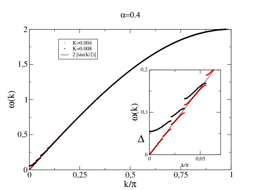
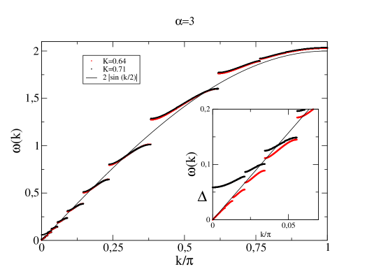
Figure 8: Phonon spectrum for $\alpha=0.4$ and $\alpha=3$ for $K<K_{c}(\alpha)$ (red curves) and $K>K_{c}(\alpha)$ (black curves) (zoom in the insets): opening of the zero-energy gap at $k=0$ at the Aubry transition. $\ell=377/987$.

V Conclusion

The distortions of incommensurately modulated phases are not necessarily as strong as what the Frenkel-Kontorova model or charge-density wave models suggest when pinning occurs. When the smoothness conditions of the nonlinear perturbation are progressively suppressed, i.e. here when the derivative of the potential (the mechanical force) becomes locally strong enough, the pinning threshold $K_{c}(\alpha)$ is reduced. This is because, at the limit, the KAM theorem no longer applies for potentials with some singularities. At the same time, the distortions can be weak if the potential is more flat in large portions of space. This is what we have provided evidence for by considering a simple modified potential in which these two regions coexist, a situation that does not occur in the standard Frenkel-Kontorova model where the derivative of the potential is bounded. The two effects -pinning and distortions- are therefore not necessarily related. This opens a wide range of applicability of the Aubry transition since distortions need not be large in incommensurate pinned phases.

We emphasize that therefore observing experimentally small incommensurate distortions $\xi$ (as in charge-density waves) does not generally imply that the phase should be sliding (this is only true for the standard Frenkel-Kontorova model). It does not imply either that perturbation theory (which leads to the sliding phase) is applicable because it is highly “resonant” due to the “small denominators”. The small parameter of the perturbation theory is $K/K_{c}(\alpha)$, not $\xi$ (so $\xi$ may be small with a large $K/K_{c}(\alpha)$). It is only for the standard Frenkel-Kontorova model that we have simultaneously $\xi\ll 1$ and $K/K_{c}\ll\leavevmode\nobreak\ 1$.

Annexe A Modified potential

The modified potential considered here depends on a real parameter $\alpha$ and is written in three different forms:

$$V_{\alpha}(x) = \frac{\cosh\alpha\cos 2\pi x-1}{\cosh\alpha-\cos 2\pi x}$$ (38)

$$= 1+2\sinh\alpha\sum_{n=0}^{+\infty}e^{-\alpha n}(\cos 2\pi nx-1)$$ (39)

$$= \sum_{n=-\infty}^{+\infty}\frac{2\alpha\sinh\alpha}{[2\pi(x-n)]^{2}+\alpha^{2}}-\cosh\alpha.$$ (40)

It is easy to prove these equalities. For example, starting from (40) and using Poisson’s formula for $h(x)\equiv\frac{\alpha}{4\pi^{2}x^{2}+\alpha^{2}}$,

$$\sum_{n=-\infty}^{+\infty}h(x-n)=\sum_{p=-\infty}^{\infty}\hat{c}_{p}e^{2ip\pi x}$$ (41)

with

$$\hat{c}_{p}=\int_{-\infty}^{+\infty}h(x)e^{-2i\pi px}dx=\frac{1}{2}e^{-|p|\alpha},$$ (42)

we find (39). Then, by resummation of the Fourier series (39), we get (38).

The first and second derivatives of the potential are given by

$$V_{\alpha}^{\prime}(x) = -2\pi\frac{\sinh^{2}\alpha\sin 2\pi x}{(\cosh\alpha-\cos 2\pi x)^{2}}.$$ (43)

$$V_{\alpha}^{\prime\prime}(x)/(2\pi)^{2}=\sinh^{2}\alpha\frac{1+\sin^{2}2\pi x-\cosh\alpha\cos 2\pi x}{(\cosh\alpha-\cos 2\pi x)^{3}}.$$ (44)

The first derivative has a maximum which, for small $\alpha$ for example, is at $x_{0}=\alpha/(2\pi\sqrt{3})$, so that $V^{\prime}_{\alpha}(x_{0})=\frac{9\pi}{2\sqrt{3}}\frac{1}{\alpha}$ which is large when $\alpha$ is small. We also have

$$V_{\alpha}^{\prime\prime}(0)/(2\pi)^{2} = -\frac{\cosh\alpha+1}{\cosh\alpha-1}$$ (45)

$$V_{\alpha}^{\prime\prime}(1/2)/(2\pi)^{2} = \frac{\sinh^{2}\alpha}{(1+\cosh\alpha)^{2}}.$$ (46)

- (1) S. Aubry (1978) In: Bishop A.R., Schneider T. (eds) Solitons and Condensed Matter Physics. Springer Series in Solid-State Sciences, vol 8. Springer, Berlin, Heidelberg.
- (2) S. Aubry and P. Y. Le Daeron, Physica D 8, 381 (1983).
- (3) J. N. Mather, Topology 21, 457 (1982).
- (4) S. Aubry and P. Quémerais, in Low Dimensional Electronic Properties of Molybdenum bronzes and Oxides, ed. C. Schlenker, Kluwer Academic Publishers (1989), 295.
- (5) O. M. Braun and Y. S. Kivshar, The Frenkel-Kontorova Model, Concepts, Methods, and Applications, Springer-Verlag (2004).
- (6) T. Dauxois and M. Peyrard, Physics of solitons, Cambridge University Press (2004).
- (7) M. Dienwiebel et al., Phys. Rev. Lett. 92, 126101 (2004).
- (8) F. Lançon, J. Ye, D. Caliste, T. Radetic, A. M. Minor, and U. Dahmen, Nano Letters 10, 695 (2010).
- (9) A. Socoliuc, R. Bennewitz, E. Gnecco, E. Meyer, Phys. Rev. Lett. 92, 134301 (2004).
- (10) A. Bylinskii et al., Nat Mat 15, 717 (2016).
- (11) T. Brazda et al., Phys. Rev. X 8, 011050 (2018).
- (12) P. Y. Le Daeron and S. Aubry, J. Phys. C: Solid State Phys. 16, 4827 (1983).
- (13) P. Monceau (ed.), Electronic Properties of Inorganic Quasi-one Dimensional Compounds, Part A and B, Reidel Publishing Company (1985).
- (14) J.-P. Pouget and E. Canadell, Rep. Prog. Phys. 87, 026501 (2024).
- (15) O. Cépas and P. Quémerais, SciPost 14, 051 (2023).
- (16) See, for example, H. Scott Dumas, The KAM story, a friendly introduction to the content, history and significance of classical Kolmogorov-Arnold-Moser theory, World Scientific (2014).
- (17) S. A. Brazovskii, I. E. Dzyaloshinskii, and I. M. Krichever, Soviet Phys. JETP 56, 1, 212 (1982).
- (18) Other conditions apply, in particular the perturbation must also be ’smooth enough’. If it has some singularities (possibly in higher-order derivatives), the KAM theorem does not apply. To know what the optimal smoothness conditions are, see Ref. Scott .
- (19) A Milchev, Phys. Rev. B 33, 2062 (1986).
- (20) C.-I Chou et al., Phys. Rev. E 57, 2747 (1998).
- (21) W. Quapp and J. M. Bofill, Eur. Phys. J. B 93, 227, (2020).
- (22) M. Peyrard and M. Remoissenet, Phys. Rev. B 26, 2886 (1982).
- (23) There is an implicit constraint for all in (9) which means that must be bounded.
- (24) J. Greene, J. Math. Phys. 20, 118 (1979).
- (25) The proof of the convergence of such series with small denominators and Diophantian conditions is part of KAM theorem, see, for example, Ref. Scott or C. E. Wayne, in Dynamical Systems and Probabilistic Methods in Partial Differential Equations, ed. P. Deift, C. D. Levermore and C. E. Wayne, Lectures in Applied Mathematics, Vol. 31, 3 (1996).
- (26) S. Aubry and G. Abramovici, Physica D 43, 2, 199 (1990).
- (27) S. Aubry, Physica 7D, 240 (1983).