Detecting and Deterring Manipulation in a Cognitive Hierarchy

Abstract

Social agents with finitely nested opponent models are vulnerable to manipulation by agents with deeper reasoning and more sophisticated opponent modelling. This imbalance, rooted in logic and the theory of recursive modelling frameworks, cannot be solved directly. We propose a computational framework, $\aleph$-IPOMDP, augmenting model-based RL agents’ Bayesian inference with an anomaly detection algorithm and an out-of-belief policy. Our mechanism allows agents to realize they are being deceived, even if they cannot understand how, and to deter opponents via a credible threat. We test this framework in both a mixed-motive and zero-sum game. Our results show the $\aleph$ mechanism’s effectiveness, leading to more equitable outcomes and less exploitation by more sophisticated agents. We discuss implications for AI safety, cybersecurity, cognitive science, and psychiatry.

1 Introduction

Deception is omnipresent in human and animal cultures. Humans use various levels of deception, from “white lies” to harmful lies, manipulating the beliefs for their own benefit. To manipulate, a deceiver needs to know which actions create or reinforce false beliefs, and which actions avoid disclosing their true intentions. The capacity of an agent to place itself in somebody else’s shoes is known as Theory of Mind [ToM; Premack and Woodruff, 1978], a key ingredient to successful deception.

ToM encompasses the capacity to simulate others’ actions and beliefs, often recursively. The depth of the recursion is known as an agent’s depth of mentalisation [DoM; Barnby et al., 2023, Frith and Frith, 2021]. This recursive structure, framed using k-level hierarchical ToM [Camerer et al., 2004], guarantees that agents with lower DoM are incapable of making inferences about the intentions of those with higher DoM [Gmytrasiewicz and Doshi, 2005]. Such an ability would suggest that agents had revoked the paradox of self-reference. This limitation, found in all recursive modelling frameworks [Pacuit and Roy, 2017], implies that agents with low DoM are doomed to be manipulated by others with higher DoM. This asymmetry has previously been explored [Doshi et al., 2014, Hula et al., 2018, Alon et al., 2023a, Sarkadi et al., 2021, 2019a], illustrating the various way high DoM agents can take advantage of low DoM agents.

However, all is not lost. Low DoM agents may still notice that the behaviour they observe is inconsistent with the behaviour they expect, even if they lack the wherewithal to understand how or why Hula et al. [2018]. Such a heuristic mismatch warns the victim that they are facing an unmodeled opponent, meaning that they can no longer use their opponent models for optimal planning. By switching to an out-of-belief (OOB) policy, where actions are sampled against their beliefs, they can act defensively, and even deter more competent opponents from trying to manipulate them. For example, an agent might quit a game against their own best interests to avoid what they perceive as “being taken advantage of”, knowing that this will also harm the deceiver.

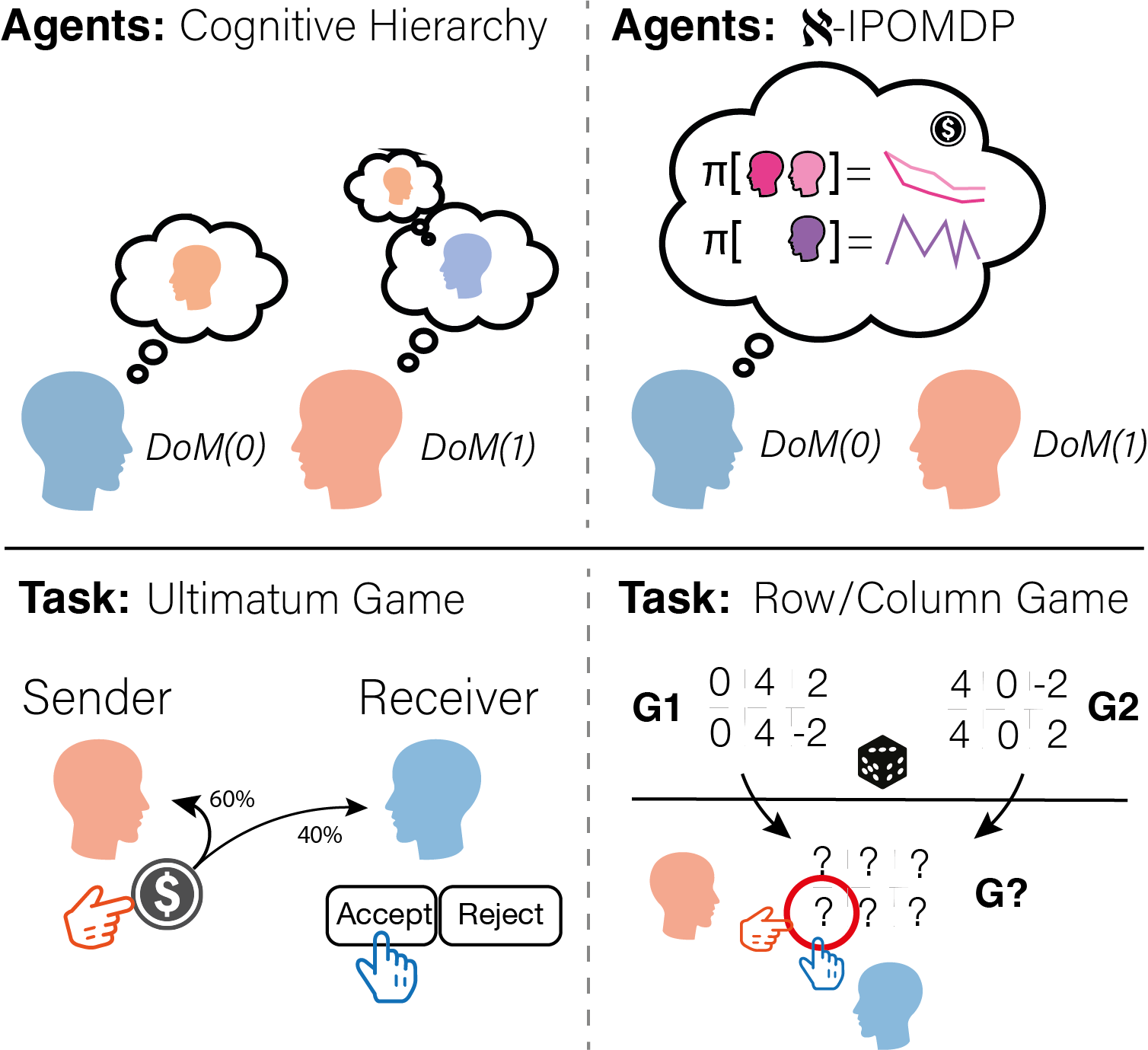
Figure 1: Paper overview: (Cognitive Hierarchy:) Agents with finite recursive opponent modeling with varying Depth of Mentalisation (DoM) interact in different environments. ($\aleph$-IPOMDP:) Augmenting agents’ inference processes with an anomaly detection mechanism allows them to cope with deceptive others. (IUG:) Agents with different degrees of DoM interact in the iterated ultimatum game (IUG). (Row/column game:) Agents interact in an iterated Bayesian zero-sum game, where deception takes place as well.

In this work, we present a computational framework for multi-agent RL (MARL) called $\aleph$-IPOMDP. We augment the well-known IPOMDP approach [Gmytrasiewicz and Doshi, 2005] to allow agents to engage with unmodeled opponents. We first discuss how agents use their ToM to manipulate others, preying on the limited computational resources of their victims. We then present the main contribution of this work: a deception detection mechanism, the $\aleph$-mechanism, by which agents with shallow DoM use a heuristic to detect that they are being deceived, and the OOB $\aleph$-policy, aimed at best-responding to the unknown opponent. We illustrate this mechanism in both mixed-motive and zero-sum Bayesian repeated games to show how $\aleph$-IPOMDP agents can mitigate the advantages of agents with deeper recursive models, and deter manipulation.

Our work is relevant to multiple fields. To the MARL community, our work serves to show how agents with limited opponent modeling (for example bounded rationality agents) can still cope with more adequate opponents via anomaly detection and game theoretic principles. To the cybersecurity community, we present a MARL masquerading detection use-case which can be used to overcome a learning adversarial attacks [Rosenberg et al., 2021]. To the psychology community, we provide a heuristic mechanism that may become maladaptively sensitive and overestimate deception, providing a model of suspicious or conspiratorial thinking. Lastly, there has recently been substantial interest in AI deception [Sarkadi et al., 2019b, 2021, Savas et al., 2022]. Our work may serve as a blueprint for systems that regulate and possibly prevent AI from deceiving other AI or humans.

2 Previous work

The recursive structure of ToM implies that it is impossible to make inferences about agents with DoM levels that are higher than one’s own. This is because modelling a more sophisticated agent would require one to model oneself—outside of the DoM hierarchy—and thus, at least in principle, to violate key logical principles [Pacuit and Roy, 2017]. Such a restriction is not unique to ToM-based models but is evident in general bounded rationality environments [Nachbar and Zame, 1996].

Methods of detecting masquerading using information theory have previously been used as a method for inferring deception in the context of intrusion detection. For example, Evans et al. [2007] used the MDLCompress algorithm to identify intruders disguised as legitimate users. Maguire et al. [2019] suggest that humans apply a typical set-like mechanism to identify a non-random pattern. However, this is very specific to random behaviour, while in this work we explore various deviations from expected behaviour. Behavioural based Intrusion Detection Systems (IDS) methods were proposed by Pannell and Ashman [2010], Peng et al. [2016]. In these systems, the system administrator monitors the behaviour of users to decide and respond to malevolent behaviour. However, unlike our proposed method, these systems often require labeled data making them susceptible to an aware adversary who knows how to avoid detection.

In the context of POMDP, several goal recognition methods have been proposed, for example: Ramırez and Geffner , Le Guillarme et al. [2016]. While these methods assume that the observed agent may be ill-intent they both assume that (a) the observer can invert the actions to infer about the goals, and (b) they both utilize the observed behaviour likelihood for intent recognition. In this work we show how likelihood based inference is used against the inferring agent as well as proposing a mechanism that detects deviation from expected behaviour, flagging out malevolent agents without the need to make inference about their goals.

Furthermore, Yu et al. [2021] explore how to adapt to higher DoM agents. They suggest that an agent can learn a best response against each $k$ level opponent from experience. However, it lacks the mechanism to detect when the opponent DoM level exceeds the agent’s DoM level and hence the agent should retrain its model.

3 Model

In this work, we propose a general framework, the $\aleph$-IPOMDP that augments the conventional IPOMDP framework (which involves recursive reasoning in an intentional POMDP) with a mechanism for detecting anomalous behaviour and an out-of-belief policy that serves as a deterrent. We first review these new components and then illustrate their effectiveness in deflecting deception in repeated Bayesian games.

Repeated Bayesian games model a series of interactions between agents with partial information. Agents may be uninformed about their state (e.g., the cards they are holding), the states of others (their cards) and social orientation (friend or foe), and so on. Agents address this uncertainty by forming beliefs about such unknown quantities, which they are then assumed to update in a Bayesian manner from observations. Each agent in these games is characterized by its type, ($\theta\in\Theta$) [Harsanyi, 1968]. The type describes all the parameters governing the agent’s decision-making—its utility ($u(\cdot)$) and beliefs ($b(\cdot)$), where these beliefs may include beliefs about the types (including the beliefs) of other agents. We index the inferring agent by $\alpha$ and their opponent by $\beta$.

Agents interact with each other by acting ($a_{\alpha}^{t}$) and observing others’ actions ($a_{\beta}^{t}$). The history, $h^{t}=\{a_{\alpha}^{0},a_{\beta}^{0},\cdots,a_{\alpha}^{t},a_{\beta}^{t}\}$, is a vector of actions that are used to make inferences about the opponent’s type and their state if that is also unobserved (which, for convenience, we avoid here):

$$b_{\alpha}^{t+1}(\theta_{\beta})=p(\theta_{\beta}|h^{t})\propto P(h^{t}|\theta_{\beta})p(\theta_{\beta})$$ (1)

In this work we do away with environmental uncertainty or include it as part of the opponent’s type for reduction of complexity.

We consider games in which agents form finitely recursive beliefs about others (known as cognitive hierarchy). At the basic level agents only maximize their utility based on whatever information they have at hand. These agents, known as subintentional or DoM$(-1)$ agents do not model their opponent at all, treating their opponent as part of the environment. DoM$(0)$ agents make inferences about the goals (utility) of DoM$(-1)$ ones, in a process similar to Bayesian-IRL [Ng and Russell, 2000, Ramachandran and Amir, 2007]:.

$$b_{\beta_{0}}^{t+1}(\theta_{\alpha})=$$ (2)

$$p(u_{\alpha_{-1}}(\cdot)|h^{t})\propto P(a_{\alpha}^{t}|u_{\alpha_{-1}}(\cdot),h^{t-1})p(u_{\alpha_{-1}}(\cdot)|h^{t-1})$$

Agents with higher DoM level (DoM$(k)$, $k\in[1\dots)$) also form beliefs about the beliefs of others, inferring others’ beliefs about them (“what do you think about me”) and so on:

$$b_{\alpha_{k}}^{t+1}(\theta_{\beta_{k-1}})=p(u_{\beta_{k-1}}(\cdot),b_{\beta_{k-1}}^{t}(\theta_{\alpha_{k-2}})|h^{t})$$ (3)

where $b_{\beta_{k-1}}^{t}(\theta_{\alpha_{k-2}})$ are the nested beliefs of others. The DoM$(k)$ agents use their beliefs to compute the action value:

$$Q(a_{\alpha}^{t};u_{\alpha},b^{t}_{\alpha_{k}}(\theta_{\beta_{k-1}}))=$$ (4)

$$E_{a_{\beta}^{t}\sim\hat{\pi}(\theta_{\beta})}[u_{\alpha}(a_{\alpha}^{t},a_{\beta}^{t})+\underset{a_{\alpha}^{t+1}}{\max}\{Q(a_{\alpha}^{t+1};u_{\alpha},b^{t+1}_{\alpha_{k}}(\theta_{\beta_{k-1}}))\}]$$

where $\hat{\pi}(\theta_{\beta})=\hat{\pi}(u_{\beta_{k-1}},\hat{b}_{\beta_{k-1}}(\theta_{\alpha_{k-2}}))$ is the simulated policy of a type $\theta_{\beta_{k-1}}$ opponent after observing $a^{t}_{\alpha}$, represented by $\hat{b}_{\beta_{k-1}}(\theta_{\alpha_{k-2}})$ (which are $\alpha$’s nested beliefs about $\beta$’s uncertainty about $\alpha$) Agents then select an action using a SoftMax policy with known inverse temperature $\mathcal{T}$:

$$P(a_{\alpha}^{t};\!u_{\alpha},\!b^{t}_{\alpha_{k}}(\theta_{\beta_{k-1}}))\!\propto\!\exp\!\textstyle\frac{1}{\mathcal{T}}Q(a_{\alpha}^{t};\!u_{\alpha},\!b^{t}_{\alpha_{k}}(\theta_{\beta_{k-1}}))$$ (5)

Since agents update their beliefs from observation, savvy opponents can shape the agent’s beliefs (and consequent behaviour) by choosing specific actions [e.g.  Alon et al., 2023b, a]. For example, in [Alon et al., 2023b], through judicious planning, buyers with higher DoM fake interest in an undesired item in a buyer-seller task. This is intended to deceive an observing seller into forming false beliefs about the buyer’s preferences, causing the seller to offer the buyer’s desired item at a lower price. These deceptive dynamics take advantage of two built-in features of recursive reasoning. One is the deceiver’s ability to simulate the victim’s reaction (at least up to epistemic uncertainty) :

$$P(a_{\beta}^{t}|a_{\alpha}^{t})\!=\!\sum_{\theta_{\beta}}P(a_{\beta}^{t}|\hat{\pi}(u_{\beta_{k-1}},\hat{b}_{\beta_{k-1}}(\theta_{\alpha_{k-2}}))b_{\alpha_{k}}^{t-1}(\theta_{\beta})$$ (6)

This allows the deceiver to affect the behaviour of a lower DoM victim to its benefit. It is similar to “white-box” adversarial attacks, when the attacker possesses the blueprints of its victim’s decision-making Ebrahimi et al. [2018]. Since the victim is limited to making inferences about lower-level DoM agents, they cannot directly interpret the deceiver’s actions as being deceptive. Violating this constraint would imply that the victim would be capable of self-reflection, violating logical principles [Pacuit and Roy, 2017]. The combination of the deceiver’s ability to deceive and the victim’s inability to resist deception spells doom for the lower DoM victim.

The central idea of this paper is that, despite these limitations in their opponent modelling, the victim may still realize that they lack the measure of their opponent, and thus can resist. The realization stems from assessing the (mis-)match between the expected (based on the victim’s lower DoM) and observed behaviour of the opponent—a form of heuristic behaviour verification. For example, consider a parasite, masquerading as an ant to infiltrate an ant colony and steal the food. While its appearance may mislead the guardian ants, its behaviour—feasting instead of working—should trigger an alarm. Thus, even if the victim lacks the cognitive power to resist manipulation, they can detect the ploy through a form of conduct validation.

If the victim detects such a discrepancy, it can conclude that the observed behaviour is generated by an opponent that lies outside their world model. In principle, there is a wealth of possibilities for mismatches, from the form of the DoM$(-1)$ or DoM$(0)$ agent to priors. Here, though, we assume that the only source of external types is the limited DoM level. Given the infinite number of DoM levels (bounded below by $(-1)$), of which only a finite subset lies within the $k$-level world-model ($\Theta_{k}\subset\Theta$), we denote this external set by $\Theta_{\aleph}$. For a DoM$(k)$ agent, all the possible DoM$(k-1)$ models are in $\Theta_{k}$. Thus, a mismatch between the observed and expected behaviour implies that the unknown agent has DoM level different than $(k-1)$. This is a pivotal concept, allowing the agent to engage with a known, yet unmodeled, opponent.

Once the behavioural mismatch has been identified, the victim has to decide how to act. Defensive counter-deceptive behaviour should take into account the observation that an out-of-model deceiver might have the capacity to predict the victim. Thus, the victim’s policy could be aimed at hurting the deceiver (at a cost to the victim), to deter them from doing so.

3.1 Detecting and responding to deception with limited opponent model

Detecting abnormal, and potentially risky, behaviour from observed data is related to Intrusion Detection Systems (IDS). This domain assumes that “behaviour is not something that can be easily stole[n]” [Salem et al., 2008]. Thus, any atypical behaviour is flagged as a potential intruder, alarming the system that the observed user poses a risk to the system.

Several methods have been suggested to combat a masquerading hacker [Salem et al., 2008]. Inspired by these methods, we augment the victim’s inference with what we call an $\aleph$-mechanism. This mechanism, $f(\Theta_{k},h^{t})$, evaluates the opponent’s behaviour against the expected behaviour, based on the agent’s DoM level and the history. The expected behaviour includes the presumed opponent’s response to the agent’s actions, in a way similar to the simulated policy in Equation 6. The $\aleph$-mechanism returns a binary vector of size $|\Theta_{k}|$ as an output. Each entry represents the $\aleph$-mechanism’s evaluation per opponent type: $\theta_{\beta}\in\Theta_{k}$. The evaluation either affirms or denies that the observed behaviour (discussed next) sufficiently matches the expected behaviour of each agent type.

A critical issue is that, as in Liebald et al. [2007], we allow the deceiver to be aware of the detailed workings of the $\aleph$-mechanism, and so be able to avoid detection by adhering to the regularities underlying it. This renders many methods impotent for detecting deception. Nonetheless, two key factors of deception make it detectable. First, to execute its deception, the deceiver will have to deviate from the typical behaviour of the masqueraded agent at some point. For example, a hacker masquerading as a legitimate user will try at some point to access sensitive data—a non-typical behaviour for the benevolent user. This alerts the victim that they might be engaging with an unmodeled agent. Second, in non-cooperative games, the deceiver’s reward maximization is at the expense of the victim. Since the victim uses their ToM to compute the expected cumulative reward (from Equation 4), then if the actual reward deviates (statistically) from the expected reward, it is another indication that the opponent is not in the world model of the victim.

3.1.1 $\aleph$-mechanism

The behaviour verification mechanism assesses whether the observed opponent belongs to the set of potential opponents using two main concepts: $\delta$-strong typical set and expected reward. The $\delta$-strong typical set is an Information Theory (IT) concept, defined as the set of realizations from a generative model with empirical and theoretical frequencies that are sufficiently close according to an appropriate measure of proximity. If an observed trajectory does not belong to this set there is a high probability that it was not generated by the underlying opponent model. The second component confirms that the reward is consistent with the expected reward (averaged across types).

Formally, let $\hat{F}_{h^{t}}(a^{\prime}_{\beta})$ denote the empirical likelihood of an opponent action, defined as $\hat{F}_{h^{t}}(a^{\prime}_{\beta})=\nicefrac{{N(a^{\prime}_{\beta})}}{{|h^{t}|}}$, where $N(a^{\prime}_{\beta})$ is the number of times the action $a^{\prime}_{\beta}$ appears in the history set. The $\delta$-strongly typical set of the trajectories, for agent with type $\theta$, is the set:

$$T_{\delta}(\theta_{\beta})=\{h^{t}:|\hat{F}_{h^{t}}(a^{\prime}_{\beta})-F_{\theta_{\beta}}(a^{\prime}_{\beta})|\leq\delta\cdot F_{\theta_{\beta}}(a^{\prime}_{\beta})\}$$ (7)

where $F_{\theta_{\beta}}(a^{\prime}_{\beta})$ is the theoretical probability that an agent with type $\theta_{\beta}$ will act $a^{\prime}_{\beta}$ across rounds. This component of the $\aleph$-mechanism, denoted by $g_{1}(\Theta_{k},h^{t},\delta)$, outputs a binary vector. Each entry in the vector indicates whether or not the observed sequence belongs to the $\delta$-strong typical set of $\theta_{\beta}\in\Theta_{k}$.

The parameter $\delta$ governs the size of the set, which in turn affects the sensitivity of the mechanism. It can be tuned using the nested opponent models to reduce false positives. However, since the deceiving agent model is absent from this “training” set, this parameter cannot be tuned to balance true negatives. An additional issue with setting this parameter is its lack of sensitivity to history length. This poses a problem since the empirical frequency is a function of the sample size. We address this issue by making trial-dependent, denoted by $\delta(t)$. We discuss task-specific details in Appendix 6.1.2.

The second component, denoted by $g_{2}(\Theta_{k},h^{t},r^{t},\omega)$, verifies the opponent type by comparing the expected reward to the observed reward. In any MARL task, agents are motivated to maximize their utility. In mixed-motive and zero-sum games, the deceiving agent increases its portion of the joint reward by reducing the victim’s reward. This behaviour will contradict the victim’s expectations to earn more (due to it assumption that it has the higher DoM level). Hence, it is expected that the victim is as sensitive to deviation from the expected reward as to other sorts of abnormal behaviour (such as those picked up by the $\delta$-strong typicality component). Due to the coupling between the agent’s reward and its actions, this component computes the history-conditioned expected reward $\hat{r}_{\alpha}^{t}$, by averaging the expected actions and reactions per type. Formally, the expected reward, per opponent type is:

$$\hat{r}_{\alpha}^{t}(\theta_{\beta_{k-1}})=E_{a_{\alpha}^{t}\sim\pi_{\alpha}}[E_{a_{\beta}^{t}\sim\hat{\pi}_{\beta}}(u_{\alpha}(a_{\alpha}^{t},a_{\beta}^{t}))|h^{t-1}]$$ (8)

Accounting for the random behaviour stemming from the presumed SoftMax policy, the empirical reward is verified to be within an $\omega$ confidence interval: $r_{\alpha}^{t}\in[\hat{r}_{\alpha}^{t}\pm z_{\omega}\sigma(\hat{r}^{t})]$, where $\sigma(\hat{r}_{\alpha}^{t})$ is the standard deviation of the reward (which has similar dependencies as in equation 8). This component’s output is similar to the output of $g_{1}(\Theta_{k},h^{t})$, namely a vector of size $|\Theta_{k}|$ with each entry is a binary variable, indicating if the observed reward is within the CI or not, implying whether the reward is generated by a $\theta_{\beta}\in\Theta_{k}$ opponent. Notably, if the expected reward is higher than the upper limit this component is activated, even though such an event benefits the victim. This component may be tuned to only alert when the expected reward is too low, however, this modification doesn’t affect the detection as we assume that the deception is aimed at harming the victim.

The output of both components is combined using logical conjunction: $f=g_{1}(\cdot)\wedge g_{2}(\cdot)$. Notably, the components are correlated, as $\alpha$’s reward , monitored by $g_{2}$ is a function of $\beta$’s actions, which are monitored by $g_{1}$. The mechanism is described in Algorithm 1. The output, a binary vector, is then taken as input by the $\aleph$-policy alongside the beliefs.

Algorithm 1 $\aleph$-mechanism

Input: $\Theta_{k},h^{t},r^{t},\delta,\omega$
      Output: $f$

1:procedure $\aleph$-Mechanism($\Theta_{k},h^{t},r^{t},\delta,\omega$)

2:     $x\leftarrow g_{1}(\Theta_{k},h^{t},\delta)$

3:     $y\leftarrow g_{2}(\Theta_{k},h^{t},r^{t},\omega)$

4:     $f\leftarrow x\wedge y$

5:     return $f$

6:end procedure

7:procedure $g_{1}$($\Theta_{k},h^{t},\delta$)

8:     Compute $T_{\delta}(\theta)$ $\triangleright$ From 7

9:     $x\leftarrow h^{t}\in T_{\delta}(\theta)$

10:     return $x$

11:end procedure

12:procedure $g_{2}$($\Theta_{k},h^{t},r^{t},\omega$)

13:     Compute $\hat{r}^{t}$ given $h^{t}$ $\triangleright$ From 8

14:     $y\leftarrow r^{t}\in[\hat{r}^{t}\pm z_{\alpha}\sigma(\hat{r}^{t})]$

15:     return $y$

16:end procedure

3.1.2 $\aleph$-policy

The agent’s behaviour is governed by its $\aleph$-policy (Algorithm 2). It takes as an input the output of the $\aleph$-mechanism and the updated beliefs. If the opponent’s behaviour passes the $\aleph$-mechanism, the agent behaviour is its DoM$(k)$ policy, in this work a SoftMax policy. Here we use the IPOMCP algorithm for the Q-values computation Hula et al. [2015]. This algorithm extends the POMCP algorithm for IPOMDP, however any planning algorithm is applicable. In the case that the opponent’s behaviour triggers the $\aleph$-mechanism, the victim’s optimal policy switches to an OOB policy. While lacking the capacity to simulate the external opponent, the $\aleph$-policy utilizes the property highlighted above: the victim knows that the deceiver is of an unknown DoM level. If the deceiver’s DoM level is higher than the victim’s, it means that the deceiver can fully simulate the victim’s behaviour. Hence, if the OOB policy derails the opponent’s utility maximization plans, the opponent will avoid it. The best response inevitably depends on the nature of the task. We illustrate the $\aleph$-IPOMDP for two different payout structures: zero-sum and mixed-motive.

In zero-sum games, the Minimax algorithm [Shannon, 1993] computes the best response in the presence of an unknown opponent. This principle assumes that the unknown opponent will try to act in the most harmful manner, and the agent should be defensive to avoid exploitation. While this policy is beneficial in zero-sum games it is not rational in mixed-motive games; it prevents the agent from taking advantage of the mutual dependency of the reward structure.

In repeated mixed-motive games Grim trigger [Friedman, 1971] and Tit-for-Tat [Milgrom, 1984, Nowak and Sigmund, 1992] policies have been suggested as ways of deterring a deceptive opponent. An agent following the Grim trigger policy responds to any deviation from cooperative behaviour with endless anti-cooperative behaviour, even at the risk of self-harm. While being efficient at deterring the opponent from defecting, this policy has its pitfalls. First, it might be that the opponent’s defective behaviour is by accident and random (i.e., due to SoftMax policy) and so endless retaliation is misplaced. Second, if both players can communicate, then a warning shot is a sufficient signal, allowing the opponent to change their nasty behaviour. This requires a different model, for example, the Communicative-IPOMDP [Gmytrasiewicz and Adhikari, 2019]. However, in this work, we illustrate how the presence of a simple Grim trigger policy suffices to deter a savvy opponent from engaging in deceptive behaviour.

Algorithm 2 $\aleph$-policy

Input: $b^{t}_{\alpha_{k}}(\theta_{\beta_{k-1}}),f$
      Output: $a^{t+1}$

1:procedure $\aleph$-Policy($b^{t}_{\alpha_{k}}(\theta_{\beta_{k-1}}),f$)

2:     if $f\neq 0$ then:

3:         $a^{t+1}\sim\pi(b^{t}_{\alpha_{k}}(\theta_{\beta_{k-1}}))$

4:     else 

5:         $a^{t+1}$ is sampled from OOB policy

6:     end if

7:     return $a^{t+1}$

8:end procedure

4 Applications in repeated Bayesian games

To illustrate the effectiveness of the $\aleph$-IPOMDP in mitigating manipulation in repeated Bayesian games, we compare it to unadorned $k$-level reasoning (IPOMDP) in a mixed-motive and a zero-sum game. The IPOMDP serves as a baseline to the $\aleph$-IPOMDP models. This comparison shows how the ability to detect and resent deception improves the lower DoM agent’s outcome by serving as a protection mechanism, limiting the higher DoM agent’s deceptive strategies. In both games, the $\aleph$-IPOMDP can reduce the reward gap between the deceiver and victim compared to the IPOMDP case.

4.1 Mixed-motive game

The iterated ultimatum game (IUG) [Camerer, 2011, Alon et al., 2023a] (illustrated in Fig 1(Ultimatum Game); described in detail inAlon et al. [2023a]) is a paradigmatic repeated Bayesian mixed-motive game. Briefly, the game is played between two agents—a sender ($\alpha$) and a receiver ($\beta$). On each trial of the game, the sender gets an endowment of 1 monetary unit and offers a partition of this sum to the receiver: $a^{t}_{\alpha}\in[0,1],t\in[1,T]$. If the receiver accepts the offer $(a^{t}_{\beta}=1)$, the receiver gets a reward of $r^{t}_{\beta}=a^{t}_{\alpha}$ and the sender a reward of $r^{t}_{\alpha}=1-a^{t}_{\alpha}$. Alternatively, the receiver can reject the offer $(a^{t}_{\beta}=0)$, in which case both parties receive nothing. In this game, agents need to compromise (or at least consider the desires of the other), but at the same time wish to maximise their reward—making the task a useful testbed for the advantages of high DoM.

We simulated senders with 2 levels of DoM: $k\in[-1,1]$ interacting with a DoM$(0)$ receiver, in addition, we include a uniformly random sender. All non random agents select actions via a SoftMax policy (Eq. 5) with known temperature ($\mathcal{T}=0.1$) . Each non-random sender is also characterized by a threshold, $\eta\in\{0.1,0.5\}$, which is a parameter of its subjective utility: $u^{t}_{\alpha}(a^{t}_{\alpha},a^{t}_{\beta},\theta_{\alpha})=(1-a^{t}_{\alpha}-\eta_{\alpha})\cdot a^{t}_{\beta}$.

Each agent uses its nested model of the opponent for inverse inference and planning. The DoM$(0)$ receiver infers from the offers about the type of the DoM$(-1)$ sender—random or threshold using an IRL process (Eq. 2). It then integrates these beliefs into its Q-value computation (via Expectimax search [Russell, 2010]). The DoM$(1)$ sender simulates the DoM$(0)$ receiver’s beliefs and resulting actions during the computation of its Q-values using the IPOMCP algorithm [Hula et al., 2015].

As hypothesized, in the pure IPOMDP case, agents with high DoM levels take advantage of those with lower DoM levels. The complexity of this manipulation rises with the agents’ cognitive hierarchy. The DoM$(0)$ receiver infers the type of the DoM$(-1)$ sender and uses its actions to alter the behaviour of the sender (if possible). Specifically, it tricks the threshold DoM$(-1)$ sender to offer more via strategic rejection (as illustrated in Fig. 5). On the other, since the random sender affords no agency, the optimal policy for the receiver, in this case, is to accept any offer.

This behaviour drives the DoM$(1)$ sender’s ploy. It hacks the DoM$(0)$ IRL using its DoM$(0)$ nested model. Its policy causes the DoM$(0)$ to falsely believe that it engages with a random agent, by sending a relatively high first offer, as illustrated in Fig. 2(A). It then executes its ruse by reducing offers and exploiting the DoM$(0)$ receiver’s docile behaviour against what this receiver falsely perceives to be a random sender (Fig. 2(B)). A full analysis of this is presented in Alon et al. [2023a] and in Appendix 6.1. This ploy yields the DoM$(1)$ sender a considerable higher cumulative reward compared to the DoM$(0)$ receiver (Fig. 3(B)).

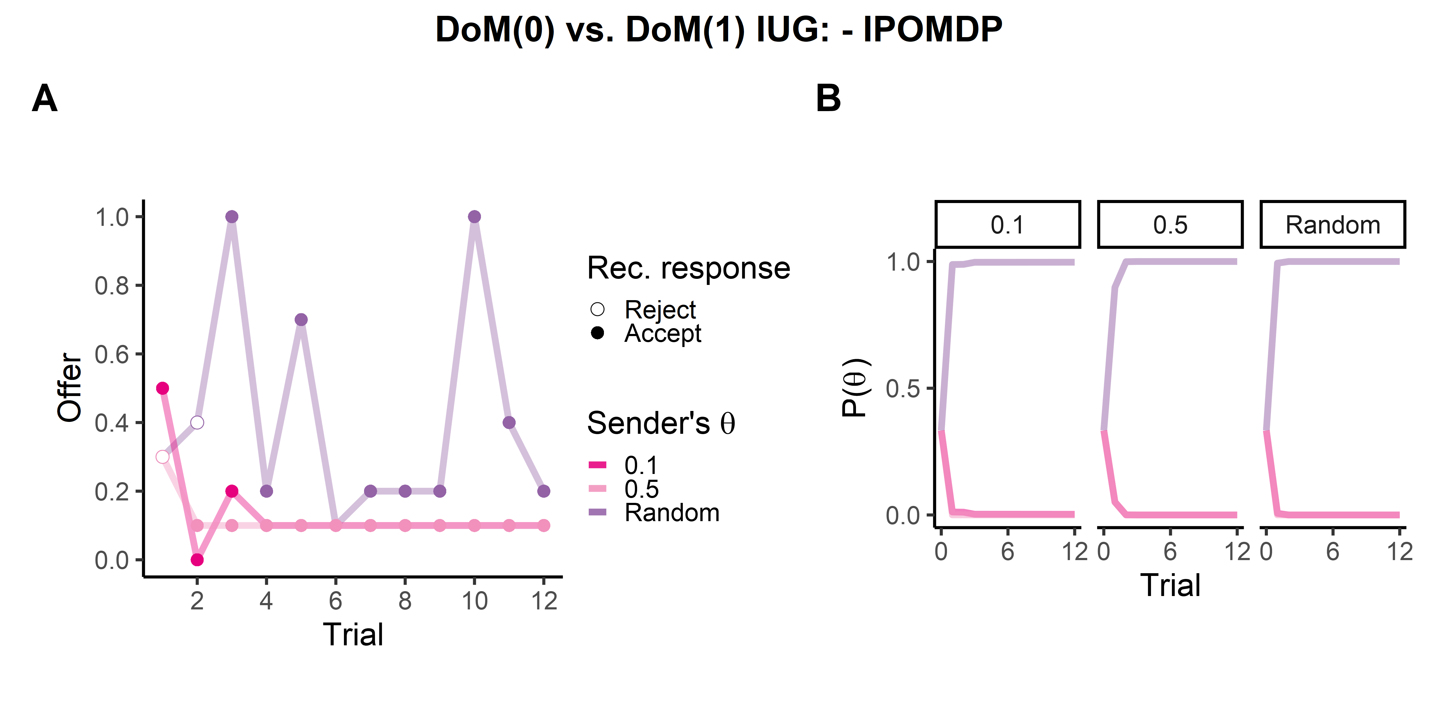
Figure 2: Illustration of deception in IUG: (A) The DoM$(1)$ acts in a deceptive way to masquerade itself as a random sender, hacking the DoM$(0)$ Bayesian IRL, starting with a relatively high first offer, before sharp decrease. (B) This stratagem exploits the pitfall of Bayesian inference—the likelihood that any offer sequence is equal for the random sender.

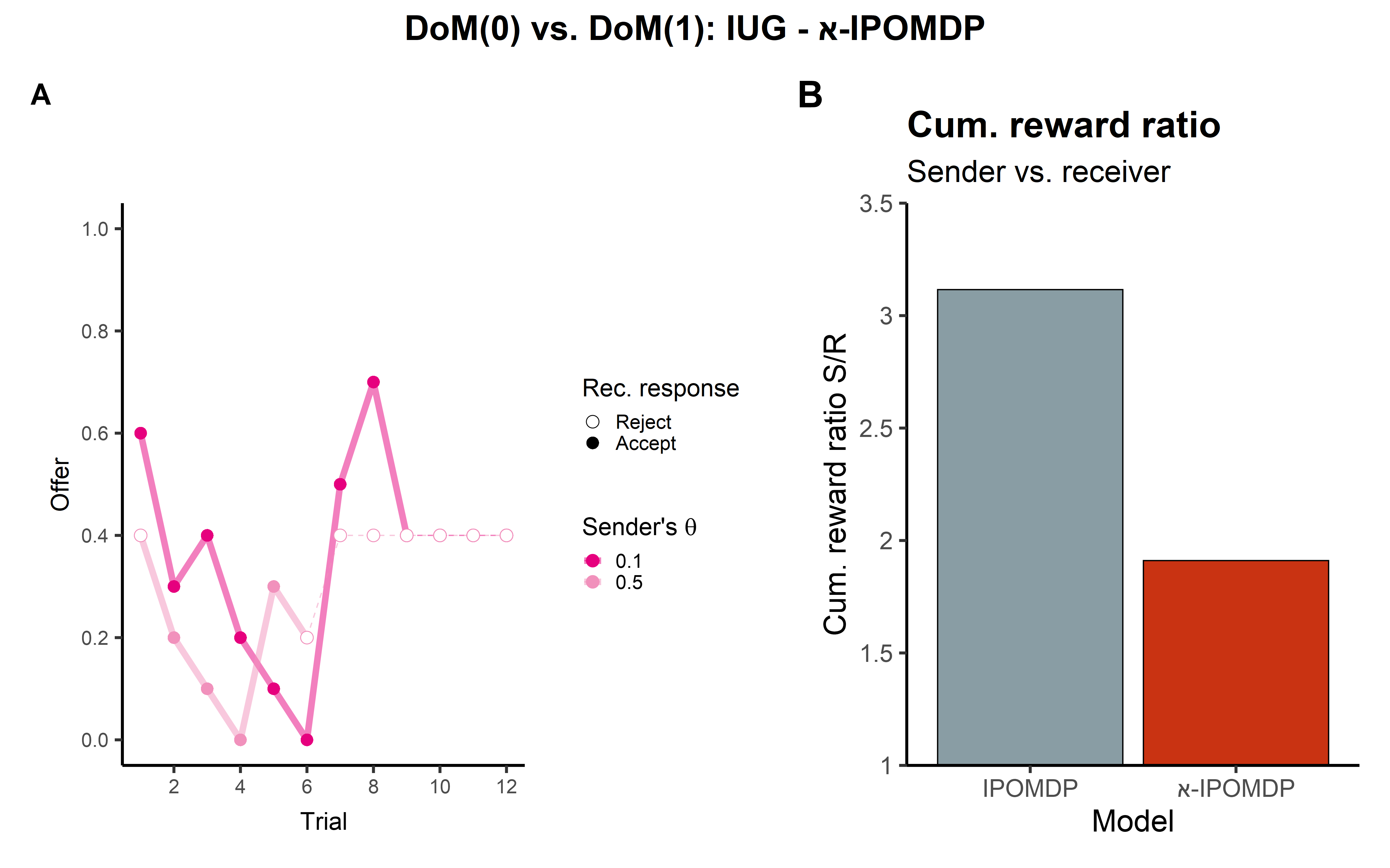
Figure 3: Mitigation of deception in IGU with $\aleph$-IPOMDP: (A) Trapped by the $\aleph$-mechanism’s typical set and expected reward monitoring, the DoM$(1)$ sender cannot execute its deception. Instead, the DoM$(1)$ is forced to apply a different strategy, offering higher offers to the receiver until it is bounded by its utility. (B) In turn, this reduces the cumulative reward ratio (sender/receiver) by more than $40\%$.

Repeating the simulation with the $\aleph$-IPOMDP framework allows us to illustrate how this power structure is diluted via the detection and retaliation of the $\aleph$-mechanism and $\aleph$-policy. The parameter tuning is detailed in Appendix 6.1.2. As mentioned above, the $\aleph$-policy is the Grim Trigger policy. The effect of the $\aleph$-IPOMDP is illustrated in Fig. 3. First the $\aleph$-mechanism and the $\aleph$-policy change the deceiver’s behaviour (compare Figures 2(A) and 3(A)). Each component limits the deceiver’s actions if it wishes to avoid detection. Masquerading again as a random sender, the deceiver has to adhere to the statistical regularities of the $\aleph$-mechanism. This is illustrated by the varying offers sequence, avoiding repeating the same offer twice until the “desirable” offer set (as defined by the sender’s type) is depleted, after which the sender deliberately triggers the $\aleph$-mechanism, effectively terminating the interaction as marked by the line-type. In turn, this limitation reduces the income gap between the agents, as illustrated in Fig. 3)(B). The size of the inequality reduction is a function of the $\aleph$-mechanism parameters. Narrow the expected reward bounds, by setting small $\omega$, will force the deceiver to make offers that are closer to the masqueraded agent mean offers, reducing the size of the set of available actions (to avoid alerting the victim). Setting larger values of $\delta$ allows the deceiver to repeat the offer several times. The combination of the two determines the outcome of the game. However, this rigidity may harm the victim’s performance when interacting with a genuine random agent, in the case of the IUG task. Hence, setting these parameters requires a delicate balancing of false and true negatives with some desired reward metric.

4.2 A Zero-sum game

Deception is not limited to mixed-motive games, it may also occur in zero-sum games. A canonical example is Poker [Palomäki et al., 2016], where players deliberately bluff to lure others into increasing the stakes, only to learn in hindsight that they were tricked. Simple such games were presented and solved by [Zamir, 1992]. Here, we present an RL variant of one of these games [Example 1.3; Zamir, 1992], modeling it with ToM, illustrating how the $\aleph$-IPOMDP allow the bestowed victim to resist the manipulation.

Two agents with different DoM levels play the game presented in Fig. 1(Row/Column game). In this game, one of two payout matrices $G_{1},G_{2}$ (Eq. 9) is picked by nature with equal probability, the entries denote the row player payoff.

$$G^{1}=\begin{pmatrix}4&0&2\\ 4&0&-2\end{pmatrix},G^{2}=\begin{pmatrix}0&4&-2\\ 0&4&2\end{pmatrix}$$ (9)

The row player $(\alpha)$ may or may not know which matrix is selected (also with equal probabilities), while the column player $(\beta)$ is always ignorant of this outcome. We denote by $\theta_{\alpha}\in\{0,1,2\}$ the row player’s type, where $1,2$ mark that $\alpha$ knows which payoff matrix is sampled. For $T>0$ trials the agents simultaneously choose actions. The row player picks either the Top or Bottom row, while the column player selects the Left, Middle or Right column. The payoff is according to the selected cell. Crucially, the agents get the cumulative reward only at the end of the game and do not get an intermediate reward throughout. This limits $\beta$’s inference to depend only on $\alpha$’s actions. Each agent selects its actions to maximize its discounted long-term reward. Agents compute Q-values using their DoM level and the history, and select an action via SoftMax (Eq.5) policy with a known $\mathcal{T}$. A detailed description of the game is presented in Appendix 6.2.

The informed DoM$(-1)$ row player ($\theta_{\alpha_{-1}}\in\{1,2\}$) assumes a uniform column player $Q_{\alpha_{-1}}(a_{\alpha}|\theta_{\alpha_{-1}})=E_{a_{\beta}\sim U}[u_{\alpha}(a_{\alpha},a_{\beta})]$. The DoM$(0)$ column player makes inference about the payoff matrix from the DoM$(-1)$ actions (Eq. 2). For example, if the row player constantly plays $T$, this is a strong signal that the payoff matrix is $G_{1}$, as this action’s q-value is $Q_{\alpha_{-1}}(T|\theta_{\alpha_{-1}}=1)=2$ compared to $Q_{\alpha_{-1}}(B|\theta_{\alpha_{-1}}=1)=\nicefrac{{2}}{{3}}$. Using these beliefs it computes the Q-value of each action:

$$Q_{\beta_{0}}(a_{\beta}|b_{\beta_{0}}(\theta_{\alpha_{-1}}))=E_{a_{\alpha}\sim\pi_{\alpha_{-1}}(\theta_{\alpha_{-1}})}[u_{\beta}(a_{\alpha},a_{\beta})]$$ (10)

Its policy is to select the column that yields it and the row player a $0$ reward ($L$ in $G_{1}$ and $M$ in $G_{2}$). In turn, DoM$(1)$ row player tricks the DoM$(0)$ into falsely believing that the payoff matrix is the other one (for example, if the true payout matrix is $G_{1}$ it acts in a way typical for a DoM$(-1)$ in $G_{2}$). This deception utilizes the same concepts as in the IUG—the limited opponent modeling of the lower DoM column player and its Bayesian IRL (illustrated in Fig. 4(A)-left column). In turn, the DoM$(0)$ Q-values computation (Eq. 10) takes as input these false beliefs, resulting in selection of the column that instead of yielding it a $0$ reward, is actually the least favourable column ($M$ in $G_{1}$, $L$ in $G_{2}$) yielding it a negative utility of $-4$. This substantially benefits the DoM$(1)$ row player. Using its nested DoM$(1)$ model, the DoM$(2)$ column player “calls the bluff” and makes correct inferences about the payout matrix Fig.(4(A). Its policy exploits the DoM$(1)$ ruse against itself as illustrated in Fig. 4(B), by picking the right column, yielding it a reward of $2$ and a reward of $-2$ to $\alpha_{1}$.

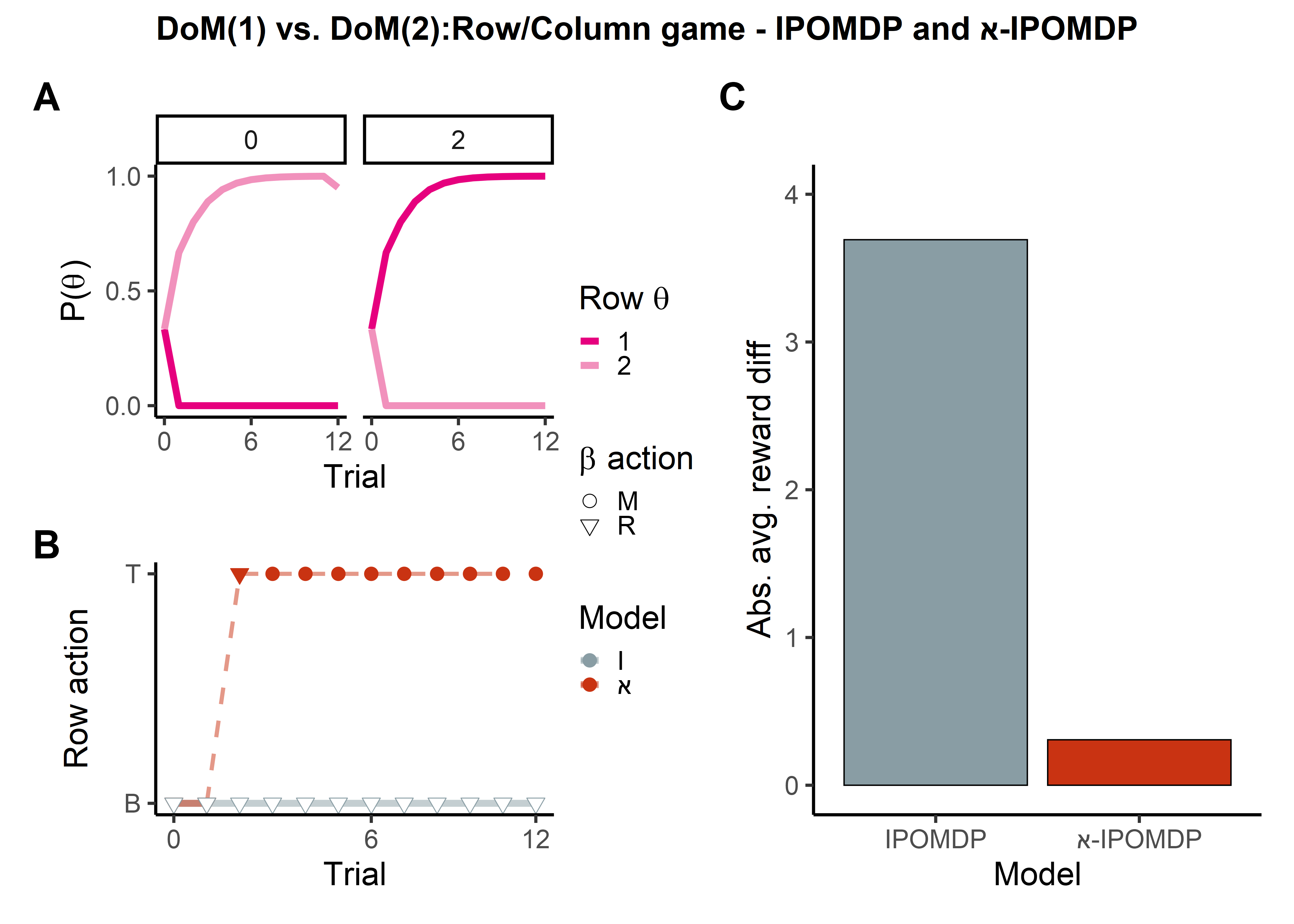
Figure 4: Effect of $\aleph$-IPOMDP in a zero sum game: (A) Interacting with a $\theta_{\alpha}=1$, the DoM$(0)$ (left column) is deceived by $\alpha$’s actions and form false beliefs. However, the DoM$(2)$ utilizes its nested model to read through the bluff and correctly identifies $\alpha$’s type. (B)(grey line) In turn, the DoM$(2)$ policy exploits of the DoM$(1)$ ruse against it. Augmented with $\aleph$-IPOMDP (red line), the DoM$(1)$ infers this unexpected behaviour as a sign of an external entity, triggering the $\aleph$-mechanism, marked by the dashed line. Its $\aleph$-policy causes the DoM$(2)$ column player to adapt and alter its abusive behaviour. (C) The effect of the $\aleph$-IPOMDP in this task is illustrated via the reduction in the average absolute reward difference.

Lacking the capacity to model such counter-deceptive behaviour, the DoM$(1)$ erroneously attributing this behaviour to the SoftMax policy, and its nested beliefs about the column player beliefs are the distorted DoM$(0)$ beliefs. This inability to resist manipulation by higher DoM column player yields high income gap, as illustrated in Fig.4(C). Simulating the task with the $\aleph$-IPOMDP framework solves this cognitive advantage asymmetry: the DoM$(1)$ detects the mismatch between its world model and its opponent, as the behaviour of the DoM$(2)$ is highly non typical for a $\beta_{0}$, triggering the $\aleph$-mechanism. The DoM$(1)$ MinMax $\aleph$-policy, i.e., playing truthfully, causes the DoM$(2)$ to adapt its behaviour appropriately (Fig. 4(B)). In this case, both parties get $0$ reward, which drops the average absolute reward difference compared to the IPOMDP case, as illustrated in Fig. 4(C).

5 Discussion

We imbued agents with the ability to assess whether they are being deceived, without (at least fully) having to conceptualise how. We do so by augmenting their Bayesian inference with the $\aleph$-IPOMDP mechanism, involving environmental and behavioural heuristic statistical inference. The $\aleph$-policy of these agents is based on a computational concept, the ability to infer that they are facing an agent outside of their world model that threatens to harm them. The net result is a more equitable outcome. This framework offers some protection to model-based IPOMDP agents that are at risk of being outclassed by their opponents.

We tested this mechanism in mixed-motive and zero-sum Bayesian repeated games. We show that our mechanism can protect the victim against a greedy, clever deceiver who utilizes its nested victim model to coerce the victim to act in a self-harming manner. Such a pretence depends on atypical sequences of actions detectable by the $\aleph$-mechanism. Of course, as in Goodhart’s law (“any observed statistical regularity will tend to collapse once pressure is placed upon it for control purposes”), the higher DoM agent can, at least if well-calibrated with its simpler partner, predict exactly when the $\aleph$-mechanism will fire, and take tailored offensive measures. However, the net effect in both games shows that their hands might be sufficiently tied to make the outcome fairer.

The two defining points for the $\aleph$-IPOMDP framework are the augmented inference (the $\aleph$-mechanism), and the policy computation (the $\aleph$-policy). For the inference, there could be, as we present here, exquisitely tailored parameters that perform most competently in a given interaction; however, this might not scale. One inspiration for the policy was the notion of irritation in the context of the multi-round trust task [Hula et al., 2018]. In terms of the $\aleph$-policy, total non-cooperation is a rather blunt, and often self-destructive, instrument—despite being a credible and thus effective threat [McNamara and Houston, 2002]. Alternatively, agents might decide that it is worth investing more cognitive effort, and then increase one’s DoM [Yu et al., 2021]. This could become a cognitively expensive arms race [Sarkadi, 2023].

Our model lacks the capacity to reason about the goals and plans of the deceiver, which may be crucial to facilitate opponent learning (as in the work of [Yu et al., 2021], where agents can learn how to adapt their recursive level via learning). A DoM$(k)$ agent would benefit from such an ability (say via self-play) in repeated interactions. However, a savvy opponent, aware of this learning capacity, can still manipulate the learning process to its benefit [Foerster et al., 2018]. Here, we show how to overcome this issue with limited, fixed computational capacity.

A particular concern for the $\aleph$-IPOMDP arises when the mismatch stems not from strategic manipulation but from simple model error or a discrepancy between the actual and assumed prior distributions over components of the opponent. This issue gives rise to two related problems. First, with the spirit of the no free lunch theorem, the parameters of the $\aleph$-policy need to balance sensitivity and specificity. The mechanisms might reduce false alarms at the expense of missing true deception, or might be overactive and cause the victim to misclassify truly random behaviour. The latter may result in paranoid-like behaviour Alon et al. [2023a]. Second, the model currently assumes k-level reasoning. This means that the $\aleph$-mechanism is activated by agents with lower than $k-1$ DoM level. However, a DoM$(k)$ is fully capable of modeling these agents, as they are part of its nested opponent models. Thus, following the ideas suggested by [Camerer et al., 2004], future work may extend the opponent set to include all DoM level up to $k$.

Opponent verification is relevant to cybersecurity [Obaidat et al., 2019], where legitimate users need to be verified and malevolent ones blocked. However, savvy hackers learn to avoid certain anomalies while still exploiting the randomness of human behaviour. To balance effectively between defence and freedom of use, these systems need to probe the user actively to confirm the user’s identity. Our model proposes one such solution, but lacks the active learning component, which future work may incorporate.

In keeping with its roots in competitive economics, we focused on how lower DoM agents might be exploited. One could also imagine the case that the higher DoM agent exceeds expectations by sharing more than the lower DoM agent expects. Although the lower DoM agent might consider this to be a ploy, it could also be a sign that the higher DoM has a social orientation ‘baked’ into its policy to a greater extent than expected. In this case, the lower DoM agent might want to have the capacity to compensate for the over-fair actions—perhaps an analogue of certain governmental subsidies. Naturally, these mechanisms are prone to excess manipulation, and so would need careful monitoring.

6 Appendix

6.1 Detailed description of the IUG task

The IUG task is presented in detail in Alon et al. [2023a]. Here we represent the game structure and the main dynamics for context. Let $\mathcal{O}$ denote the set of potential offers ($\alpha$’s actions), $a_{\alpha}\in[0,1]$ discretized in this work to bins of $0.1$, yielding 11 potential offers in total. In addition we set $T=12$ in this work. We model this interaction as an IPOMDP problem. The agents’ goal is to maximize their discounted cumulative reward $\sum_{t=1}^{T}e^{\Gamma t}u^{t}$, where $\gamma=\exp(\Gamma)\in[0,1]$ is a discount factor (here set to 0.99). Each agent computes the Q-values for its actions given the current history, its type and DoM level, for example, the Q-value of a DoM$(k)$ sender are denoted by: $Q_{\alpha_{k}}(a_{\alpha}^{t};h^{t-1},\theta_{\alpha})$.

The random sender’s actions are drawn uniformly, and do not react to the receiver’s responses. The threshold senders are characterized by both their threshold and their DoM level. This value is analogous to a seller’s wholesale price: if the reward is lower than $\eta_{\alpha}$, the utility is negative, and hence the action is unfavorable. In this problem, we follow the alternating cognitive hierarchy formation suggested by Hula et al. [2015], and first outline the respective senders and receivers.

The DoM$(-1)$ sender’s policy is simple and model-free—if the current offer is rejected, they offer more (up to their threshold) because rejection signals their offer was too low. In turn, if the offer is accepted, the DoM$(-1)$ sender offers less. Formally, these agents maintain two bounds that are updated online (and thus are a deterministic function of the history $h^{t-1}$):

$$L^{t} =L^{t-1}\cdot a^{t-1}_{\beta}+a^{t-1}_{\alpha}\cdot(1-a^{t-1}_{\beta})$$ (11)

$$U^{t} =U^{t-1}\cdot(1-a^{t-1}_{\beta})+a^{t-1}_{\alpha}\cdot a^{t-1}_{\beta}$$ (12)

with $L^{1}=0,U^{1}=1$. We make the further assumption that the agents are myopic, meaning that their planning horizon is limited to the current trial. Then, their Q-values are:

$$Q_{\alpha_{-1}}(a_{\alpha}^{t};h^{t-1},\theta_{\alpha}) =u^{t}_{\alpha}(a_{\alpha}^{t},\theta_{\alpha})*\mathds{1}_{a_{\alpha}^{t}\in(L^{t},U^{t}]}$$ (13)

where $\mathds{1}_{a_{\alpha}^{t}\in(L^{t},U^{t}]}$ is the indicator function, which equals $1$ if the offer is between the bounds. That is, it only computes the Q-values for actions in this set.

The DoM$(0)$ receiver models the sender as DoM$(-1)$. Since these agents do not form beliefs, the inference is limited to type inference, threshold: ($\theta_{\alpha_{-1}}=\eta_{\alpha})$ or random. The DoM$(0)$ receiver beliefs follow the general inverse reinforcement learning outlined in Equation 1:

$$b^{t}_{\beta_{0}}(\theta_{\alpha_{-1}})=$$ (14)

$$p^{t}(\eta_{\alpha}|h^{t-1},a_{\alpha}^{t})\propto P^{t}_{\alpha_{-1}}(a_{\alpha}^{t}|\eta_{\alpha},h^{t-1})p^{t-1}(\eta_{\alpha})$$

where $P^{t}_{\alpha_{-1}}(a_{\alpha}^{t}|\eta_{\alpha},h^{t-1})$ is computed from Equations 13 and 5 using bounds $L^{t},U^{t}$ that are, as noted, a deterministic function of the prior $h^{t-1}$. The Q-values of each action are:

$$Q_{\beta_{0}}(a_{\beta}^{t};a^{t}_{\alpha},h^{t-1},\theta_{\beta})=E_{a^{t+1}_{\alpha_{-1}}\sim\pi^{*}_{\alpha_{-1}}}\big{[}u^{t}_{\beta_{0}}(a^{t}_{\alpha},a_{\beta}^{t})+$$

$$\qquad\gamma\max\nolimits_{a^{t+1}_{R}}\{Q_{\beta_{0}}(a_{\beta}^{t+1};a^{t+1}_{\alpha_{-1}},h^{t},\theta_{\beta})\big{]}$$ (15)

where $E_{a^{t+1}_{\alpha_{-1}}\sim\pi^{*}_{\alpha_{-1}}}$ is the expectation given the DoM$(-1)$ sender’s optimal policy, computed by the DoM$(0)$, using its nested model. The primary focus of the receiver’s planning is manipulating the DoM$(-1)$ sender’s bounds through strategic rejection or acceptance.

In turn, the DoM$(1)$ sender models the receiver as a DoM$(0)$. Like the DoM$(-1)$, this agent’s type is its threshold, but also its beliefs about the DoM$(0)$ receiver’s beliefs about itself. Its utility function is the same and their first-order beliefs follow the process in Equation 1. Lacking a threshold or any other characteristics, the DoM$(1)$ inference is bound to the DoM$(0)$ beliefs: $\theta_{\beta_{0}}=b_{\beta_{0}}(\eta_{\alpha})$. Since the priors are common knowledge, and the offers and responses are fully observed—the DoM$(1)$ inference perfectly predicts these updated beliefs.

6.1.1 DoM$(1)$ sender deception

The DoM$(1)$ sender’s deception takes advantage of the DoM$(0)$ behaviour. We begin with presenting the DoM$(0)$ vs DoM$(-1)$ dynamics to illustrate how the DoM$(0)$ IRL affects its behaviour, which in turn is being exploited by the DoM$(1)$. The DoM$(0)$ receiver makes inferences about the DoM$(-1)$ sender from its offers. Its optimal policy is a function of these beliefs as depicted in Fig. 5. When the DoM$(0)$ receiver beliefs point towards a threshold sender, the optimal policy is to reject the offers until the sender is unwilling to improve its offers (yielding the receiver a larger share of the endowment) (Fig. 5(A)). This behaviour takes advantage of the agency the DoM$(0)$ has over a non-random DoM$(-1)$ sender. The switching time between rejection and acceptance is a function of the task duration, balancing exploration with exploitation. Overall, its ability to affect the sender’s behaviour yields excess wealth to the DoM$(0)$ receiver. On the other hand, if the beliefs point towards a random opponent, the optimal policy of the receiver is to accept any offer, as it cannot affect this sender’s behaviour.

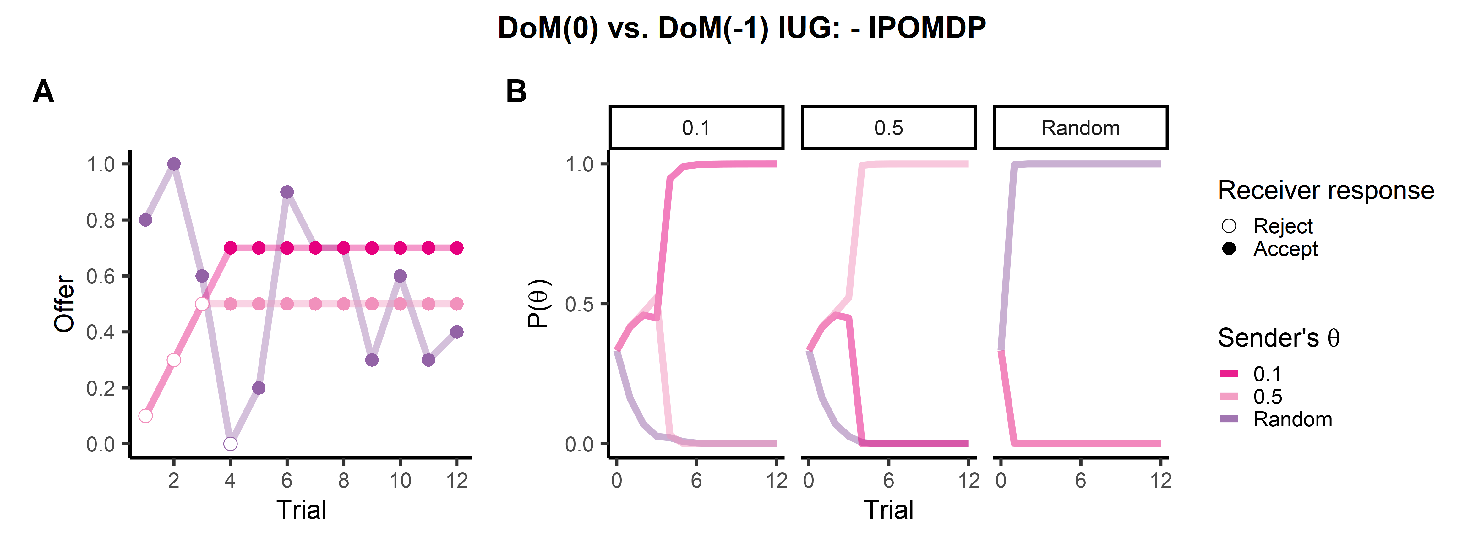
Figure 5: DoM$(0)$ vs DoM$(-1)$ in IUG IPOMDP: (A) Interacting with a DoM$(-1)$, the DoM$(0)$ quickly infers the type of the $\alpha_{-1}$ from its first actions. The DoM$(-1)$ threshold sender first offer tell it apart from the random sender as its initial offer is always $0$. The DoM$(0)$ policy is a function of its updates beliefs (B). When engaging with a threshold DoM$(-1)$ sender, it rejects the offers until the sender is unwilling to “improve” its offers, which also corresponds to the certainty of its beliefs

Using its capacity to fully simulate this behaviour, the DoM$(1)$ sender acts deceptively by masquerading as a random sender. This preys on the lack of agency that the DoM$(0)$ has over the random sender. This ruse is characterized by a signature move, depicted in Fig. 2. The sender begins by making a relatively high offer (Fig. 2(A)). This offer is very unlikely for the threshold DoM$(-1)$ senders, hence the belief update of the DoM$(0)$ receiver strongly favours the random sender hypothesis (Fig. 2(B)). Once the receiver’s beliefs are misplaced, the sender takes advantage of the statistical nature of the random sender policy—every offer has the same likelihood: $\frac{1}{|\mathcal{A}|}$. This allows the sender to drop their subsequent offers substantially, while avoiding “detection”, since the receiver’s beliefs are fooled by this probabilistic trait.

6.1.2 $\aleph$-IPOMDP parameters in IUG

Simulating this interaction as a $\aleph$-IPOMDP allows us to illustrate how the $\aleph$-mechanism detects the masquerading sender and how the $\aleph$-policy deters it from doing so. We set the general parameters $\mathcal{T}=0.1,\gamma=0.99$ and the $\aleph$-mechanism parameters: $\delta(t)=\max\{\nicefrac{{(T-t)}}{{t}},0.5\}$ and set $\omega=1.5$. Notably, $\delta(t)$ is a function of the duration of the interaction. Typically $\delta$ is a fixed, small size. However, due to the sequential nature of the interaction, it seems implausible to set this size in this matter for the following reason: the empirical distribution is a function of the sample size as well, hence the size of the strong typical set varies with sample size. At the limit $\lim_{t\rightarrow T}\delta(t)\rightarrow 0$. To increase the set of $\delta$-strong typicality trajectories we bound this limit by $0.5$—this means that the size of the set (Eq. 7) decreases with time, but remains wide enough. Future work can explore the interaction between these parameters and find an optimal way of tuning them.

6.2 Iterated Bayesian zero-sum game

In this game a payout matrix (Eq. 9) is selected randomly (with equal probability) and remains fixed throughout the interaction. The game is played for $T>0$ trials. In each trial the row player picks one of two actions $a_{\alpha}\in\{T,B\}$, corresponding to either the top row or the bottom one, and the column player picks one of the columns: $a_{\beta}\in\{L,M,R\}$. The agents pick actions simultaneously and observe the action selected by the opponent before the next trial begins. As in the original paper, the payoffs were hidden and revealed only at the end of the game to avoid disclosing the game played.

The row player may or may not know which matrix is selected (this event too is uniformly distributed). We denote the row player type by $\theta_{\alpha}\in\{0,1,2\}$, where $0$ corresponds to zero knowledge of the game, $\theta_{\alpha}\in\{1,2\}$ indicates that $\alpha$ knows which game is played. Formally: $P(\theta_{\alpha}=0)=P(\theta_{\alpha}\in\{1,2\})=\nicefrac{{1}}{{2}}$. By contrast, $\beta$ is oblivious to the selection, but draws inferences about it from the behaviour of $\alpha$, as described next.

In this game we simulate 2 types of row players: either with DoM level $k\in\{-1,1\}$. We also consider 2 types of $\beta$’s DoM level $\{0,2\}$. The DoM$(-1)$ $\alpha$ follows a simple policy. If $\theta_{\alpha_{-1}}\in\{1,2\}$, meaning that the row player knows which payoff matrix is selected, they pick an action via SoftMax policy (Equation 5) of the Q-values (assuming uniform column distribution):

$$Q_{\alpha_{-1}}(a_{\alpha}|\theta_{\alpha_{-1}})=E_{a_{\beta}\sim U}[u_{\alpha}(a_{\alpha},a_{\beta})]$$ (16)

Else it uniformly randomizes between the columns.

Knowing this, $\beta_{0}$ applies IRL to make inferences about the game played from $\alpha$’s actions:

$$b^{t}_{\beta_{0}}(\theta_{\alpha_{-1}})=p(\theta_{\alpha_{-1}}|h^{t})\propto P(a_{\alpha}^{t}|\theta_{\alpha_{-1}})p(\theta_{\alpha_{-1}}|h^{t-1})$$ (17)

We assume a flat prior over the row player’s type. An illustration of this IRL is presented in Fig. 6(A). In this example, the payout matrix is $G_{1}$, and $\theta_{\alpha_{-1}}=1$, that is, the row player is informed about the payout matrix. In this case, the DoM$(-1)$ Q-values are $Q_{\alpha_{-1}}(T|\theta_{\alpha_{-1}}=1)=2$ and $Q_{\alpha_{-1}}(B|\theta_{\alpha_{-1}}=1)=\nicefrac{{2}}{{3}}$, implying that $T$ is the most likely action for it. In turn, the DoM$(0)$ column player is quick to detect this and its optimal policy is to select the column that yields it $0$ reward.

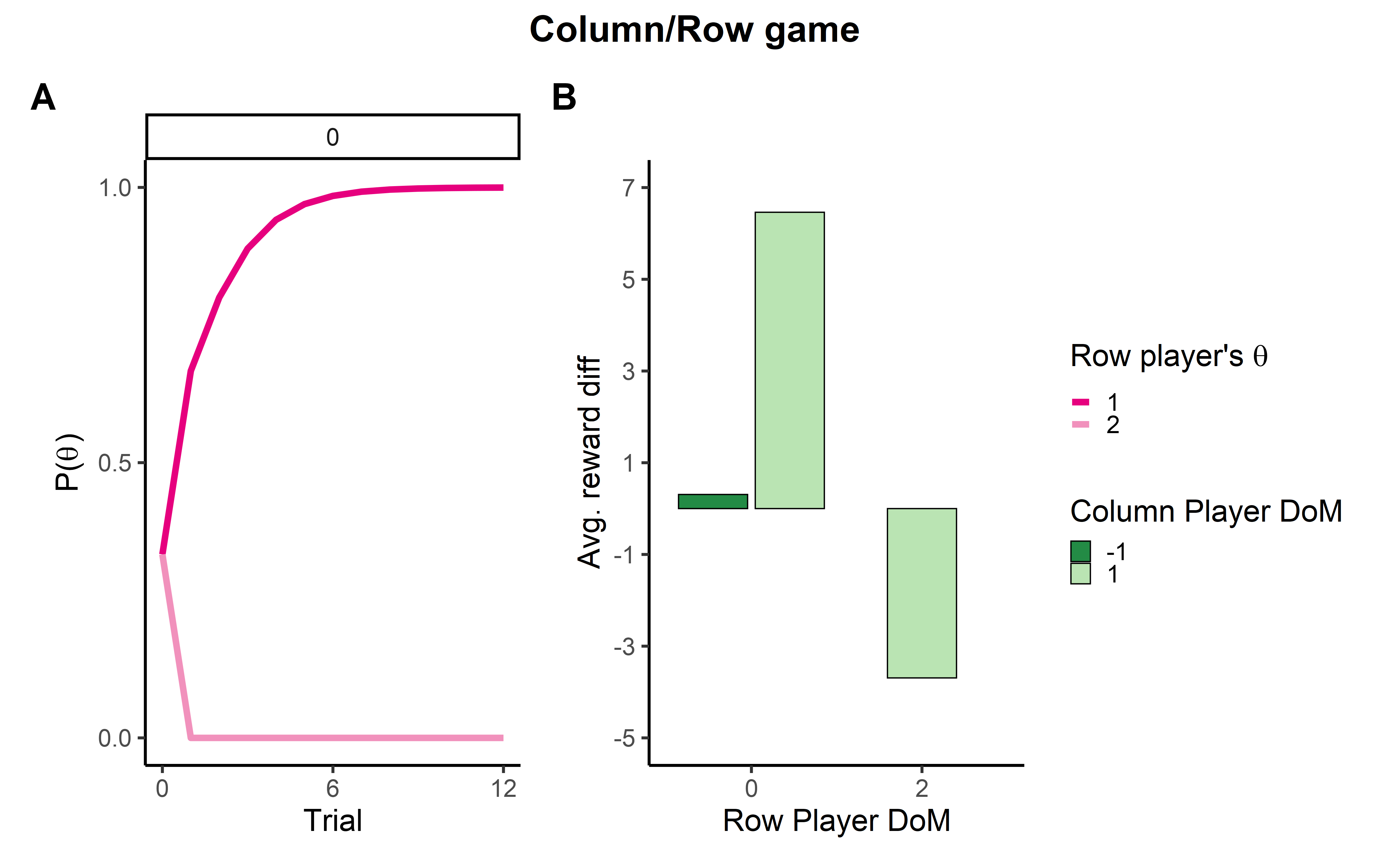
Figure 6: Row/Column zero-sum game: (A) Illustration of DoM$(0)$ Bayesian-IRL. Given the row player’s actions, the DoM$(0)$ column player quickly detects the true type (and payoff matrix). (B) Advantage of high DoM level: in each of the simulated dyads, the higher DoM agent has an edge. Its ability to simulate and predict its opponent’s behaviour allows it to gain excess wealth

The DoM$(1)$ row player make inferences about the DoM$(0)$ player IRL and plans through its belief update and optimal policy to maximize its reward:

$$Q(a^{t}_{\alpha}|h^{t},\theta_{\alpha_{1}})=E_{a_{\beta}\sim\pi^{*}_{\beta_{0}}}[u_{\alpha}(a_{\alpha},a_{\beta})|h^{t}]$$ (18)

where $\pi^{*}_{\beta_{0}}$ is $\beta_{0}$ optimal policy after observing $a^{t}_{\alpha}$. Lastly, the DoM$(2)$ models the row player as a DoM$(1)$. It inverts its actions to make inference about the payoff matrix from and act optimally, similarly to the DoM$(0)$.

6.2.1 Manipulation, counter manipulation and counter-counter manipulation

We begin by simulating the game as an IPOMDP. The DoM$(1)$ row player infers through simulation how to deceive the DoM$(0)$ by manipulating the latter’s beliefs. In this task, it acts in a way that signals that it knows which payoff matrix had been chosen, but in a way that causes the DoM$(0)$ to form false beliefs about the matrix. For example, if the true matrix is $G_{1}$, the DoM$(1)$ row player selects the bottom row ($a_{\alpha}=B$), a typical behaviour for $\theta_{-1}=2$ (as this row has the highest expected reward in $G_{2}$). In turn, the DoM$(0)$ picks the left column, mistakenly believing that they are rewarded with $0$. This ploy yields a reward of $4$ to the DoM$(1)$ player, resulting in a high income gap in its favour, as illustrated in Fig. 6(B). Remarkably, this policy exposes $\alpha_{1}$ to potential risk as the right column yields it a negative reward. However, given its ability to predict the DoM$(0)$ row player’s action this risk is mitigated. Being aware of this ruse, the DoM$(2)$ column player tricks the trickster by learning to select the right column. The DoM$(2)$ take advantage of the DoM$(1)$ inability to model its behaviour as deceptive and resent it, which yields it a reward of $2$ at each trial, depicted in Fig. 6(B).

We solve this issue by simulating the game again using the $\aleph$-IPOMDP framework. Due to the reward masking, the DoM$(1)$ detects that they are matched with an external opponent only through the typical-set component. Identifying that they are outmatched, the $\aleph$-policy is to play the MinMax policy—selecting the row that yields the highest-lowest reward. Interestingly, in this task, this policy is similar to the optimal policy of the “truth-telling” DoM$(-1)$ agent. In this case the DoM$(2)$ respond is to select the column which yields it the highest reward—namely the one that yields it a zero reward, as evident in 4(C).

References

- Alon et al. [2023a] Nitay Alon, Lion Schulz, Peter Dayan, and Joseph M Barnby. Between prudence and paranoia: Theory of mind gone right, and wrong. In First Workshop on Theory of Mind in Communicating Agents, 2023a. URL https://openreview.net/forum?id=gB9zrEjhZD.
- Alon et al. [2023b] Nitay Alon, Lion Schulz, Jeffrey S. Rosenschein, and Peter Dayan. A (dis-) information theory of revealed and unrevealed preferences: Emerging deception and skepticism via theory of mind. Open Mind, 7:608–624, 2023b.
- Barnby et al. [2023] Joseph M Barnby, Peter Dayan, and Vaughan Bell. Formalising social representation to explain psychiatric symptoms. Trends in Cognitive Sciences, 2023.
- Camerer [2011] Colin F Camerer. Behavioral game theory: Experiments in strategic interaction. Princeton university press, 2011.
- Camerer et al. [2004] Colin F. Camerer, Teck-Hua Ho, and Juin-Kuan Chong. A Cognitive Hierarchy Model of Games*. The Quarterly Journal of Economics, 119(3):861–898, August 2004. ISSN 0033-5533. doi: 10.1162/0033553041502225. URL https://doi.org/10.1162/0033553041502225.
- Doshi et al. [2014] Prashant Doshi, Xia Qu, and Adam Goodie. Chapter 8 - Decision-Theoretic Planning in Multiagent Settings with Application to Behavioral Modeling. In Gita Sukthankar, Christopher Geib, Hung Hai Bui, David V. Pynadath, and Robert P. Goldman, editors, Plan, Activity, and Intent Recognition, pages 205–224. Morgan Kaufmann, Boston, January 2014. ISBN 978-0-12-398532-3. doi: 10.1016/B978-0-12-398532-3.00008-7. URL https://www.sciencedirect.com/science/article/pii/B9780123985323000087.
- Ebrahimi et al. [2018] Javid Ebrahimi, Anyi Rao, Daniel Lowd, and Dejing Dou. HotFlip: White-Box Adversarial Examples for Text Classification, May 2018. URL http://arxiv.org/abs/1712.06751. arXiv:1712.06751 [cs].
- Evans et al. [2007] Scott Evans, Earl Eiland, Stephen Markham, Jeremy Impson, and Adam Laczo. Mdlcompress for intrusion detection: Signature inference and masquerade attack. In MILCOM 2007 - IEEE Military Communications Conference, pages 1–7, 2007. doi: 10.1109/MILCOM.2007.4455304.
- Foerster et al. [2018] Jakob N. Foerster, Richard Y. Chen, Maruan Al-Shedivat, Shimon Whiteson, Pieter Abbeel, and Igor Mordatch. Learning with Opponent-Learning Awareness. arXiv:1709.04326 [cs], September 2018. URL http://arxiv.org/abs/1709.04326. arXiv: 1709.04326.
- Friedman [1971] James W Friedman. A non-cooperative equilibrium for supergames. The Review of Economic Studies, 38(1):1–12, 1971.
- Frith and Frith [2021] Chris D Frith and Uta Frith. Mapping mentalising in the brain. In The neural basis of mentalizing, pages 17–45. Springer, 2021.
- Gmytrasiewicz and Doshi [2005] P. J. Gmytrasiewicz and P. Doshi. A Framework for Sequential Planning in Multi-Agent Settings. Journal of Artificial Intelligence Research, 24:49–79, July 2005. ISSN 1076-9757. doi: 10.1613/jair.1579. URL https://jair.org/index.php/jair/article/view/10414.
- Gmytrasiewicz and Adhikari [2019] Piotr J Gmytrasiewicz and Sarit Adhikari. Optimal sequential planning for communicative actions: A bayesian approach. In AAMAS, volume 19, pages 1985–1987, 2019.
- Harsanyi [1968] John C. Harsanyi. Games with incomplete information played by ”bayesian” players, i-iii. part iii. the basic probability distribution of the game. Management Science, 14(7):486–502, 1968. ISSN 00251909, 15265501. URL http://www.jstor.org/stable/2628894.
- Hula et al. [2015] Andreas Hula, P. Read Montague, and Peter Dayan. Monte Carlo Planning Method Estimates Planning Horizons during Interactive Social Exchange. PLOS Computational Biology, 11(6):e1004254, June 2015. ISSN 1553-7358. doi: 10.1371/journal.pcbi.1004254. URL https://journals.plos.org/ploscompbiol/article?id=10.1371/journal.pcbi.1004254. Publisher: Public Library of Science.
- Hula et al. [2018] Andreas Hula, Iris Vilares, Terry Lohrenz, Peter Dayan, and P. Read Montague. A model of risk and mental state shifts during social interaction. PLOS Computational Biology, 14(2):e1005935, February 2018. ISSN 1553-7358. doi: 10.1371/journal.pcbi.1005935. URL https://journals.plos.org/ploscompbiol/article?id=10.1371/journal.pcbi.1005935. Publisher: Public Library of Science.
- Le Guillarme et al. [2016] Nicolas Le Guillarme, Abdel-Illah Mouaddib, Sylvain Gatepaille, and Amandine Bellenger. Adversarial Intention Recognition as Inverse Game-Theoretic Planning for Threat Assessment. In 2016 IEEE 28th International Conference on Tools with Artificial Intelligence (ICTAI), pages 698–705, November 2016. doi: 10.1109/ICTAI.2016.0111. URL https://ieeexplore.ieee.org/document/7814671. ISSN: 2375-0197.
- Liebald et al. [2007] Benjamin Liebald, Dan Roth, Neelay Shah, and Vivek Srikumar. Proactive Detection of Insider Attacks. Technical Report UIUCDCS-R-2007-2879, University of Illinois, 2007.
- Maguire et al. [2019] Phil Maguire, Philippe Moser, Rebecca Maguire, and Mark T Keane. Seeing patterns in randomness: A computational model of surprise. Topics in cognitive science, 11(1):103–118, 2019.
- McNamara and Houston [2002] John M McNamara and Alasdair I Houston. Credible threats and promises. Philosophical Transactions of the Royal Society of London. Series B: Biological Sciences, 357(1427):1607–1616, 2002.
- Milgrom [1984] Paul R Milgrom. Axelrod’s” the evolution of cooperation”, 1984.
- Nachbar and Zame [1996] John H Nachbar and William R Zame. Non-computable strategies and discounted repeated games. Economic theory, 8:103–122, 1996.
- Ng and Russell [2000] Andrew Y. Ng and Stuart Russell. Algorithms for Inverse Reinforcement Learning. In in Proc. 17th International Conf. on Machine Learning, pages 663–670. Morgan Kaufmann, 2000.
- Nowak and Sigmund [1992] Martin A Nowak and Karl Sigmund. Tit for tat in heterogeneous populations. Nature, 355(6357):250–253, 1992.
- Obaidat et al. [2019] Mohammad S Obaidat, Issa Traore, and Isaac Woungang. Biometric-based physical and cybersecurity systems. Springer, 2019.
- Pacuit and Roy [2017] Eric Pacuit and Olivier Roy. Epistemic Foundations of Game Theory. In Edward N. Zalta, editor, The Stanford Encyclopedia of Philosophy. Metaphysics Research Lab, Stanford University, summer 2017 edition, 2017. URL https://plato.stanford.edu/archives/sum2017/entries/epistemic-game/.
- Palomäki et al. [2016] Jussi Palomäki, Jeff Yan, and Michael Laakasuo. Machiavelli as a poker mate — A naturalistic behavioural study on strategic deception. Personality and Individual Differences, 98:266–271, August 2016. ISSN 0191-8869. doi: 10.1016/j.paid.2016.03.089. URL https://www.sciencedirect.com/science/article/pii/S0191886916302434.
- Pannell and Ashman [2010] Grant Pannell and Helen Ashman. User Modelling for Exclusion and Anomaly Detection: A Behavioural Intrusion Detection System. In Paul De Bra, Alfred Kobsa, and David Chin, editors, User Modeling, Adaptation, and Personalization, pages 207–218, Berlin, Heidelberg, 2010. Springer. ISBN 978-3-642-13470-8. doi: 10.1007/978-3-642-13470-8˙20.
- Peng et al. [2016] Jian Peng, Kim-Kwang Raymond Choo, and Helen Ashman. User profiling in intrusion detection: A review. Journal of Network and Computer Applications, 72:14–27, September 2016. ISSN 1084-8045. doi: 10.1016/j.jnca.2016.06.012. URL https://www.sciencedirect.com/science/article/pii/S1084804516301412.
- Premack and Woodruff [1978] David Premack and Guy Woodruff. Does the chimpanzee have a theory of mind? Behavioral and brain sciences, 1(4):515–526, 1978.
- Ramachandran and Amir [2007] Deepak Ramachandran and Eyal Amir. Bayesian inverse reinforcement learning. In Proceedings of the 20th international joint conference on Artifical intelligence, IJCAI’07, pages 2586–2591, San Francisco, CA, USA, January 2007. Morgan Kaufmann Publishers Inc.
- [32] Miquel Ramırez and Hector Geffner. Goal Recognition over POMDPs: Inferring the Intention of a POMDP Agent.
- Rosenberg et al. [2021] Ishai Rosenberg, Asaf Shabtai, Yuval Elovici, and Lior Rokach. Adversarial machine learning attacks and defense methods in the cyber security domain. ACM Computing Surveys (CSUR), 54(5):1–36, 2021.
- Russell [2010] Stuart J Russell. Artificial intelligence: A modern approach. Pearson Education, Inc., 2010.
- Salem et al. [2008] Malek Ben Salem, Shlomo Hershkop, and Salvatore J. Stolfo. A Survey of Insider Attack Detection Research. In Salvatore J. Stolfo, Steven M. Bellovin, Angelos D. Keromytis, Shlomo Hershkop, Sean W. Smith, and Sara Sinclair, editors, Insider Attack and Cyber Security: Beyond the Hacker, Advances in Information Security, pages 69–90. Springer US, Boston, MA, 2008. ISBN 978-0-387-77322-3. doi: 10.1007/978-0-387-77322-3˙5. URL https://doi.org/10.1007/978-0-387-77322-3_5.
- Sarkadi [2023] Stefan Sarkadi. An Arms Race in Theory-of-Mind: Deception Drives the Emergence of Higher-level Theory-of-Mind in Agent Societies. In 4th IEEE International Conference on Autonomic Computing and Self-Organizing Systems ACSOS 2023. IEEE Computer Society, 2023.
- Sarkadi et al. [2019a] Stefan Sarkadi, Alison R. Panisson, Rafael H. Bordini, Peter McBurney, Simon Parsons, and Martin Chapman. Modelling deception using theory of mind in multi-agent systems. AI Communications, 32(4):287–302, January 2019a. ISSN 0921-7126. doi: 10.3233/AIC-190615. URL https://content.iospress.com/articles/ai-communications/aic190615. Publisher: IOS Press.
- Sarkadi et al. [2019b] Ştefan Sarkadi, Alison R. Panisson, Rafael H. Bordini, Peter McBurney, Simon Parsons, and Martin Chapman. Modelling deception using theory of mind in multi-agent systems. AI Communications, 32(4):287–302, January 2019b. ISSN 0921-7126. doi: 10.3233/AIC-190615. URL https://content.iospress.com/articles/ai-communications/aic190615. Publisher: IOS Press.
- Sarkadi et al. [2021] Ştefan Sarkadi, Alex Rutherford, Peter McBurney, Simon Parsons, and Iyad Rahwan. The evolution of deception. Royal Society Open Science, 8(9):201032, September 2021. doi: 10.1098/rsos.201032. URL https://royalsocietypublishing.org/doi/full/10.1098/rsos.201032. Publisher: Royal Society.
- Savas et al. [2022] Yagiz Savas, Christos K. Verginis, and Ufuk Topcu. Deceptive Decision-Making under Uncertainty. Proceedings of the AAAI Conference on Artificial Intelligence, 36(5):5332–5340, June 2022. ISSN 2374-3468. doi: 10.1609/aaai.v36i5.20470. URL https://ojs.aaai.org/index.php/AAAI/article/view/20470. Number: 5.
- Shannon [1993] Claude E Shannon. Programming a computer for playing chess. In first presented at the National IRE Convention, March 9, 1949, and also in Claude Elwood Shannon Collected Papers, pages 637–656. IEEE Press, 1993.
- Yu et al. [2021] Xiaopeng Yu, Jiechuan Jiang, Haobin Jiang, and Zongqing Lu. Model-Based Opponent Modeling. arXiv:2108.01843 [cs], August 2021. URL http://arxiv.org/abs/2108.01843. arXiv: 2108.01843.
- Zamir [1992] Shmuel Zamir. Chapter 5 Repeated games of incomplete information: Zero-sum. In Handbook of Game Theory with Economic Applications, volume 1, pages 109–154. Elsevier, January 1992. doi: 10.1016/S1574-0005(05)80008-6. URL https://www.sciencedirect.com/science/article/pii/S1574000505800086.