Anisotropic Magnetized Asteroseismic Waves

Abstract

We solve for waves in a polytropic, stratified medium with a spatially varying background magnetic field that points along a horizontal $x$-direction, and with gravity that is directed along the vertical $z$-direction. Force balance determines the magnitude of the background magnetic field, $B_{\rm 0}^{2}\sim z^{n+1}$, where $n$ is the polytropic index. Using numerical and asymptotic methods, we deduce an accurate and explicit dispersion relation for fast pressure-driven waves: $\Omega^{2}\sim K\left(2m+n\right)\left[1+(1/\mbox{M}_{\rm A})^{2}(4-2\gamma+\cos^{2}\theta-3\cos^{4}\theta)/4\right]$. Here, $\Omega$ is the frequency, $K$ the wavenumber, $\theta$ the angle the wave-vector makes with the background magnetic field, $\mbox{M}_{\rm A}$ the Alfvénic Mach number, and $m$ an integer representing the eigen state. Applications of our result are in magnetoseismology and nonlinear asteroseismology.

1 Introduction

The strengths of magnetic fields buried below the surface of stars are not known, though they are vital for improved understanding of the magnetic behaviour of stars. This challenge has impeded progress in the development of stellar magnetism and the evolution of magnetized stellar interiors. To estimate the magnetic field strengths, linear asteroseismology has stood as a promising candidate (Aerts et al., 2010), although nonlinear asteroseismology may also be able to provide insights. It is undisputed that the asteroseismology, both linear and nonlinear, benefits from reliable and simple expressions of anisotropic magnetic effect on linear waves. Specifically, the development of nonlinear asteroseismology (Guo, 2020; Van Beeck et al., 2021, 2023) requires linear dispersion relations to evaluate mode resonances; the linear asteroseismology directly employs dispersion relations to solve the inverse problem of detecting subsurface magnetic fields using observed stellar surface oscillations. Such magnetoseismology has witnessed fitful progress. For example, observational studies report travel-time perturbations of acoustic waves to be a critical signature of strong magnetic fields in the stellar interior (Schunker et al., 2005; Ilonidis et al., 2011). Numerical simulations of asteroseismic waves also suggest the possibility of detecting deep-seated fields, before they emerge on the surface (Singh et al., 2014, 2015, 2016, 2020; Das et al., 2020; Das, 2022). To bolster such suggestive findings, a thorough understanding of the impact of magnetic fields on asteroseismic waves is essential (Nye & Thomas, 1976; Adam, 1977; Thomas, 1983; Campos, 1983; Cally, 2007; Campos & Marta, 2015; Tripathi & Mitra, 2022).

Waves in an unmagnetized polytropic atmosphere were exactly solved analytically by Lamb (1911) who derived the relation

$$\frac{\Omega^{2}}{2K}-\frac{(n+1)(n+1-\gamma n)K}{2\gamma^{2}\Omega^{2}}=m+\frac{n}{2},$$ (1)

where $\Omega$ is the frequency, $K$ the wavenumber, $n$ the polytropic index, $\gamma$ the adiabatic index, and $m$ the eigen-state index, with $m=0,1,2,...\,$. This advancement led to a series of newer and significant understanding of hydrodynamic waves. Under fast-wave approximation, $\Omega^{2}/K\gg 1$, the leading-order dispersion relation becomes

$$\Omega^{2}\sim K\left(2m+n\right)\/.$$ (2)

A similar closed-form expression for waves in a magnetized polytrope, as of yet, is unknown. Despite several progresses (e.g., Gough & Thompson, 1990; Bogdan & Cally, 1997; Cally & Bogdan, 1997), the problem, to this day, remains unsolved. Gough & Thompson (1990) treat a global problem (in spherical coordinates); there, the computation of eigenfrequenices requires numerical evaluation of complicated integral expressions [e.g., Eqs. (4.11)–(4.13) in Gough & Thompson (1990)]. A closed-form analytical formula is not available. The limitations of purely numerical approach and lack of a closed-form expression were succinctly expressed by Bogdan & Cally (1997):

“Ideally, we would wish to proceed by writing down an equation analogous to Lamb’s formula for the magnetized polytrope. Unfortunately, this approach is not feasible and for the most part one must instead be content with a numerically derived visual comparison of how the allowed oscillation frequencies depend upon the choice of the horizontal wavenumber $k$.”

Analytic dispersion relations are also essential for developing wave turbulence theory in the presence of both gravity and magnetic fields. In wave turbulence theory, calculations of mode resonances require simple, explicit dispersion relations that accurately capture the magnetic effect on observed linear waves. We note that the Lamb’s dispersion relation (2), $\Omega\sim\sqrt{K}$, is similar to that of surface gravity waves in oceans (Hasselmann, 1962). However, there is a critical difference: the surface gravity waves do not couple via three-wave resonance, thus requiring a weaker four-wave coupling (Nazarenko & Lukaschuk, 2016). The Lamb waves, on the other hand, can couple via three-wave resonance, because there are infinitely many such waves (eigen states) at a given wave number, unlike only one pair of surface gravity waves at a given wave number. Thus, the infinitely many Lamb waves at a given wavenumber have distinct wave frequencies, which allow the sum of three frequencies at three wavenumbers to become null. While a wave turbulence theory for surface gravity waves has been well established, it is yet to be developed for the asteroseismic waves, whose dispersion relation in fully analytic form is a basic requirement for such a theory. The value that an analytic dispersion relation offers in resonant-coupling theory cannot be overstated when magnetic fields make the wave dispersion relation anisotropic and complicated. Motivated by these reasons, we seek here an accurate and simple formulae for the effect of magnetic fields on the Lamb waves.

Introducing magnetic fields, aligned orthogonal to a vertical gravity (Fig. 1), we find, as did Bogdan & Cally (1997), that the linearized magnetohydrodynamic (MHD) equations are too cumbersome to obtain a closed-form expression for the dispersion relation, even with the fast-wave approximation, $\Omega^{2}/K\gg 1$. Here, we overcome this difficulty by using both numerical simulations and extensive use of Mathematica, followed by a variant of Jeffereys–Wentzel–Kramers–Brillouin (JWKB) approximation to deduce

$$\Omega^{2}\sim K\left(2m+n\right)\left[1+\frac{{\mathbb{\color[rgb]{0,0,0}\epsilon}}^{2}(4-2\gamma+\cos^{2}\theta-3\cos^{4}\theta)}{4}\right],$$ (3)

in the limit $\Omega^{2}/K\gg 1$, with $m=0,1,2,...\,$. The parameter ${\mathbb{\color[rgb]{0,0,0}\epsilon}}$ is the inverse of the Alfvénic Mach number and $\theta$ is the angle the wave vector makes with the background magnetic field. Equation (3) is the principal result of this paper.

This paper is organized in the following way. In § 2, we describe our model and present the linearized compressible MHD equations. Such equations are then numerically solved in § 3. To obtain analytical understanding of the numerical results, the linearized equations are reduced to a wave equation in § 4. The normal-form wave equation is then perturbatively solved using a variant of the JWKB theory we devise; analytical understanding is gained in § 5. With astrophysical implications and utility of our results, we conclude in § 6.

2 System setup and linearized perturbation equations

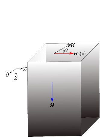
Figure 1: An inhomogeneous magnetic field $\bm{B}_{0}(z)$, oriented orthogonal to a constant vertical gravity $\bm{g}$, is considered where the wave is allowed to propagate in an arbitrary direction, shown with $\bm{K}$, making an angle $\theta$ with $\bm{B}_{0}$. The gradient in the colormap of the box schematically represents increasing functions with depth $z$ of the magnetic field, fluid density, pressure, and sound speed.

To study waves in a magnetized, stratified medium, we consider the ideal compressible MHD equations (Chandrasekhar, 1961)

$$\partial_{t}\rho+{\bm{\nabla}}\cdot\left(\rho{\bm{U}}\right) =0\/,$$ (4a)

$$\rho\left[\partial_{t}{\bm{U}}+({\bm{U}}\cdot\bm{\nabla}){\bm{U}}\right] =-\bm{\nabla}P+\rho\bm{g}+\bm{J}\times\bm{B}\/,$$ (4b)

$$\partial_{t}\bm{B} ={\bm{\nabla}}\times\left({\bm{U}}\times\bm{B}\right),$$ (4c)

$$\frac{Dp}{Dt} =c^{2}\frac{D\rho}{Dt},$$ (4d)

where $\rho$, ${\bm{U}}$, $P$, and $\bm{B}$ represent the density, the velocity, the pressure, and the magnetic field, respectively. The current density is ${\bm{J}}={\bm{\nabla}}\times\bm{B}/\mu_{{\rm 0}}$, where $\mu_{{\rm 0}}$ represents the magnetic permeability of the vacuum. The magnetic field is additionally constrained to be divergence-less

$${\bm{\nabla}}\cdot\bm{B}=0.$$ (5)

We consider a local Cartesian domain where the equilibrium density $\rho_{\rm 0}$ and pressure $P_{\rm 0}$ satisfy the polytropic relation

$$P_{\rm 0}\sim\rho_{\rm 0}^{1+1/n},$$ (6)

where $n$ is the polytropic index of the gaseous atmosphere. In an unmagnetized atmosphere, the force balance gives $\partial_{z}P_{\rm 0}(z)=\rho_{\rm 0}(z)g$, where $\bm{g}=g\hat{\bm{e}}_{z}$, with $g$ as the constant acceleration due to gravity along the vertical $z$-axis, as depicted in Fig. 1. The force balance requires

$$\rho_{\rm 0}(z)\sim z^{n};\quad P_{\rm 0}(z)\sim z^{n+1}.$$ (7)

2.1 Background magnetic field and sound speed

We introduce an inhomogeneous background magnetic field, $\bm{B}=B_{\rm 0}(z)\hat{\bm{e}}_{x}$. The force-balance relation with the Lorentz force, $({\bm{\nabla}}\times\bm{B}/\mu_{{\rm 0}})\times\bm{B}$, then becomes

$$\partial_{z}P_{\rm 0}=\rho_{\rm 0}g-\frac{1}{2\mu_{{\rm 0}}}\partial_{z}B_{\rm 0}^{2}.$$ (8)

The solution

$$B_{0}^{2}(z)\sim z^{n+1}\/$$ (9)

also satisfies Eq. (7). The plasma $\beta$ is then a constant throughout the domain

$$\beta\equiv\frac{P_{\mathrm{gas}}}{P_{\mathrm{magnetic}}}=\frac{2\mu_{{\rm 0}}P_{\rm 0}}{B_{\rm 0}^{2}}.$$ (10)

The sound speed ($c$) may now be deduced from Eq. (8), using $P_{\rm 0}=c^{2}\rho_{\rm 0}/\gamma$, where $\gamma$ is the adiabatic index of the gas

$$\partial_{z}c^{2}=-\frac{nc^{2}}{z}+\frac{\gamma g}{1+\beta^{-1}}.$$ (11)

The solution to Eq. (11) is $c^{2}\mathrm{=}c_{\rm 0}^{2}z$, where $c_{\rm 0}^{2}$ is a constant given by

$$c_{\rm 0}^{2}=\frac{\gamma g}{(n+1)(1+\beta^{-1})}\/.$$ (12)

It is useful to express $\beta^{-1}$ in terms of the Alfvénic Mach number $\mbox{M}_{\rm A}$, which is the ratio of the Alfvén speed to the sound speed,

$$\beta^{-1}=\frac{B_{\rm 0}^{2}}{\mu_{0}\rho_{0}}\cdot\frac{\rho_{0}}{\gamma P_{\rm 0}}\cdot\frac{\gamma}{2}=\frac{\gamma}{2\mbox{M}_{\rm A}^{2}}\/,$$ (13)

using which the sound speed becomes

$$c^{2}=\frac{\gamma gz}{(n+1)(1+\gamma\mbox{M}_{\rm A}^{-2}/2)}.$$ (14)

2.2 Linearized perturbation equations

We now linearize the MHD equations around the background profiles $[\rho_{\rm 0},\bm{0},B_{\rm 0},P_{\rm 0}]$, introduced in Eqs. (7) and (9). Such a linearization yields evolution equations for infinitismal perturbations $[\widetilde{\rho},\widetilde{{\bm{u}}},\widetilde{{\bm{b}}},\widetilde{p}]$ as

$$\partial_{t}\widetilde{\rho} =-(\widetilde{\bm{u}}\cdot\bm{\nabla})\rho_{\rm 0}-\rho_{\rm 0}(\bm{\nabla}\cdot\widetilde{\bm{u}})\/,$$ (15a)

$$\partial_{t}\widetilde{u}_{x} =-\frac{\partial_{x}\widetilde{p}}{\rho_{0}}+\frac{\widetilde{b}_{z}\partial_{z}B_{\rm 0}}{\mu_{{\rm 0}}\rho_{\rm 0}}\/,$$ (15b)

$$\partial_{t}\widetilde{u}_{y} =-\frac{\partial_{y}\widetilde{p}}{\rho_{0}}+\frac{B_{\rm 0}(\partial_{x}\widetilde{b}_{y}-\partial_{y}\widetilde{b}_{x})}{\mu_{{\rm 0}}\rho_{\rm 0}}\/,$$ (15c)

$$\partial_{t}\widetilde{u}_{z} =-\frac{\partial_{z}\widetilde{p}}{\rho_{\rm 0}}+\frac{\widetilde{\rho}g}{\rho_{\rm 0}}+\frac{B_{\rm 0}(\partial_{x}\widetilde{b}_{z}-\partial_{z}\widetilde{b}_{x})-\widetilde{b}_{x}\partial_{z}B_{\rm 0}}{\mu_{{\rm 0}}\rho_{\rm 0}}\/,$$ (15d)

$$\partial_{t}\widetilde{b}_{x} =-B_{\rm 0}(\partial_{y}\widetilde{u}_{y}+\partial_{z}\widetilde{u}_{z})-\widetilde{u}_{z}\partial_{z}B_{\rm 0}\/,$$ (15e)

$$\partial_{t}\widetilde{b}_{y} =-B_{\rm 0}\partial_{x}\widetilde{u}_{y}\/,$$ (15f)

$$\partial_{t}\widetilde{b}_{z} =-B_{\rm 0}\partial_{x}\widetilde{u}_{z}\/,$$ (15g)

$$\partial_{t}\widetilde{p} =-(\widetilde{\bm{u}}\cdot\bm{\nabla})P_{\rm 0}-c^{2}\rho_{0}(\bm{\nabla}\cdot\widetilde{\bm{u}})\/.$$ (15h)

We shall use

$$\widetilde{\chi}=\bm{\nabla}\cdot\widetilde{{\bm{u}}}$$ (16)

in the rest of the article, where helpful.

Equations (15a)–(15h) can be simplified to derive a set of fewer (closed) equations

$$\partial_{t}^{2}\widetilde{u}_{x} =c^{2}\partial_{x}\widetilde{\chi}+g\partial_{x}\widetilde{u}_{z}\/,$$ (17a)

$$\partial_{t}^{2}\widetilde{u}_{y} =c^{2}\partial_{y}\widetilde{\chi}+g\partial_{y}\widetilde{u}_{z}+\frac{c^{2}}{\mbox{M}_{\rm A}^{2}}\left(\partial_{xx}\widetilde{u}_{y}+\partial_{y}\widetilde{\chi}-\partial_{xy}\widetilde{u}_{x}\right)\/,$$ (17b)

$$\partial_{t}^{2}\widetilde{u}_{z} =c^{2}\partial_{z}\widetilde{\chi}-g\partial_{x}\widetilde{u}_{x}\left[1+\frac{\gamma}{\mbox{M}_{\rm A}^{2}(1+\gamma\mbox{M}_{\rm A}^{-2}/2)}\right]-g\partial_{y}\widetilde{u}_{y}$$

$$\hskip 5.69046pt+\frac{\gamma(1+\mbox{M}_{\rm A}^{-2})g\widetilde{\chi}}{(1+\gamma\mbox{M}_{\rm A}^{-2}/2)}+\frac{c^{2}}{\mbox{M}_{\rm A}^{2}}\left(\partial_{xx}\widetilde{u}_{z}+\partial_{z}\widetilde{\chi}-\partial_{xz}\widetilde{u}_{x}\right)\/.$$ (17c)

We note that the appearance of $\mbox{M}_{\rm A}^{2}$ in Eq. (17) in certain terms may seem non-trivial at first sight; however, upon inspection, we understand them as terms emerging from the effect of the Lorentz force on the background states, via terms like $\partial_{z}c^{2}(z)$ and $(\partial_{z}P_{\rm 0})/\rho_{n}$, while processing Eqs. (15a)–(15h). Admittedly, Eqs. (17a)–(17) are somewhat challenging to proceed with clarity. Thus, we now non-dimensionalize the equations to make them reasonably transparent.

2.3 Non-dimensionalized linear equations

We define $L$ as the characteristic length scale over which the sound speed varies (and, for that matter, pressure, density, and temperature also vary) appreciably. Then we find that the characteristic sound speed in an unmagnetized polytrope is, using Eq. (14), $c_{L}=\sqrt{\gamma gL/(n+1)}$. Using $L$ and $L/c_{L}$ as the dimensional length and time units, we non-dimensionalize all variables henceforth, starting with the sound speed

$$C^{2}=\frac{c^{2}}{c_{L}^{2}}=\frac{Z}{1+\gamma\mbox{M}_{\rm A}^{-2}/2},$$ (18)

where the lowercase dimensional variables ($c$ and $z$) are cast as uppercase non-dimensional variables ($C$ and $Z$). Thus we replace all the dimensional variables in Eqs. (17a)–(17) using

$$(x,y,z) =(LX,LY,LZ),$$ (19a)

$$c^{2} =c_{L}^{2}\frac{Z}{1+\gamma\mbox{M}_{\rm A}^{-2}/2},$$ (19b)

$$\partial_{t} \equiv\frac{c_{L}}{L}\partial_{T},$$ (19c)

where the uppercase characters $X,Y,$ and $T$ represent non-dimensional variables.

We analyze perturbations by Fourier-transforming in the $(x,y)$-plane, viz.,

$$\widetilde{u}_{x}(Z)=\int dK_{X}dK_{Y}d\Omega\,\hat{u}_{x}\exp\left[i(K_{X}X+K_{Y}Y+\Omega T)\right],$$ (20)

where the uppercase characters represent non-dimensional quantities, e.g., $\bm{K}\equiv(K_{X},K_{Y})$ is the non-dimensional wavevector in the $(x,y)$-plane, and $\Omega$ is the nondimensional frequency. Fourier analyzing Eqs. (17a)–(17) and representing $\mbox{M}_{\rm A}^{-1}$ by ${\mathbb{\color[rgb]{0,0,0}\epsilon}}$ henceforth, we write

$$\left[\frac{-\Omega^{2}(1+\gamma{\mathbb{\color[rgb]{0,0,0}\epsilon}}^{2}/2)}{iK_{X}Z}\right]\hat{u}_{x}+\left[\frac{-(n+1)(1+\gamma{\mathbb{\color[rgb]{0,0,0}\epsilon}}^{2}/2)}{\gamma Z}\right]\hat{u}_{z}=\hat{\chi}\/,$$ (21a)

$$\left[-i{\mathbb{\color[rgb]{0,0,0}\epsilon}}^{2}K_{X}\right]\hat{u}_{x}+\left[\frac{-\Omega^{2}(1+\gamma{\mathbb{\color[rgb]{0,0,0}\epsilon}}^{2}/2)}{iK_{Y}Z}+\frac{{\mathbb{\color[rgb]{0,0,0}\epsilon}}^{2}K_{X}^{2}}{iK_{Y}}\right]\hat{u}_{y}$$

$$\hskip 56.9055pt+\left[\frac{-(n+1)(1+\gamma{\mathbb{\color[rgb]{0,0,0}\epsilon}}^{2}/2)}{\gamma Z}\right]\hat{u}_{z}=\hat{\chi}(1+{\mathbb{\color[rgb]{0,0,0}\epsilon}}^{2})\/,$$ (21b)

$$\left[iK_{X}\left\{\frac{1+\gamma{\mathbb{\color[rgb]{0,0,0}\epsilon}}^{2}/2}{\gamma}+{\mathbb{\color[rgb]{0,0,0}\epsilon}}^{2}\left(1+\frac{Z\partial_{Z}}{n+1}\right)\right\}\right]\hat{u}_{x}$$

$$+\left[\frac{iK_{Y}(1+\gamma{\mathbb{\color[rgb]{0,0,0}\epsilon}}^{2}/2)}{\gamma}\right]\hat{u}_{y}+\left[\frac{-\Omega^{2}(1+\gamma{\mathbb{\color[rgb]{0,0,0}\epsilon}}^{2}/2)+{\mathbb{\color[rgb]{0,0,0}\epsilon}}^{2}ZK_{X}^{2}}{n+1}\right]\hat{u}_{z}$$

$$\hskip 99.58464pt=\left(\hat{\chi}+\frac{Z\partial_{Z}\hat{\chi}}{n+1}\right)(1+{\mathbb{\color[rgb]{0,0,0}\epsilon}}^{2})\/.$$ (21c)

3 Exact numerical solution

We obtain fully converged numerical solution to Eqs. (21a)–(21) by employing the spectral code “Dedalus” (Burns et al., 2020). Referring to the Dedalus methods paper (Burns et al., 2020) for more details, we briefly outline the numerical procedures employed in Dedalus for eigenvalue problems. At each horizontal wavenumber $(K_{X},K_{Y})$, the state variables—the three components of velocity—are expanded in the Chebyshev polynomials along the inhomogeneous $z$-axis. Because of the background inhomogeneity, different Chebyshev coefficients couple, creating a dense linear operator. Sparsification is provided by a change of basis from the Chebyshev polynomials of the first kind to those of the second kind. To impose boundary conditions and keep the matrix sparse, Dirichlet preconditioning is applied. Efficient solution of the resulting matrices is then found by passing the matrices $\mathcal{L}$ and $\mathcal{M}$ in the eigenvalue ($\sigma$) problem, $\mathcal{L}\mathcal{X}=\sigma\mathcal{M}\mathcal{X}$, to the “scipy” linear algebra packages. For a given spectral resolution along the $z$-axis, we solve for all the eigenvalues of the matrices. Such a non-targeted, general solution produces eigenmodes of all the linear MHD waves, including the pressure-driven and gravity-driven modes. We specialize in the high-frequency modes to assess the effect of magnetic fields on such pressure-driven modes. We identify the pressure-driven modes by comparing their eigenfrequencies with those predicted by Lamb’s solution.

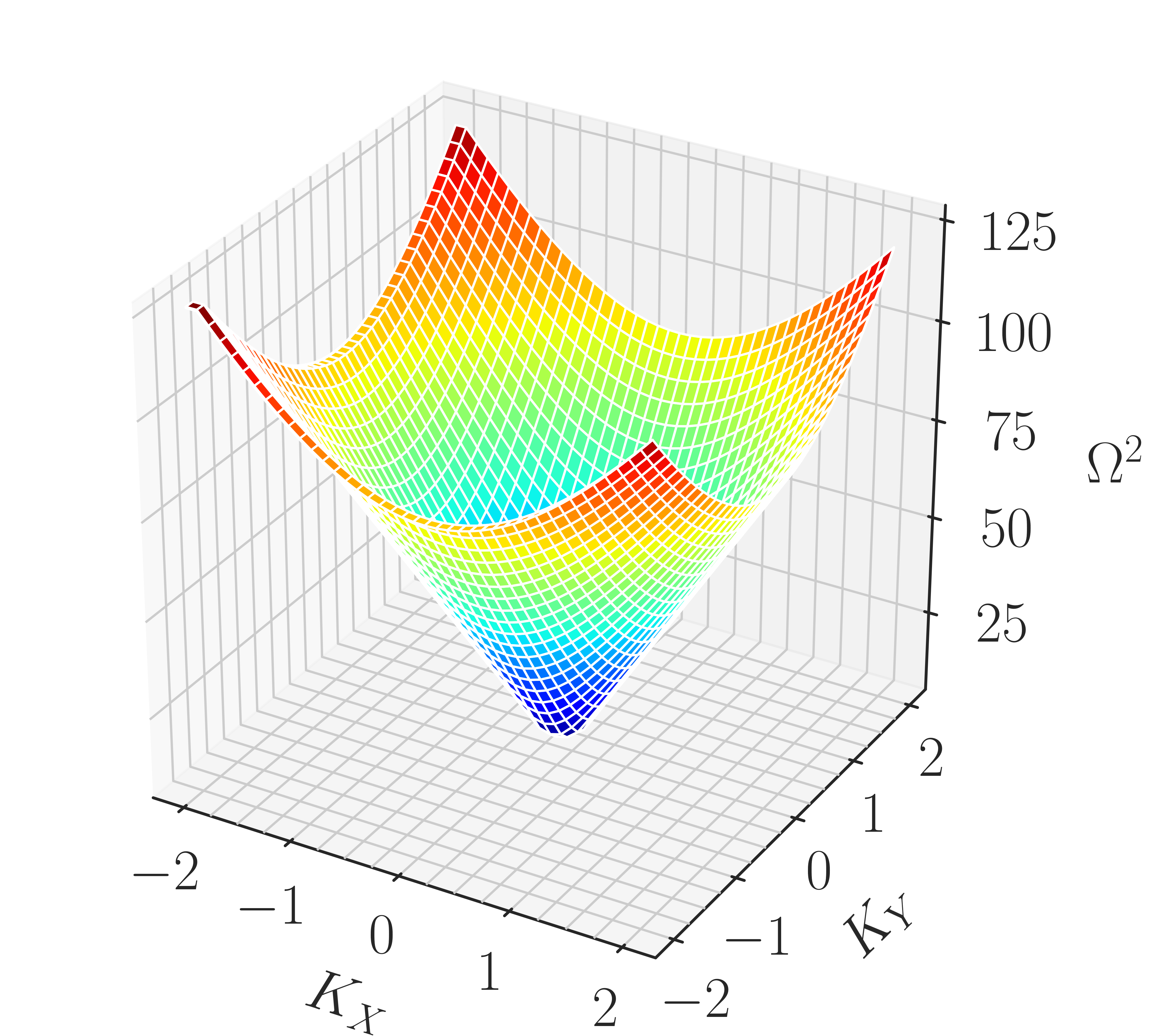
Figure 2: $\Omega^{2}(K_{X},K_{Y})$ for hydrodynamic and magnetized polytropes. The two plotted surfaces are visually indifferentiable because the difference ($\Delta\Omega^{2}$) between them is much smaller than $\Omega^{2}$; see Fig. 3. The parameters used are $\epsilon=0.1$, $m=20$, $n=2.5$, and $\gamma=5/3$. For variations in these parameters, the surface plot of $\Omega^{2}(K_{X},K_{Y})$ remains the same qualitatively.

For the boundary condition, at the lower boundary $z=L_{z}$, we require $\widetilde{u}_{z}=0$. At the upper boundary, $z=0$, where the atmosphere ceases, we enforce, following Lamb (1911),

$$\frac{Dp}{Dt} =0,$$ (22)

which implies

$$c^{2}\frac{D\rho}{Dt}=-c^{2}\rho_{\rm 0}\widetilde{\chi}=0=z^{n+1}\widetilde{\chi}.$$ (23)

We first validate that the solver successfully reproduces Lamb’s exact analytical dispersion relation in the absence of the magnetic field. We then compute the eigenvalues of the magnetized polytrope, which we present in Fig. 2. Although the two surface plots of $\Omega^{2}(K_{X},K_{Y})$ are displayed in Fig. 2—one for the hydrodynamic and other for the magnetized polytrope, the plots are visually indistinguishable. The difference between the two surface plots is shown in Fig. 3. For $K_{Y}=0$, $\Delta\Omega^{2}$ is negative, and for $K_{X}=0$, $\Delta\Omega^{2}$ is positive and relatively large. We also note a minor decrease in positive value of $\Delta\Omega^{2}$ in going from $K_{X}\approx 0$ to $K_{X}=0$.

It turns out that $\Delta\Omega^{2}$ is related to the hydrodynamic squared-frequency $\Omega_{\mathrm{hydro}}^{2}$; and $\Delta\Omega^{2}/\Omega_{\mathrm{hydro}}^{2}$ is almost entirely independent of the wavevector magnitude (Fig. 4). Only angular dependence is observed.

The extremely low wavenumbers in Fig. 4 correspond to very large scale waves that cannot be captured in a finite box in numerical calculation. To capture lower wavenumbers, we significantly extended domain size along the vertical $z$-axis, which allowed us to obtain fully converged numerical results for other wavenumbers.

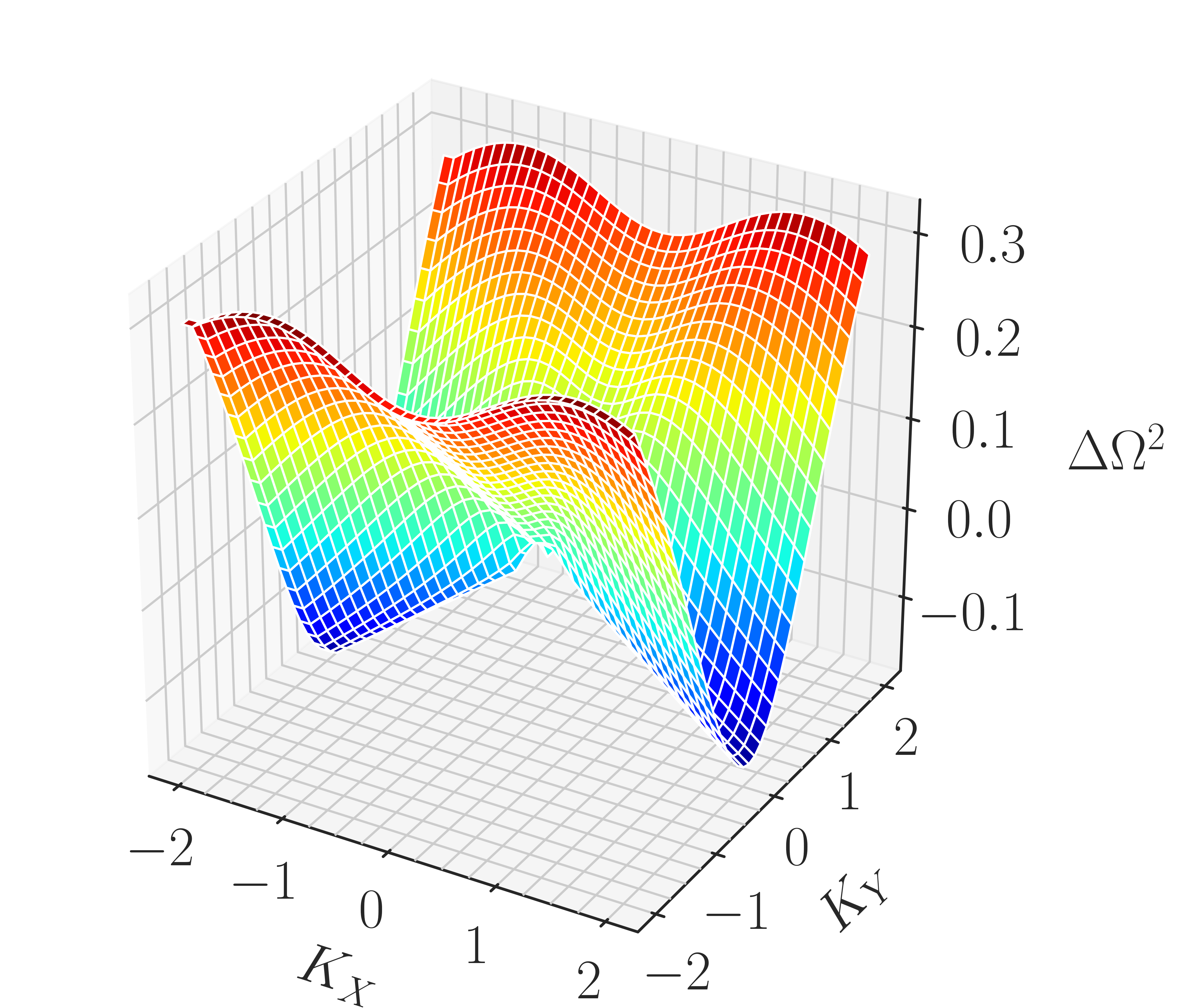
Figure 3: $\Delta\Omega^{2}=\Omega^{2}-\Omega_{\mathrm{hydro}}^{2}$ is plotted for a magnetized polytrope, with $\epsilon=0.1$, $m=20$, $n=2.5$, and $\gamma=5/3$. This surface plot shows the difference between the two surface plots in Fig. 2.

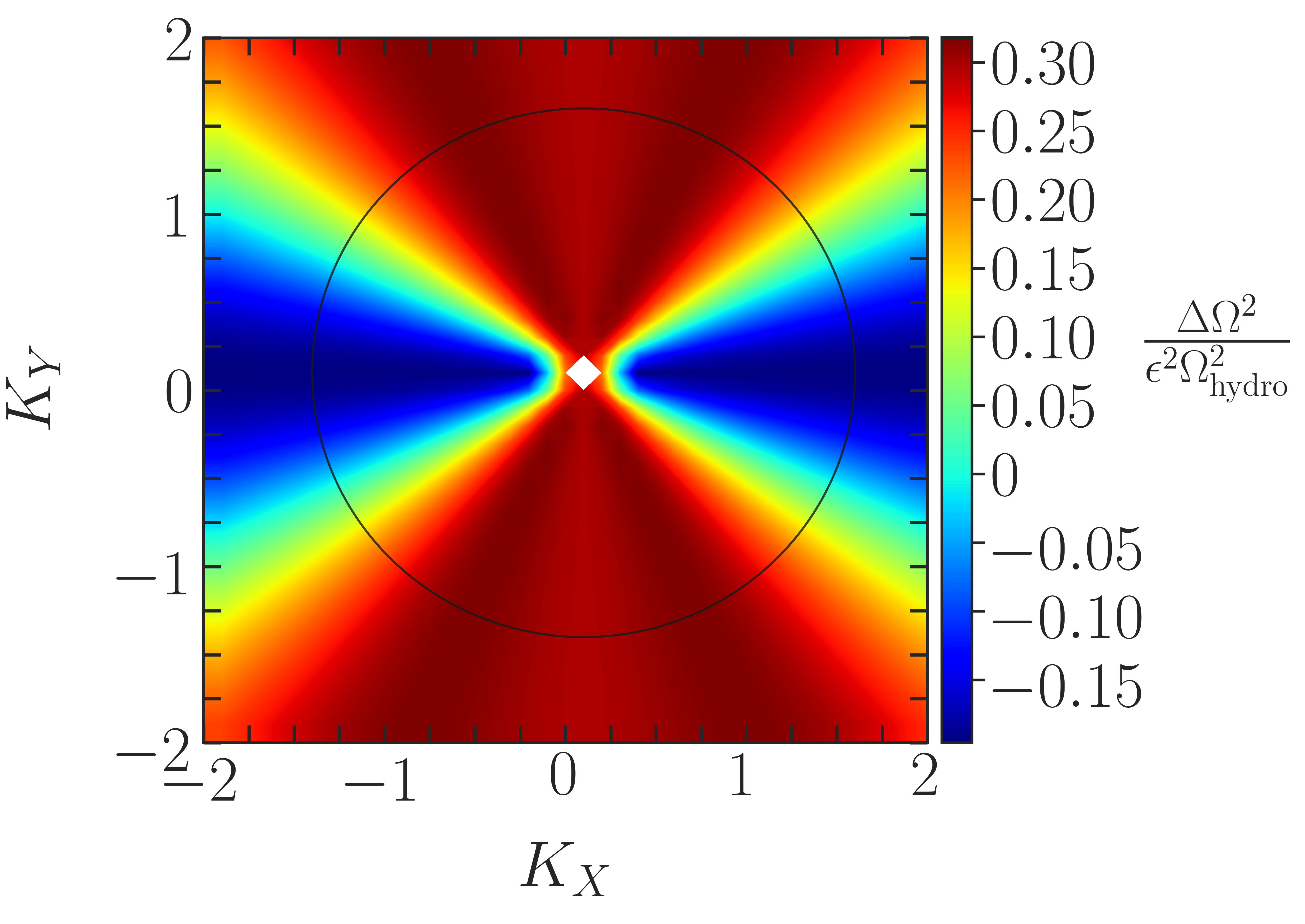
Figure 4: Relative difference of squared-frequency depends on the wavevector propagation angle (spanned by the black circle), but the relative difference is insensitive to the wavevector magnitude. The parameters chosen are $\epsilon=0.1$, $m=20$, $n=2.5$, and $\gamma=5/3$.

4 Reduction to wave equation

To analytically determine the dispersion relation, we solve the set of equations (21a)–(21) perturbatively in the limit of a weak magnetic field, i.e., ${\mathbb{\color[rgb]{0,0,0}\epsilon}}\ll 1$. By setting ${\mathbb{\color[rgb]{0,0,0}\epsilon}}=0$, we recover the Lamb’s equations for the unmagnetized polytrope  (Lamb, 1911). The Lamb’s equations reduce to a second-order differential equation for $\hat{\chi}$. With the same goal, we proceed in the following manner. We rewrite Eqs. (21a)–(21) as

$$\begin{bmatrix}\begin{array}[]{c c c}M_{11}&M_{12}&M_{13}\\ M_{21}&M_{22}&M_{23}\\ M_{31}&M_{32}&M_{33}\\ \end{array}\end{bmatrix}\begin{bmatrix}\begin{array}[]{c}\hat{u}_{x}\\ \hat{u}_{y}\\ \hat{u}_{z}\\ \end{array}\end{bmatrix}=\begin{bmatrix}\begin{array}[]{c}h_{x}(\hat{\chi})\\ h_{y}(\hat{\chi})\\ h_{z}(\hat{\chi},\partial_{Z}\hat{\chi})\\ \end{array}\end{bmatrix},\\$$ (24)

where the matrix elements $M_{ij}$ are independent of $Z$-derivatives, and are functions of $K_{X},K_{Y},\Omega,n,\gamma,{\mathbb{\color[rgb]{0,0,0}\epsilon}},$ and $Z$ only (for their complete expressions, see Appendix A). In arriving at Eq. (24), we have replaced $\partial_{Z}\hat{u}_{x}$ in the first term on the left-hand side of Eq. (21) with its exact expression obtained by differentiating Eq. (21a) with respect to $Z$. We then substitute $\partial_{Z}$ operation in $\partial_{Z}\hat{u}_{z}$ by writing it as $\hat{\chi}-iK_{X}\hat{u}_{x}-iK_{Y}\hat{u}_{y}$. Such a process removes $\partial_{Z}$ operation from the matrix $M$. The functions $h_{\nu}$ are linear in $\hat{\chi}$ and $\partial_{Z}\hat{\chi}$.

Straightforward inversion of the matrix $M$ expresses all components of the velocity in terms of $\hat{\chi}$ and $\partial_{Z}\hat{\chi}$:

$$\hat{u}_{\nu}=f_{\nu}(Z)\hat{\chi}+g_{\nu}(Z)\partial_{Z}\hat{\chi},$$ (25)

where $\nu$ can be either $x,y,$ or $z$. We recognize that $f_{\nu}$ and $g_{\nu}$ are functions of $Z$, but do not involve $\partial_{Z}$. The three velocity components of Eq. (25) can now be subsumed into a single second-order differential equation for $\hat{\chi}$:

$$\partial_{Z}^{2}\hat{\chi}+P(Z,{\mathbb{\color[rgb]{0,0,0}\epsilon}})\partial_{Z}\hat{\chi}+R(Z,{\mathbb{\color[rgb]{0,0,0}\epsilon}})\hat{\chi}=0,$$ (26)

which can be recast into the normal form of the second-order differential equation by changing variable as

$$\hat{\chi}(Z)=\hat{\psi}(Z)\exp{\left[-\frac{1}{2}\int_{Z}dZ\,P(Z)\right]},$$ (27)

which reduces Eq. (26) to the wave equation

$$\partial_{Z}^{2}\hat{\psi}+\Gamma^{2}(Z,{\mathbb{\color[rgb]{0,0,0}\epsilon}})\hat{\psi}=0.$$ (28)

The procedure outlined above appears straightforward. However, the analytical manipulations in arriving at Eq. (28)—a magnetized version of Lamb’s equation—require laborious and careful calculations, as $\Gamma^{2}(Z,{\mathbb{\color[rgb]{0,0,0}\epsilon}})$ alone conceals an expression of exhaustive length—tens of pages of this article. In the absence of the magnetic field, the expression for $\Gamma^{2}(Z,{\mathbb{\color[rgb]{0,0,0}\epsilon}}=0)=\Gamma_{\rm 0}^{2}(Z)$ is beautifully short, $\Gamma_{\rm 0}(Z)=K^{2}(Z-\alpha)(\beta-Z)/Z^{2}$, where $\alpha$ and $\beta$ are the two turning points—two zeros of $\Gamma_{\rm 0}(Z)$.

5 Perturbative solution for anisotropic magnetic effect

The presence of a weak magnetic field may be considered as a perturbation to Lamb’s two-turning point eigenvalue problem. Hence, the magnetic field changes both the locations of the turning points and the form of the potential $\Gamma(Z,{\mathbb{\color[rgb]{0,0,0}\epsilon}})$. In general, we write the JWKB quantization condition (see e.g., Bender & Orszag, 1978; Tripathi, 2022) as

$$\frac{1}{\pi}\int_{Z_{1}({\mathbb{\color[rgb]{0,0,0}\epsilon}})}^{Z_{2}({\mathbb{\color[rgb]{0,0,0}\epsilon}})}\Gamma(Z,{\mathbb{\color[rgb]{0,0,0}\epsilon}})\,dZ\sim\left(m+\frac{1}{2}\right);\,\,\,m=0,1,2,...,$$ (29)

where $m$ refers to the eigen-state index, $\Gamma(Z,{\mathbb{\color[rgb]{0,0,0}\epsilon}})$ is the magnetically-modified wavenumber, and $Z_{1}({\mathbb{\color[rgb]{0,0,0}\epsilon}})$ and $Z_{2}({\mathbb{\color[rgb]{0,0,0}\epsilon}})$ are the magnetically-shifted turning points.

5.1 Perturbative calculations

First, we expand the wavenumber $\Gamma(Z,{\mathbb{\color[rgb]{0,0,0}\epsilon}})$ as

$$\Gamma(Z,{\mathbb{\color[rgb]{0,0,0}\epsilon}})=\Gamma_{\rm 0}(Z)+{\mathbb{\color[rgb]{0,0,0}\epsilon}}\Gamma_{1}(Z)+{\mathbb{\color[rgb]{0,0,0}\epsilon}}^{2}\Gamma_{2}(Z)+{\mathbb{\color[rgb]{0,0,0}\epsilon}}^{3}\Gamma_{3}(Z)+\mathcal{O}{({\mathbb{\color[rgb]{0,0,0}\epsilon}}^{4})}.$$ (30)

It may be noted that the leading-order effect of the Lorentz force on the wavenumber appears only at the second order $\mathcal{O}{({\mathbb{\color[rgb]{0,0,0}\epsilon}}^{2})}$ in the expansion. So, $\Gamma_{1}(Z)$ above is zero. The expressions for $\Gamma_{0}(Z)$ and $\Gamma_{2}(Z)$ are

$$\Gamma_{0}(Z) =\frac{iK\sqrt{(Z-\alpha)(Z-\beta)}}{Z},$$ (31a)

$$\Gamma_{2}(Z) =\frac{i(b_{2}Z^{2}+b_{1}Z+b_{0})}{\sqrt{(Z-\alpha)(Z-\beta)}},$$ (31b)

where we have used $K_{X}=K\cos\theta$ and $K_{Y}=K\sin\theta$. The parameters $\alpha$ and $\beta$ satisfy the following properties

$$\alpha\beta =\frac{n(n+2)}{4K^{2}},$$ (32a)

$$\alpha+\beta =\left[\frac{\Omega^{2}}{K}-\frac{(n+1)(n+1-n\gamma)}{\gamma^{2}}\frac{K}{\Omega^{2}}\right]\frac{1}{K}.$$ (32b)

The lengthy expressions of $b_{0}$, $b_{1}$, and $b_{2}$ are presented in Appendix B. We note that these parameters depend on $\Omega,K,\theta,n,$ and $\gamma$ only.

Now we expand the turning points $Z_{1}({\mathbb{\color[rgb]{0,0,0}\epsilon}})$ and $Z_{2}({\mathbb{\color[rgb]{0,0,0}\epsilon}})$ around the turning points of the unmagnetized polytrope, $Z_{1}^{(0)}=\alpha$ and $Z_{2}^{(0)}=\beta$, as

$$Z_{j}({\mathbb{\color[rgb]{0,0,0}\epsilon}})=Z_{j}^{(0)}+{\mathbb{\color[rgb]{0,0,0}\epsilon}}Z_{j}^{(1)}+{\mathbb{\color[rgb]{0,0,0}\epsilon}}^{2}Z_{j}^{(2)}+\mathcal{O}{({\mathbb{\color[rgb]{0,0,0}\epsilon}}^{3})},$$ (33)

where $j=1$ and $j=2$ refer to the left and the right turning points, respectively (i.e., $\alpha<\beta$). We note that, in Eq. (33), the correction term at the first order in ${\mathbb{\color[rgb]{0,0,0}\epsilon}}$ is zero, i.e., $Z_{j}^{(1)}=0$. We find this result by substituting the expression for $Z_{j}({\mathbb{\color[rgb]{0,0,0}\epsilon}})$ from Eq. (33) in $\Gamma(Z,{\mathbb{\color[rgb]{0,0,0}\epsilon}})=0$, and by employing Eq. (30). Solving the resulting equation order-by-order in ${\mathbb{\color[rgb]{0,0,0}\epsilon}}$ produces $Z_{j}^{(1)}=0$. We note, however, that, at the second order in ${\mathbb{\color[rgb]{0,0,0}\epsilon}}$ (which is where the effect of the Lorentz force comes in action), $Z_{j}^{(2)}$ becomes non-zero. The expressions for $Z_{j}^{(2)}$ are given in Appendix C.

Because the term $Z_{j}^{(2)}$ appears at the second order in ${\mathbb{\color[rgb]{0,0,0}\epsilon}}$, it may be tempting to assume that the term contributes to second order in ${\mathbb{\color[rgb]{0,0,0}\epsilon}}$ itself in the JWKB integral in Eq. (29). This, however, is not the case. The term contributes to third and higher orders in ${\mathbb{\color[rgb]{0,0,0}\epsilon}}$ as we show next. Expanding Eq. (29),

$$\frac{1}{\pi}\int_{Z_{1}^{(0)}+{\mathbb{\color[rgb]{0,0,0}\epsilon}}^{2}Z_{1}^{(2)}+\mathcal{O}{({\mathbb{\color[rgb]{0,0,0}\epsilon}}^{3})}}^{Z_{2}^{(0)}+{\mathbb{\color[rgb]{0,0,0}\epsilon}}^{2}Z_{2}^{(2)}+\mathcal{O}{({\mathbb{\color[rgb]{0,0,0}\epsilon}}^{3})}} \left[\Gamma_{0}(Z)+{\mathbb{\color[rgb]{0,0,0}\epsilon}}^{2}\Gamma_{2}(Z)+\mathcal{O}{({\mathbb{\color[rgb]{0,0,0}\epsilon}}^{3})}\right]\,dZ$$ (34)

$$\sim\left(m+\frac{1}{2}\right);\,\,\,m=0,1,2,...\/.$$

We now integrate $\Gamma_{\rm 0}(Z)$ as

$$\int_{Z_{1}^{(0)}+{\mathbb{\color[rgb]{0,0,0}\epsilon}}^{2}Z_{1}^{(2)}+\mathcal{O}{({\mathbb{\color[rgb]{0,0,0}\epsilon}}^{3})}}^{Z_{2}^{(0)}+{\mathbb{\color[rgb]{0,0,0}\epsilon}}^{2}Z_{2}^{(2)}+\mathcal{O}{({\mathbb{\color[rgb]{0,0,0}\epsilon}}^{3})}}\Gamma_{\rm 0}(Z)\,dZ$$ (35)

$$=\left(\int_{\alpha+{\mathbb{\color[rgb]{0,0,0}\epsilon}}^{2}Z_{1}^{(2)}+\mathcal{O}{({\mathbb{\color[rgb]{0,0,0}\epsilon}}^{3})}}^{\alpha}+\int_{\alpha}^{\beta}+\int_{\beta}^{\beta+{\mathbb{\color[rgb]{0,0,0}\epsilon}}^{2}Z_{2}^{(2)}+\mathcal{O}{({\mathbb{\color[rgb]{0,0,0}\epsilon}}^{3})}}\right)\Gamma_{\rm 0}(Z)\,dZ$$

$$=-\frac{2{\mathbb{\color[rgb]{0,0,0}\epsilon}}^{3}K(\beta-\alpha)^{1/2}\left[Z_{1}^{(2)}\right]^{3/2}}{3\alpha}+\int_{\alpha}^{\beta}\Gamma_{\rm 0}(Z)\,dZ$$

$$\hskip 56.9055pt+\frac{2{\mathbb{\color[rgb]{0,0,0}\epsilon}}^{3}K(\beta-\alpha)^{1/2}\left[-Z_{2}^{(2)}\right]^{3/2}}{3\beta}+\mathcal{O}{({\mathbb{\color[rgb]{0,0,0}\epsilon}}^{4})}\/,$$

where we notice terms with ${\mathbb{\color[rgb]{0,0,0}\epsilon}}^{3}$ arising from the second-order shifts in the turning points, ${\mathbb{\color[rgb]{0,0,0}\epsilon}}^{2}Z_{1}^{(2)}$ and ${\mathbb{\color[rgb]{0,0,0}\epsilon}}^{2}Z_{2}^{(2)}$. The additional power of ${\mathbb{\color[rgb]{0,0,0}\epsilon}}$ emerges from the integrand $\Gamma_{\rm 0}(Z)$, which has a term $\sqrt{Z-Z_{j}^{(0)}}$ that when expanded around $Z_{j}^{(0)}$ in powers of ${\mathbb{\color[rgb]{0,0,0}\epsilon}}$ contributes an ${\mathbb{\color[rgb]{0,0,0}\epsilon}}$ to the integral.

In Eq. (35) the term $\int_{\alpha}^{\beta}\Gamma_{0}(Z)\,dZ$ is the integral that one finds in Lamb’s calculations:

$$\int_{\alpha}^{\beta}\Gamma_{0}(Z)\,dZ\equiv$$

$$I_{\mathrm{Lamb}}=\frac{(n+1)}{2}\left[\frac{\Omega^{2}}{K(n+1)}+\frac{(\gamma n-n-1)K}{\gamma^{2}\Omega^{2}}-1\right]+1.$$

Thus, we replace the integral $\int_{\alpha}^{\beta}\Gamma_{0}(Z)\,dZ$, appearing in Eq. (35), with $I_{\mathrm{Lamb}}$ from Eq. (5.1) to obtain

$$I_{\mathrm{Lamb}} +\frac{{\mathbb{\color[rgb]{0,0,0}\epsilon}}^{2}}{\pi}\int_{\alpha}^{\beta}\Gamma_{2}(Z)dZ+\mathcal{O}{({\mathbb{\color[rgb]{0,0,0}\epsilon}}^{3})}$$ (36)

$$\hskip 28.45274pt\sim\left(m+\frac{1}{2}\right);\,\,\,m=0,1,2,...,$$

which is accurate up to second order in ${\mathbb{\color[rgb]{0,0,0}\epsilon}}$. We substitute $\Gamma_{2}(Z)$ from Eq. (31b) and perform the integral in Eq. (36) to arrive at

$$I_{\mathrm{Lamb}}-{\mathbb{\color[rgb]{0,0,0}\epsilon}}^{2} \left[b_{0}+b_{1}\left(\frac{\alpha+\beta}{2}\right)+b_{2}\left(\frac{3\alpha^{2}+2\alpha\beta+3\beta^{2}}{8}\right)\right]$$ (37)

$$\hskip 28.45274pt\sim\left(m+\frac{1}{2}\right);\,\,\,m=0,1,2,...\,.$$

Employing fast-wave approximation, we expand each term on the left-hand side of Eq. (37) in powers of $\delta=K/\Omega^{2}$ as

$$I_{\mathrm{Lamb}} \approx\frac{1}{\delta}\left[\frac{1}{2}+\frac{\delta(1-n)}{2}+\mathcal{O}(\delta^{2})\right],$$ (38a)

$$b_{0} \approx\frac{1}{\delta}\left[\frac{2-\gamma}{4}+\mathcal{O}(\delta^{2})\right],$$ (38b)

$$b_{1}\left(\frac{\alpha+\beta}{2}\right) \approx\frac{1}{\delta}\left[\frac{\cos^{2}\theta}{4}+\mathcal{O}(\delta^{2})\right],$$ (38c)

$$b_{2}\left(\frac{3\alpha^{2}+2\alpha\beta+3\beta^{2}}{8}\right) \approx\frac{1}{\delta}\left[\frac{-3\cos^{4}\theta}{8}+\mathcal{O}(\delta^{2})\right].$$ (38d)

Thus we obtain a simplified dispersion relation from Eq. (37):

$$\frac{\Omega^{2}}{K}\left[\frac{1}{2}-\frac{{\mathbb{\color[rgb]{0,0,0}\epsilon}}^{2}}{4}\left\{2-\gamma+\cos^{2}\theta-\frac{3\cos^{4}\theta}{2}\right\}\right]$$ (39)

$$\hskip 56.9055pt\sim\left(m+\frac{n}{2}\right);\,\,\,m=0,1,2,...\,.$$

It turns out that Eq. (39) is not in excellent agreement with our numerical results, but replacing $\cos^{2}\theta$ with $(\cos^{2}\theta)/2$ gives excellent agreement.

Informed in this way, we write the final dispersion relation

$$\boxed{\begin{aligned} &\frac{\Omega^{2}}{K}\left[\frac{1}{2}-\frac{{\mathbb{\color[rgb]{0,0,0}\epsilon}}^{2}}{4}\left\{2-\gamma+\frac{\cos^{2}\theta}{2}-\frac{3\cos^{4}\theta}{2}\right\}\right]\\ &\hskip 56.9055pt\sim\left(m+\frac{n}{2}\right);\,\,\,m=0,1,2,...\,.\end{aligned}}$$ (40)

5.2 Comparison between theory and numerics

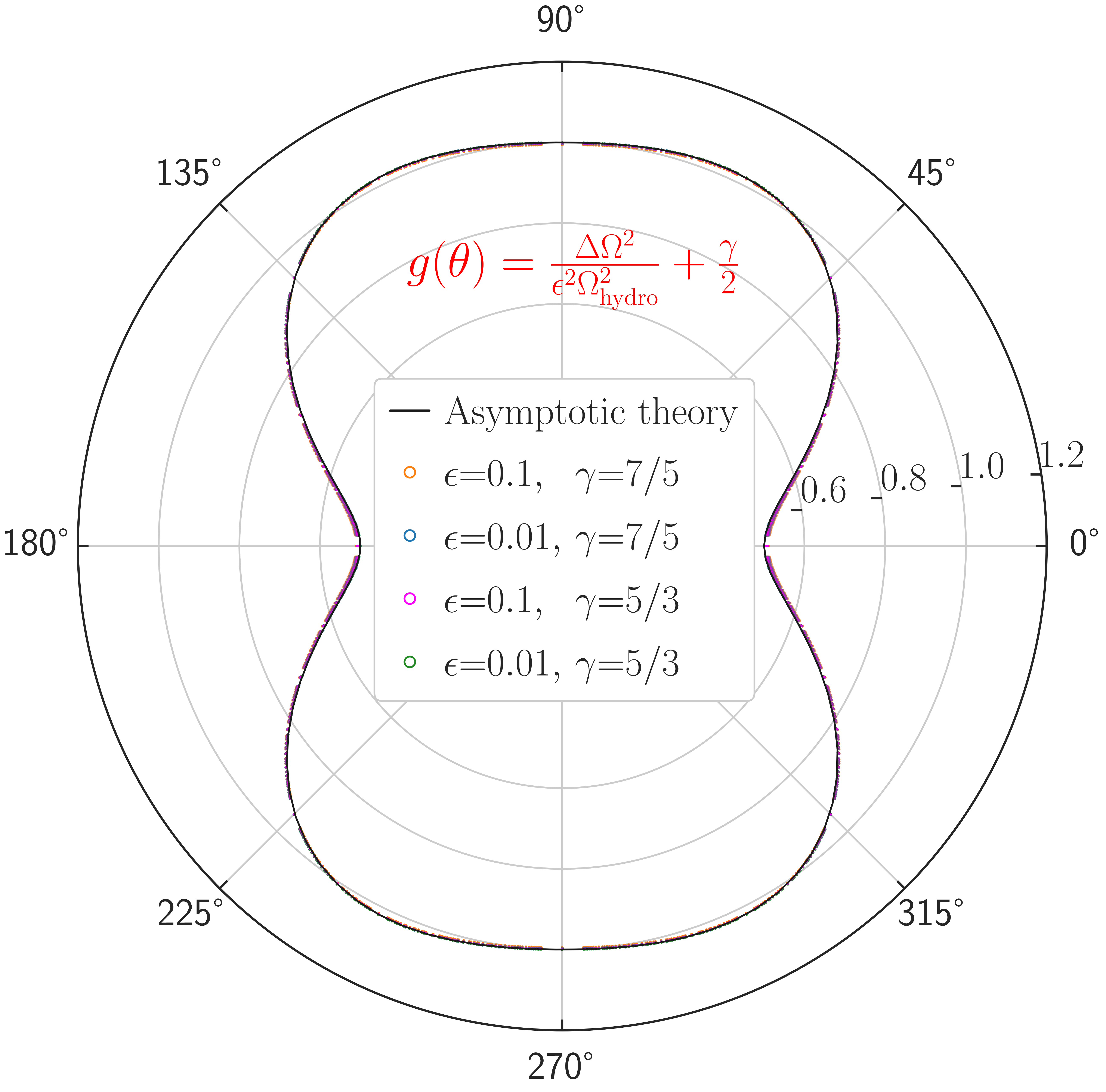
Figure 5: Theory and numerics: Our theory predicts that $g(\theta)=\Delta\Omega^{2}/({\mathbb{\color[rgb]{0,0,0}\epsilon}}^{2}\Omega_{\rm hydro}^{2})+\gamma/2$ depends only on $\theta$ as given in Eq. (41). The function $g(\theta)$ is independent of the wavenumber $K$, Alfvénic Mach number $\epsilon^{-1}$, the polytropic index $n$, the adiabatic index $\gamma$, and the eigen-state index $m$. Here, we plot $g(\theta)$ obtained from our numerical solutions for several different values of $m$, ranging from $10$ to $35$, and for several different values of $K$ ($0.6\leq|K|\leq 2$), and for two values of ${\mathbb{\color[rgb]{0,0,0}\epsilon}}$ and two values of $\gamma$ (different symbols). All data points collapse on the same universal curve. The function $g(\theta)$ from our asymptotic theory, Eq. (41), is also plotted here. The asymptotic curve is indistinguishable from the exact numerical solutions.

Using the Lamb’s relation, $\Omega_{\rm hydro}^{2}\sim K(2m+n)$, we rewrite Eq. (40) as

$$g(\theta) \equiv\gamma/2+\Delta\Omega^{2}/({\mathbb{\color[rgb]{0,0,0}\epsilon}}^{2}\Omega_{\rm hydro}^{2})$$ (41)

$$=1+\frac{1}{4}\left(\cos^{2}\theta-3\cos^{4}\theta\right),$$

where $\Delta\Omega^{2}\equiv\Omega^{2}-\Omega_{\rm hydro}^{2}$. This is a remarkable result. The right-hand-side of Eq. (41) is independent of every other possible parameter other than $\theta$ ! In Fig. 5, we plot the function $g(\theta)$ from our numerical determination of the eigenfrequencies for several different values of $m$ and $K$, and two different values of ${\mathbb{\color[rgb]{0,0,0}\epsilon}}$, and two different values of $\gamma$. These numerical values are shown as different symbols. All the different curves fall on top of each other, creating a universal curve. We also plot our asymptotic expression, Eq. (40), which agrees very well with the numerical results. This demonstrates that our theory is in excellent agreement with numerics even for ${\mathbb{\color[rgb]{0,0,0}\epsilon}}$ as large as ${\mathbb{\color[rgb]{0,0,0}\epsilon}}=0.1$.

It is surprising that, in our attempt to capture the anisotropy brought in by the magnetic field, despite a myriad of unwieldy expressions encountered on the way, an expression as simple as Eq. (40), is obtained. This simple expression is also highly accurate, as demonstrated in Fig. 5. The success of our asymptotic theory is somewhat unexpected, given that the analytical solution is accurate only up to the leading order ${\mathbb{\color[rgb]{0,0,0}\epsilon}}$ and $K/\Omega^{2}$.

More accurate solutions can be obtained by using the full expressions of $b_{0},b_{1},$ and $b_{2}$ from Appendix B in Eqs. (38d)–(38b), and keeping higher-order terms in ${\mathbb{\color[rgb]{0,0,0}\epsilon}}$ in Eq. (34).

Finally, a remark on the effect of magnetic fields on the slow gravity-driven waves is in order. For the slow waves, the first term on the left-hand side of Eq. (1) may be neglected, which implies that such waves in unmagnetized medium become unstable when $\gamma<(1+1/n)$. This is consistent with the energy principle of Newcomb (1961). When a magnetic field is present, by applying the energy principle of Newcomb, we find, for $K_{X}\neq 0$, the instability threshold on $\gamma$ for the gravity waves is lifted to $\gamma<(1+1/n)(1+1/\beta)$. When the magnetic field is very strong ($\beta\ll 1$), the regular perturbation series in powers of ${\mathbb{\color[rgb]{0,0,0}\epsilon}}\,(\propto 1/\sqrt{\beta})$ is possibly inadequate for unstable gravity-driven waves. Such considerations are clearly beyond the scope of the present paper.

6 Conclusions

Here we derive, for pressure-driven waves, an accurate and simple analytical formula that captures the effects of magnetic field and five other parameters: adiabatic index, polytropic index, eigenmode state index, wavenumbers, and the angle between the wavevector and the magnetic field [$\theta\mathrm{=}\cos^{-1}(\hat{\mathbf{K}}\cdot\hat{\bm{B}}_{0})$]. Such a six-parameter-dependent formula is distilled using a perturbative solution to magnetized version of Lamb’s hydrodynamic polytropic waves. Our explicit analytical formula overcomes the limitation of previously attempted formulae for the magnetized polytrope that were presented in general integral forms; such a formulation, for instance, that of Gough & Thompson [1990; e.g., Eq. (4.11)] and Bogdan & Cally (1997), requires numerical evaluation of the eigenfrequencies, and thus leaves out the critical step of obtaining an analytical understanding and expression. We achieve such here guided by our numerical solutions and at the cost of extensive use of Mathematica for our perturbative analyses.

We emphasize that the closed-form expression we obtain is not solely by use of perturbative calculation. At the last step, we needed guidance from our numerical solutions. A possible explanation for inadequacy of the perturbative calculation alone can be the ordering scheme in the perturbation series, which in this paper has two small parameters—one that corresponds to the WKB short-wavelength limit approximation and the other that is the actual small parameter, inverse of the Alfvénic Mach number. This implies that future work should develop better perturbation theory to take this inadequacy into account and to generalize our methodology to other complex wave problems.

The simplicity and accuracy of our formula are encouraging to employ the formula to help solve the inverse problem of magnetoseismology. Our formula provides an explicit, analytical dependence of the observed surface oscillation frequency with the orientation and strength of the deep-seated and subsurface magnetic field. Such an information can be crucial to predict the surface-emergence location and strength of sunspots. Precursors for such may be detected by analyzing the anisotropic magnetic effect in stellar ring diagrams—the rings of constant frequencies over the wavenumber plane.

Nonlinear asteroseismology can also directly benefit from our analytical work, as weak turbulence theory of asteroseismic waves inevitably requires accurate and simple expressions of linear wave frequencies in resonant triad interactions. The effect of the magnetic field on such is completely unknown. However, observations now exist that suggest resonant mode interactions are possible and can be a critical element of strongly pulsating stars (Guo, 2020). Nonlinear mode coupling of linear eigenmodes (Tripathi et al., 2023a, b) may also need to be analyzed, in addition to mode resonances. Future planned research will directly take advantage of the formula derived here to assess the role of the magnetic field and other parameters in asteroseismic wave turbulence, which is awaiting to soon enter adulthood from its infancy.

Data Availability

Mathematica notebook—built to perform lengthy analytical manipulations—and Dedalus script—used for numerical solution in this paper—are available at https://github.com/BindeshTripathi/polytrope.

Appendix A

The matrix elements $M_{ij}$ and $h_{\mu}$ that appear in Eq. (24) are

$$M_{11} =-\Omega^{2}(1+\gamma{\mathbb{\color[rgb]{0,0,0}\epsilon}}^{2}/2),$$ (A1a)

$$M_{12} =0,$$ (A1b)

$$M_{13} =\frac{-iK_{X}(n+1)(1+\gamma{\mathbb{\color[rgb]{0,0,0}\epsilon}}^{2}/2)}{\gamma},$$ (A1c)

$$M_{21} ={\mathbb{\color[rgb]{0,0,0}\epsilon}}^{2}K_{X}K_{Y}Z,$$ (A1d)

$$M_{22} =-\Omega^{2}(1+\gamma{\mathbb{\color[rgb]{0,0,0}\epsilon}}^{2}/2)+{\mathbb{\color[rgb]{0,0,0}\epsilon}}^{2}K_{X}^{2}Z,$$ (A1e)

$$M_{23} =\frac{-iK_{Y}(n+1)(1+\gamma{\mathbb{\color[rgb]{0,0,0}\epsilon}}^{2}/2)}{\gamma},$$ (A1f)

$$M_{31} =\frac{iK_{X}}{\gamma}\left[1+{\mathbb{\color[rgb]{0,0,0}\epsilon}}^{2}\left(\frac{3\gamma}{2}+\frac{K_{X}^{2}Z}{\Omega^{2}}\right)\right],$$ (A1g)

$$M_{32} =\frac{iK_{Y}}{\gamma}\left[1+{\mathbb{\color[rgb]{0,0,0}\epsilon}}^{2}\left(\frac{\gamma}{2}+\frac{K_{X}^{2}Z}{\Omega^{2}}\right)\right],$$ (A1h)

$$M_{33} =\frac{-\Omega^{2}(1+\gamma{\mathbb{\color[rgb]{0,0,0}\epsilon}}^{2}/2)+{\mathbb{\color[rgb]{0,0,0}\epsilon}}^{2}K_{X}^{2}Z}{n+1},$$ (A1i)

$$h_{x} =iK_{X}Z\hat{\chi},$$ (A1j)

$$h_{y} =iK_{Y}Z\hat{\chi}(1+{\mathbb{\color[rgb]{0,0,0}\epsilon}}^{2}),$$ (A1k)

$$h_{z} =\hat{\chi}+\frac{Z\partial_{Z}\hat{\chi}}{n+1}+{\mathbb{\color[rgb]{0,0,0}\epsilon}}^{2}\hat{\chi}\left[1+\frac{K_{X}^{2}Z\left\{\gamma-(n+1)(1+\gamma{\mathbb{\color[rgb]{0,0,0}\epsilon}}^{2}/2)\right\}}{(n+1)\gamma\Omega^{2}(1+\gamma{\mathbb{\color[rgb]{0,0,0}\epsilon}}^{2}/2)}\right]+{\mathbb{\color[rgb]{0,0,0}\epsilon}}^{2}\frac{Z\partial_{Z}\hat{\chi}}{n+1}\left[1+\frac{K_{X}^{2}Z}{\Omega^{2}(1+\gamma{\mathbb{\color[rgb]{0,0,0}\epsilon}}^{2}/2)}\right].$$ (A1l)

Appendix B

The parameters introduced in Eq. (31b), while writing the expression for $\Gamma_{2}(Z)$, appear below:

$$b_{2} =\frac{-K^{3}\cos^{4}\theta}{\Omega^{2}},$$ (A2a)

$$b_{1} =\frac{-K\left[-\Omega^{8}\gamma^{4}+\Omega^{4}\gamma^{2}K^{2}(n+1)\left\{(n+1+\gamma-\gamma n)\cos(2\theta)-n-1-3\gamma\right\}+2K^{4}(n+1)^{4}-K^{4}(n+1)^{3}(n+1-\gamma n)\cos(2\theta)\right]}{2\Omega^{4}\gamma^{2}\mathrm{sec}^{2}\theta\,\left[\Omega^{4}\gamma^{2}-K^{2}(n+1)^{2}\right]},$$ (A2b)

$$b_{0} =\frac{\Bigg{(}\begin{gathered}4\Omega^{8}\gamma^{4}(2-\gamma)-2\Omega^{4}\gamma^{2}K^{2}\left\{2(n+1)^{2}(4-3\gamma)+n(2n+3)\gamma^{2}\right\}+K^{4}(n+1)^{2}\left\{n\gamma^{2}(2n+3)-8(n+1)^{2}(\gamma-1)\right\}\\ +2K^{2}\gamma\cos(2\theta)\left[K^{2}(n+1)^{2}\left\{n(\gamma-4+2n(\gamma-1))-2\right\}+\Omega^{4}\gamma^{2}\left\{2(n+1)^{2}-\gamma n(2n+3)\right\}\right]+n\gamma^{2}K^{4}(n+1)^{2}\cos(4\theta)\end{gathered}\Bigg{)}}{16\Omega^{2}\gamma^{2}K\left[\Omega^{4}\gamma^{2}-K^{2}(n+1)^{2}\right]}$$ (A2e)

Appendix C

Due to the magnetic field, the locations of the turning points, $Z_{1}$ and $Z_{2}$, shift—which to the second order in ${\mathbb{\color[rgb]{0,0,0}\epsilon}}$ in Eq. (33) are given by $Z_{1}^{(2)}$ and $Z_{2}^{(2)}$:

$$Z_{1}^{(2)} =\frac{\alpha(b_{2}\alpha^{2}+b_{1}\alpha+b_{0})}{K(\beta-\alpha)},$$ (A3a)

$$Z_{2}^{(2)} =\frac{-\beta(b_{2}\beta^{2}+b_{1}\beta+b_{0})}{K(\beta-\alpha)}.$$ (A3b)

References

- Adam (1977) Adam, J. 1977, Solar Physics, 52, 293
- Aerts et al. (2010) Aerts, C., Christensen-Dalsgaard, J., & Kurtz, D. W. 2010, Asteroseismology (Springer Science & Business Media)
- Bender & Orszag (1978) Bender, C. M., & Orszag, S. A. 1978, Advanced Mathematical Methods for Scientists and Engineers
- Bogdan & Cally (1997) Bogdan, T. J., & Cally, P. S. 1997, Proceedings of the Royal Society of London Series A, 453, 943, doi: 10.1098/rspa.1997.0052
- Burns et al. (2020) Burns, K. J., Vasil, G. M., Oishi, J. S., Lecoanet, D., & Brown, B. P. 2020, Physical Review Research, 2, 023068, doi: 10.1103/PhysRevResearch.2.023068
- Cally (2007) Cally, P. S. 2007, Astronomische Nachrichten, 328, 286, doi: 10.1002/asna.200610731
- Cally & Bogdan (1997) Cally, P. S., & Bogdan, T. 1997, The Astrophysical Journal, 486, L67
- Campos (1983) Campos, L. 1983, Wave Motion, 5, 1
- Campos & Marta (2015) Campos, L., & Marta, A. 2015, Geophysical & Astrophysical Fluid Dynamics, 109, 168
- Chandrasekhar (1961) Chandrasekhar, S. 1961, Hydrodynamic and hydromagnetic stability, 652 pp., clarendon, Oxford, UK
- Das (2022) Das, S. B. 2022, The Astrophysical Journal, 940, 92
- Das et al. (2020) Das, S. B., Chakraborty, T., Hanasoge, S. M., & Tromp, J. 2020, The Astrophysical Journal, 897, 38
- Gough & Thompson (1990) Gough, D., & Thompson, M. 1990, Monthly Notices of the Royal Astronomical Society, 242, 25
- Guo (2020) Guo, Z. 2020, ApJ, 896, 161, doi: 10.3847/1538-4357/ab911f
- Hasselmann (1962) Hasselmann, K. 1962, Journal of Fluid Mechanics, 12, 481, doi: 10.1017/S0022112062000373
- Ilonidis et al. (2011) Ilonidis, S., Zhao, J., & Kosovichev, A. 2011, Science, 333, 993, doi: 10.1126/science.1206253
- Lamb (1911) Lamb, H. 1911, Proceedings of the Royal Society of London Series A, 84, 551, doi: 10.1098/rspa.1911.0008
- Nazarenko & Lukaschuk (2016) Nazarenko, S., & Lukaschuk, S. 2016, Annual Review of Condensed Matter Physics, 7, 61, doi: 10.1146/annurev-conmatphys-071715-102737
- Newcomb (1961) Newcomb, W. A. 1961, Physics of Fluids, 4, 391, doi: 10.1063/1.1706342
- Nye & Thomas (1976) Nye, A. H., & Thomas, J. H. 1976, ApJ, 204, 573, doi: 10.1086/154205
- Schunker et al. (2005) Schunker, H., Braun, D. C., Cally, P. S., & Lindsey, C. 2005, The Astrophysical Journal, 621, L149
- Singh et al. (2015) Singh, N. K., Brandenburg, A., Chitre, S., & Rheinhardt, M. 2015, Monthly Notices of the Royal Astronomical Society, 447, 3708
- Singh et al. (2014) Singh, N. K., Brandenburg, A., & Rheinhardt, M. 2014, The Astrophysical Journal Letters, 795, L8
- Singh et al. (2016) Singh, N. K., Raichur, H., & Brandenburg, A. 2016, The Astrophysical Journal, 832, 120
- Singh et al. (2020) Singh, N. K., Raichur, H., Käpylä, M. J., et al. 2020, Geophysical & Astrophysical Fluid Dynamics, 114, 196
- Thomas (1983) Thomas, J. H. 1983, Annual Review of Fluid Mechanics, 15, 321
- Tripathi (2022) Tripathi, B. 2022, Phys. Rev. D, 105, 036010, doi: 10.1103/PhysRevD.105.036010
- Tripathi et al. (2023a) Tripathi, B., Fraser, A. E., Terry, P. W., et al. 2023a, Physics of Plasmas, 30, 072107, doi: 10.1063/5.0156560
- Tripathi & Mitra (2022) Tripathi, B., & Mitra, D. 2022, ApJ, 934, 61, doi: 10.3847/1538-4357/ac79b1
- Tripathi et al. (2023b) Tripathi, B., Terry, P. W., Fraser, A. E., Zweibel, E. G., & Pueschel, M. J. 2023b, Physics of Fluids, 35, 105151, doi: 10.1063/5.0167092
- Van Beeck et al. (2021) Van Beeck, J., Bowman, D. M., Pedersen, M. G., et al. 2021, A&A, 655, A59, doi: 10.1051/0004-6361/202141572
- Van Beeck et al. (2023) Van Beeck, J., Van Hoolst, T., Aerts, C., & Fuller, J. 2023, arXiv e-prints, arXiv:2311.02972, doi: 10.48550/arXiv.2311.02972