Learning equilibria in Cournot mean field games of controls

Abstract

We consider Cournot mean field games of controls, a model originally developed for the production of an exhaustible resource by a continuum of producers. We prove uniqueness of the solution under general assumptions on the price function. Then, we prove convergence of a learning algorithm which gives existence of a solution to the mean field games system. The learning algorithm is implemented with a suitable finite difference discretization to get a numerical method to the solution. We supplement our theoretical analysis with several numerical examples and illustrate the impacts of model parameters.

1 Introduction

Mean field games (MFG) theory has been introduced in [29, 32] (see [12, 15] for a comprehensive introduction) as a tool to study games with infinitely many agents and it is particularly suitable to model economic problems for market competition. While in the first formulation of the theory the influence of the mass of agents on the single player occurs only through the spatial distribution, a subsequent development, known as mean field games of controls, considers the case in which the agent also reacts to decisions, i.e. optimal controls, of the other agents (see [10, 14, 19, 30]). In this latter framework, a very interesting problem, first proposed in [26, 27] and then widely studied in literature, is the one known as Cournot mean field games of controls, a model for the production of an exhaustible resource by a continuum of producers.

To introduce the Cournot model, we start describing the control problem solved by the representative agent. The state variable $x\in\mathbb{L}=(0,L)$ represents the inventory level. The dynamics of the agent, a producer, is given by the reflected stochastic differential equation

$$dX_{\tau}=-q_{\tau}\,d\tau+\sqrt{2\sigma^{2}(x)}dB_{\tau}-d\xi_{X_{\tau}},\,\,X_{t}=x,$$ (1)

where $d\xi_{X_{\tau}}$ is the local time at $x=L$ and $q_{\tau}=q(\tau,X_{\tau})$ is the control variable which gives the instantaneous rate of production. For $t\in(0,T)$, letting $\tau^{*}:=\inf\{\tau\geq t:\,\,X_{\tau}\leq 0\}$ the value function is

$$u(t,x)=\sup_{q_{\tau}\geq 0}{\mathbb{E}}\left\{\int_{t}^{T\wedge\tau^{*}}e^{-\lambda(\tau-t)}\Big{(}q_{\tau}\mathrm{P}(\tau)-\gamma q_{\tau}-\kappa q^{2}_{\tau}\Big{)}d\tau+e^{-\lambda({T\wedge\tau^{*}}-t)}u(X_{T\wedge\tau^{*}})\right\}.$$ (2)

where $\lambda>0$ is the discount factor, $\mathrm{P}(\tau)$ is the price, $\gamma q+\kappa q^{2}$, with $\gamma,\,\kappa>0$, the production cost. Given the function $m(t,\cdot)$ which describes the distribution of the agents at time $t$, assume that

• In equilibrium, all agents are using the same policy, which we denote by $\mathrm{q}(\tau,\cdot)$, but they are heterogeneous in their inventories $X_{\tau}$;

• Each agent is infinitesimally small, i.e. the producers influence the market price $\mathrm{P}(\tau)$ only through the average production $\int_{0}^{L}\mathrm{q}(\tau,x)m(\tau,x)dx$;

• Each agent is a price taker, taking as given the price $\mathrm{P}(\tau)$ from its “belief”, hence the $\sup$ in Eq. 2 is only over $q_{\tau}$.

Then, the Nash equilibria can be characterized by the MFG of controls system (cfr. [26, Proposition 3.1, p. 26]):

$$\left\{\begin{aligned} \textit{(i)}\qquad&\partial_{t}u+\sigma^{2}(x)\partial^{2}_{xx}u-\lambda u+\sup_{q\geq 0}\left\{-q\partial_{x}u+q\mathrm{P}(t)-\gamma q-\kappa q^{2}\right\}=0\qquad&&{\rm in}\,\,Q,\\ &\mathrm{P}(t)=P\Big{(}t,\int_{0}^{L}\mathrm{q}(t,x)m(t,x)dx\Big{)},u(t,0)=0,\,\partial_{x}u(t,L)=0&&{\rm in}\,[0,T],\\ &u(T,x)=u_{T}(x)&&{\rm in}\,\,\mathbb{L},\\ \textit{(ii)}\qquad&\partial_{t}m-\partial^{2}_{xx}\big{(}\sigma^{2}(x)m\big{)}-\text{div}(m\mathrm{q})=0&&{\rm in}\,\,Q,\\ &m(t,0)=0,\,\,\partial_{x}\big{(}\sigma^{2}(L)m(t,L)\big{)}+\mathrm{q}(t,L)m(t,L)=0&&{\rm in}\,[0,T],\\ &m(0,x)=m_{0}(x)&&{\rm in}\,\,\mathbb{L},\\ \textit{(iii)}\qquad&\mathrm{q}(t,x)=\arg\max_{q\geq 0}\left\{-q\partial_{x}u+q\mathrm{P}(t)-\gamma q-\kappa q^{2}\right\},\end{aligned}\right.$$ (3)

where $Q:=(0,T)\times\mathbb{L}$. $P(t,\cdot)$ is the price function. Eq. 3 (i) is the backward in time Hamilton-Jacobi-Bellman (HJB) equation characterizing the value function $u(t,x)$ for a representative agent (producer) at time $t$ and inventory state $x$; (ii) is a forward in time Fokker-Planck-Kolmogorov equation (FPK) which governs the evolution of the probability distribution $m(t)$ driven by the optimal control $\mathrm{q}(t,x)$; (iii) is a fixed point equation characterizing the optimal policy $\mathrm{q}(t,x)$ for the single producer at time $t$ and inventory level $x$. Note that the coupling term in (i) depends not only on the distribution of the agents $m(t,x)$, but also on the optimal rate of production $\mathrm{q}(t,x)$. This is a difficulty at the core of MFG of controls. The Cournot model in our paper has additional structure motivated by economic intuitions, making it more trackable than general MFG of controls.

Given the boundary conditions for $u$ and $m$ in the MFG system, the operator defining the FPK equation is the adjoint of the infinitesimal generator of the stochastic process Eq. 1, in the sense that,

$$\int_{0}^{L}\left(-\partial^{2}_{xx}\left(\sigma^{2}(x)m\right)-\text{div}(m\mathrm{q})\right)\phi dx=\int_{0}^{L}\left(-\sigma^{2}(x)\partial^{2}_{xx}u+\mathrm{q}\partial_{x}u\right)mdx\quad t\in[0,T].$$ (4)

From (i) and (iii) in system (3), the equation for the optimal policy can be reformulated more explicitly as

$$\mathrm{q}(t,x)=\left(\frac{P\big{(}t,\int_{0}^{L}\mathrm{q}(t,x)m(t,x)dx\big{)}-\gamma-\partial_{x}u(t,x)}{2\kappa}\right)_{+}.$$ (5)

Therefore $\mathrm{q}$ is characterized as a recursive competitive equilibrium.

Throughout the paper we will be also using the notation for the Hamiltonian:

$$H\left(\mathrm{P}\left(t\right)-\gamma-\partial_{x}u\right)=\sup_{q\geq 0}\left\{-q\partial_{x}u+q\mathrm{P}(t)-\gamma q-\kappa q^{2}\right\}.$$ (6)

We denote the flux at $(t,x)$ and aggregate production at $t$, respectively by:

$$\mathrm{w}(t,x)=\mathrm{q}(t,x)m(t,x),\,\,\,\psi(t)=\int_{0}^{L}\mathrm{w}(t,x)dx.$$ (7)

Following [26, 27], the price function $P$ is determined according to a rule of supply/demand equilibrium on the market, where the demand is given by a function $D(t,P)$, monotonically decreasing w.r.t. the $P$-variable. Hence for any aggregate production at time $t$, designated by $a\geq 0$,

$$D(t,P)=a,\,\,\,P\big{(}t,a\big{)}=D(t,\cdot)^{-1}(a).$$ (8)

and we recall from (3) (i) and $\psi(t)$ from Eq. 7 that $\mathrm{P}(t)=P\big{(}t,\psi(t)\big{)}=D(t,\cdot)^{-1}\big{(}\psi(t)\big{)}.$ Two typical examples of demand and price functions are given by (see [27]):

$$D(t,P)=Ee^{\rho t}(\pi_{\text{sub}}-P),\,\,P(t,a)=\pi_{\text{sub}}-\frac{1}{E}e^{-\rho t}a;$$ (9)

$$D(t,P)=Ee^{\rho t}P^{-\eta}-\delta,\,\,P(t,a)=E^{\frac{1}{\eta}}e^{\frac{\rho t}{\eta}}\frac{1}{\big{(}\delta+a\big{)}^{\frac{1}{\eta}}}.$$ (10)

In both of these examples, $E>0$ stands for a global wealth factor and $\rho$ for the growth of demand in the economy. In Eq. 9 the constant $\pi_{\text{sub}}>0$ is exogenous and represents the price of a substitute. The demand in Eq. 10 satisfies constant elasticity of substitution (CES), where a high $\delta$ stands for a low price of substitution.

The model previously described was proposed in [26, 27] and discussed also in [15]. Theoretical analysis was developed in [21, 23, 24, 22, 25], but mainly in the case of a linear price function. Even though nonlinear price functions have been considered by some of these works, they had different economic interpretations and assumptions, see Remark 2.3 for more details. Numerical simulations of Cournot MFG of controls have been considered in [27] and then in [16] and [35].

To our knowledge, there has not been a complete analysis of the model in [26, 27] for nonlinear price functions. Under natural assumptions on $P(t,\cdot)$, which in particular include the ones defined in Eqs. 9 and 10, we prove existence and uniqueness of the classical solution to system (3). Existence is obtained by proving the global convergence of the smoothed policy iteration (SPI) algorithm, an iterative learning procedure introduced in [37] for solving MFG systems. This method is similar to fictitious play (see [13] and [35]) as a learning algorithm, but the agent only evaluates a policy (which amounts to solving a linear problem) and then performs a greedy update. The convergence analysis of (SPI) for Cournot MFG of controls, even though highly based on the theoretical apparatus developed in [37], faces essential difficulties and contains differences due to the recursive characterization of the optimal policy, see (iii) in system (3). To our knowledge there has not been theoretical convergence analysis of iterative algorithms in this general setting for Cournot MFG of controls.

Dealing with the numerical resolution of MFG systems by finite difference method typically requires using some iterative algorithms, e.g. fixed point [3, 5], Newton method [2, 1], fictitious play [13, 28, 33, 35], policy iteration [8, 11, 34] or smoothed policy iteration [37]. See e.g. [4, 33] and the references therein for more details. In particular, [35] considered convergence rate of a fictitious play algorithm for solving an MFG of controls, similar to our Cournot model but with only linear price function and periodic boundary conditions. [3] considered numerical solution of a Cucker-Smale type MFG of controls with periodic or Neumann boundary conditions. Fictitious play type iterative computation has been considered in [18, 38] for one shot Cournot games with a finite number of agents. Based on a finite difference discretization of (SPI), we define an efficient numerical method for the resolution of system (3). While developing the numerical scheme, special attention is paid to preserving the adjoint structure of the MFG system and to the consistency of the flux boundary condition for the FPK equation.

We observe that, in contrast to [27] where the Cournot MFG of controls was considered on the interval $[0,T]\times[0,+\infty)$, we study the problem on the bounded interval $[0,T]\times[0,L]$ and we impose a Neumann boundary condition for $u$ and the dual flux boundary condition for $m$ at $x=L$. Moreover in [27], the dynamics of the agent is given by a geometric Brownian motion (GBM), hence the diffusion coefficient $\sigma^{2}(x)$ may degenerate at $x=0$. We assume $\sigma>0$ in the theoretical analysis. However, our numerical experiments show that the method performs well in models with GBM diffusions. We plan to consider the theoretical aspects of the degenerate diffusion in the future. We conclude observing that our analytical and numerical method can be extended to consider a wide range of competitive equilibrium models.

2 Assumptions and preliminary results

We first introduce some functional spaces. For any $\mathrm{r}\geq 1$, $L^{\mathrm{r}}(\mathbb{L})$ and $L^{\mathrm{r}}(Q)$ are the usual Lebesgue spaces. Given a Banach space $X$, $L^{\mathrm{r}}(0,T;X)$ is the vector-valued Lebesgue spaces. We denote with $H^{1}(\mathbb{L})$ the space of all functions $\mathrm{u}$ on $\mathbb{L}$, such that $\mathrm{u}(0)=0$ and the norm

$$\|\mathrm{u}\|_{H^{1}(\mathbb{L})}:=\|\mathrm{u}\|_{L^{2}(\mathbb{L})}+\|\partial_{x}\mathrm{u}\|_{L^{2}(\mathbb{L})}$$

is finite. The dual space of $H^{1}(\mathbb{L})$ is denoted by $H^{-1}(\mathbb{L})$. We denote by $W^{1,2}_{\mathrm{r}}(Q)$ the space of functions $u$ such that $u,\partial_{t}u,\partial_{x}u,\partial^{2}_{xx}u$ are all in $L^{\mathrm{r}}(Q)$, endowed with the norm

$$\|u\|_{W^{1,2}_{\mathrm{r}}(Q)}:=\|u\|_{L^{\mathrm{r}}(Q)}+\|\partial_{t}u\|_{L^{\mathrm{r}}(Q)}+\|\partial_{x}u\|_{L^{\mathrm{r}}(Q)}+\|\partial^{2}_{xx}u\|_{L^{\mathrm{r}}(Q)}.$$

We also denote by $V^{0,1}_{2}(Q)$ the Banach space of function $u:Q\rightarrow\mathbb{R}$ such that the norm (cfr. [31] p.6)

$$\|u\|_{V^{0,1}_{2}(Q)}:=\max_{0\leq t\leq T}\|u(t,\cdot)\|_{L^{2}(\mathbb{L})}+\|\partial_{x}u\|_{L^{2}(Q)}.$$

Let $\mathcal{C}^{0}(Q)$ be the space of continuous functions in $Q$ and $\mathcal{C}^{0,1}(Q)$ the space of functions in $\mathcal{C}^{0}(Q)$ and once continuously differentiable w.r.t. $x$. For $\alpha\in(0,1)$, $\mathcal{C}^{\alpha/2,\alpha}(Q)$ and $\mathcal{C}^{1+\alpha/2,2+\alpha}(Q)$ denote the spaces of Hölder continuous functions in $Q$, endowed with the norms

$$\|u\|_{\mathcal{C}^{\alpha/2,\alpha}(Q)}:=\|u\|_{\mathcal{C}^{0}(Q)}+\sup_{(t_{1},x_{1})\neq(t_{2},x_{2})\in Q}\frac{|u(t_{1},x_{1})-u(t_{2},x_{2})|}{\big{(}|x_{1}-x_{2}|^{2}+|t_{1}-t_{2}|\big{)}^{\alpha/2}},$$ (11)

$$\|u\|_{\mathcal{C}^{(1+\alpha)/2,1+\alpha}(Q)}:=\|u\|_{\mathcal{C}^{0}(Q)}+\|\frac{\partial u}{\partial x}\|_{\mathcal{C}^{\alpha/2,\alpha}(Q)}+\sup_{(t_{1},x)\neq(t_{2},x)\in Q}\frac{|u(t_{1},x)-u(t_{2},x)|}{|t_{1}-t_{2}|^{(1+\alpha)/2}},$$ (12)

$$\|u\|_{\mathcal{C}^{1+\alpha/2,2+\alpha}(Q)}:=\|u\|_{\mathcal{C}^{0}(Q)}+\|\frac{\partial u}{\partial x}\|_{\mathcal{C}^{(1+\alpha)/2,1+\alpha}(Q)}+\|\frac{\partial u}{\partial t}\|_{\mathcal{C}^{\alpha/2,\alpha}(Q)}.$$ (13)

As we will make strong assumptions on the regularity of the initial and boundary conditions, we only need Sobolev spaces with $r\geq 3$. Throughout the paper we use $r$ for an arbitrary constant such that $r\geq 3$. It is know from [31, Corollary pp. 342-343] that

$$W^{1,2}_{r}(Q)\,\,\text{is compactly embedded in}\,\,\mathcal{C}^{(1+\alpha)/2,1+\alpha}(Q)\quad\forall\alpha\in(0,1).$$ (14)

We make the following standing assumptions:

Assumption 2.1.

We assume:

1. $m_{0}$ is $\mathcal{C}^{3}(\mathbb{L})$, $\int_{0}^{L}m_{0}(x)dx=1$, $m_{0}(x)\geq 0$ and $m_{0}(0)=0$.

2. $u_{T}$ is $\mathcal{C}^{3}(\mathbb{L})$ and

   $$\partial_{x}u_{T}(x)\geq 0,\,u_{T}(0)=0,\,\partial_{x}u_{T}(L)=0.$$

3. The price function $P(t,a):[0,T]\times\mathbb{R}^{+}\rightarrow\mathbb{R}$ is $\mathcal{C}^{2}$ for both variables. $\partial_{a}P(t,a)\leq 0$ for all $t\in[0,T]$. There exists $\Phi(t,a):[0,T]\times\mathbb{R}^{+}\rightarrow\mathbb{R}$, $\Phi$ being $\mathcal{C}^{3}$ for both variables, such that $P(t,a)=\partial_{a}\Phi(t,a)$ for all $t\in[0,T]$. Moreover, there exist $C_{P}>0$, such that

   $$\gamma<P(t,0)\leq C_{P}+\gamma,\quad\forall t\in[0,T].$$

4. The viscosity coefficient $\sigma(\cdot)$ is $\mathcal{C}^{2}(\mathbb{L})$ and non degenerate, i.e. $\sigma(x)\geq\sigma_{0}>0$.

Remark 2.2.

(A2.1.3) implies

$$P(t,a)\leq C_{P}+\gamma,\quad\forall t\in[0,T].$$ (15)

We observe that (A2.1.3) is satisfied by both examples Eq. 9 and Eq. 10, by setting $C_{P}=\pi_{\text{sub}}-\gamma$ in Eq. 9 and $C_{P}=(\frac{E}{\delta})^{\frac{1}{\eta}}-\gamma$ in Eq. 10. Moreover, in both the case the price $\mathrm{P}$ can be derived from a potential $\Phi$ by setting in Eq. 9

$$\Phi\big{(}t,\psi(t)\big{)}=\pi_{\text{sub}}\psi(t)-\frac{1}{2E}e^{-\rho t}\big{(}\psi(t)\big{)}^{2},$$

and in Eq. 10

$$\Phi(t,\psi(t))=\left\{\begin{aligned} \qquad&\frac{E^{\frac{1}{\eta}}e^{\frac{\rho t}{\eta}}}{1-\frac{1}{\eta}}\big{(}\delta+\psi(t)\big{)}^{1-\frac{1}{\eta}},\qquad&&\text{if}\,\,\eta>1,\\ \qquad&Ee^{\rho t}\ln\big{(}\delta+\psi(t)\big{)},&&\text{if}\,\,\eta=1.\end{aligned}\right.$$

Remark 2.3.

We now consider a particular case of the linear price impact model Eq. 9 by taking $\rho=\gamma=0$ and $\kappa=1$. The revenue of the producer (income minus cost) then becomes:

$$q\mathrm{P}(t)-\gamma q-\kappa q^{2}=q(\pi_{\text{sub}}-\frac{1}{E}\psi(t)-q).$$

If we interpret $\frac{1}{E}$ as the measure of competition between producers and $\tilde{P}(t)=\pi_{\text{sub}}-\frac{1}{E}\psi(t)-q$ as the price, then we recover the price impact model in literature [24, 21, 23, 22, 25]. Generalizations, e.g. in [25], consist in price of the form

$$\tilde{P}(t)=\pi_{\text{sub}}-\Psi\big{(}\frac{1}{E}\psi(t)+q\big{)},$$ (16)

where $\Psi$ is a nonlinear monotone increasing function. A typical condition for the existence and uniqueness of solution to the Cournot MFG system with price defined by Eq. 16 is the smallness of $\frac{1}{E}$ or $T$. Smallness conditions for general MFG of controls model have been discussed in [10, 30]. In our model, following [27], we assume that the price depends only on the average production $\psi(t)$ and we make no smallness assumptions on the parameters throughout the paper.

We first consider some results related to the FPK equation with Robin boundary conditions (see [5, 7, 17] for related results). Given the initial-boundary value problem

$$\left\{\begin{aligned} \qquad&\partial_{t}m-\partial^{2}_{xx}(\sigma^{2}(x)m)-{\rm{div}}(mq)=0\qquad&&{\rm in}\,Q,\\ \qquad&m(t,0)=0\,\,\text{and}\,\,\partial_{x}\big{(}\sigma^{2}(L)m(t,L)\big{)}+m(t,L)q(t,L)=0&&{\rm in}\,[0,T],\\ \qquad&m(0,x)=m_{0}(x)&&{\rm in}\,\mathbb{L}.\end{aligned}\right.$$ (17)

We give the following definition of weak solution (see [31, Chapter V, section 1]).

Definition 2.4.

A function $m$ is said to be a bounded weak solution to Eq. 17 if $m\in L^{\infty}(Q)$, $\partial_{x}m\in L^{2}(Q)$ and

$$\int_{0}^{L}m(t,x)\varphi(t,x)dx-\int_{0}^{L}m_{0}(x)\varphi(0,x)dx+\int_{0}^{t}\int_{0}^{L}\left(-m\partial_{t}\varphi+\partial_{x}\varphi\partial_{x}\big{(}\sigma^{2}(x)m\big{)}+qm\partial_{x}\varphi\right)dxdt=0,$$

for any $t\in(0,T]$ and any function $\varphi$ such that $\varphi$, $\partial_{t}\varphi,\partial_{x}\varphi\in L^{2}(Q)$, $\varphi(t,0)=\varphi(t,L)=0$.

Lemma 2.5.

Suppose $m_{0}$ satisfies (A2.1.1) and $0\leq q(t,x)\leq R$. Then, there exists a unique solution $m$ to Eq. 17 satisfying $m\in L^{2}(0,T;H^{1}(\mathbb{L}))\cap L^{\infty}(Q)$, $\partial_{t}m\in L^{2}\big{(}0,T;H^{-1}(\mathbb{L})\big{)}$. In addition, $\|m\|_{C^{\alpha/2,\alpha}}(Q)\leq C$, $m(t,x)>0$ for all $t\in[0,T]$. Let $m_{\iota}$, $\iota=\{1,2\}$, be the solution to Eq. 17 corresponding to $q_{\iota}$ and set $\varrho=m_{1}-m_{2}$. Then

$$\|\varrho\|_{L^{\infty}(0,T;L^{2}(\mathbb{L}))}\leq C_{\varrho}\int_{0}^{L}m_{1}|q_{1}-q_{2}|^{2}dx,$$

where $C_{\varrho}$ is a constant depending only on $m_{0}$, $T$, $L$ and $R$.

Proof.

The existence and uniqueness of a weak solution

$$m\in L^{2}(0,T;H^{1}(\mathbb{L})),\,\,\,\partial_{t}m\in L^{2}\big{(}0,T;H^{-1}(\mathbb{L})\big{)}$$

is standard from energy estimates (cfr. [11]). From [7, Proposition 2.2], there exists a constant $C_{m}$ which depends only on $m_{0}$, $L$, $T$ and $R$ such that

$$\|m\|_{L^{\infty}(Q)}\leq C_{m}.$$

Therefore, $m$ is a bounded weak solution in the sense of Definition 2.4 and $\|m\|_{C^{\alpha/2,\alpha}(Q)}\leq C$ follows from [31, Chapter V, Theorem 1.1]. One can use duality method to show $m(t,x)\geq 0$ as in [20, Proposition 4.3], while $m(t,x)>0$ in $Q$ follows from (A2.1.1) and Harnack inequality (cf. [36, Theorem 6.27]) and [5, Proof of Theorem 2.2]. It is clear that $\varrho=m_{1}-m_{2}$ satisfies

$$\left\{\begin{aligned} \qquad&\partial_{t}\varrho-\partial^{2}_{xx}\big{(}\sigma^{2}(x)\varrho\big{)}-{\rm{div}}(\varrho q_{2})={\rm{div}}(m_{1}(q_{1}-q_{2})).\qquad&&{\rm in}\,Q,\\ \qquad&\varrho(t,0)=0,\,\partial_{x}\big{(}\sigma^{2}(L)\varrho(t,L)\big{)}+\varrho(t,L)q_{2}(t,L)+m_{1}(t,L)(q_{1}(t,L)-q_{2}(t,L))=0,\\ \qquad&\varrho(0,x)=0&&{\rm in}\,\mathbb{L}.\end{aligned}\right.$$

Then, by standard energy estimates (cfr. [11]), we obtain the result. ∎

Corollary 2.6.

Under the assumptions of Lemma 2.5, for all $0\leq t_{0}<t_{1}\leq T$, $\int_{0}^{L}m(t_{1},x)dx\leq\int_{0}^{L}m(t_{0},x)dx$.

Proof.

Since $\sigma^{2}(0)m(t,0)=0$ and $\sigma^{2}(x)m(t,x)\geq 0$ for all $x\in(0,L]$, then $\partial_{x}\big{(}\sigma^{2}(0)m(t,0)\big{)}\geq 0$. Integrating on $[t_{0},t_{1}]\times[0,L]$ the FPK equation

$$\partial_{t}m=\partial_{x}\big{(}\partial_{x}(\sigma^{2}(x)m)+qm\big{)}.$$

Using the boundary conditions $m(t,0)=0$, and $\partial_{x}\big{(}\sigma^{2}(L)m(t,L)\big{)}+q(t,L)m(t,L)=0$, we obtain

$$\int_{0}^{L}m(t_{1},x)dx-\int_{0}^{L}m(t_{0},x)dx=-\int_{t_{0}}^{t_{1}}\partial_{x}\big{(}\sigma^{2}(0)m(t,0)\big{)}dt\leq 0.$$

We now consider some preliminary results for the MFG system (3). Define the space

$$\mathbbm{X}:=\left\{(u,m,\mathrm{q}):\,\,u\in W^{1,2}_{r}(Q),m\in L^{2}(0,T;H^{1}(\mathbb{L}))\cap L^{\infty}(Q),\partial_{t}m\in L^{2}\big{(}0,T;H^{-1}(\mathbb{L})\big{)},\mathrm{q}\in L^{\infty}(Q)\right\},$$ (18)

we call a triple $(u,m,\mathrm{q})\in\mathbbm{X}$ a weak solution to the Cournot MFG of controls system (3) if (i) and (ii) are satisfied in the sense of distributions and (iii) is satisfied pointwise. ∎

Lemma 2.7.

Suppose $(u,m,\mathrm{q})$ is a weak solution to system (3). Then $u(t,x)\geq 0$ and $\partial_{x}u(t,x)\geq 0$. In addition,

$$0\leq\mathrm{q}(t,x)\leq\frac{C_{P}}{2\kappa},\quad\forall(t,x)\in Q,$$ (19)

$$\mathrm{P}(t)>\gamma,\quad\forall t\in[0,T].$$ (20)

Proof.

It is clear from (A2.1.2) that $u_{T}(x)\geq 0$ for all $x\in[0,L]$. From the HJB equation in system (3) obviously

$$\sup_{q\geq 0}\Big{\{}-q\partial_{x}u+q\mathrm{P}(t)-\gamma q-\kappa q^{2}\Big{\}}\geq 0,$$

hence

$$-\partial_{t}u-\sigma^{2}(x)\partial^{2}_{xx}u+\lambda u\geq 0.$$

The weak parabolic maximum principle implies that $u(t,x)\geq 0$. Since $u(t,0)=0$ for all $t$ we obtain $\partial_{x}u(t,0)\geq 0$ for all $t$. From Eq. 20, $\mathrm{P}\left(t\right)-\gamma\leq C_{P}$. Recall that $(\cdot)_{+}$ is a convex function, hence the Hamiltonian

$$H\left(\mathrm{P}\left(t\right)-\gamma-\partial_{x}u\right)=\kappa\left(\frac{\mathrm{P}\left(t\right)-\gamma-\partial_{x}u}{2\kappa}\right)_{+}^{2}\leq\frac{1}{\kappa}\left(\frac{(\mathrm{P}\left(t\right)-\gamma)_{+}+(-\partial_{x}u)_{+}}{2}\right)^{2}\leq\frac{C_{P}^{2}+(\partial_{x}u)^{2}}{2\kappa}.$$

It follows from standard estimates for quasilinear parabolic equations, e.g. [31, Chapter 5, Theorem 6.3], that $\partial_{x}u\in L^{\infty}(Q)$ and $u\in W^{1,2}_{r}(Q)$. The derivative of $H\left(\mathrm{P}\left(t\right)-\gamma-\partial_{x}u\right)$ w.r.t $x$ in the sense of distributions is

$$\left(\frac{\mathrm{P}\left(t\right)-\gamma-\partial_{x}u}{2\kappa}\right)_{+}\mathbf{1}_{\{\mathrm{P}\left(t\right)-\gamma-\partial_{x}u\geq 0\}}(-\partial_{xx}^{2}u),$$

where $\mathbf{1}_{\{\mathrm{P}\left(t\right)-\gamma-\partial_{x}u\geq 0\}}$ denotes an indicator function. We can differentiate the HJB equation (3) (i), with $\phi=\partial_{x}u$ being a weak solution to

$$\partial_{t}\phi+\sigma^{2}(x)\partial_{xx}^{2}\phi+2\sigma^{2}(x)\sigma^{\prime}(x)\partial_{x}\phi-\lambda\phi-\left(\frac{\mathrm{P}\left(t\right)-\gamma-\phi}{2\kappa}\right)_{+}\mathbf{1}_{\{\mathrm{P}\left(t\right)-\gamma-\phi\geq 0\}}\partial_{x}\phi=0.$$

From $\partial_{x}u\in L^{\infty}(Q)$, it is clear that $-\left(\frac{\mathrm{P}\left(t\right)-\gamma-\phi}{2\kappa}\right)_{+}\mathbf{1}_{\{\mathrm{P}\left(t\right)-\gamma-\phi\geq 0\}}$ is bounded in $L^{\infty}(Q)$. It is easy to see from $u\in W^{1,2}_{r}(Q)$ (or by using energy estimates) that $\phi\in V^{0,1}_{2}(Q)$. From $\phi(T,x)\geq 0$, $\phi(t,L)=0$ and $\phi(t,0)\geq 0$, we can use the parabolic maximum principle for weak solutions (cfr. [31, Chapter 3, Theorem 7.2, p. 188]) and obtain $\phi(t,x)\geq 0$ for all $(t,x)\in Q$. From $\partial_{x}u(t,x)\geq 0$ and Eq. 5 we obtain Eq. 19.

Next, we show Eq. 20 by a contradiction argument. Suppose $\mathrm{P}(\check{t})\leq\gamma$ at some time $\check{t}$. Then from $\partial_{x}u(\check{t},x)\geq 0$ we have

$$\mathrm{P}(\check{t})-\gamma-\partial_{x}u(\check{t},x)\leq 0.$$

With Eq. 5, we can then obtain $\mathrm{q}(\check{t},x)=0$ for all $x\in[0,L]$. This implies

$$P(\check{t},0)=P\left(\check{t},\int_{0}^{L}\mathrm{q}(\check{t},x)m(\check{t},x)dx\right)=\mathrm{P}(\check{t})\leq\gamma.$$

This is a contradiction as we have assumed $P(t,0)>\gamma$ for all $t\in[0,T]$ in (A2.1.3). ∎

Remark 2.8.

From an economic modeling point of view, Lemma 2.7 shows that the price $\mathrm{P}(t)$ will never be lower than $\gamma$, otherwise the optimal production of each producer will be $0$ and we have a contradiction.

It is clear that for $(t,x)$ such that $\mathrm{q}(t,x)>0$,

$$\partial_{x}u(t,x)=\mathrm{P}(t)-\frac{d\left(\gamma\mathrm{q}+\kappa\mathrm{q}^{2}\right)}{d\mathrm{q}}.$$

In other words, $\partial_{x}u$ equals the price minus the marginal production cost. Therefore, $\partial_{x}u$ can be interpreted as the Hotelling rent in [27], an index widely used for measuring scarcity of resources in the economic literature. Hence, another feature of the model is that the Hotelling rent is non negative.

Remark 2.9.

From Lemma 2.7, we can in fact replace the constraint $q\geq 0$ in (3) (i) and (iii) by $0\leq q\leq\frac{C_{P}}{2\kappa}$, i.e.

$$\mathrm{q}=\arg\max_{0\leq q\leq\frac{C_{P}}{2\kappa}}\left\{-q\partial_{x}u+q\mathrm{P}(t)-\gamma q-\kappa q^{2}\right\}.$$

This implies that the Hamiltonian is globally Lipschitz and therefore allows us to avoid using Bernstein estimates as in [30].

The following result is crucial for proving uniqueness of the solution to system (3) and convergence of learning algorithms. It is analogous to [13, Lemma 2.7] and [37, Lemma 2.8]. Here, since the admissible set of controls $q$ is compact( cf. Remark 2.9) we give a modified proof. The novelty in the proof is that we consider separately the case when the constraints on $q$ are binding.

Lemma 2.10.

Let $\Lambda\in\mathbb{R}$,

$$H(\Lambda)=\sup_{0\leq q\leq\frac{C_{P}}{2\kappa}}\left\{-q\Lambda-\kappa q^{2}\right\},\,\,\,\mathrm{q}=\arg\max_{0\leq q\leq\frac{C_{P}}{2\kappa}}\left\{-q\Lambda-\kappa q^{2}\right\},$$

then for all $q$ such that $0\leq q\leq\frac{C_{P}}{2\kappa}$,

$$H(\Lambda)-\Big{(}-q\Lambda-\kappa q^{2}\Big{)}\geq\kappa|\mathrm{q}-q|^{2}.$$ (21)

Proof.

We have:

$$H(\Lambda)-\Big{(}-q\Lambda-\kappa q^{2}\Big{)}=\kappa q^{2}-\kappa\mathrm{q}^{2}-\big{(}-\Lambda(q-\mathrm{q})\big{)}.$$

If $-C_{P}\leq\Lambda\leq 0$, then $\mathrm{q}=-\frac{\Lambda}{2\kappa}$, hence Eq. 21. If $\Lambda>0$, then $\mathrm{q}=0$,

$$H(\Lambda)-\Big{(}-q\Lambda-\kappa q^{2}\Big{)}=\kappa q^{2}+\Lambda q\geq\kappa|0-q|^{2}.$$

If $\Lambda<-C_{P}$, then $\mathrm{q}=\frac{C_{P}}{2\kappa}$ and $q-\mathrm{q}\leq 0$, hence $-\Lambda(\frac{C_{P}}{2\kappa}-q)\geq C_{P}(\frac{C_{P}}{2\kappa}-q)$,

$$H(\Lambda)=-\mathrm{q}\Lambda-\kappa\mathrm{q}^{2}=-\Lambda\frac{C_{P}}{2\kappa}-\kappa\left(\frac{C_{P}}{2\kappa}\right)^{2}.$$

Therefore,

$$H(\Lambda)-\Big{(}-q\Lambda-\kappa q^{2}\Big{)}=-\Lambda(\frac{C_{P}}{2\kappa}-q)+\kappa q^{2}-\kappa\left(\frac{C_{P}}{2\kappa}\right)^{2}\geq C_{P}(\frac{C_{P}}{2\kappa}-q)+\kappa q^{2}-\kappa\left(\frac{C_{P}}{2\kappa}\right)^{2}=\kappa|\frac{C_{P}}{2\kappa}-q|^{2}.$$

∎

3 Uniqueness of the solution

In this section, we prove uniqueness of the solution to system (3).

Theorem 3.1.

Under assumptions (A2.1.1), (A2.1.2) and (A2.1.3), system (3) has at most one weak solution $(u,m,\mathrm{q})\in\mathbbm{X}$.

Proof.

Suppose there exist two solutions $(u_{1},m_{1},\mathrm{q}_{1})$, $(u_{2},m_{2},\mathrm{q}_{2})$. Let $v=u_{1}-u_{2}$, $\varrho=m_{1}-m_{2}$. For $\iota\in\{1,2\}$, we set $\mathrm{w}_{\iota}=\mathrm{q}_{\iota}m_{\iota}$ and $\mathrm{P}_{\iota}(t)=P\big{(}t,\int_{0}^{L}\mathrm{w}_{\iota}dx\big{)}$. Hence

$$H\big{(}\partial_{x}u_{\iota}-\mathrm{P}_{\iota}(t)+\gamma\big{)}=\sup_{q\geq 0}\left\{-q\partial_{x}u_{\iota}+q\mathrm{P}_{\iota}(t)-\gamma q-\kappa q^{2}\right\}=-\mathrm{q}_{\iota}\partial_{x}u_{\iota}+\mathrm{q}_{\iota}\mathrm{P}_{\iota}(t)-\gamma\mathrm{q}_{\iota}-\kappa\mathrm{q}_{\iota}^{2}.$$

By comparing (i) and (ii) in the systems for $(u_{1},m_{1},\mathrm{q}_{1})$ and $(u_{2},m_{2},\mathrm{q}_{2})$, we get

$$\partial_{t}v+\sigma^{2}(x)\partial^{2}_{xx}v-\lambda v+H\big{(}\partial_{x}u_{1}-\mathrm{P}_{1}(t)+\gamma\big{)}-H\big{(}\partial_{x}u_{2}-\mathrm{P}_{2}(t)+\gamma\big{)}=0,$$

$$\partial_{t}\varrho-\partial^{2}_{xx}\big{(}\sigma^{2}(x)\varrho\big{)}-\partial_{x}(\mathrm{w}_{1}-\mathrm{w}_{2})=0.$$

Multiplying the previous equations by $e^{-\lambda t}\varrho$ and $e^{-\lambda t}v$ respectively, adding the resulting equations and integrating over $Q$, we get

$$0={} \int_{Q}e^{-\lambda t}\varrho\Big{(}\partial_{t}v+\sigma^{2}(x)\partial^{2}_{xx}v-\lambda v+H\big{(}\partial_{x}u_{1}-\mathrm{P}_{1}(t)+\gamma\big{)}-H\big{(}\partial_{x}u_{2}-\mathrm{P}_{2}(t)+\gamma\big{)}\Big{)}dxdt$$

$$+\int_{Q}e^{-\lambda t}v\Big{(}\partial_{t}\varrho-\partial^{2}_{xx}\big{(}\sigma^{2}(x)\varrho\big{)}-\partial_{x}(\mathrm{w}_{1}-\mathrm{w}_{2})\Big{)}dxdt.$$

Integrating by parts, we obtain

$$0={} -\int_{Q}e^{-\lambda t}m_{1}\Big{(}H\big{(}\partial_{x}u_{2}-\mathrm{P}_{2}(t)+\gamma\big{)}-H\big{(}\partial_{x}u_{1}-\mathrm{P}_{1}(t)+\gamma\big{)}-\mathrm{q}_{1}(\partial_{x}u_{1}-\partial_{x}u_{2})\Big{)}dxdt$$ (22)

$$-\int_{Q}e^{-\lambda t}m_{2}\Big{(}H\big{(}\partial_{x}u_{1}-\mathrm{P}_{1}(t)+\gamma\big{)}-H\big{(}\partial_{x}u_{2}-\mathrm{P}_{2}(t)+\gamma\big{)}-\mathrm{q}_{2}(\partial_{x}u_{2}-\partial_{x}u_{1})\Big{)}dxdt.$$

Since

$$H\big{(}\partial_{x}u_{1}-\mathrm{P}_{1}(t)+\gamma\big{)}+\mathrm{q}_{1}(\partial_{x}u_{1}-\partial_{x}u_{2})={} -\mathrm{q}_{1}\big{(}\partial_{x}u_{2}-\mathrm{P}_{1}(t)+\gamma\big{)}-\kappa\mathrm{q}_{1}^{2}$$

$$={} -\mathrm{q}_{1}\big{(}\partial_{x}u_{2}-\mathrm{P}_{2}(t)+\gamma\big{)}-\kappa\mathrm{q}_{1}^{2}+\mathrm{q}_{1}\big{(}\mathrm{P}_{1}(t)-\mathrm{P}_{2}(t)\big{)},$$

we have

$$\int_{Q}e^{-\lambda t}m_{1}\Big{(}H\big{(}\partial_{x}u_{2}-\mathrm{P}_{2}(t)+\gamma\big{)}-H\big{(}\partial_{x}u_{1}-\mathrm{P}_{1}(t)+\gamma\big{)}-\mathrm{q}_{1}(\partial_{x}u_{1}-\partial_{x}u_{2})\Big{)}dxdt$$ (23)

$$={} \int_{Q}e^{-\lambda t}m_{1}\Big{(}H\big{(}\partial_{x}u_{2}-\mathrm{P}_{2}(t)+\gamma\big{)}-\big{(}-\mathrm{q}_{1}(\partial_{x}u_{2}-\mathrm{P}_{2}(t)+\gamma)-\kappa\mathrm{q}_{1}^{2}\big{)}\Big{)}dxdt$$

$$-\int_{0}^{T}e^{-\lambda t}\Big{(}\big{(}\int_{0}^{L}\mathrm{w}_{1}dx\big{)}\big{(}\mathrm{P}_{1}(t)-\mathrm{P}_{2}(t)\big{)}\Big{)}dt.$$

Likewise

$$\int_{Q}e^{-\lambda t}m_{2}\Big{(}H\big{(}\partial_{x}u_{1}-\mathrm{P}_{1}(t)+\gamma\big{)}-H\big{(}\partial_{x}u_{2}-\mathrm{P}_{2}(t)+\gamma\big{)}-\mathrm{q}_{2}(\partial_{x}u_{2}-\partial_{x}u_{1})\Big{)}dxdt$$ (24)

$$={} \int_{Q}e^{-\lambda t}m_{2}\Big{(}H\big{(}\partial_{x}u_{1}-\mathrm{P}_{1}(t)+\gamma\big{)}-\big{(}-\mathrm{q}_{2}(\partial_{x}u_{1}-\mathrm{P}_{1}(t)+\gamma)-\kappa\mathrm{q}_{2}^{2}\big{)}\Big{)}dxdt$$

$$-\int_{0}^{T}e^{-\lambda t}\Big{(}\big{(}\int_{0}^{L}\mathrm{w}_{2}dx\big{)}\big{(}\mathrm{P}_{2}(t)-\mathrm{P}_{1}(t)\big{)}\Big{)}dt.$$

From Lemma 2.10, setting $\Lambda=\partial_{x}u_{2}-\mathrm{P}_{2}(t)+\gamma$ and $\Lambda=\partial_{x}u_{1}-\mathrm{P}_{1}(t)+\gamma$ in Eq. 21, we obtain

$$H\big{(}\partial_{x}u_{2}-\mathrm{P}_{2}(t)+\gamma\big{)}-\Big{(}-\mathrm{q}_{1}\big{(}\partial_{x}u_{2}-\mathrm{P}_{2}(t)+\gamma\big{)}-\kappa\mathrm{q}_{1}^{2}\Big{)}\geq\kappa|\mathrm{q}_{1}-\mathrm{q}_{2}|^{2},$$

$$H\big{(}\partial_{x}u_{1}-\mathrm{P}_{1}(t)+\gamma\big{)}-\Big{(}-\mathrm{q}_{2}\big{(}\partial_{x}u_{1}-\mathrm{P}_{1}(t)+\gamma\big{)}-\kappa\mathrm{q}_{2}^{2}\Big{)}\geq\kappa|\mathrm{q}_{1}-\mathrm{q}_{2}|^{2}.$$

Replacing the previous estimates in Eq. 23 and Eq. 24, and recalling the definition of $\mathrm{P}_{1}(t)$ and $\mathrm{P}_{2}(t)$, by Eq. 22 we obtain

$$\kappa\int_{Q}e^{-\lambda t}(m_{1}+m_{2})|\mathrm{q}_{1}-\mathrm{q}_{2}|^{2}dxdt$$ (25)

$$\leq{} \int_{0}^{T}e^{-\lambda t}\Big{(}\big{(}\int_{0}^{L}\mathrm{w}_{1}dx\big{)}\big{(}\mathrm{P}_{1}(t)-\mathrm{P}_{2}(t)\big{)}\Big{)}dt-\int_{0}^{T}e^{-\lambda t}\Big{(}\big{(}\int_{0}^{L}\mathrm{w}_{2}dx\big{)}\big{(}\mathrm{P}_{2}(t)-\mathrm{P}_{1}(t)\big{)}\Big{)}dt$$

$$\leq{} \int_{0}^{T}e^{-\lambda t}\Big{(}\big{(}\int_{0}^{L}\mathrm{w}_{1}dx-\int_{0}^{L}\mathrm{w}_{2}dx\big{)}\big{(}\mathrm{P}_{1}(t)-\mathrm{P}_{2}(t)\big{)}\Big{)}dt.$$

It is clear from (A2.1.3) that for all $t\in[0,T]$,

$$\big{(}\int_{0}^{L}\mathrm{w}_{1}(t,x)dx-\int_{0}^{L}\mathrm{w}_{2}(t,x)dx\big{)}\big{(}\mathrm{P}_{1}(t)-\mathrm{P}_{2}(t)\big{)}$$

$$={} \big{(}\int_{0}^{L}\mathrm{w}_{1}(t,x)dx-\int_{0}^{L}\mathrm{w}_{2}(t,x)dx\big{)}\Big{(}P\big{(}t,\int_{0}^{L}\mathrm{w}_{1}(t,x)dx\big{)}-P\big{(}t,\int_{0}^{L}\mathrm{w}_{2}(t,x)dx\big{)}\Big{)}\leq 0,$$

hence $\int_{Q}(m_{1}+m_{2})|\mathrm{q}_{1}-\mathrm{q}_{2}|^{2}dxdt\leq 0$. Therefore $\mathrm{q}_{1}=\mathrm{q}_{2}$ on the set $\{m_{1}>0\}$ or $\{m_{2}>0\}$. Moreover, from Lemma 2.5 we can obtain that $\|\varrho\|_{L^{\infty}(0,T;L^{2}(\mathbb{L}))}=0$, hence

$$\sup_{t}\left\{\left|\int_{0}^{L}\mathrm{w}_{1}dx-\int_{0}^{L}\mathrm{w}_{2}dx\right|\right\}\leq\sup_{t}\left\{\int_{0}^{L}|\mathrm{q}_{2}||\varrho|dx+\int_{0}^{L}|m_{1}||\mathrm{q}_{1}-\mathrm{q}_{2}|dx\right\}=0.$$

Hence we have $\mathrm{P}_{1}(t)=\mathrm{P}_{2}(t)$ for all $t\in[0,T]$. From comparison principle for HJB equation we obtain $u_{1}=u_{2}$ a.e. on $Q$. ∎

Remark 3.2.

Even though we have shown that $m>0$ in $Q$, we avoid using this property during the proof in order to extend our results to the case with degenerate diffusions, cf. [6, Lemma 7.6].

4 Learning algorithm and existence of the solution

We introduce the smoothed policy iteration algorithm ((SPI) in short), motivated by the algorithm (SPI1) introduced in [37]. As we have shown that system (3) has at most one solution in Theorem 3.1, we prove the global convergence of the algorithm and this shows the existence of solution to the system.
Given $\bar{q}^{(0)}\in\mathcal{C}^{2}(Q)$, iterate for each $n\geq 0$:

• Generate the distribution from the smoothed policy. Solve

  $$\left\{\begin{aligned} \qquad&\partial_{t}m^{(n)}-\partial^{2}_{xx}\big{(}\sigma^{2}(x)m^{(n)}\big{)}-\text{div}(m^{(n)}\bar{q}^{(n)})=0\qquad&&\text{ in }Q,\\ \qquad&m^{(n)}(t,0)=0,\,\partial_{x}\big{(}\sigma^{2}(L)m^{(n)}(t,L)\big{)}+\bar{q}^{(n)}(t,L)m^{(n)}(t,L)=0&&{\rm in}\,[0,T],\\ \qquad&m^{(n)}(0,x)=m_{0}(x)&&\text{in}\,\,\mathbb{L}.\end{aligned}\right.$$ (26)

• Price update. Set

  $$\mathrm{P}^{(n)}(t)=P\big{(}t,\int_{0}^{L}\bar{w}^{(n)}(t,x)dx\big{)},\,\,\bar{w}^{(n)}=\bar{q}^{(n)}m^{(n)},\quad\forall t\in[0,T].$$ (27)

• Policy evaluation. Solve

  $$\left\{\begin{aligned} \qquad&\partial_{t}u^{(n)}+\sigma^{2}(x)\partial^{2}_{xx}u^{(n)}-\lambda u^{(n)}-\bar{q}^{(n)}\partial_{x}u^{(n)}+\bar{q}^{(n)}\mathrm{P}^{(n)}(t)-\gamma\bar{q}^{(n)}-\kappa\big{(}\bar{q}^{(n)}\big{)}^{2}=0\qquad&&{\rm in}\,Q,\\ \qquad&u^{(n)}(t,0)=0,\,\partial_{x}u^{(n)}(t,L)=0&&{\rm in}\,[0,T],\\ \qquad&u^{(n)}(T,x)=u_{T}(x)&&{\rm in}\,\mathbb{L}.\end{aligned}\right.$$ (28)

• Policy update.

  $$q^{(n+1)}(t,x)=\min\left\{\left(\frac{\mathrm{P}^{(n)}(t)-\gamma-\partial_{x}u^{(n)}(t,x)}{2\kappa}\right)_{+},\frac{C_{P}}{2\kappa}\right\}.$$ (29)

• Policy smoothing

  $$\bar{q}^{(n+1)}=(1-\zeta_{n})\bar{q}^{(n)}+\zeta_{n}q^{(n+1)},\quad\forall(t,x)\in Q.$$ (30)

Unless otherwise specified, we use the following learning rates for Eq. 30.

Assumption 4.1.

$\zeta_{n}=\frac{2}{n+2}$ for all $n\geq 0$.

Step (v) policy smoothing Eq. 30 can be reformulated as

$$\bar{q}^{(n)}=\frac{1}{\sum_{k=0}^{n}k}\sum_{k=0}^{n}kq^{(k)}=\frac{1}{\frac{1}{2}n(n+1)}q^{(1)}+\frac{2}{\frac{1}{2}n(n+1)}q^{(2)}+\cdots+\frac{n}{\frac{1}{2}n(n+1)}q^{(n)},\,\,\,\forall n\geq 1.$$ (31)

To speed up the convergence, one puts increasingly larger weights on more recent observations of $q^{(n)}$ , cfr. [18, p. 191] and [37, Remark 3.1].

Remark 4.2.

The rationale of updating policies only in the compact set $0\leq q\leq\frac{C_{P}}{2\kappa}$ is due to Lemma 2.7 and Remark 2.9.

Lemma 4.3.

For each $n\geq 1$, there exists a unique solution $\big{(}u^{(n)},m^{(n)}\big{)}$, with $u^{(n)}\in W^{1,2}_{r}(Q)$ and with $m^{(n)}\in L^{2}(0,T;H^{1}(\mathbb{L}))\cap L^{\infty}(Q)$ and $\partial_{t}m^{(n)}\in L^{2}\big{(}0,T;H^{-1}(\mathbb{L})\big{)}$, to the system Eq. 26-Eq. 28 such that

$$\|u^{(n)}\|_{W^{1,2}_{r}(Q)}+\|m^{(n)}\|_{L^{\infty}(Q)}\leq C,$$ (32)

where $C$ is independent of $n$.

Proof.

From $0\leq q^{(n)}\leq\frac{C_{P}}{2\kappa}$, we also have $0\leq\bar{q}^{(n)}\leq\frac{C_{P}}{2\kappa}$. Then Eq. 32 holds by using Lemma 2.5 and standard parabolic estimates. ∎

Lemma 4.4.

There exists a constant $C$, such that for all $n\geq 1$,

$$\|\bar{q}^{(n+1)}-\bar{q}^{(n)}\|_{L^{\infty}(Q)}+\|q^{(n+1)}-q^{(n)}\|_{L^{\infty}(Q)}$$ (33)

$$+{} \|m^{(n+1)}-m^{(n)}\|_{L^{\infty}(0,T;L^{2}(\mathbb{L}))}+\|u^{(n+1)}-u^{(n)}\|_{W^{1,2}_{r}(Q)}\leq\frac{C}{n}.$$

Proof.

We denote

$$\delta u^{(n+1)}=u^{(n+1)}-u^{(n)},\,\,\delta m^{(n+1)}=m^{(n+1)}-m^{(n)}.$$

It is clear from Eqs. 29 and 30

$$\|\bar{q}^{(n+1)}-\bar{q}^{(n)}\|_{L^{\infty}(Q)}\leq\frac{C_{P}}{\kappa n},\,\,\|\bar{q}^{(n+1)}+\bar{q}^{(n)}\|_{L^{\infty}(Q)}\leq\frac{C_{P}}{\kappa},\,\,\,\|(\bar{q}^{(n+1)})^{2}-(\bar{q}^{(n)})^{2}\|_{L^{\infty}(Q)}\leq\frac{C^{2}_{P}}{\kappa^{2}n}.$$ (34)

From

$$\partial_{t}\delta m^{(n+1)}-\partial^{2}_{xx}\big{(}\sigma^{2}(x)\delta m^{(n+1)}\big{)}-{\rm{div}}(\bar{q}^{(n)}\delta m^{(n+1)})={\rm{div}}((\bar{q}^{(n+1)}-\bar{q}^{(n)})m^{(n+1)})$$

and Lemma 2.5, it follows that $\|m^{(n+1)}-m^{(n)}\|_{L^{\infty}(0,T;L^{2}(\mathbb{L}))}\leq\frac{C}{n}$. Then it is easy to see from (A2.1.3)

$$\sup_{(t,x)\in Q}\left|\bar{q}^{(n+1)}P\big{(}t,\int_{0}^{L}\bar{w}^{(n+1)}dx\big{)}-\bar{q}^{(n)}P\big{(}t,\int_{0}^{L}\bar{w}^{(n)}dx\big{)}\right|\leq\frac{C}{n}.$$

From

$$\partial_{t}\delta u^{(n+1)}+\sigma^{2}(x)\partial^{2}_{xx}\delta u^{(n+1)}-\bar{q}^{(n+1)}\partial_{x}\delta u^{(n+1)}$$ (35)

$$={} -(\bar{q}^{(n+1)}-\bar{q}^{(n)})\partial_{x}u^{(n)}+\bar{q}^{(n)}P\big{(}t,\int_{0}^{L}\bar{w}^{(n)}dx\big{)}-\bar{q}^{(n+1)}P\big{(}t,\int_{0}^{L}\bar{w}^{(n+1)}dx\big{)}$$

$$+\Big{(}\gamma\bar{q}^{(n+1)}+\kappa\big{(}\bar{q}^{(n+1)}\big{)}^{2}-\gamma\bar{q}^{(n)}-\kappa\big{(}\bar{q}^{(n)}\big{)}^{2}\Big{)},$$

and Eq. 34, we get $\|u^{(n+1)}-u^{(n)}\|_{W^{1,2}_{r}(Q)}\leq\frac{C}{n}$ from the standard parabolic estimates. Then, from Sobolev embedding Eq. 14, Eq. 11 and Eq. 12, we obtain $\|\partial_{x}u^{(n+1)}-\partial_{x}u^{(n)}\|_{L^{\infty}(Q)}\leq\frac{C}{n}$. From Eq. 29,

$$\|q^{(n+1)}-q^{(n)}\|_{L^{\infty}(Q)}$$

$$\leq{} \sup_{(t,x)\in Q}\left|\Big{(}\frac{P\big{(}t,\int_{0}^{L}\bar{w}^{(n)}dx\big{)}-\gamma-\partial_{x}u^{(n)}(t,x)}{2\kappa}\Big{)}-\Big{(}\frac{P\big{(}t,\int_{0}^{L}\bar{w}^{(n-1)}dx\big{)}-\gamma-\partial_{x}u^{(n-1)}(t,x)}{2\kappa}\Big{)}\right|\leq\frac{C}{n}.$$

∎

The following Lemma plays a pivotal role in the convergence analysis of Fictitious Play for mean field games. Its proof can be found in [13, Lemma 2.7].

Lemma 4.5.

Consider a sequence of positive real numbers $\{a_{n}\}_{n\in\mathbb{N}}$ such that $\sum_{n=1}^{\infty}a_{n}/n<+\infty$. Then we have ${\lim_{N\rightarrow\infty}\frac{1}{N}\sum_{n=1}^{N}a_{n}=0}$. In addition, if there is a constant $C>0$ such that $|a_{n}-a_{n+1}|<C/n$, then $\lim_{n\rightarrow\infty}a_{n}=0$.

Next, we state the convergence result.

Theorem 4.6.

Under the assumptions (A2.1.1), (A2.1.2), (A2.1.3) and assumption 4.1, the family $\{(u^{(n)},m^{(n)},q^{(n)})\}$, $n\in\mathbb{N}$, given by the algorithm (SPI) converges to the unique weak solution of the second order MFG system (3).

Proof.

Step 1. Let

$$a_{n}=\int_{Q}m^{(n+1)}|q^{(n+1)}-\bar{q}^{(n)}|^{2}dxdt.$$ (36)

Our aim is to apply Lemma 4.5 to the previous sequence. We have

$$\frac{2\kappa e^{-\lambda T}}{n+2}a_{n}= \int_{Q}e^{-\lambda T}\frac{2}{n+2}m^{(n+1)}\kappa|q^{(n+1)}-\bar{q}^{(n)}|^{2}dxdt\leq\int_{Q}e^{-\lambda t}\frac{2}{n+2}m^{(n+1)}\kappa|q^{(n+1)}-\bar{q}^{(n)}|^{2}dxdt.$$ (37)

Set

$$F(t,x):={} \Big{(}-q^{(n+1)}\partial_{x}u^{(n)}+q^{(n+1)}\mathrm{P}^{(n)}(t)-\gamma q^{(n+1)}-\kappa\big{(}q^{(n+1)}\big{)}^{2}\Big{)}$$ (38)

$$-\Big{(}-\bar{q}^{(n)}\partial_{x}u^{(n)}+\bar{q}^{(n)}\mathrm{P}^{(n)}(t)-\gamma\bar{q}^{(n)}-\kappa\big{(}\bar{q}^{(n)}\big{)}^{2}\Big{)}.$$

From Lemma 2.10, setting $\Lambda=\partial_{x}u^{(n)}-\mathrm{P}^{(n)}(t)+\gamma$ in Eq. 21, we have

$$F\geq\kappa|q^{(n+1)}-\bar{q}^{(n)}|^{2}.$$ (39)

Hence, by using Eq. 39 in Eq. 37, we obtain

$$\frac{a_{n}}{n+2}\leq\frac{e^{\lambda T}}{2\kappa}\int_{Q}e^{-\lambda t}\frac{2}{n+2}m^{(n+1)}F(t,x)dxdt.$$ (40)

From Eq. 30, we have

$$m^{(n+1)}\Big{(}-\bar{q}^{(n+1)}\partial_{x}u^{(n)}+\bar{q}^{(n)}\partial_{x}u^{(n)}\Big{)}=-\frac{2}{n+2}\big{(}q^{(n+1)}-\bar{q}^{(n)}\big{)}m^{(n+1)}\partial_{x}u^{(n)}.$$ (41)

By convexity, we get

$$\big{(}\bar{q}^{(n+1)}\big{)}^{2}\leq\frac{n}{n+2}\big{(}\bar{q}^{(n)}\big{)}^{2}+\frac{2}{n+2}(q^{(n+1)}\big{)}^{2}.$$

and therefore

$$\big{(}\bar{q}^{(n+1)}\big{)}^{2}-\big{(}\bar{q}^{(n)}\big{)}^{2}\leq\frac{2}{n+2}(q^{(n+1)}\big{)}^{2}-\frac{2}{n+2}\big{(}\bar{q}^{(n)}\big{)}^{2}.$$

Hence, as $m^{(n+1)}>0$ from Lemma 2.5, we get

$$-m^{(n+1)}\Big{(}\gamma\bar{q}^{(n+1)}+\kappa\big{(}\bar{q}^{(n+1)}\big{)}^{2}-\gamma\bar{q}^{(n)}-\kappa\big{(}\bar{q}^{(n)}\big{)}^{2}\Big{)}$$ (42)

$$\geq{} -\frac{2}{n+2}m^{(n+1)}\Big{(}\gamma q^{(n+1)}+\kappa\big{(}q^{(n+1)}\big{)}^{2}-\gamma\bar{q}^{(n)}-\kappa\big{(}\bar{q}^{(n)}\big{)}^{2}\Big{)}.$$

Moreover, as

$$\bar{w}^{(n+1)}-m^{(n+1)}\bar{q}^{(n)}=m^{(n+1)}(\bar{q}^{(n+1)}-\bar{q}^{(n)})=\frac{2}{n+2}m^{(n+1)}(q^{(n+1)}-\bar{q}^{(n)}),$$

we get

$$\bar{w}^{(n+1)}\mathrm{P}^{(n+1)}(t)-m^{(n+1)}\bar{q}^{(n)}\mathrm{P}^{(n)}(t)$$ (43)

$$={} (\bar{w}^{(n+1)}-m^{(n+1)}\bar{q}^{(n)})\mathrm{P}^{(n)}(t)+\bar{w}^{(n+1)}\mathrm{P}^{(n+1)}(t)-\bar{w}^{(n+1)}\mathrm{P}^{(n)}(t)$$

$$={} \frac{2}{n+2}m^{(n+1)}(q^{(n+1)}-\bar{q}^{(n)})\mathrm{P}^{(n)}(t)+\bar{w}^{(n+1)}\mathrm{P}^{(n+1)}(t)-\bar{w}^{(n+1)}\mathrm{P}^{(n)}(t).$$

Exploiting Eq. 41, Eq. 42 and Eq. 43 we get, with $F$ defined as in Eq. 38,

$$\frac{2}{n+2}m^{(n+1)}F+\bar{w}^{(n+1)}\mathrm{P}^{(n+1)}(t)-\bar{w}^{(n+1)}\mathrm{P}^{(n)}(t)$$

$$\leq{} m^{(n+1)}\Big{(}-\bar{q}^{(n+1)}\partial_{x}u^{(n)}+\bar{q}^{(n)}\partial_{x}u^{(n)}\Big{)}-m^{(n+1)}\Big{(}\gamma\bar{q}^{(n+1)}+\kappa\big{(}\bar{q}^{(n+1)}\big{)}^{2}-\gamma\bar{q}^{(n)}-\kappa\big{(}\bar{q}^{(n)}\big{)}^{2}\Big{)}$$

$$+\bar{w}^{(n+1)}\mathrm{P}^{(n+1)}(t)-m^{(n+1)}\bar{q}^{(n)}\mathrm{P}^{(n)}(t).$$

Denote by $A_{n+1}=0$ the Eq. 28 for $u^{(n+1)}$ and $A_{n}=0$ the Eq. 28 for $u^{(n)}$. We have

$$0={} m^{(n+1)}(A^{n+1}-A^{n})$$

$$={} m^{(n+1)}\Big{(}\partial_{t}\delta u^{(n+1)}+\sigma^{2}(x)\partial^{2}_{xx}\delta u^{(n+1)}-\lambda\delta u^{(n+1)}-\bar{q}^{(n+1)}\cdot\partial_{x}\delta u^{(n+1)}\Big{)}$$

$$+m^{(n+1)}\Big{(}-\bar{q}^{(n+1)}\partial_{x}u^{(n)}+\bar{q}^{(n)}\partial_{x}u^{(n)}\Big{)}-m^{(n+1)}\Big{(}\gamma\bar{q}^{(n+1)}+\kappa\big{(}\bar{q}^{(n+1)}\big{)}^{2}-\gamma\bar{q}^{(n)}-\kappa\big{(}\bar{q}^{(n)}\big{)}^{2}\Big{)}$$

$$+\bar{w}^{(n+1)}\mathrm{P}^{(n+1)}(t)-m^{(n+1)}\bar{q}^{(n)}\mathrm{P}^{(n)}(t).$$

Therefore

$$\frac{2}{n+2}m^{(n+1)}F+m^{(n+1)}\Big{(}\partial_{t}\delta u^{(n+1)}+\sigma^{2}(x)\partial^{2}_{xx}\delta u^{(n+1)}-\lambda\delta u^{(n+1)}-\bar{q}^{(n+1)}\cdot\partial_{x}\delta u^{(n+1)}\Big{)}$$

$$\leq{} \bar{w}^{(n+1)}\Big{(}\mathrm{P}^{(n)}(t)-\mathrm{P}^{(n+1)}(t)\Big{)}.$$

Multiplying both sides of the previous identity by $e^{-\lambda t}$, and integrating on $Q$,

$$\int_{Q}e^{-\lambda t}\frac{2}{n+2}m^{(n+1)}Fdxdt$$ (44)

$$+\int_{Q}e^{-\lambda t}m^{(n+1)}\Big{(}\partial_{t}\delta u^{(n+1)}+\sigma^{2}(x)\partial^{2}_{xx}\delta u^{(n+1)}-\lambda\delta u^{(n+1)}-\bar{q}^{(n+1)}\cdot\partial_{x}\delta u^{(n+1)}\Big{)}dxdt$$

$$\leq \int_{Q}e^{-\lambda t}\bar{w}^{(n+1)}\Big{(}\mathrm{P}^{(n)}(t)-\mathrm{P}^{(n+1)}(t)\Big{)}dxdt$$

$$= \int_{0}^{T}e^{-\lambda t}(\int_{0}^{L}\bar{w}^{(n+1)}dx)\Big{(}\mathrm{P}^{(n)}(t)-\mathrm{P}^{(n+1)}(t)\Big{)}dt.$$

By integration by parts,

$$\int_{Q}e^{-\lambda t}m^{(n+1)}\Big{(}\partial_{t}\delta u^{(n+1)}+\sigma^{2}(x)\partial^{2}_{xx}\delta u^{(n+1)}-\lambda\delta u^{(n+1)}-\bar{q}^{(n+1)}\partial_{x}\delta u^{(n+1)}\Big{)}dxdt$$

$$={} -\int_{0}^{L}m_{0}(x)\delta u^{(n+1)}(0,x)dx.$$

Moreover for all $t\in[0,T]$,

$$(\int_{0}^{L}\bar{w}^{(n+1)}dx)\Big{(}\mathrm{P}^{(n)}(t)-\mathrm{P}^{(n+1)}(t)\Big{)}$$

$$={} (\int_{0}^{L}\bar{w}^{(n)}dx)\mathrm{P}^{(n)}(t)-(\int_{0}^{L}\bar{w}^{(n+1)}dx)\mathrm{P}^{(n+1)}(t)+\mathrm{P}^{(n)}(t)\Big{(}\int_{0}^{L}\bar{w}^{(n+1)}dx-\int_{0}^{L}\bar{w}^{(n)}dx\Big{)},$$

and, for $\Phi$ as in (A2.1.3),

$$\mathrm{P}^{(n)}(t)\left(\int_{0}^{L}\bar{w}^{(n+1)}dx-\int_{0}^{L}\bar{w}^{(n)}dx\right)\leq\Phi(t,\int_{0}^{L}\bar{w}^{(n+1)}dx)-\Phi(t,\int_{0}^{L}\bar{w}^{(n)}dx)+\frac{C}{n^{2}}.$$

Replacing the previous estimates in Eq. 44, we obtain

$$\int_{Q}e^{-\lambda t}\frac{2}{n+2}m^{(n+1)}Fdxdt$$ (45)

$$\leq{} \int_{0}^{T}e^{-\lambda t}\Big{(}\Phi(t,\int_{0}^{L}\bar{w}^{(n+1)}dx)-\Phi(t,\int_{0}^{L}\bar{w}^{(n)}dx)\Big{)}dt+\frac{C}{n^{2}}+\int_{0}^{L}m_{0}(x)\delta u^{(n+1)}(0,x)dx$$

$$+\int_{0}^{T}e^{-\lambda t}\left(\int_{0}^{L}\bar{w}^{(n)}dx\right)\mathrm{P}^{(n)}(t)dt-\int_{0}^{T}e^{-\lambda t}\left(\int_{0}^{L}\bar{w}^{(n+1)}dx\right)\mathrm{P}^{(n+1)}(t)dt.$$

By Eq. 40 and Eq. 45, noticing the telescoping sum, we obtain

$$\sum_{n=1}^{N}\frac{a_{n}}{n+2}\leq{} \frac{e^{\lambda T}}{2\kappa}\int_{0}^{T}e^{-\lambda t}\Big{(}\Phi(t,\int_{0}^{L}\bar{w}^{(N+1)}dx)-\Phi(t,\int_{0}^{L}\bar{w}^{(1)}dx)\Big{)}dt$$ (46)

$$+\frac{e^{\lambda T}}{2\kappa}\sum_{n=1}^{N}\frac{C}{n^{2}}+\frac{e^{\lambda T}}{2\kappa}\int_{0}^{L}m_{0}(x)(u^{(N+1)}(0,x)-u^{(1)}(0,x))dx$$

$$+\frac{e^{\lambda T}}{2\kappa}\int_{0}^{T}e^{-\lambda t}\left(\int_{0}^{L}\bar{w}^{(1)}dx\right)\mathrm{P}^{(1)}(t)dt-\frac{e^{\lambda T}}{2\kappa}\int_{0}^{T}e^{-\lambda t}\left(\int_{0}^{L}\bar{w}^{(N+1)}dx\right)\mathrm{P}^{(N+1)}(t)dt.$$

From Lemma 4.3, we have that the right hand side of Eq. 46 is bounded for any $N>1$, therefore $\sum_{n=1}^{\infty}a_{n}/n<+\infty$. From Lemma 4.3 and Lemma 4.4, we have that $|a_{n}-a_{n+1}|<C/n$. Then we obtain $a_{n}\rightarrow 0$ from Lemma 4.5.

Step 2. Since $m^{(n+1)}\in L^{\infty}(Q)$ and $m^{(n+1)}>0$ for all $(t,x)\in Q$, it follows that

$$q^{(n+1)}-\bar{q}^{(n)}\,\,\text{converges to}\,\,0\,\,\text{uniformly on}\,\,Q.$$ (47)

Recall that $m^{(n)}$ is defined by Eq. 26 and denote by $\hat{m}^{(n+1)}$ the solution to

$$\left\{\begin{aligned} \qquad&\partial_{t}\hat{m}^{(n+1)}-\partial^{2}_{xx}\big{(}\sigma^{2}(x)\hat{m}^{(n+1)}\big{)}-\text{div}(\hat{m}^{(n+1)}q^{(n+1)})=0\qquad&&{\rm in}\,Q,\\ &\hat{m}^{(n+1)}(t,0)=0,\;\partial_{x}\big{(}\sigma^{2}(L)\hat{m}^{(n+1)}(t,L)\big{)}+q^{(n+1)}(t,L)\hat{m}^{(n+1)}(t,L)=0\qquad\forall t\in[0,T],\\ &\hat{m}^{(n+1)}(0,x)=m_{0}(x)&&{\rm in}\,\mathbb{L},\end{aligned}\right.$$

which corresponds to the density obtained when using policy $q^{(n+1)}$ instead of $\bar{q}^{(n)}$. It follows then from Lemma 2.5 and Eq. 47 that $\|\hat{m}^{(n+1)}-m^{(n)}\|_{L^{\infty}(0,T;L^{2}(\mathbb{L}))}\rightarrow 0$. Since

$$\sup_{t}\left\{\left|\int_{0}^{L}\hat{m}^{(n+1)}q^{(n+1)}dx-\int_{0}^{L}\bar{w}^{(n)}dx\right|\right\}\leq\sup_{t}\left\{\int_{0}^{L}|\bar{q}^{(n)}||\hat{m}^{(n+1)}-m^{(n)}|dx+\int_{0}^{L}|\hat{m}^{(n+1)}||q^{(n+1)}-\bar{q}^{(n)}|dx\right\},$$

using the fact that $0\leq\bar{q}^{(n)}\leq\frac{C_{P}}{2\kappa}$ and $0\leq\int_{0}^{L}\hat{m}^{(n+1)}dx\leq 1$ we obtain

$$\lim_{n\rightarrow\infty}\sup_{t}\left\{\left|\int_{0}^{L}\hat{m}^{(n+1)}q^{(n+1)}dx-\int_{0}^{L}\bar{w}^{(n)}dx\right|\right\}\rightarrow 0.$$

As we have assume in (A2.1.3) that $P(t,a)$ is $\mathcal{C}^{2}$ w.r.t both variables, we obtain

$$\lim_{n\rightarrow\infty}\sup_{t}\left\{\left|P\Big{(}t,\int_{0}^{L}\hat{m}^{(n+1)}q^{(n+1)}dx\Big{)}-P\Big{(}t,\int_{0}^{L}\bar{w}^{(n)}dx\Big{)}\right|\right\}=0.$$ (48)

For each $n$, $(u^{(n)},m^{(n)},q^{(n)})\in\mathbbm{X}$. We can extract a subsequence $q^{(n_{i})}$ which converges weak$-*$ in $L^{\infty}(Q)$ and strongly in $L^{2}(Q)$, since $Q$ is a compact domain. We denote by $(\hat{u},\hat{m},\hat{q})$ a cluster point of $(u^{(n)},m^{(n)},q^{(n)})$, then from Eq. 47 it is also a cluster point of $(u^{(n)},m^{(n)},\bar{q}^{(n)})$. With Eq. 48, the fixed point equation (iii) in system (3) is satisfied, i.e. $(\hat{u},\hat{m},\hat{q})$ is a solution to system (3). From Theorem 3.1, the solution to the system (3) is unique in $\mathbbm{X}$, therefore all subsequences converge to the same limit. ∎

Next we show that if $(u,m,\mathrm{q})\in\mathbbm{X}$ is a solution to system (3), then $u$ is actually a classical solution to (3) (i). While the bootstrap argument of showing a solution in $W^{1.2}_{r}(Q)$ is a classical solution is rather straight forward for mean field games even in the absence of monotonicity conditions (cfr. [37]), it is much more delicate for mean field games of controls. A crucial assumption is the monotonicity of $P(t,a)$ w.r.t. $a$ in (A2.1.3). We first show that $P(t,\psi(t))$ is Hölder continuous in time.

Lemma 4.7.

Under assumptions (A2.1.1), (A2.1.2) and (A2.1.3) and suppose $(u,m,\mathrm{q})\in\mathbbm{X}$ is the weak solution to system (3). Then $\|\psi(\cdot)\|_{C^{\alpha/2}(0,T)}\leq C$, where $\psi(t)$ is defined as in Eq. 7. Moreover, $\mathrm{P}(\cdot)\in C^{\alpha/2}(0,T)$.

Proof.

Let $0\leq t_{1}\leq T$, $0\leq t_{2}\leq T$ and $t_{1}\neq t_{2}$. We denote by using Eq. 7 and (iii) in (3):

$$\psi(t_{1})=\int_{0}^{L}\mathrm{q}(t_{1},x)m(t_{1},x)dx=\int_{0}^{L}\mathrm{w}(t_{1},x)dx,\,\,\psi(t_{2})=\int_{0}^{L}\mathrm{q}(t_{2},x)m(t_{2},x)dx=\int_{0}^{L}\mathrm{w}(t_{2},x)dx,$$

$$\mathrm{q}(t_{1},x) =(f_{1})_{+},\,\,f_{1}=\frac{\mathrm{P}(t_{1})-\gamma-\partial_{x}u(t_{1},x)}{2\kappa},$$

$$\mathrm{q}(t_{2},x) =(f_{2})_{+},\,\,f_{2}=\frac{\mathrm{P}(t_{2})-\gamma-\partial_{x}u(t_{2},x)}{2\kappa}.$$

First, we assume $\psi(t_{1})\geq\psi(t_{2})$ and we estimate $\psi(t_{1})-\psi(t_{2})$. Recall that $(f)_{+}=\frac{f+|f|}{2}$,

$$\psi(t_{1})-\psi(t_{2})={} \frac{1}{2}\int_{0}^{L}(f_{1}m(t_{1},x)-f_{2}m(t_{2},x))dx+\frac{1}{2}\int_{0}^{L}(|f_{1}|m(t_{1},x)-|f_{2}|m(t_{2},x))dx$$ (49)

$$={} \frac{1}{2}\int_{0}^{L}(f_{1}-f_{2})m(t_{1},x)dx+\frac{1}{2}\int_{0}^{L}f_{2}\left(m(t_{1},x)-m(t_{2},x)\right)dx$$

$$+\frac{1}{2}\int_{0}^{L}(|f_{1}|-|f_{2}|)m(t_{1},x)dx+\frac{1}{2}\int_{0}^{L}|f_{2}|\big{(}m(t_{1},x)-m(t_{2},x)\big{)}dx$$

$$\leq{} \frac{1}{2}\int_{0}^{L}\big{(}f_{1}-f_{2}+|f_{1}-f_{2}|\big{)}m(t_{1},x)dx+\int_{0}^{L}|f_{2}||m(t_{1},x)-m(t_{2},x)|dx.$$

Since $\psi(t_{1})-\psi(t_{2})\geq 0$ by assumption, $P\big{(}t_{2},\psi(t_{1})\big{)}\leq P\big{(}t_{2},\psi(t_{2})\big{)}$ (from Assumption (A2.1.3)). Hence

$$P\left(t_{2},\psi(t_{1})\right)-P\left(t_{2},\psi(t_{2})\right)+\left|P\left(t_{2},\psi(t_{1})\right)-P\left(t_{2},\psi(t_{2})\right)\right|=0.$$

We observe that

$$f_{1}-f_{2}+|f_{1}-f_{2}|= {}\frac{1}{4\kappa}\left(P\left(t_{1},\psi(t_{1})\right)-P\left(t_{2},\psi(t_{2})\right)\right)-\frac{1}{4\kappa}\big{(}\partial_{x}u(t_{1},x)-\partial_{x}u(t_{2},x)\big{)}$$

$$+\left|\frac{1}{4\kappa}\Big{(}P\big{(}t_{1},\psi(t_{1})\big{)}-P\big{(}t_{2},\psi(t_{2})\big{)}\Big{)}-\frac{1}{4\kappa}\big{(}\partial_{x}u(t_{1},x)-\partial_{x}u(t_{2},x)\big{)}\right|,$$

$$\frac{1}{4\kappa}\Big{(}P\big{(}t_{1},\psi(t_{1})\big{)}-P\big{(}t_{2},\psi(t_{2})\big{)}\Big{)}\leq\frac{1}{4\kappa}P\big{(}t_{2},\psi(t_{1})\big{)}-P\big{(}t_{2},\psi(t_{2})\big{)}+\frac{1}{4\kappa}\left|P\big{(}t_{1},\psi(t_{1})\big{)}-P\big{(}t_{2},\psi(t_{1})\big{)}\right|$$

and

$$\left|\frac{1}{4\kappa}\Big{(}P\big{(}t_{1},\psi(t_{1})\big{)}-P\big{(}t_{2},\psi(t_{2})\big{)}\Big{)}-\frac{1}{4\kappa}\big{(}\partial_{x}u(t_{1},x)-\partial_{x}u(t_{2},x)\big{)}\right|$$

$$\leq{} \frac{1}{4\kappa}\left|P\big{(}t_{2},\psi(t_{1})\big{)}-P\big{(}t_{2},\psi(t_{2})\big{)}\right|+\frac{1}{4\kappa}\left|P\big{(}t_{1},\psi(t_{1})\big{)}-P\big{(}t_{2},\psi(t_{1})\big{)}\right|+\frac{1}{4\kappa}\left|\partial_{x}u(t_{1},x)-\partial_{x}u(t_{2},x)\right|.$$

Therefore

$$f_{1}-f_{2}+|f_{1}-f_{2}|$$

$$\leq \frac{1}{4\kappa}\Big{(}P\big{(}t_{2},\psi(t_{1})\big{)}-P\big{(}t_{2},\psi(t_{2})\big{)}+\left|P\big{(}t_{2},\psi(t_{1})\big{)}-P\big{(}t_{2},\psi(t_{2})\big{)}\right|\Big{)}$$

$$+\frac{1}{2\kappa}\left|P\big{(}t_{1},\psi(t_{1})\big{)}-P\big{(}t_{2},\psi(t_{1})\big{)}\right|+\frac{1}{2\kappa}\left|\partial_{x}u(t_{1},x)-\partial_{x}u(t_{2},x)\right|$$

$$\leq \frac{1}{2\kappa}\left|P\big{(}t_{1},\psi(t_{1})\big{)}-P\big{(}t_{2},\psi(t_{1})\big{)}\right|+\frac{1}{2\kappa}\left|\partial_{x}u(t_{1},x)-\partial_{x}u(t_{2},x)\right|.$$

$\|u\|_{W^{1,2}_{r}(Q)}\leq C$ implies $\|\partial_{x}u\|_{\mathcal{C}^{\alpha/2,\alpha}(Q)}\leq C$ by 14 and Eq. 12. From $f_{2}\in L^{\infty}(Q)$ and $m\in\mathcal{C}^{\alpha/2,\alpha}(Q)$, cf. Lemma 2.5, it follows $\int_{0}^{L}|f_{2}||m(t_{1},x)-m(t_{2},x)|dx\leq C|t_{1}-t_{2}|^{\alpha/2}$. Therefore, from Eq. 49 we obtain

$$0\leq\psi(t_{1})-\psi(t_{2})\leq C|t_{1}-t_{2}|^{\alpha/2}.$$

Second, we assume $\psi(t_{1})-\psi(t_{2})\leq 0$. Then we can follow the same reasoning to obtain $\psi(t_{2})-\psi(t_{1})\leq C|t_{1}-t_{2}|^{\alpha/2}$. From (A2.1.3), the price $P\left(t,\psi(t)\right)$ is $\mathcal{C}^{1}(0,T)$ for the $t$-variable. Since

$$\left|\mathrm{P}(t_{1})-\mathrm{P}(t_{2})\right|\leq\sup_{t_{1}\leq t\leq t_{2}}\left|\partial_{t}P\left(t,\psi(t)\right)\right|\left|t_{1}-t_{2}\right|+\left(\sup_{t_{1}\leq t\leq t_{2}}\left|\partial_{\psi}P(t,\psi(t))\right|\right)\left|\psi(t_{1})-\psi(t_{2})\right|,$$

we can conclude $\mathrm{P}(\cdot)\in C^{\alpha/2}(0,T)$. ∎

Theorem 4.8.

Suppose $(u,m,\mathrm{q})\in\mathbbm{X}$ is a solution to system (3), then

$$(u,m,\mathrm{q})\in\mathcal{C}^{1+\alpha/2,2+\alpha}(Q)\times\mathcal{C}^{(1+\alpha)/2,1+\alpha}(Q)\times\mathcal{C}^{\alpha/2,\alpha}(Q).$$

Proof.

It follows from Theorem 4.6 that $\partial_{x}u\in\mathcal{C}^{\alpha/2,\alpha}(Q)$. From Lemma 4.7 and Eq. 5 we then obtain $\mathrm{q}\in\mathcal{C}^{\alpha/2,\alpha}(Q)$. We have $m\in\mathcal{C}^{(1+\alpha)/2,1+\alpha}(Q)$. By Schauder estimate, $u\in\mathcal{C}^{1+\alpha/2,2+\alpha}(Q)$. ∎

5 Numerical analysis

In order to solve the Cournot MFG of controls system numerically, we use a finite difference discretized form of the learning algorithm (SPI) defined in Section 4. We recall that finite difference methods for solving MFG systems has been developed in [2, 1] and have been used in [3] for solving MFG of controls.

5.1 Numerical method

We fix a step size $h=L/N_{L}$ in space and $\Delta t=T/N_{T}$ in time. We discretize $Q=[0,T]\times\mathbb{L}$ with a grid $(t_{\tau},x_{i})\in\mathcal{Q}_{h,\Delta t}$ where $t_{\tau}=\tau\Delta t$, $\tau\in\{0,...,N_{T}\}$, and $x_{i}=ih$, $i\in\{0,...,N_{L}+1\}$. In order to approximate the boundary condition at $x=L$, we add a ghost point $x_{N_{L}+1}=(N_{L}+1)h$. We approximate functions on $Q$ by vectors $(\varphi_{\tau,i})_{\tau\in\{0,...,N_{T}\},i\in\{0,...,N_{L}\}}\in\mathbb{R}^{(N_{T}+1)(N_{L}+2)}$, and $\varphi_{\tau,i}$ approximates the value of a function $\varphi$ at $(t_{\tau},x_{i})$. We denote by $\varphi_{\tau}$ the vector $(\varphi_{\tau,i})_{i\in\{0,...,N_{L}+1\}}\in\mathbb{R}^{N_{L}+2}$. We then define the following discrete second and first order differential operators:

$$(\Delta_{\sharp}\varphi_{\tau})_{i}=\frac{1}{h^{2}}\left(\varphi_{\tau,i-1}-2\varphi_{\tau,i}+\varphi_{\tau,i+1}\right),\qquad 1\leq i\leq N_{L},$$ (50)

$$(D_{\sharp}\varphi_{\tau})_{i}=\frac{1}{h}\left(\varphi_{\tau,i}-\varphi_{\tau,i-1}\right),\qquad 1\leq i\leq N_{L},$$ (51)

and the divergence

$$\text{div}_{\sharp}(\varphi_{\tau}\,\mathrm{Q}_{\tau})_{i} =\frac{1}{h}\left(\varphi_{\tau,i+1}\mathrm{Q}_{\tau,i+1}-\varphi_{\tau,i}\mathrm{Q}_{\tau,i}\right),\,\,\,0\leq i\leq N_{L}-1,$$ (52)

$$\text{div}_{\sharp}(\varphi_{\tau}\,\mathrm{Q}_{\tau})_{N_{L}} =\frac{1}{h}\left(-\varphi_{\tau,N_{L}}\mathrm{Q}_{\tau,N_{L}}\right).$$

Note that, following the ideas developed in [9, pp. 67-68] for MFG on networks, the operator $\text{div}_{\sharp}$ is defined differently for $0\leq i\leq N_{L}-1$ and $i=N_{L}$ in order to deal with the flux boundary condition at the point $x=L$. We define the discrete $\ell^{2}$ norm of $\varphi\in\mathbb{R}^{(N_{T}+1)(N_{L}+2)}$ by:

$$\|\varphi\|_{\ell^{2}(\mathcal{Q}_{h,\Delta t})}=\left(\sum_{\tau,i}|\varphi_{\tau,i}|^{2}h\Delta t\right)^{1/2}.$$

We now present the discretized forms of the equations Eqs. 26, 27, 28, 29 and 30 that need to be solved during iteration $n$ of the (SPI) algorithm. The update Eq. 26 of the distribution becomes:

$$\frac{M^{(n)}_{\tau+1,i}-M^{(n)}_{\tau,i}}{\Delta t}-(\Delta_{\sharp}\sigma^{2}M^{(n)}_{\tau+1})_{i}-\text{div}_{\sharp}(M^{(n)}_{\tau+1}\,\bar{\mathrm{Q}}^{(n)}_{\tau})_{i}=0,\,\,i\in\{0,...,N_{L}\},$$ (53)

$$M^{(n)}_{\tau,0}=0,\,\sigma^{2}_{N_{L}}M^{(n)}_{\tau,N_{L}}=\sigma^{2}_{N_{L}+1}M^{(n)}_{\tau,N_{L}+1},$$

the update Eq. 27 of the price becomes:

$$\mathrm{P}^{(n)}_{\tau}=P\Big{(}\tau,\sum_{i}\bar{W}^{(n)}_{\tau,i}h\Big{)},\,\,\bar{W}^{(n)}_{\tau,i}=M^{(n)}_{\tau+1,i}\,\bar{\mathrm{Q}}^{(n)}_{\tau,i}.$$ (54)

the update Eq. 28 of the value function becomes:

$$\frac{U_{\tau+1,i}^{(n)}-U_{\tau,i}^{(n)}}{\Delta t}+\sigma_{i}^{2}(\Delta_{\sharp}U^{(n)}_{\tau})_{i}-\lambda U_{\tau+1,i}^{(n)}+\bar{\mathrm{Q}}^{(n)}_{\tau,i}\Big{(}\mathrm{P}^{(n)}_{\tau}-(D_{\sharp}U^{(n)}_{\tau})_{i}\Big{)}-\gamma\bar{\mathrm{Q}}^{(n)}_{\tau,i}-\kappa\big{(}\bar{\mathrm{Q}}^{(n)}_{\tau,i}\big{)}^{2}=0,$$ (55)

$$\qquad i\in\{0,...,N_{L}\},$$

$$U^{(n)}_{\tau,0}=0,\,U^{(n)}_{\tau,N_{L}}=U^{(n)}_{\tau,N_{L}+1},$$

the update Eq. 29 of the control becomes:

$$\mathrm{Q}^{(n+1)}_{\tau,i}=\min\left\{\Big{(}\frac{\mathrm{P}^{(n)}_{\tau}-\gamma-(D_{\sharp}U^{(n)}_{\tau})_{i}}{2\kappa}\Big{)}_{+},\frac{C_{P}}{2\kappa}\right\},$$ (56)

and, finally, the update of the average control Eq. 30 becomes:

$$\bar{\mathrm{Q}}^{(n+1)}_{\tau,i}=(1-\zeta_{n})\bar{\mathrm{Q}}^{(n)}_{\tau,i}+\zeta_{n}{\mathrm{Q}}^{(n+1)}_{\tau,i}.$$ (57)

We next introduce the following discrete smoothed policy iteration algorithm (DSPI).

Data: Initial $\mathrm{Q}^{(0)}_{\tau,i}$ such that $0\leq\mathrm{Q}^{(0)}_{\tau,i}\leq\frac{C_{P}}{2\kappa}$, for all $\tau,i$; threshold $\epsilon>0$

Result: solution $(U,m,\mathrm{Q})$

1 Set $n=0$ and $\mathrm{Q}^{(0)}=\bar{\mathrm{Q}}^{(0)}$.

2do

3       Mean field update. Set $M^{(n)}_{0}=M_{0}$ and solve Eq. 53 for all $\tau\in\{0,\dots,N_{T}-1\}$.

4      Price update. Let $\mathrm{P}_{\tau}^{(n)}$ be defined by Eq. 54 for all $\tau\in\{0,\dots,N_{T}-1\}$.

5      Policy evaluation. Set $U^{(n)}_{N_{T}}=U_{N_{T}}$ and solve Eq. 55 for all $\tau\in\{0,\dots,N_{T}-1\}$.

6      Policy update. Let $\mathrm{Q}_{\tau}^{(n+1)}$ be defined by Eq. 29 for all $\tau\in\{0,\dots,N_{T}-1\}$.

7      Policy smoothing. Let $\bar{\mathrm{Q}}^{(n+1)}_{\tau}$ be defined by Eq. 30 for all $\tau\in\{0,\dots,N_{T}-1\}$.

8      Increment $n$.

9      

10while $\|\mathrm{Q}^{(n+1)}-\bar{\mathrm{Q}}^{(n)}\|_{\ell^{2}(\mathcal{Q}_{h,\Delta t})}>\epsilon$

Algorithm 1 Discretized Smoothed Policy Iteration for Cournot MFG

Remark 5.1.

In particular, the discretized second order derivatives in Eqs. 53 and 55 are

$$(\Delta_{\sharp}\sigma^{2}M^{(n)}_{\tau+1})_{i} =\frac{1}{h^{2}}\left(\sigma^{2}_{i-1}M^{(n)}_{\tau+1,i-1}-2\sigma^{2}_{i}M^{(n)}_{\tau+1,i}+\sigma^{2}_{i+1}M^{(n)}_{\tau+1,i+1}\right),$$

$$\sigma_{i}^{2}(\Delta_{\sharp}U^{(n)}_{\tau})_{i} =\frac{\sigma^{2}_{i}}{h^{2}}\left(U^{(n)}_{\tau,i-1}-2U^{(n)}_{\tau,i}+U^{(n)}_{\tau,i+1}\right).$$

It is important to notice, by using summation by parts, that

$$\mathcal{A}:=(\sigma^{2}\Delta_{\sharp}\cdot)_{i}-\mathrm{Q}_{\tau,i}(D_{\sharp}\cdot)_{i}\,\,\text{and}\,\,\mathcal{A}^{*}:=(\Delta_{\sharp}\sigma^{2}\cdot)_{i}+\rm{div}_{\sharp}(\mathrm{Q}_{\tau}\cdot)_{i}$$

are adjoint linear operators, i.e. the adjoint structure Eq. 4 is preserved at the discrete level by design of our scheme.

Remark 5.2.

We show the consistency of the scheme with the flux boundary condition for $m$ at $x=L$, if $\frac{\Delta t}{h}$ is kept constant. Note that the scheme, being implicit, does not need to satisfy the CFL condition. Since $\sigma^{2}_{N_{L}}M_{\tau,N_{L}}=\sigma^{2}_{N_{L}+1}M_{\tau,N_{L}+1}$, then

$$-(\Delta_{\sharp}\sigma^{2}M_{\tau+1})_{N_{L}}=\frac{\sigma^{2}_{N_{L}}M_{\tau+1,N_{L}}-\sigma^{2}_{N_{L}-1}M_{\tau+1,N_{L}-1}}{h^{2}},$$

and therefore the first equation in Eq. 53 can be written as

$$h\frac{M_{\tau+1,N_{L}}-M_{\tau,N_{L}}}{\Delta t}+\frac{\sigma^{2}_{N_{L}}M_{\tau+1,N_{L}}-\sigma^{2}_{N_{L}-1}M_{\tau+1,N_{L}-1}}{h}+M_{\tau+1,N_{L}}\mathrm{Q}_{\tau,N_{L}}=0.$$

We let $\Delta t,h\rightarrow 0$ with $\frac{\Delta t}{h}$ constant to obtain the boundary condition for $m$ in (3) (ii).

5.2 Numerical results

5.2.1 First tests

In the first example, we consider the domain with $L=6$ and $T=15$. The price function is defined by Eq. 10 . For time and space discretization, we use $N_{x}=300$ and $N_{t}=2000$. The initial condition is

$$m_{0}(x)=\frac{\left(e^{-0.2(x-3)^{2}}-0.7\right)_{+}}{\int_{0}^{L}\left(e^{-0.2(x-3)^{2}}-0.7\right)_{+}dx}.$$ (58)

For the first example, we consider both cases with the diffusion process being either a Brownian motion (BM) or a geometric Brownian motion (GBM):

$$\text{Test 1 (BM)}:\sigma^{2}(x)=\sigma^{2},\,\lambda=0,\,\rho=0.01,\,\sigma=0.1,\,\eta=1.2,\,\delta=0.2,\,\gamma=2,\,\kappa=5,\,E=3.$$

$$\text{Test 1 (GBM)}:\sigma^{2}(x)=(\sigma x)^{2},\,\lambda=0,\,\rho=0.01,\,\sigma=0.1,\,\eta=1.2,\,\delta=0.2,\,\gamma=2,\,\kappa=5,\,E=3.$$

In Fig. 1 and Fig. 4 we plot the decay of $\|\mathrm{Q}^{(n+1)}-\bar{\mathrm{Q}}^{(n)}\|_{\ell^{2}(\mathcal{Q}_{h,\Delta t})}$ which is the key criteria to measure convergence. The weighted sum $\|\sqrt{M^{(n+1)}}(\mathrm{Q}^{(n+1)}-\bar{\mathrm{Q}}^{(n)})\|_{\ell^{2}(\mathcal{Q}_{h,\Delta t})}$ is also a useful indicator. It is the discretized form of $a_{n}$ defined in Eq. 36, essential for proving the convergence of the learning algorithm. In fact, for both BM and GBM cases $\|\sqrt{M^{(n+1)}}(\mathrm{Q}^{(n+1)}-\bar{\mathrm{Q}}^{(n)})\|_{\ell^{2}(\mathcal{Q}_{h,\Delta t})}$ converge faster than $\|\mathrm{Q}^{(n+1)}-\bar{\mathrm{Q}}^{(n)}\|_{\ell^{2}(\mathcal{Q}_{h,\Delta t})}$, likely because $|\mathrm{Q}^{(n+1)}-\bar{\mathrm{Q}}^{(n)}|$ is concentrated more on the grid points where $M^{(n+1)}$ is small. In Fig. 2 and Fig. 5, the density shifts to the left as producers exhaust their resources.

From the definition of the value function in Eq. 2, it is clear that for $\lambda=0$, we have $u(t_{1},x)\geq u(t_{2},x)$ if $0\leq t_{1}<t_{2}\leq T$. We verify this in Fig. 2 and Fig. 5. From Fig. 2 and Fig. 5 we also observe that $u(t,\cdot)$ a concave function of $x$ for all $t\in[0,T]$. A proof of concavity for $u$ is left for future works. In Fig. 3 and Fig. 6, we can see $\partial_{x}\mathrm{q}(t,x)\geq 0$ which is consistent with $u$ being concave.

The GBM case is not completely compatible with (A2.1.4) for our results, as $\sigma^{2}(x)$ is degenerate at $x=0$. We can still get reasonable approximations with the numerical method in this paper, as the discretization method is robust even for approximating viscosity solution to degenerate HJB equations. However, convergence is slower in the GBM case possibly due to $\sigma^{2}(x)$ being very small near $x=0$. It is interesting to observe that, the decay of total mass $\int_{0}^{L}m(t,x)dx$ is faster under BM than GBM diffusion with the same value of $\sigma$. With $m(t,0)=0$, one cannot expect mass conservation $\int_{0}^{L}m(t,x)dx=1$ for all $t$. However, as illustrated in Fig. 7, $\int_{0}^{L}m(t,x)dx$ remains near $1$ for most of the time under GBM. Since price are expected to rise sharply near terminal time, it is preferable not “liquidating” the remaining resources until the very end. Hence, one can observe from Fig. 3 that $\mathrm{q}(t,x)$ is very small if $x$ is small, except when $t\rightarrow T$. The diffusion $\sigma^{2}(x)$ near $x=0$ is then the dominating factor on how fast $\int_{0}^{L}m(t,x)dx$ decays.

Figure 1: Test 1 (BM): convergence

Figure 2: Solution to test 1 (BM): density (left) and value function (right)

Figure 3: Test 1 (BM): optimal control $\mathrm{q}$ in $2D$ (left) and $3D$ (right)

Figure 4: Test 1 (GBM): convergence

Figure 5: Solution to test 1 (GBM)

Figure 6: Test 1 (GBM): optimal control $\mathrm{q}$ in $2D$ (left) and $3D$ (right)

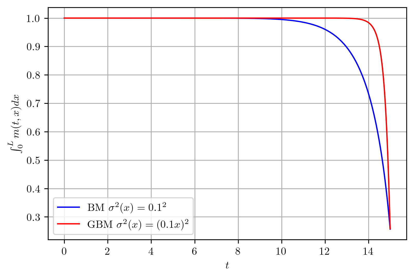
Figure 7: Total remaining mass in test 1 (BM) and (GBM)

5.2.2 Parameters sensitivity tests

We plot the time evolution of price and aggregate production as the parameters in the model change in a range of value. In these examples we fix $L=6$, $T=15$, $E=3$, unless otherwise specified, and use the same discretization as in the first test. $m_{0}$ is chosen as in Eq. 58.

Figure 8: Price (left) and production (right) with $T=15$, $\sigma=0.05$, $\eta=1.2$, $\rho=0$, $\delta=0.2$, $\kappa=5$ and different $\gamma$

Figure 9: Price (left) and production (right) with $T=15$, $\sigma=0.05$, $\eta=1.2$, $\rho=0$, $\delta=0.2$, $\gamma=4$ and different $\kappa$

Figure 10: Price (left) and production (right) with $T=15$, $\sigma=0.05$, $\eta=1.2$, $\rho=0$, $\gamma=4$, $\kappa=5$ and different $\delta$

Figure 11: Price (left) and production (right) with $T=15$, $\sigma=0.05$, $\eta=1.2$, $\delta=0.2$, $\gamma=4$, $\kappa=5$ and different $\rho$

Figure 12: Price (left) and production (right) with $T=30$, $\sigma=0.05$, $\eta=1.2$, $\delta=0.2$, $\gamma=4$, $\kappa=5$ and different $\rho$

Figure 13: Price (left) and production (right) with $T=15$, $\lambda=\rho=0$, $\eta=1.2$, $\delta=0.2$, $\gamma=4$, $\kappa=5$ and different $\sigma$

Figure 14: Total remaining mass with $T=15$, $\lambda=\rho=0$, $\eta=1.2$, $\delta=0.2$, $\gamma=4$, $\kappa=5$ and different $\sigma$

Figure 15: Price (left) and production (right) with $T=15$, $\rho=0$, $\eta=1.2$, $\delta=0.2$, $\gamma=4$, $\kappa=5$, $\sigma=0.1$

We make the following observations:

• Higher production cost (higher $\gamma$ or $\kappa$) leads to higher price and lower aggregate production, see Fig. 8 and Fig. 9.

• Lower price of subsitutes (higher $\delta$) leads to lower price and lower production, see Fig. 10.

• With negative $\rho$, agents feel more urge to produce. With larger $\rho$, agents may produce less at the beginning and save the reserve for producing later, see Fig. 11. In fact, if we consider a longer time horizon, it might be that producers hoard their reserve for a significant period of time, see Fig. 12. For $\rho>0$, the price would have increase exponentially in time if aggregate production remains constant. However, production tends to increase such that the price increases almost only linearly, as can be observed in Fig. 11. This is more clear in Fig. 12 with $\rho=0.09$, as price was increasing exponentially until production starts.

• If we use a small viscosity (e.g. $\sigma=0.05$), aggregate production and price remain almost constant until near the terminal time. We can see from Fig. 13 that aggregate production and price are, respectively, deceasing and increasing with respect to the diffusion coefficient. A plausible partial explanation is related to the left boundary condition. With large $\sigma$, one’s remaining resources are more likely to hit $0$ even if one is producing nothing. As in Fig. 14, higher $\sigma$ leads to faster decay of $\int_{0}^{L}m(t,x)dx$.

• $\lambda$ is the subjective discount which describes the producers’ time preference. We can see from Fig. 15 that with higher $\lambda$, the aggregate production tends to be higher at the early stage.

5.2.3 A model of oil production

In this example we consider the oil production model in [27, Section 3.2.2], see also [26] for more details. The price function is defined by Eq. 10 and the diffusion is GBM, i.e. $\sigma^{2}(x)=(\sigma x)^{2}$. The parameters are taken as, following [26, p. 36]:

$$L=60,\,\,T=150,\,\sigma=0.05,\,\lambda=0.05,\,\gamma=10,\,\kappa=50,\,E=40,\,\rho=0.02,\,\eta=1.2,\,\delta=0.1.$$ (59)

For space and time discretization, we use $N_{x}=600$ and $N_{t}=1500$ so that $\Delta t=h=0.1$.

Figure 16: Evolution of price (left) and aggregate production (right)

Figure 17: Evolution of density in the oil production model

We have obtained in Fig. 16 the same results as Guéant, Lasry and Lions [26, Fig. 8 and Fig 9, p. 36-37]. Fig. 17 shows the evolution of reserve density and total mass over time. As mentioned in  [26], oil production increases and then decreases, which can be viewed as a form of the so-called Hubbert peak.

Acknowledgment. The authors thank Jiahao Song for contributions to the numerical simulations section.