Algorithmic Decision-Making under Agents with Persistent Improvement
Abstract
This paper studies algorithmic decision-making under human’s strategic behavior, where a decision maker uses an algorithm to make decisions about human agents, and the latter with information about the algorithm may exert effort strategically and improve to receive favorable decisions. Unlike prior works that assume agents benefit from their efforts immediately, we consider realistic scenarios where the impacts of these efforts are persistent and agents benefit from efforts by making improvements gradually. We first develop a dynamic model to characterize persistent improvements and based on this construct a Stackelberg game to model the interplay between agents and the decision-maker. We analytically characterize the equilibrium strategies and identify conditions under which agents have incentives to improve. With the dynamics, we then study how the decision-maker can design an optimal policy to incentivize the largest improvements inside the agent population. We also extend the model to settings where 1) agents may be dishonest and game the algorithm into making favorable but erroneous decisions; 2) honest efforts are forgettable and not sufficient to guarantee persistent improvements. With the extended models, we further examine conditions under which agents prefer honest efforts over dishonest behavior and the impacts of forgettable efforts.
1 Introduction
In applications such as lending, college admission, hiring, etc., machine learning (ML) algorithms have been increasingly used to evaluate and make decisions about human agents. Given information about an algorithm, agents subject to ML decisions may behave strategically to receive favorable decisions. How to characterize the strategic interplay between algorithmic decisions and agents, and analyze the impacts they each have on the other, are of great importance but challenging.
This paper studies algorithmic decision-making under strategic agent behavior. Specifically, we consider a decision-maker who assesses a group of agents and aims to accept those that are qualified for certain tasks based on assessment outcomes. With knowledge of the acceptance rule, agents may behave strategically to increase their chances of getting accepted. For example, agents may invest to genuinely improve their qualifications (i.e., honest effort), or they may manipulate the observable assessment outcomes to game the algorithm (i.e., dishonest effort). Both types of behaviors have been studied. In particular, Hardt et al. (2016a); Dong et al. (2018); Braverman and Garg (2020); Jagadeesan et al. (2021); Sundaram et al. (2021); Zhang et al. (2022); Eilat et al. (2022) focus on learning under strategic manipulation, where they proposed various analytical frameworks (e.g., Stackelberg games) to model manipulative behavior, and analyzed models or developed learning algorithms that are robust against manipulation.
Another line of research (Zhang et al., 2020; Harris et al., 2021; Bechavod et al., 2022; Kleinberg and Raghavan, 2020; Chen et al., 2020; Barsotti et al., 2022; Jin et al., 2022) considers a different setting where agent qualifications (labels) change in accordance with the improvement actions. The goal of the decision-maker is to design a mechanism such that agents are incentivized to behave toward directions that improve the underlying qualifications. Notably, Kleinberg and Raghavan (2020) proposed a mechanism to incentivize individuals to invest in specific improvable features. Their work inherited the classical settings of the Principal-agent model in economics but designed an incentivizing mechanism under a linear classifier. They modeled manipulation and improvement similarly (linear in efforts) and did not consider the persistent and delayed effects of improvement. The mixture of both improvement and manipulation behavior is also studied (Miller et al., 2020; Chen et al., 2020; Barsotti et al., 2022; Horowitz and Rosenfeld, 2023). However, these works regarded improvement as a similar action to manipulation where the only difference is it will incur a label change. Another related topic is performative prediction (Perdomo et al., 2020; Izzo et al., 2021; Hardt et al., 2022; Jin et al., 2024), an abstraction that captures agent actions via model-induced distribution shifts. Details and more related works are presented in Appendix C.
This paper primarily focuses on honest agents with improvement, while settings with both improvement and manipulation are also studied. We first propose a novel two-stage Stackelberg game to model the interactions between decision-maker and agents, i.e., the decision-maker commits to its policy, following which agents best respond. A crucial difference between this study and the prior works is that the existing models all assume that the results of agents’ improvement actions are immediate, i.e., once agents decide to improve, they experience sudden changes in qualifications and receive the return at once. However, we observe that in many real-world applications, the impacts of improvement action are indeed persistent and delayed. For example, humans improve their abilities by acquiring new knowledge, but they make progress gradually and benefit from such behavior throughout their lifetime; loan applicants improve their credit behaviors by repaying all the debt in time, but there is a time lag between such behaviors and the increase in their credit scores. Therefore, it is critical to capture these delayed outcomes in the Stackelberg game formulation.
To this end, we propose a qualification dynamic model to characterize how agent qualifications would gradually improve upon exerting honest efforts. Such dynamics further indicate the time it takes for agents to reach the targeted qualifications that are just enough for them to be accepted. The impacts of such time lag on agents are then captured by a discounted utility model, i.e., reward an agent receives from the acceptance diminishes as time lag increases. Under this discounted utility model, agents best respond by determining how much effort to exert that maximizes their discounted utilities.
This paper aims to analytically and empirically study the proposed model. With the understanding of the strategic interactions between the decision-maker and agents, we further study how the decision-maker can design an optimal policy to incentivize the largest improvements inside the agent population, and empirically verify the benefits of the optimal policy.
Additionally, we extend the model to more complex settings where (i) agents have an additional option of strategic manipulation and can exert dishonest effort to game the algorithm; (ii) honest efforts exerted by agents are forgettable and may not be sufficient to guarantee persistent improvements, instead the qualifications may deteriorate back to the initial states. We will propose a model with both manipulation & improvement and a forgetting mechanism to study these settings, respectively. We aim to examine how agents would behave when they have both options of manipulation and improvement, under what conditions they prefer improvement over manipulation, and how the forgetting mechanism affects an agent’s behavior and long-term qualifications.
Our contributions can be summarized as follows:
-
1.
We formulate a new Stackelberg game to model the interactions between decision-maker and strategic agents. To the best of our knowledge, this is the first work capturing the delayed and persistent impacts of agents’ improvement behavior (Sec. 2).
-
2.
We study the impacts of acceptance policy and the external environment on agents, and identify conditions under which agents have incentives to exert honest efforts. This provides guidance on designing incentive mechanisms to encourage agents to improve (Sec. 3).
-
3.
We characterize the optimal policy for the decision-maker that incentivizes the agents to improve (Sec. 4).
-
4.
We consider the possibility of dishonest behavior and propose a model with both improvement and manipulation; we identify conditions when agents prefer one behavior over the other (Sec. 5).
-
5.
We propose a forgetting mechanism to examine what happens when honest efforts are not sufficient to guarantee persistent improvement (Sec. 6).
-
6.
We conduct experiments on real-world data to evaluate the analytical model and results (Sec. 7).
2 Problem Formulation
Consider an agent population with skill sets. Each agent has a qualification profile at time , denoted as a unit -dimensional vector with , A decision-maker at each time makes decisions (“0" being reject and “1" accept) about the agents based on their qualification profiles. Let fixed vector be the ideal qualification profile that the decision maker desires.
Decision-maker’s policy. For an agent with qualification profile , the decision-maker assesses whether the agent’s profile lines up with the desired qualifications , and makes decision based on their similarity using a fixed threshold policy , i.e., only agents that are sufficiently fit can get accepted. How to choose threshold is discussed in Sec. 4. We assume only agents with initial similarity are interested in positions and only focus on these candidates.
Although the decision policy introduced above focuses on the similarity between and where qualifications are normalized with the same magnitude for all agents, it can be easily extended to settings where the magnitude/strength of skills also matters and may differ across agents. Specifically, we propose a pre-normalization procedure to account for the strength of skills. The idea is to first add an additional dimension to initial qualification profile , which represents the agent’s unobservable “irrelevant attribute" (all other skills an agent has that are not important for the decision). Meanwhile, we add this dimension to ideal qualification profile with 0 as its value. We can make a natural assumption that after adding the dimension of “irrelevant attribute", the norm of -dimensional complete profile is the same for all agents. This is reasonable and supported by the literature (Liu et al., 2022; Holmstrom and Milgrom, 1991), which suggests that when qualification profiles are multi-dimensional, the competency in relevant/measurable attributes implies the weakness in irrelevant/unmeasurable attributes. The detailed pre-normalization procedure is formally presented in Algorithm 1 (App. A).
Agent qualification dynamics. We assume agents have information about the ideal profile (e.g., from application guides, mock interviews). In the beginning, agents with can choose to improve their profiles by investing an effort to acquire the relevant knowledge, but the effort will have delayed and persistent effects over subsequent time stages. The specific value of depends on the agent’s utility and will be introduced at the end of this section. Upon investing , the agent’s qualifications gradually improve over time based on the following:
| (1) |
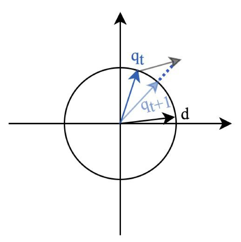
(1) suggests that agents at each time improve toward the ideal profile . How much they can improve depend on their current profile and the effort . The similarity in the dynamics captures the reinforcing effects: agents that are more qualified could have more resources and are more capable of leveraging the acquired knowledge to improve their skills. Note that the maximum improvement an agent attains at each round is bounded, i.e., the normalized vector after improvement is always between current qualifications and the ideal profile . Fig. 1 illustrates the improvement dynamics of qualification in a two-dimensional space.
Dynamics in (1) model the delayed and persistent impacts of improvement action (i.e., effort ). In many real applications, humans acquire knowledge and benefit from repeated practices. They make progress toward the goal gradually, and it takes time to receive the desired outcome from the investment. Indeed, (1) is inspired by the dynamics in Dean and Morgenstern (2022), which was used for modeling preference shifts (details are in App. C.3), where individuals update their opinions/preferences based on their correlations with some influencer (e.g., a political figure) and control the power of the intervention. We believe this is similar to improvement especially when agents improve themselves by imitating some "role models". For example, in a job application scenario, the “influencer” is a current worker who holds information session and introduces her profile . Then the agents strive to mimic the profile of by updating . The imitating nature of improvement is well justified in many works (e.g., Raab and Liu (2021); Zhang et al. (2022)), making agent improvement suitable to be modeled in a similar fashion to concept drift/preference shift. Thus, we use (1) to model the evolution of agents’ (pre-normalized) qualifications. Based on Prop. 1 of Dean and Morgenstern (2022), we know that converges under dynamics, as formally stated in Lemma 2.1 below.
Lemma 2.1 (Convergence of qualification).
Consider an agent with initial similarity . If he/she makes an effort and improves qualification profile based on dynamics in (1), then converges to the desired profile . The evolution of the similarity is given by:
| (2) |
Lemma 2.1 suggests that any agent eventually becomes an ideal candidate with a perfectly aligned profile (i.e., ), as long as he/she is interested in the position () and willing to make an effort (). The only difference among agents is the speed of convergence: it takes less time for agents who are more qualified at the beginning (i.e., larger ) and/or make more effort (i.e., larger ) to become ideal and get accepted. Note that our work focuses on agent’s improvement behavior with persistent and delayed effects. Although the model is presented in a simplified setting where only a one-step effort is made by the agents at the beginning, it can capture more complicated scenarios where agents repeatedly exert efforts multiple times until they reach the target. Each effort has persistent effects on improving the qualification. Specifically, suppose each agent at time can exert an effort and the agent’s qualification improves based on with (i.e., every time the agent improves from all accumulated efforts he/she invested so far). For this new dynamics, the overall impacts of these efforts on improving agent qualification can be equivalently characterized by the dynamics (1) with some one-step effort. That is, there exists an effort such that investing once at the beginning has the same impact on as investing a sequence of efforts over time. We provide more detailed discussion on this in App. B. We also discuss a special case where the effect of is decreasing over time and provide further convergence analysis in App. B.
Agent’s utility & action. Because it takes time for agents to receive rewards (i.e., get accepted) for their efforts, they may not have incentives to invest if there is a long delay. In practice, people may be more attracted to investments with immediate rewards than delayed rewards, or they may simply not have enough time to wait. For example, students only have limited time to prepare for college applications; credit card applicants may not have incentives to improve their credit scores and wait to get approval for a specific credit card when there are many instant-approval cards on the market.
To characterize the delayed rewards, we use a discount model and assume the reward each agent receives from the effort decreases over time. Specifically, let be the minimum time it takes for an agent to get accepted from the effort . We define agent’s utility as:
| (3) |
That is, the utility is the exponentially discounted reward an agent receives from the acceptance minus the effort. is the discounting factor. Note that the discounted utility model111Under exponential discounting function, the agent’s reward diminishes at a constant rate (Grüne-Yanoff, 2015). Our model can also adopt other discounting functions (e.g., hyperbolic discounting) for settings when the agent’s reward decreases inconsistently. The qualitative results of this paper still remain the same. has been widely used in literature such as reinforcement learning (Kaelbling et al., 1996), finance (Meier and Sprenger, 2013), and economics (Krahn and Gafni, 1993; Samuelson, 1937).
Since threshold policy is used to make decisions, an agent gets accepted whenever the qualification profile is sufficiently aligned with the ideal profile, i.e., . Based on (2), we can derive as a function of threshold , agent’s initial similarity , and effort , i.e.,
| (4) | |||||
Plug in (3), agent’s utility becomes:
| (5) |
Therefore, strategic agents will choose to improve their qualifications only if utility , and they will choose the investment that maximizes the utility.
Stackelberg game. We model the strategic interplay between the decision-maker and agents as a Stackelberg game, which consists of two stages: (i) the decision-maker first publishes the optimal acceptance threshold (details are in Sec. 4); (ii) agents after observing the threshold take actions to maximize their utilities as given in (5).
Manipulation & forgetting. The model formulated above has two implicit assumptions: (i) agents are honest and they improve their qualifications by making actual efforts; (ii) once agents make a one-time effort to acquire the knowledge, they never forget and can repeatedly leverage this knowledge to improve their profiles based on (1). However, these assumptions may not hold. In practice, agents may fool the decision-maker by directly manipulating to get accepted without improving actual , e.g., people cheat on exams or interviews to get accepted. Moreover, the knowledge agents acquired at the beginning may not be sufficient to ensure repeated improvements.
To capture these, we further extend the above model to two settings:
-
1.
Manipulation: Besides improving the actual profile by making an effort , agents may choose to manipulate directly to fool the decision-maker. The detailed model and analysis are in Sec. 5.
-
2.
Forgetting: One-time investment may not guarantee the improvements all the time, i.e., qualifications do not always move toward the direction of ideal profile , instead it may devolve and possibly go back to starting state . The detailed model and analysis are in Sec. 6.
Objective. In this paper, we study the above interactions between decision-maker and agents. We aim to understand (i) under what conditions agents have incentives to improve their qualifications; (ii) how to design the optimal policy to incentivize the largest improvements inside the agent population; (iii) how the agents would behave when they have both options of manipulation and improvement, and under what conditions agents prefer improvement over manipulation; (iv) how the forgetting mechanism affects agent’s behavior and long-term qualifications.
3 Improvement & Optimal Effort
In this section, we examine the impact of decision threshold and the environment (i.e., discounting factor ) on agent behavior. Specifically, we focus on agents with discounted utility ((5)) and identify conditions under which the agents have incentives to improve their qualifications. Note that we do not consider issues of manipulation and forgetting in this section. Based on (5), an agent with chooses to improve only if its utility . To characterize the impact of an agent’s one-time investment on , we first define a function that summarizes the impacts of all the other factors (i.e., threshold , discounting factor , and initial profile similarity ) on agent utility, as defined below.
| (6) |
Based on , we can derive conditions under which agents have incentives to improve (Thm. 3.1).
Theorem 3.1 (Improvement & optimal effort).
There exists a threshold such that for any that satisfies , the agent has the incentive to improve the qualifications, i.e., agent utility is positive for some efforts . Moreover, there exists a unique optimal effort that maximizes the agent utility.
Thm. 3.1 identifies a condition under which agents have incentives to exert positive effort . This condition depends on factors and can be fully characterized by the function .
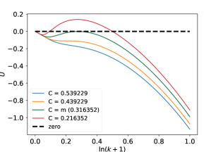
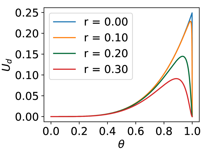
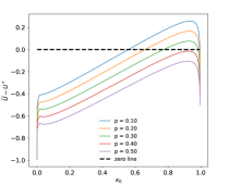
Although the analytical solution of the threshold is difficult to find, we can numerically solve as shown in App. H.1. In Fig. 2, we illustrate agent utilities as functions of effort under different . The results show that only when (red curve), an agent can attain positive utility with effort ; when (green/yellow/blue curve), agents will not invest because the maximum utility is attained at . Moreover, when (red curve), there is a unique optimal effort that maximizes the utility. These results are consistent with Thm. 3.1.
The condition in Thm. 3.1 further indicates the impacts of policy , discounting factor , and initial state on agent behavior. Specifically, agents only invest if holds. By fixing any two of , we can identify the domain of the third factor under which agents invest to improve. These results are summarized in Table 1 and verified in App. D. It shows that for any threshold and discounting factor , agents only improve if their initial qualification profile is sufficiently similar to the ideal profile; the domain of also implies the best profile an agent with initial state can reach after exerting effort: if acceptance threshold is larger than the upper bound of given in Table 1, then agents will not have incentives to improve.
| Domain of (given ) | |
|---|---|
| Domain of (given ) |
The above results further suggest effective strategies that encourage agents to improve their qualifications, i.e., more agents are incentivized to improve if (i) the decision-maker’s acceptance threshold is lower; or (ii) the time it takes for agents to succeed after investments is shorter (smaller discounting factor ). Examples of both strategies in real applications are discussed in App. D, which further verify the effectiveness of our proposed model.
4 Decision-maker’s policy to incentivize improvement
Sec. 3 studied the impact of threshold on agent behavior and provided guidance on incentivizing agents to improve. In practice, although it is more difficult to adjust the discounting factor , the decision-maker can adjust the threshold policy to incentivize the largest possible amount of total improvement, thereby improving the social welfare. In this section, we study the optimal policy when the decision-maker is aware of the agent’s best response and hopes to incentivize agents to improve.
Suppose the decision-maker has full information about agents and can anticipate their behaviors, i.e., for any decision threshold , it knows that agents whose initial similarity will invest and improve their profiles (by Table 1). Also, we define to let be continuous in and denote as the probability density function of the agent similarity which is also continuous in . Then, we can define as the utility of the decision-maker under the threshold as the total amount of agents’ improvements:
| (7) |
Eq. (7) above demonstrates that the decision-maker aims to maximize the total improvement among the agent population, and its utility is a function of . Since are both continuous in , utility is also continuous. The following Thm. 4.1 further shows the existence of the optimal thresholds .
Theorem 4.1 (Existence of optimal threshold).
For any decision-maker with utility function , there exists at least one that is optimal under which . Moreover, is the unique optimal point of if has one root within .
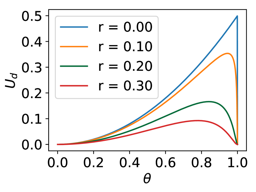
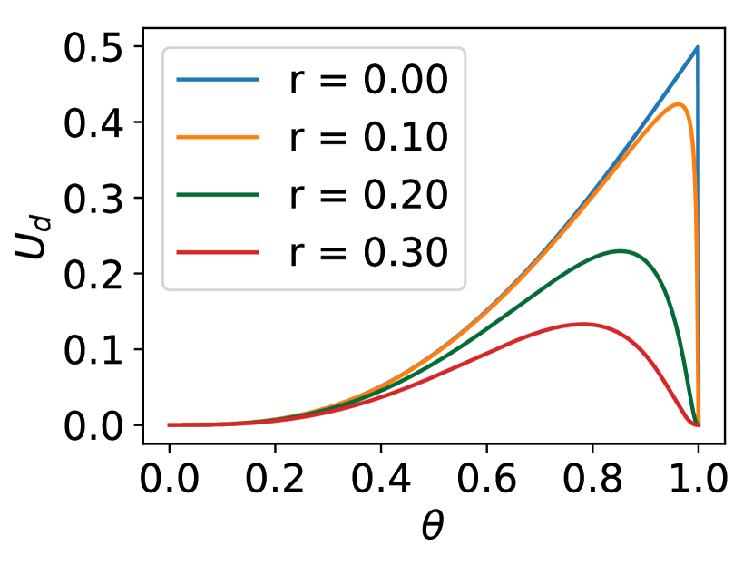
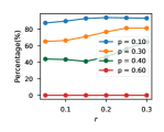
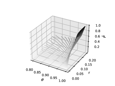
To verify Thm. 4.1, we demonstrate the values of under situations where the agent population has different density functions and different discounting factors . Specifically, we consider the uniform distribution and Beta distributions with different parameters. Fig. 3 shows under different density functions and discounting factors . The results illustrate that under these settings, is single-peaked and there is a unique that is optimal and results in positive utility, which is consistent with Thm. 4.1. The figure also indicates the impact of on the optimal threshold: as increases, increases and the corresponding maximum utility decreases. As formally stated below in Corollary 4.2. We prove Thm. 4.1 and Corollary 4.2 in App. H.2.
Corollary 4.2.
For that has a unique maximizer , optimal decreases as increases.
Importantly, the results of Thm. 4.1 show that the decision-maker can always find an optimal decision threshold (either numerically or using gradient methods depending on the density function ) to incentivize the largest improvement and promote social welfare in practice. While the above results all assume the decision-maker knows when determining , we can relax this and provide a procedure to estimate ; this is included in App. G.
5 Impact of Manipulative Behavior
Our analysis and results so far rely on an implicit assumption that agents are honest and they improve qualifications by making actual efforts. However, as mentioned in Sec. 2, agents in practice may fool the decision-maker by strategically manipulating to get accepted without improving . Next, we extend our model in Sec. 2 by considering the possibility of such manipulative behavior.
Model with both manipulation & improvement. We extend the model in Sec. 2 where agents after observing have an additional option to manipulate directly. If they choose to improve, they make a one-time effort to acquire relevant knowledge and gradually improve their qualifications over time based on (1). If they choose to manipulate, they only increase at every round to fool the decision-maker without changing the actual profile . Similar to the literature on strategic classification (Hardt et al., 2016a), the manipulation comes at the cost and the risk of being caught.
Specifically, let be the manipulation cost it takes for an agent to increase its similarity from to , and be the detection probability of manipulation during an agent’s entire application process. Agents, once getting caught manipulating , will never be accepted.
Degree of manipulation. If agents choose to manipulate, they will increase at every round to fool the decision-maker, and they manipulate in a way that minimizes the manipulation cost and the risk of being detected. We make the following natural assumptions on and :
-
1.
Let be the best outcome agents can attain from at round by improvement behavior (with largest effort ). If for some , then because the decision-maker can be certain that is the result of manipulation; otherwise, if .
-
2.
The total manipulation cost it takes for an agent with initial similarity to be accepted is .
Note that above indicates the maximum degree of manipulation of agents: to avoid being detected, an agent should not manipulate more than . We can compute directly from Lemma 2.1 (by setting ), i.e., . For agents who manipulate, if the total manipulation cost needed to get accepted is and detection probability whenever , then agents will always manipulate toward to maximize its utility. As a result, agents who manipulate can be regarded as they mimic the improvement behavior with the largest effort .
Let be agent’s utility under manipulation, which is the benefit an agent obtains from acceptance (when not being detected) minus the manipulation cost, i.e.,
| (8) |
where the benefit is derived based on (5) (with ).
Agent’s best response. Suppose agents have full information about detection probability and discounting factor , after observing the acceptance threshold , they best respond by choosing the action (i.e., improvement/manipulation/do nothing) that maximizes their utilities, i.e., if , they choose to manipulate; otherwise, they improve by exerting optimal effort .
Next, we examine under what conditions agents prefer improvement over manipulation.
Theorem 5.1.
Suppose manipulation cost and threshold for some . For any discounting factor , there exists such that the followings hold:
1. If , then such that agents manipulate only when initial similarity .
2. If , then such that agents manipulate only when initial .
3. If , then agents never choose to manipulate.
Thm. 5.1 considers scenarios when the threshold is sufficiently high, and identifies conditions under which manipulation is preferred by agents in these settings. It shows agent behavior highly depends on the risk of manipulation (i.e., detection probability ). The specific values of , , , in Thm. 5.1 depend on , . In particular, increases as increases. Indeed, we can empirically find , , , and verify the theorem. These are illustrated in App. E and Sec. 7.
6 Forgetting Mechanism
The analysis in previous sections relies on the assumption that once agents make a one-time effort to acquire the knowledge, they never forget and can repeatedly leverage this knowledge to improve their profiles based on (1). This may not hold in practice when the knowledge agents acquired at the beginning are not sufficient to guarantee repeated improvements. In this section, we extend the qualification dynamics ((1)) by incorporating the forgetting mechanism, i.e., qualification profile does not always move toward the direction of ideal profile , instead, it may devolve and possibly go back to the initial . Note that we only consider honest agents who do not manipulate. By modifying (1), we define the new qualification dynamics with forgetting as follows.
| (9) | |||||
Let , then new dynamics in (9) implies that at each round, qualification profile is pushed toward the direction of , i.e., a convex combination of ideal profile and initial qualifications . Whether improves towards or deteriorates back to depends on the investment : with more effort , the degree of forgetting is less; there is no forgetting if all the knowledge is acquired (). Under the new dynamics, we can derive the convergence of the qualification profile as follows.
Theorem 6.1 (Convergence of qualification under forgetting).
Consider an agent with initial similarity whose qualifications follow dynamics in (9). Suppose the agent makes investment , then converges to profile and the similarity satisfies:
| (10) |
where , , and .
Thm. 6.1 implies that convergence still holds when qualifications evolve with forgetting. Unlike the scenarios without forgetting where eventually converges to the ideal profile regardless of (Lemma 2.1), now converges to , i.e., a profile between initial qualifications and ideal profile , which is closer to with smaller investment . It shows that if agents do not exert enough effort and the acquired knowledge is not sufficient, then they will not make satisfactory improvements.
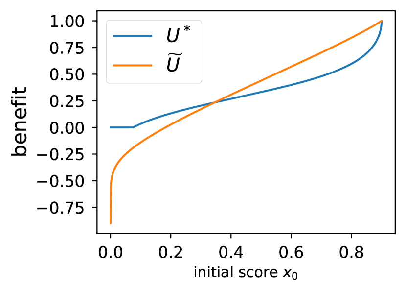
Agent’s utility and improvement action. Denote agent utility under the forgetting mechanism as . Unlike settings without forgetting where we can derive the exact time it takes for agents to be accepted and find utility ((5)), the analytical form of is not easy to derive. Nonetheless, we can still show that there exist scenarios under which agents have incentives to improve, even though the best attainable profile is a profile between initial and the ideal .
Theorem 6.2.
For any threshold (resp. discounting factor ), there exists a discounting factor (resp. threshold ) such that agent’s utility for some , i.e., agents have the incentive to make a positive effort. The upper bound of the optimal effort is given by
where is the root of within .
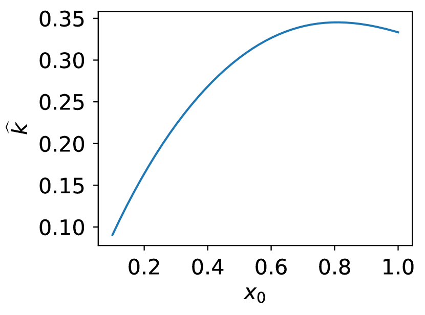
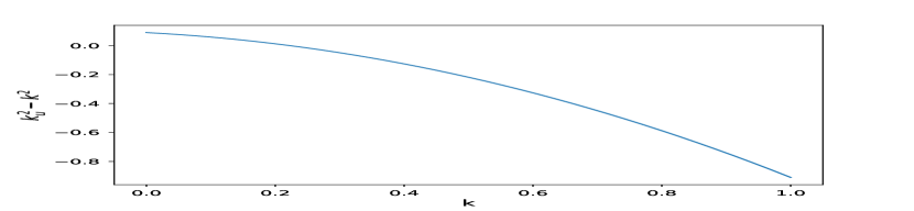
Thm. 6.2 implies that there exists such that agents best respond by improving their qualifications, and the optimal effort is upper bounded by . Indeed, we can numerically find the upper bound as a function (shown in Fig. 4). Because for all , the improvement an agent can make under the forgetting mechanism is limited, suggesting that the agents may not improve to be qualified when the tasks are challenging enough.
Remark.
Under the forgetting mechanism, the actual effort invested by any agent is less than 0.35, and the qualifications converge to a profile that is between and .
7 Experiments

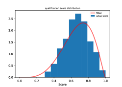
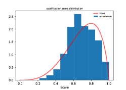
We validate theoretical results by conducting experiments on Exam score (Kimmons, 2012) and FICO score (Reserve, 2007) dataset. For both datasets, scores serve as the agent’s initial similarity , and we assume agents interact with a decision maker based on the Stackelberg game in Sec. 2. We first fit these scores with beta distributions, i.e., , and then use them to derive the followings:
-
1.
The optimal decision threshold for the decision-maker to incentivize the largest amount of improvement and promote social welfare, and the total improvement induced by .
-
2.
The percentage of agents who choose to manipulate under the decision-maker’s optimal policy.
Exam Score Data. It is a synthetic dataset containing 1000 students’ exam scores on 3 subjects including math, reading, and writing (Kimmons, 2012). We first average over 3 subjects and normalize the averaged score to . Then, we fit two beta distributions to the normalized scores of males and females and obtain (see Fig. 9 in App. F).
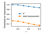
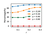
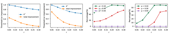
With these distributions, we can compute the optimal decision thresholds and the corresponding total improvement under different discounting factors . As shown in Fig. 5, for both males and females, the experimental results are similar. When increases, always decreases and the total amount of improvement becomes lower. This illustrates how larger discounting factors harm agents’ improvement. Additionally, we consider settings with both manipulation and improvement. Fig. 5 also shows the percentages of agents who prefer to manipulate under . It shows that agents are less likely to manipulate as detection probability increases.
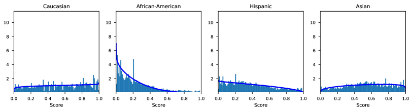
FICO Score Data. We adopt the data pre-processed by Hardt et al. (2016b), which contains CDF of credit scores of four racial groups (Caucasian, African American, Hispanic, Asian). For each group, we fit a Beta distribution and obtain four distributions: for Caucasian, for African American, for Hispanic, for Asian (see Fig. 10 in App. F). We only present the results for Caucasians and African Americans, while the results for Asian and Hispanic are shown in App. F.
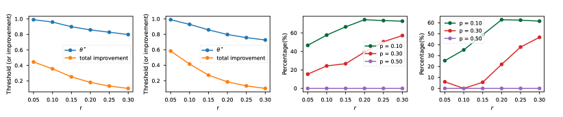
For each group, we compute the optimal decision threshold and corresponding total improvement under different . As shown in Fig. 6 (left two plots), for both groups, their corresponding optimal threshold and the total amount of improvement always decrease as increases. For settings with both manipulation and improvement (right two plots in Fig. 6), agents are more likely to manipulate under smaller detection probability. When detection probability is sufficiently large, agents do not have incentives to manipulate.
8 Conclusions & Limitations
This paper studies the strategic interactions between agents and a decision-maker when agent action has delayed and persistent effects. By utilizing a qualification dynamics model and the discounting utility function, we analyze the conditions where agents tend to improve and investigate how the decision-maker can incentivize agents to make the largest improvement. Moreover, we consider the situation where agents can improve or manipulate, and characterize how agents would make improvement or manipulation decisions when their efforts take time to pay back. Finally, we discuss the situation where the tasks are challenging and a forgetting mechanism takes place, thereby expanding the scope of our model.
However, our theoretical results depend on the assumption that both agents and the decision-maker have perfect information about each other so that they always best respond. Extension to cases when each party only has partial or imperfect information is important. Moreover, these theorems are based on the qualification dynamics (1). Although a scenario when it does not hold is studied in Sec. 6, future works should also consider other variants tailored to specific applications to prevent negative outcomes.
Impact Statement
We believe our work fills the gap in which agent strategic behaviors are benign and agents’ efforts can have long-lasting but diminishing effects. This can be the case under many real-world situations including exam preparation and job application. Thus, our model can improve trustworthy machine learning and decision-making in reality. However, as mentioned in Sec. 8, our work relies on certain assumptions and needs to be used cautiously. Moreover, though we provide a procedure to estimate the discounting factor, performing controlled experiments is not always accessible. Meanwhile, manipulation cost and detection probability are unknown and hard to estimate. Collecting real data and estimating these parameters remain promising research directions in the future.
References
- Ahmadi et al. (2021) Saba Ahmadi, Hedyeh Beyhaghi, Avrim Blum, and Keziah Naggita. The strategic perceptron. In Proceedings of the 22nd ACM Conference on Economics and Computation, pages 6–25, 2021.
- Ahmadi et al. (2022a) Saba Ahmadi, Hedyeh Beyhaghi, Avrim Blum, and Keziah Naggita. On classification of strategic agents who can both game and improve. arXiv preprint arXiv:2203.00124, 2022a.
- Ahmadi et al. (2022b) Saba Ahmadi, Hedyeh Beyhaghi, Avrim Blum, and Keziah Naggita. Setting fair incentives to maximize improvement. arXiv preprint arXiv:2203.00134, 2022b.
- Alon et al. (2020) Tal Alon, Magdalen Dobson, Ariel Procaccia, Inbal Talgam-Cohen, and Jamie Tucker-Foltz. Multiagent evaluation mechanisms. Proceedings of the AAAI Conference on Artificial Intelligence, 34:1774–1781, 2020.
- Barsotti et al. (2022) Flavia Barsotti, Ruya Gokhan Kocer, and Fernando P. Santos. Transparency, detection and imitation in strategic classification. In Proceedings of the Thirty-First International Joint Conference on Artificial Intelligence, IJCAI-22, pages 67–73, 2022.
- Bechavod et al. (2021) Yahav Bechavod, Katrina Ligett, Steven Wu, and Juba Ziani. Gaming helps! learning from strategic interactions in natural dynamics. In International Conference on Artificial Intelligence and Statistics, pages 1234–1242, 2021.
- Bechavod et al. (2022) Yahav Bechavod, Chara Podimata, Steven Wu, and Juba Ziani. Information discrepancy in strategic learning. In International Conference on Machine Learning, pages 1691–1715, 2022.
- Ben-Porat and Tennenholtz (2017) Omer Ben-Porat and Moshe Tennenholtz. Best response regression. In Advances in Neural Information Processing Systems, 2017.
- Braverman and Garg (2020) Mark Braverman and Sumegha Garg. The role of randomness and noise in strategic classification. CoRR, abs/2005.08377, 2020.
- Castellano et al. (2009) Claudio Castellano, Santo Fortunato, and Vittorio Loreto. Statistical physics of social dynamics. Reviews of modern physics, 81(2):591, 2009.
- Chen et al. (2020) Yatong Chen, Jialu Wang, and Yang Liu. Strategic recourse in linear classification. CoRR, abs/2011.00355, 2020.
- Dean and Morgenstern (2022) Sarah Dean and Jamie Morgenstern. Preference dynamics under personalized recommendations. In Proceedings of the 23rd ACM Conference on Economics and Computation, page 795–816, 2022.
- Dong et al. (2018) Jinshuo Dong, Aaron Roth, Zachary Schutzman, Bo Waggoner, and Zhiwei Steven Wu. Strategic classification from revealed preferences. In Proceedings of the 2018 ACM Conference on Economics and Computation, page 55–70, 2018.
- Eilat et al. (2022) Itay Eilat, Ben Finkelshtein, Chaim Baskin, and Nir Rosenfeld. Strategic classification with graph neural networks, 2022.
- Gaitonde et al. (2021) Jason Gaitonde, Jon Kleinberg, and Éva Tardos. Polarization in geometric opinion dynamics. In Proceedings of the 22nd ACM Conference on Economics and Computation, pages 499–519, 2021.
- Grüne-Yanoff (2015) Till Grüne-Yanoff. Models of temporal discounting 1937–2000: An interdisciplinary exchange between economics and psychology. Science in context, 28(4):675–713, 2015.
- Hardt et al. (2016a) Moritz Hardt, Nimrod Megiddo, Christos Papadimitriou, and Mary Wootters. Strategic classification. In Proceedings of the 2016 ACM Conference on Innovations in Theoretical Computer Science, page 111–122, 2016a.
- Hardt et al. (2016b) Moritz Hardt, Eric Price, Eric Price, and Nati Srebro. Equality of opportunity in supervised learning. In Advances in Neural Information Processing Systems, 2016b.
- Hardt et al. (2022) Moritz Hardt, Meena Jagadeesan, and Celestine Mendler-Dünner. Performative power. In Advances in Neural Information Processing Systems, 2022.
- Harris et al. (2021) Keegan Harris, Hoda Heidari, and Steven Z Wu. Stateful strategic regression. Advances in Neural Information Processing Systems, pages 28728–28741, 2021.
- Holmstrom and Milgrom (1991) Bengt Holmstrom and Paul Milgrom. Multitask principal–agent analyses: Incentive contracts, asset ownership, and job design. The Journal of Law, Economics, and Organization, pages 24–52, 1991.
- Horowitz and Rosenfeld (2023) Guy Horowitz and Nir Rosenfeld. Causal strategic classification: A tale of two shifts, 2023.
- Izzo et al. (2021) Zachary Izzo, Lexing Ying, and James Zou. How to learn when data reacts to your model: Performative gradient descent. In Proceedings of the 38th International Conference on Machine Learning, pages 4641–4650, 2021.
- Jagadeesan et al. (2021) Meena Jagadeesan, Celestine Mendler-Dünner, and Moritz Hardt. Alternative microfoundations for strategic classification. In Proceedings of the 38th International Conference on Machine Learning, pages 4687–4697, 2021.
- Jin et al. (2022) Kun Jin, Xueru Zhang, Mohammad Mahdi Khalili, Parinaz Naghizadeh, and Mingyan Liu. Incentive mechanisms for strategic classification and regression problems. In Proceedings of the 23rd ACM Conference on Economics and Computation, page 760–790, 2022.
- Jin et al. (2024) Kun Jin, Tongxin Yin, Zhongzhu Chen, Zeyu Sun, Xueru Zhang, Yang Liu, and Mingyan Liu. Performative federated learning: A solution to model-dependent and heterogeneous distribution shifts. In Proceedings of the AAAI Conference on Artificial Intelligence, volume 38, pages 12938–12946, 2024.
- Kaelbling et al. (1996) Leslie Pack Kaelbling, Michael L Littman, and Andrew W Moore. Reinforcement learning: A survey. Journal of artificial intelligence research, 4:237–285, 1996.
- Kimmons (2012) Royce Kimmons. Synthetic exam scores in a public school. Technical report, Brigham Young University, 2012.
- Kleinberg and Raghavan (2020) Jon Kleinberg and Manish Raghavan. How do classifiers induce agents to invest effort strategically? page 1–23, 2020.
- Krahn and Gafni (1993) Murray Krahn and Amiram Gafni. Discounting in the economic evaluation of health care interventions. Medical care, pages 403–418, 1993.
- Liu et al. (2019) Lydia T. Liu, Sarah Dean, Esther Rolf, Max Simchowitz, and Moritz Hardt. Delayed impact of fair machine learning. In Proceedings of the Twenty-Eighth International Joint Conference on Artificial Intelligence, IJCAI-19, pages 6196–6200, 2019.
- Liu et al. (2022) Lydia T. Liu, Nikhil Garg, and Christian Borgs. Strategic ranking. In Proceedings of The 25th International Conference on Artificial Intelligence and Statistics, pages 2489–2518, 2022.
- Meier and Sprenger (2013) Stephan Meier and Charles D Sprenger. Discounting financial literacy: Time preferences and participation in financial education programs. Journal of Economic Behavior & Organization, 95:159–174, 2013.
- Miller et al. (2020) John Miller, Smitha Milli, and Moritz Hardt. Strategic classification is causal modeling in disguise. In Proceedings of the 37th International Conference on Machine Learning, 2020.
- Perdomo et al. (2020) Juan Perdomo, Tijana Zrnic, Celestine Mendler-Dünner, and Moritz Hardt. Performative prediction. In Proceedings of the 37th International Conference on Machine Learning, pages 7599–7609, 2020.
- Raab and Liu (2021) Reilly Raab and Yang Liu. Unintended selection: Persistent qualification rate disparities and interventions. Advances in Neural Information Processing Systems, pages 26053–26065, 2021.
- Reserve (2007) United Federate Reserve. Report to the congress on credit scoring and its effects on the availability and affordability of credit. In Board of Governors of the Federal Reserve System, 2007.
- Rosenfeld et al. (2020) Nir Rosenfeld, Anna Hilgard, Sai Srivatsa Ravindranath, and David C Parkes. From predictions to decisions: Using lookahead regularization. In Advances in Neural Information Processing Systems, pages 4115–4126, 2020.
- Samuelson (1937) Paul A Samuelson. A note on measurement of utility. The review of economic studies, 4(2):155–161, 1937.
- Shavit et al. (2020) Yonadav Shavit, Benjamin L. Edelman, and Brian Axelrod. Causal strategic linear regression. In Proceedings of the 37th International Conference on Machine Learning, ICML’20, 2020.
- Sundaram et al. (2021) Ravi Sundaram, Anil Vullikanti, Haifeng Xu, and Fan Yao. Pac-learning for strategic classification. In Proceedings of the 38th International Conference on Machine Learning, pages 9978–9988, 2021.
- Zhang et al. (2020) Xueru Zhang, Ruibo Tu, Yang Liu, Mingyan Liu, Hedvig Kjellstrom, Kun Zhang, and Cheng Zhang. How do fair decisions fare in long-term qualification? In Advances in Neural Information Processing Systems, pages 18457–18469, 2020.
- Zhang et al. (2022) Xueru Zhang, Mohammad Mahdi Khalili, Kun Jin, Parinaz Naghizadeh, and Mingyan Liu. Fairness interventions as (Dis)Incentives for strategic manipulation. In Proceedings of the 39th International Conference on Machine Learning, pages 26239–26264, 2022.
Appendix A Pre-normalization
Though we focus on the similarity between and , magnitudes of do matter in many practical situations. For example, if the decision-maker prefers students with balanced math and English skills and there are two “balanced" students, the decision-maker will certainly prefer the one with higher scores. Therefore, we propose a pre-normalization procedure to incorporate magnitude into account. Specifically, we add an additional dimension representing the unobservable “irrelevant attributes” to and obtain a dimensional complete qualification profile. Meanwhile, we add an additional dimension to the ideal qualification profile with 0 as its value; the new ideal profile becomes . Then we can make the following natural assumption:
Assumption A.1.
After adding the dimension of “irrelevant attribute”, for all agents, the norms of their complete qualification profiles are the same.
Assumption A.1 has been supported by literature in machine learning Liu et al. (2022) and social science Holmstrom and Milgrom (1991). The “irrelevant" dimension demonstrates all other skills that belong to an agent but are not important to the decision. Therefore, competency in relevant/measurable attributes implies weakness in irrelevant/immeasurable attributes and the length of the complete qualification profile stays the same for all agents. With Assumption A.1 and the distribution of as , we formalize the pre-normalization procedure in Algorithm 1.
Appendix B Discussion and Generalization of (1)
More details on the dynamics in (1). In the main paper, we assume the influence of the initial effort is persistent and will enable changes gradually during each round. This is well-supported by the following examples:
-
1.
Creditworthiness: To improve creditworthiness, an individual may learn that an ideal profile would be a person with a constant high income and long-lasting good credit history. Therefore, she may exert a significant effort to find a job with a high salary. However, the effort will take several months or even one year for her to finally build up the ideal profile because she needs to work for a while to receive money and build a competitive credit history.
-
2.
Job application: An individual who wants to apply for a technology company may learn about the skill set of an ideal candidate from several resources (e.g., the job description, alumni who work at the company, info session) and then exert a significant effort to study the required knowledge. However, it still takes time for her to do exercises and master the skills, resulting in a delay of finally being qualified.
Model generalization when agents can invest efforts at different time steps. We discuss how the model in the main paper can capture more complicated scenarios where agents repeatedly exert efforts multiple times until they reach the target. Each effort has persistent effects on improving the qualification as shown in Eqn. (11).
| (11) | |||
where . This means the agents are able to invest more effort at arbitrary time steps (e.g., studying more skills in the middle of the preparing process), but the cumulative effort should not exceed 1 (they cannot master 110% of knowledge).
We first prove that there exists an effort such that investing once at the beginning has the same impact on as investing a sequence of efforts over time: define as the "what-if" qualifications if the agents invest or at the initial round. Since , we know the must be between . Then because is continuous with respect to , so we know must exist. Therefore, our model in the main paper can indeed assimilate the more complex setting.
Model generalization when diminishes with . In the main paper, is always equal to , demonstrating the effort has a consistent and persistent effect on the improvement of an individual. According to Lemma 2.1, the similarity approaches at an exponential rate. Thus, the case of is not interesting since the convergence is faster and it may not make sense in practice that the effort can be increasingly effective as time goes on. However, in reality, it may be possible that is decreasing. This is a “middle-point" case between the regular improvement in (1) and the forgetting mechanism (9), which may illustrate the “tiredness" when agents stick to improve. However, we can prove that when decreases linearly (i.e., ), the similarity can only converge to at a speed .
Theorem B.1.
When decreases linearly (i.e., ), converges to at a rate
We prove Thm. B.1 in App. H.5. Basically, this result illustrates that the agents will still improve to be qualified if decreases at a linear rate. Specifically, we can rewrite the (2) as:
| (12) |
From (12), we can derive similar results of the agents’ best responses and work out the thresholds for them to improve.
Appendix C Related Work
C.1 Strategic Manipulation
Though our work primarily lies in proposing a new model for improvement behaviors, the problem settings are also closely related to strategic classification problems Hardt et al. (2016a); Ben-Porat and Tennenholtz (2017); Dong et al. (2018); Braverman and Garg (2020); Sundaram et al. (2021); Jagadeesan et al. (2021); Ahmadi et al. (2021); Eilat et al. (2022); Horowitz and Rosenfeld (2023). Hardt et al. (2016a) formulated classification problems with strategic manipulation as a Stackelberg game with deterministic cost functions, where the decision maker optimizes classification accuracy based on individuals’ best responses. Afterwards, more sophisticated analytical frameworks were proposed Dong et al. (2018); Braverman and Garg (2020); Jagadeesan et al. (2021). Dong et al. (2018) proposed an online algorithm for strategic classification, and Braverman and Garg (2020) added randomness to strategic classifiers. On the other hand, Sundaram et al. (2021) analyzes the statistical learnability of strategic classification with an SVC classifier. Jagadeesan et al. (2021) relaxed the standard microfoundations assumption where individuals are perfectly rational to alternative microfoundations where a proportion of individuals may not be strategic, and proposed a noisy response model to tackle the new problem. Zhang et al. (2022) studied the setting where the decision maker and individuals only have knowledge of the feature distributions as random variables. Thus, the strategic manipulation corresponds to a distribution shift and its cost is also a random variable. Eilat et al. (2022) considered the setting where individual responses are dependent and the classifier is learned through graph neural networks.
C.2 Improvement
However, there are other literature considering improvement behaviorLiu et al. (2019); Rosenfeld et al. (2020); Shavit et al. (2020); Alon et al. (2020); Zhang et al. (2020); Chen et al. (2020); Kleinberg and Raghavan (2020); Bechavod et al. (2021); Ahmadi et al. (2022a, b); Raab and Liu (2021). Unlike strategic manipulation, improvement will incur a label change. Liu et al. (2019) studied the conditions where fairness interventions can promote improvement among individuals. Zhang et al. (2020) formulated the label change as a transition matrix where the transition probabilities are deterministic and difficult to estimate. Other works consider both behaviors at the same time. Kleinberg and Raghavan (2020) proposed a mechanism to incentivize individuals to invest in specific features where the individuals have a budget to invest strategically on all features including undesired ones. Their work inherited the classical settings of the Principal-agent model in economics but designed an incentivizing mechanism under a linear machine learning classifier. They modeled manipulation and improvement similarly (linear in efforts) and did not consider the persistent and delayed effects of improvement. By contrast, we first develop an fundamentally different dynamic model to characterize persistent and delayed improvements. Based on this model, we construct a Stackelberg game to model the interplay between agents and the decision-maker. Shavit et al. (2020) and Alon et al. (2020) introduced causal inference frameworks into strategic behaviors including manipulation and improvement. Chen et al. (2020) divided the features into immutable features, improvable features and manipulable features and explored linear classifiers which can prevent manipulation and encourage improvement. Jin et al. (2022) also focused on incentivizing improvement and proposed a subsidy mechanism to induce improvement actions and improve social well-being metrics. Barsotti et al. (2022) conducted several empirical experiments when both improvement and manipulation are possible where both actions incur a linear deterministic cost.
C.3 Recommendation Systems
Our work is also related to preference shifts and opinion dynamics in recommendation systems, which we refer to Castellano et al. (2009) as a comprehensive survey. Among the rich set of works, Dean and Morgenstern (2022); Gaitonde et al. (2021) proposed geometric models for opinion polarization and motivate our work.
Appendix D Illustration of Table 1
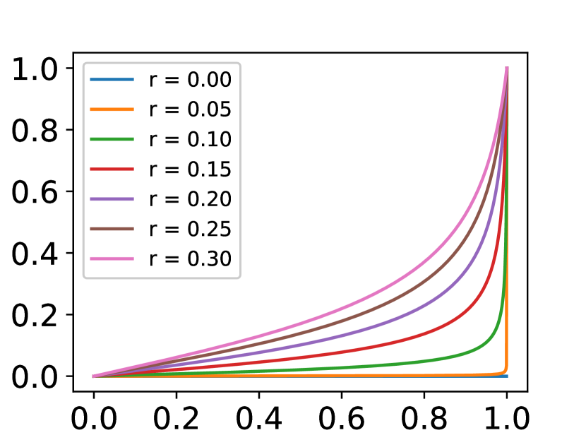
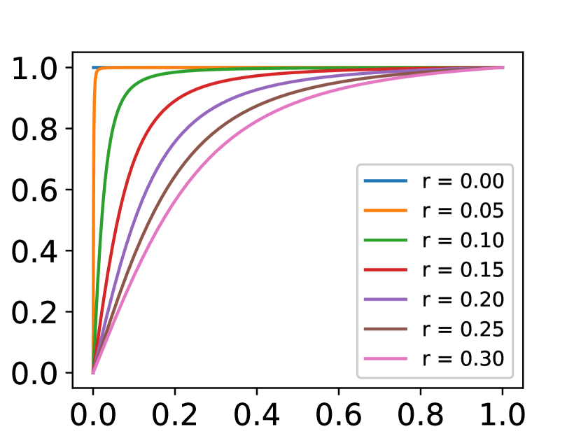
Table 1 illustrate the minimum requirement of for an individual to improve under different , and the best attainable profile for individuals with initial similarity . We illustrate them in Fig. 7.
Discussions of intervention strategies in real applications.
Table 1 further suggest effective strategies that encourage individuals to improve their qualifications, i.e., more individuals are incentivized to improve if (i) the decision-maker’s acceptance threshold is lower; or (ii) the time it takes for individuals to succeed after investments is shorter. Examples of both strategies in real applications are as follows.
-
1.
Lower acceptance threshold in hiring: Instead of directly recruiting the qualified candidates, companies first lower the standard by offering internship opportunities to encourage applicants to improve, and then offer full-time positions. This two-stage hiring process widens the candidate pool and incentivizes more people to improve.
-
2.
Lower discounting factor in college admission: Instead of directly rejecting the unqualified high school graduates, universities incentivize them by issuing conditional transfer offers. Once these students meet certain requirements, they get admitted. The conditional acceptances encourage more students to improve by lowering the time it takes for them to receive reward.
Meanwhile, Table 1 also reveals that setting short-term goals will be effective to incentivize individuals to improve. For instance, teachers may set up several quizzes to break down the grade and make students more motivated to improve.
Appendix E Illustration of Thm. 5.1
| Detection probability | |||||||
|---|---|---|---|---|---|---|---|
| 0 | 0.1 | 0.2 | 0.3 | 0.4 | 0.5 | ||
Thm. 5.1 identifies conditions under which manipulation (or improvement) is preferred by individuals over the other. As mentioned in Section 5, the specific values of , , , in Thm. 5.1 depend on , , and we can empirically find , , , and verify the theorem, as illustrated in Figure 8 and Table 2. Specifically, the left plot in Figure 8 shows as functions of initial similarity under different detection probability . Because individuals only prefer to manipulate if , the plot shows the values of , , , in Thm. 5.1. The right plot shows threshold under different pairs of , and it shows that increases as increases. Table 2 shows ranges of initial similarity under different detection probability , acceptance threshold , and discounting factor .
Appendix F Additional Experiments
Exam Score Data
Just as Sec. 7 mentions, we acquire the exam score data Kimmons (2012), preprocess the data and fit beta distributions for both males and females. The fitted distribution and real distribution are shown in Fig. 9.
FICO Score Data
Just as Sec. 7 mentions, we fit beta distributions for FICO Score Hardt et al. (2016b), and obtain four distributions for different racial groups as shown in Fig. 10.
Additional Results for FICO Data
Besides Caucasian and African American mentioned in Sec. 7, for Asians and Hispanic, we also compute the optimal decision threshold and corresponding total improvement under different . As shown in Fig. 11, always decreases with and the total amount of improvement decreases. If comparing Asians and Hispanics, we observe that Hispanics have lower thresholds but larger improvements. For settings with both manipulation and improvement (Fig. 11), it seems that a larger (resp. smaller) proportion of Asians tend to manipulate than African Americans under . More importantly, the optimal thresholds reveal larger amounts of improvement for Hispanics, suggesting that the decision-maker’s policy in Sec. 4 is beneficial for the disadvantaged group.
Appendix G Estimating the discounting factor in Sec.4
We can estimate the discounting factor if given an experimental population. The decision-maker can publish an arbitrary threshold and observe the lowest score among all individuals who change their scores, which is . Then the decision-maker can use any expression in Table 1 to estimate . Multiple experiments can make the estimation more robust.
Appendix H Proofs
H.1 Proof Details of Thm. 3.1
To derive , we first take the derivative of (5) with respect to . For simplicity, let and the derivative will not change. Also, let and . Then show the results as follows:
| (13) |
| (14) |
The denominator of is always positive, and the first term of numerator is always negative.
Also, because , . Thus, we have following situations:
1) If , is always positive when . This means is increasing.
Then, noticing that , we know is always negative when . This means is monotonically decreasing. Also, when , . This ensures is always non-positive and individuals will never choose to invest any effort.
2) If , is first positive, then negative when . Also, if plugging into (13), we know . These facts reveal that is firstly increasing from a negative number and then decreasing to a negative number. And there must exist a unique maximum point when , should satisfy:
| (15) |
| (16) |
Then take the derivative of :
| (17) |
(17) shows is decreasing. Also, noticing that and , we know there must exist a as the root of . We can explicitly solve .
Thus, we now know that when , . With the plausible domain of and (15), we would know: When , and thereby has an extreme large point with value . At this maximum point, (13) equals 0, and (14) is smaller than 0.
Finally, we derive the condition for : Denote as and as , can be simplified to:
| (18) |
Because , for any fixed, and . With the fact that , we know is monotonically decreasing with , so is . Thus, there must exist a threshold , when , . And if , individuals will decide to improve. Then Thm. 3.1 is proved and we can numerically solve the threshold .
Although we believe exponential discounting is general and fits our setting well, we also note that we can still use derivative analysis when the discounting changes (e.g., hyperbolic discounting). Specifically, if denoting the discounted reward as , we would have . Then if taking the derivative we will get . Noticing that is known, then discussing the properties of with different choices of discounting is enough to derive the nature of .
H.2 Proof Details of Thm. 4.1 and Corollary 4.2
H.2.1 Proof of Thm. 4.1
First prove has a maximize :
With the definition of in (7), we already know is continuous. We can first observe that . These hold simply because . Next noticing that for any , holds. This suggests that will reach its maximum point according to the Weierstrass extreme value theorem.
Next, noticing that we can derive that and . Then if it only has one root in , we would know must first increase and then decrease because there is at most one inflection point. Thus, a unique maximum exists.
H.2.2 Proofs of why Uniform distribution has a unique maximized
If only has one root. We know it is first larger than 0, then becomes smaller than 0. Next, according to the Leibniz integral rule, we can get:
Use Lagrange’s Mean Value Theorem, we can write the above equation as:
where is between . Thus, the second term must also be first larger than 0 then smaller than 0. Next, noticing that in uniform distribution and is increasing, the equation will be smaller than 0 when and vice versa. Thus, we prove the result for the uniform distribution.
H.2.3 Proof of Corollary 4.2
We now know . Then according to the expression of , it is true that both and increase with . Thus, when the probability distribution remains unchanged, the root of when increases becomes smaller.
H.3 Proof Details of Thm. 5.1
Denote as . is always negative and monotonically increasing with .
1. Situation when P = 0
According to Sec. 3 and (8), we can write the maximum improvement utility as , and write manipulation utility as .
Then take the derivative of both:
| (19) |
| (20) |
The “" in (19) occurs because is actually a function of , but if we regard at as a constant, the derivative here serves as a lower bound of .
Firstly, we prove when , : when , we know since individuals invest an arbitrarily small effort to immediately qualified. However, according to Sec. H.1, should let . This inequality will give us the bound of : . With this bound, we can plug into (19), and know , and is larger than a constant because of the bound. Therefore, . Then according to (20), when , . Since is always positive, when , we prove that . Meanwhile, when , . This means when , .
Secondly, when : and . So when .
Thus. there must be an intersection between and . Then noticing that if we increase , is always decreasing to converge to function , while always holds. This suggests when is sufficiently close to 1, we can guarantee the first intersection of and occurs arbitrarily close to 1, meaning this first intersection is the only intersection.
Let the only intersection be , we prove situation 1. The shapes of and are illustrated in Fig. 12.
2. Situation when P 0
From (8): when , . However, at this time . This demonstrates must exist.
When , according to situation 1 and the continuity of with respect to , must exist. However, when , is always negative, making does not exist.
Thus, there must exist a threshold , when , exist. Otherwise, is always true.

H.4 Proof Details of Thm. 6.2
First let us prove following two lemmas:
Lemma H.1.
For any initial qualification score , There exists a , when ), . Let be the only root of within , then is given by:
| (21) |
Proof
According to Thm. 6.1, and . We can get following expression:
| (22) |
Firstly, when , . Thus, when , .
Except the above situation, We can regard (22) as a quadratic function of and solve the two roots:
| (23) |
We then prove a claim that when , is either larger than 1 or smaller than 0:
1) When , the denominator of (23) is negative, while the numerator is always positive. Thus, (23) is negative.
2) When :
| (24) |
Thus, only has one root within . Also from (22) we know when , and when , . With these facts we immediately know: When , . Otherwise, . In fact, besides the exception , there are only two possibilities of the shape of as shown in Fig. 13. Because and are both non-negative, the relationship of the square must be the same for their values.
Then if we define as:
| (25) |
Then when . Proved.
Lemma H.2.
For any individual with initial qualification score and the admission threshold , there must exist a to let there exists a ,
Proof. If we let be and recall that , we would have .
For any there exists , when , .
So we can just let be an arbitrary point and we can get the corresponding , then we can only let satisfy:
| (26) |
Then we find the plausible . Proved.
Proof of Thm. 6.2
According to Lemma H.1, when , , so the convergence speed of the individual to under forgetting mechanism will be faster than the convergence speed of the individual to without forgetting mechanism, so that the reward under forgetting mechanism is discounting less. Meanwhile, according to Lemma H.2, there exists a where . Combine them together, and Thm. 6.2 is proved.
H.5 Proof of Thm. B.1
Then consider . When , The expression is , demonstrating the convergence rate is linear. Note that this expression is decreasing as decreases, so the convergence rate in our model is always slower than linear. Next, consider the general expression and . Let which is larger than , and which is larger than . We slightly abuse the definition of to let it be an integer. Then the expression becomes .
Then for any we can bound this expression. Basically, we already know . Noticing that when , it is just equal to erase some terms of this expression. We can utilize this fact to get the lower bound and upper bound:
-
1.
Lower bound: consider the following sets of expressions and each set consists of terms: , …, . Then each of the expressions are smaller than . Denote as , we will have , so the convergence rate is smaller than
-
2.
Upper bound: consider the following sets of expressions and each set consists of terms: , …, . Then each of the expressions are larger than . Denote as , we will have , so the convergence rate is larger than
Thus, take the limit and apply the Sandwich Theorem, the convergence rate is .