On computational complexity and average-case hardness of shallow-depth boson sampling
Abstract
Boson sampling, a computational task believed to be classically hard to simulate, is expected to hold promise for demonstrating quantum computational advantage using near-term quantum devices. However, noise in experimental implementations poses a significant challenge, potentially rendering boson sampling classically simulable and compromising its classical intractability. Numerous studies have proposed classical algorithms under various noise models that can efficiently simulate boson sampling as noise rates increase with circuit depth. To address this issue particularly related to circuit depth, we explore the viability of achieving quantum computational advantage through boson sampling with shallow-depth linear optical circuits. Specifically, as the average-case hardness of estimating output probabilities of boson sampling is a crucial ingredient in demonstrating its classical intractability, we make progress on establishing the average-case hardness confined to logarithmic-depth regimes. We also obtain the average-case hardness for logarithmic-depth Fock-state boson sampling subject to lossy environments and for the logarithmic-depth Gaussian boson sampling. By providing complexity-theoretical backgrounds for the classical simulation hardness of logarithmic-depth boson sampling, we expect that our findings will mark a crucial step towards a more noise-tolerant demonstration of quantum advantage with shallow-depth boson sampling.
I Introduction
Boson sampling is a computational task that is complexity-theoretically proven to be hard to classically simulate under plausible assumptions [1, 2, 3]. Accordingly, boson sampling has gathered significant attention, as it would possibly play a key role in the experimental demonstration of quantum computational advantage using near-term quantum devices. However, the implementation of boson sampling in experimental settings with near-term quantum devices is inevitably subject to various sources of noise [4, 5, 6, 7]. The problem is that those noises would possibly rule out the classical intractability of boson sampling, and thus potentially hinder the experimental demonstration of quantum advantage with boson sampling. Indeed, both for finite-size near-term experiments and asymptotic limits as system size scales, numerous studies [8, 9, 10, 11, 12, 13, 14, 15, 16, 17, 18, 19] have proposed efficient classical simulation algorithms of boson sampling under various noise models, such as photon loss, partial distinguishability, gaussian noise, etc. Their results indicate that as the noise rate of boson sampler increases, it eventually renders such a noisy sampler classically simulable. Moreover, as the noise is typically accumulated with each circuit depth, the quantum signal for classical intractability exhibits exponential decay with increasing circuit depth. Hence, circuits with polynomially increasing depth with system size would suffer from significantly enlarged noise rates, posing substantial challenges to achieving quantum advantage in such settings.
A viable alternative to preclude the classical simulability due to the inevitable noise is to consider boson sampling with shallow-depth linear optical circuits, where the noise rate can be highly reduced. Specifically, among the shallow-depth regime, our primary focus is on investigating the simulation hardness for depth circuits; the intuition behind investigating logarithmic depth circuits lies in the potential to offer a “sweet-spot” regime for the hardness of boson sampling. Namely, this depth regime may avoid significant increases in noise rates to prevent classical simulability, while still being sufficiently large to generate quantum correlations and uphold simulation hardness. Despite such intuitive understanding, the hardness argument of boson sampling in this shallow-depth regime, particularly from a complexity-theoretical perspective, has been less studied so far and thus remains widely open. Hence, our goal is to establish the complexity-theoretical foundations of the classical hardness of shallow-depth boson sampling, to suppress the classical simulability by noise in a rigorous manner and obtain a more noise-tolerant demonstration of quantum advantage with boson sampling.
In this work, we investigate the classical simulation hardness of boson sampling in shallow linear optical circuits. Specifically, as the average-case #P-hardness of estimating output probabilities of boson sampling is a crucial ingredient to demonstrate the classical intractability of boson sampling, we make progress on establishing the average-case #P-hardness confined in shallow-depth regimes. Similarly, we obtain the average-case hardness result in the shallow-depth regime for the Gaussian boson sampling scheme. Finally, since noise is our main motivation for investigating shallow-depth boson sampling, we generalize our average-case hardness result to noisy boson sampling subject to a photon loss channel.
To avoid confusion, we note that the allowed imprecision level of our average-case #P-hardness result is not sufficient to fully demonstrate the classical intractability of boson sampling in shallow-depth regimes. However, to the best of our knowledge, the complexity-theoretical analysis on the average-case hardness of shallow-depth boson sampling has not yet been investigated. Hence, we believe that our hardness result in shallow-depth regimes will provide a first step toward a stronger hardness result and, ultimately, toward the full demonstration of the classical intractability of shallow-depth boson sampling.
I.1 Outlines: average-case hardness of shallow-depth boson sampling
We set our goal as proving the hardness of classical simulation of boson sampling in the shallow-depth regime, specifically for approximate simulation within total variation distance error. Two key ingredients for the current hardness proof of the approximate simulation of boson sampling are average-case #P-hardness of output probability approximation up to sufficiently large additive imprecision , and hiding property. Informally, average-case hardness means that approximating the output probability of boson sampling with high probability over randomly chosen circuits (i.e., on average over circuits) is #P-hard. Here, by choosing random circuit instances that have the hiding property (i.e., symmetric over outcomes), one can reduce the average-case instances for the hardness from circuit instances to outcome instances, which is a crucial step to prove the hardness of approximate simulation within total variation distance error (See Appendix A for more details).
Most of the current theoretical foundations of the average-case hardness of boson sampling rely on global Haar random unitary circuits [1, 2, 3, 20, 21, 22], as they almost satisfy the two conditions described above. Namely, the outcome instances can be effectively hidden by global Haar random unitaries, and approximating the output probability within sufficiently large on average over global Haar random circuit instances is #P-hard under some conjectures. However, the problem is that implementing global Haar random unitary requires at least polynomial circuit depth (e.g., see [23, 24]), and thus not implementable in sub-polynomial circuit depths. Accordingly, the hardness results built upon global Haar random unitaries cannot be directly applied to the shallow-depth boson sampling we are interested in, necessitating a different approach from them.
Another problem is that there already exist efficient classical algorithms that can approximately simulate shallow-depth boson sampling in certain circumstances, which directly rule out the classical simulation hardness in shallow-depth for such cases. Although exact simulation of boson sampling is classically hard even for constant depth circuits [25], approximate simulation is easy for 1 local log depth circuits [26, 27] and also for more general dimension local circuits under some constraints [28, 29]. Specifically, according to their results, if we use circuits composed of only geometrically local gates, at least polynomial circuit depth is required for a sufficiently large correlation to obtain the approximate simulation hardness. Those results indicate that we cannot expect the hardness results in the most general case of shallow-depth circuits composed of local gates only.
To deal with those problems we take the following approach: first, we consider shallow linear optical circuit architectures composed of geometrically non-local gates. In fact, implementation of non-local gates is promising for near-term experimental settings; for example, experiments of linear optical systems based on trapped ions [30, 31] and photonic architecture [6] implemented long-range interactions. Also, since we cannot implement global Haar random unitary within shallow-depth regime, we instead employ local random circuit ensemble for random circuit instances in shallow circuit architecture, inspired by the hardness results of random circuit sampling [32, 33, 21, 34, 35]. Here, local random distribution in this context means that each gate composing the circuit is independently chosen Haar random gate; we note that recent experimental setups of boson sampling [4, 5, 6, 7] also follow such circuit distribution, but with geometrically local architectures.
However, local random distribution poses a subsequent challenge toward the average-case hardness of shallow-depth boson sampling, that is, the absence of the hiding property. Since the output symmetry of boson sampling over local random circuit distribution is not evident, the random outcome instances cannot be efficiently hidden by random circuit instances. This means that even if we find the average-case hardness over randomly chosen circuits for a fixed outcome, it still does not lead to the classical simulation hardness grounded in Stockmeyer’s reduction from the average-case approximation over randomly chosen outcomes [1]. To address this issue, we prove the average-case hardness over both the randomly chosen outcome and randomly chosen circuit, by establishing a worst-to-average-case reduction for both outcome and circuit instances. Specifically, our reduction process is composed of two steps: from a given fixed outcome to a randomly chosen collision-free outcome, and from a worst-case circuit to a randomly chosen circuit over local random circuit distribution.
To sum up, we show the average-case hardness over outcomes and circuit instances for shallow circuit architectures composed of non-local gates and employing the local random circuit ensemble. We informally present here our average-case hardness result of boson sampling in the logarithmic depth regime, for photon number and mode number with .
Theorem 1 (Informal).
There exists a -depth linear optical circuit architecture such that approximating output probability of boson sampling within additive error with high probability over randomly chosen circuits in the circuit architecture for high probability over randomly chosen collision-free outcomes is #-hard under reduction.
Also, since our average-case hardness result considers both the random outcomes and random circuits due to the absence of the hiding property, it is not straightforward to show the classical simulation hardness of shallow-depth boson sampling as in the original boson sampling proposal [1]. Accordingly, we show how our average-case hardness result over both the randomly chosen outcomes and circuits leads to the classical simulation hardness argument. This implies that improving the additive imprecision for our average-case hardness result is the only remaining problem for the fully theoretically guaranteed classical intractability of shallow-depth boson sampling.
Theorem 2 (Informal).
Now we provide an outline of our results, which is depicted in Fig. 1. We first define in Sec. II a shallow-depth circuit architecture composed of non-local gates, which we will use throughout our results. Next, in Sec. III we prove the worst-case #P-hardness of approximating output probability of a fixed outcome of boson sampling, for any circuit in the shallow circuit architecture previously defined. In Sec. IV we prove the average-case #P-hardness of approximating output probability for randomly chosen outcome and randomly chosen circuit in the shallow circuit architecture, by establishing worst-to-average-case reduction. We prove in Sec. V how our average-case hardness results over both the random outcomes and random circuits lead to the classical simulation hardness. We also extend our average-case hardness result to the Gaussian boson sampling scheme in Sec. VI, and to the lossy boson sampling subject to photon loss channels in Sec. VII. In Sec. VIII, we conclude with several remarks.

II Notations
Let us define the total mode number as , where we set as a power of 2 for simplicity. We set the output photon number polynomially related to as , for a constant and satisfying . We use the notation as an -dimensional output configuration vector for the collision-free outcome, such that each element of denotes photon number in th mode. Namely, where each with , so that the number of possible configurations of is . We define as an output probability of a linear optical circuit (unitary) matrix for the outcome from a predefined input configuration . For collision-free input and output, can be represented as [1]
| (1) |
where is a by matrix obtained by taking copies of the th row and copies of the th column of the matrix .
We note that an -mode linear optical circuit can be represented by an by unitary matrix in U which unitarily transforms mode operators. Specifically, we can represent a single-mode gate (i.e., a phase shifter) as a U matrix to the mode, and a two-mode gate (i.e., a beam splitter) as a U matrix along the modes. Also, the parallel application of gates can be represented as a unitary matrix with a block matrix form, and the serial application of gates can be represented as matrix multiplication of the unitary matrices. Accordingly, throughout this work, we will interchangeably use the terminology ‘(linear optical) circuit’ and ‘(unitary) matrix’.
We first define the linear optical circuit architecture, for a more rigorous analysis of the hardness proof.
Definition 1 (Linear optical circuit architecture).
The linear optical circuit architecture is a linear optical circuit with fixed type (i.e., single- or two-mode) and fixed location of gates, where the coefficients of each gate are not specified. If the coefficients of each gate are specified with unitary matrices (in or ), then the circuit and the corresponding unitary matrix are specified.
For the shallow-depth circuit architecture, specifically in logarithmic depth, we define the shallow linear optical circuit architecture of circuit depth , using the convention used in [36, 37].
Definition 2.
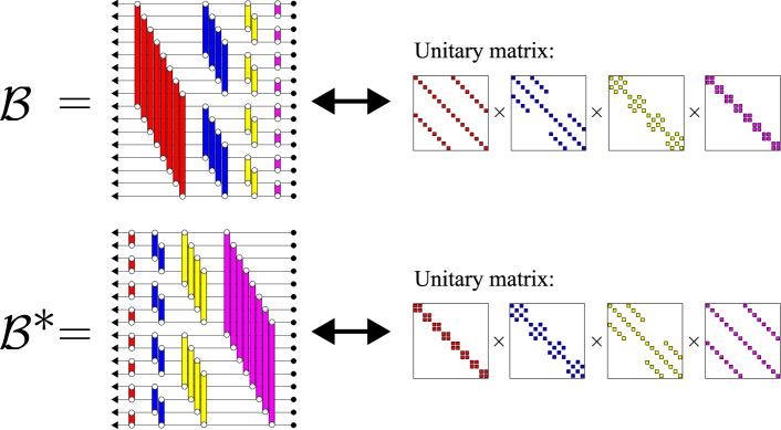
We define butterfly circuit architecture as follows: for each layer of the circuit architecture, allocate two-mode gate between mode number and , for all and . Also, we define inverse butterfly circuit architecture as a butterfly circuit architecture with the inverse sequence of gate application along the depth.
We illustrate in Fig. 2 the circuit architecture and , and the form of their corresponding unitary matrix. Next, we define the Kaleidoscope circuit architecture proposed in [36], using the butterfly circuit architecture defined above.
Definition 3.
We define Kaleidoscope circuit architecture as a serial application of over . We also define -Kaleidoscope circuit architecture as a repeat of the Kaleidoscope circuit architecture, with repetition number .
Here, the circuit depth of -Kaleidoscope architecture is , which is indeed a logarithmic depth in for . Throughout this paper, we will focus on the -Kaleidoscope circuit architecture with to demonstrate the hardness results for shallow-depth circuits. One motivation for employing this linear optical circuit architecture is that it enjoys a useful property that is crucial for our analysis; Ref. [36] shows that for a power of , any mode permutation circuit can be implemented within .
Lemma 1 (Dao et al [36]).
Let be an arbitrary permutation matrix with a power of 2. Then can be efficiently implemented in using two-mode permutation gates, i.e., and .
III Worst-case hardness of output probability estimation
In this section, we find the worst-case #P-hardness of output probability estimation of shallow-depth linear optical circuits in , for a fixed input and output within a certain additive imprecision. Our worst-case hardness result for the shallow circuit architecture can be represented as follows.
Theorem 3 (Worst-case hardness).
For , approximating the output probability to within additive error for any over linear optical circuit architecture is #-hard in the worst case.
We briefly sketch the proof of our worst-case hardness result for the shallow circuit architecture . The proof is based on the result by [25], which showed the simulation hardness of exact boson sampling with constant depth linear optical circuits. Specifically, there exist constant-depth linear optical circuits that can simulate an arbitrary given quantum circuit using post-selection. Also, those constant depth circuits can be embedded in our circuit architecture . Hence, additively approximating the output probability of any quantum circuit can be reduced to additively approximating the output probability of any circuit in , with imprecision blowup up to the inverse of post-selection probability. Using the fact that the additive approximation of any quantum circuit is #P-hard for certain additive imprecision [34], we can obtain the worst-case hardness of our shallow circuit architecture .
IV Average-case hardness of output probability estimation
In this section, we prove the average-case #P-hardness of approximating output probabilities of shallow-depth boson sampling within a certain additive imprecision. We focus on -Kaleidoscope circuit architecture with , where the gate number for such architecture is . From the result of Theorem 3, has the worst-case hardness of output probability approximation, for .
Our main strategy for the average-case hardness is the establishment of the worst-to-average-case reduction, using the result of Theorem 3. In other words, we prove that if we can well-approximate the output probability , we can also well-approximate the worst-case output probability in Theorem 3. Here, our average-case approximation regards both the randomly chosen outcome and the randomly chosen circuit, since we cannot rely on the hiding property that enables us to fix the outcome. For this reason, we define both the random circuit ensemble and the random outcome ensemble as follows.
Definition 4 (Random circuit ensemble).
Let be the circuit architecture with number of gates. We define as the distribution over circuits with architecture , whose gates are independently distributed local Haar random matrices .
Definition 5 (Random collision-free outcome ensemble).
We define as the uniform distribution over collision-free outcomes of boson sampling with modes and photons. Each outcome is an -dimensional output configuration vector for the collision-free outcome, such that where each with .
Using the definitions above, we first state our result on the average-case hardness over the outcome and circuit instances, for shallow-depth linear optical circuit architecture with .
Theorem 4 (Average-case hardness).
The following problem is #-hard under a reduction: for any constant with , on input a random circuit with and a random outcome , compute the output probability within additive imprecision , with probability at least over the choice of for at least over the choice of .
In the following, we sketch the proof of Theorem 4, by briefly describing the worst-to-average-case reduction process; we leave in Appendix C a detailed proof of Theorem 4. Since our average-case hardness regards both outcomes and circuits, we first describe how to effectively fix the outcome, so that the remaining problem is to establish worst-to-average-case reduction for fixed output probability over random circuit instances. To do so, our strategy is to randomly permute both a given worst-case circuit and a given fixed outcome. That is, we sample random -mode permutation and permute the worst-case circuit and the fixed outcome equally with , where the permuted outcome now follows the random outcome ensemble . Then the fixed worst-case output probability is equal to , and thus we can obtain the value by inferring via worst-to-average-case reduction over random circuit instances. Here, now becomes a new worst-case output probability, such that the revised worst-case circuit is the randomly permuted circuit , and the revised fixed outcome is the randomly chosen outcome from .
To establish the worst-to-average-case reduction from the revised worst-case circuit to the average-case circuit over for a fixed outcome , our strategy is to perturb the circuit from with the given worst-case circuit parameterized by a constant . That is, corresponds to the average-case distribution and corresponds to the worst-case circuit . Specifically, we choose a perturbation method such that for small enough , the success probability of average-case approximation over perturbed random circuits would not have largely deviated from the ideal case (), and as grows, the perturbed circuit converges to the worst-case circuit . Using such perturbation method and as long as values are small enough, one can obtain the average-case approximate output probability values with high probability over perturbed circuits, parameterized by different values of . Also, we can expect that those average-case values contain some information about the worst-case value , depending on the perturbation method and the values of . Assuming that worst-case value can be inferred using the average-case values with small values of , one can finally infer the worst-case value , within a certain imprecision determined by the average-case approximation imprecision and the method for the inference.
Therefore, it is crucial to choose a proper perturbation method to establish the worst-to-average-case reduction successfully. Throughout this work, we use the Cayley path for the perturbation, which was employed in Refs. [33, 21, 34] for the hardness proposals of the random circuit sampling.
Definition 6 (Cayley transform [33]).
The Cayley transform of an by unitary matrix parameterized by is a unitary matrix defined as
| (2) |
where is the by identity matrix. Also, for the diagonalization of the by unitary matrix , with unitary matrix and diagonal matrix , the equivalent form of the Cayley transform is
| (3) |
where
| (4) | |||
| (5) |
Using the Cayley transform defined above, we now define the perturbed random circuit distribution.
Definition 7 (Perturbed random circuit ensemble).
Let be the circuit architecture with number of gates. For the given circuit in with gates , the circuit is defined with each gate of replaced by , where each is a Cayley transform of independently distributed local Haar random gate parameterized by . We define as the distribution for such . Here, the distribution of the is , and .
Before proceeding, we should make sure that the success probability of average-case approximation over circuits is still large enough after the perturbation, to establish the reduction process successfully. This is evident in the case that the total variation distance over circuits induced by the perturbation is small enough, as the success probability over circuits perturbs by, at most, the total variation distance.
In fact, Ref. [33] proved that total variation distance between and is small for comparably small perturbation .
Lemma 2 (Movassagh [33]).
Let be the circuit architecture with number of gates. For and for any circuit in , total variation distance between and is .
Therefore, by using small , one can upper-bound the total variation distance by an arbitrarily small constant, which implies that the success probability of average-case approximation over circuits also perturbs by at most a small constant.
For the worst-to-average-case reduction, we first sample a random circuit with and worst-case circuit . Using with the same random seed but with different values of satisfying , we obtain the average-case approximation of the output probability for each , which may enable us to infer the worst-case output probability value .
To investigate the feasibility of the inference of the worst-case value, we examine the behavior of the function characterized by the parameter . Using Definition 6, we find that can be represented as a low-degree rational function in .
Lemma 3.
Let be the -Kaleidoscope circuit architecture with number of gates, and for any in . Then for any outcome , the output probability can be represented as a degree rational funtion in .
Proof.
For given circuit unitary matrix with composed of gates, one can decompose with product of unitary matrices, such that each matrix element of can be represented as
| (6) |
where each denotes an -dimensional unitary matrix, with a single gate unitary matrix applied to the modes participating in the gate and identity for the rest of the modes. For example, if the th gate is a two-mode gate between the first two modes, is a block diagonal matrix of and identity matrix, namely, .
For circuit architecture which is composed of only two-mode gates, matrix elements of can be represented as degree rational functions in , where the common denominator for the elements is given by , defined in Eq. (4) but with index appended for th random gate . Using reduction to the common denominator for all of the gates, can be represented as rational function in with the common denominator ; note that it does not change with the indices .
From Eq. (1), the output probability has the form of
| (7) | ||||
where is an input configuration vector, and is -mode permutation group. One can easily check that the common denominator for is , and it does not change with permutation . Let us define , which is a degree polynomial in . Then serves as the common denominator for the output probability. Hence, the output probability can be represented as , with also a degree polynomial in . ∎
We are now ready to turn to the proof of Theorem 4, i.e., the average-case hardness of the shallow-depth boson sampling. We prove that for high probability over , well-approximating output probability with high probability over for the shallow-depth architecture is #P-hard under a reduction.
V Average-case hardness implies classical simulation hardness
As we have previously discussed, since our average-case hardness result considers both the random outcomes and random circuits, it is not straightforward to show the classical simulation hardness of shallow-depth boson sampling as in the original boson sampling proposal [1]. Therefore, in this section, we provide a self-contained analysis of how our average-case hardness result leads to the classical simulation hardness arguments of shallow-depth boson sampling. Specifically, we show that if the allowed additive error in Theorem 4 for the hardness is improved to a certain imprecision level, an efficient classical algorithm that can approximately simulate the shallow-depth boson sampling is unlikely to exist. This emphasizes that improving the imprecision level of the average-case hardness in Theorem 4 is a crucial step for the classical intractability of shallow-depth boson sampling.
Definition 8 (Approximate boson sampler).
Approximate boson sampler is a classical randomized algorithm that takes input linear optical circuit and outputs a sample from the output distribution such that
| (8) |
where is the ideal output distribution of the circuit and represents total variation distance.
Given the total variation distance error, the above approximate sampler can have an arbitrarily large additive error for a fixed output probability. Nevertheless, it still has a comparably small additive error for most of the output probabilities due to Markov’s inequality. Accordingly, finding the average-case solution of the output probability of the ideal sampler over randomly chosen collision-free outcome , up to a certain additive imprecision, is in complexity class by Stockmeyer’s theorem [38].
Lemma 4 (Average-case approximation [1]).
If there exists an approximate boson sampler with total variation distance , then for any linear optical circuit , the following problem is in : find the average-case approximate solution of , which satisfies
| (9) |
where is over all collision-free outcomes, and are the fixed error parameters satisfying .
We leave the proof of Lemma 4 in Appendix D for a more self-contained analysis. The complexity is known to be inside the finite level of PH, i.e., . Also, by Toda’s theorem [39], PH problems can be solved given the ability to solve any #P problem, i.e., . If finding the average-case solution of output probabilities of sampler is #P-hard, then . Therefore, if an efficient classical algorithm exists that can simulate , then which implies the collapse of PH. Consequently, under the assumption of the non-collapse of the PH, there is no efficient classical algorithm capable of simulating .
Based on the above arguments, we show that for the case that allowed additive imprecision of Theorem 4 for the hardness can be improved, then it is classically hard to simulate shallow-depth boson sampling within a constant total variation distance.
Theorem 5.
Suppose that the allowed additive imprecision for the problem in Theorem 4 to be #-hard can be improved to . Then the efficient classical simulation of approximate boson sampler with respect to circuits from the shallow architecture implies the collapse of .
Proof.
We establish a reduction from the problem in Theorem 4 with allowed additive error to the problem in Lemma 4. Let be an oracle that solves the problem in Lemma 4, i.e., on input a circuit and a randomly chosen collision-free outcome , outputs an estimate of output probability up to additive imprecision , with probability at least over outcomes for any circuit. For convenience, we refer to the outcomes which estimates with error larger than as bad outcomes, such that the portion of bad outcomes over possible collision-free outcomes is at most for any circuit.
For the randomly chosen circuit input, bad outcomes can vary with the circuit instances, as the sampler has the freedom to choose its error distribution according to the input circuit. However, no matter how the bad outcomes vary with circuit instances, succeeds at least fraction over circuit instances for at least fraction of the outcomes, for any satisfying . Otherwise, the failure probability over outcomes and circuits would exceed , which contradicts the proposition that the success probability of is at least over randomly chosen outcomes and circuits. As the above argument holds for any random circuit families, we choose the random circuit distribution as with the shallow architecture .
To sum up, on input a random circuit and a random outcome , the oracle estimates the output probability up to imprecision , with probability at least over the choice of for at least over the choice of . Here, the additive imprecision can be bounded as
| (10) | ||||
| (11) |
for constant and so as , where we used the relation with a constant and . By setting and small constant satisfying , we can solve the problem in Theorem 4 up to additive imprecision using the oracle . Hence, assuming that the above problem is #P-hard under reduction, we can obtain the complexity-theoretical relation , which implies the collapse of PH if with respect to shallow-depth circuit architecture can be done in classical polynomial time. This completes the proof. ∎
VI Classical simulation hardness of shallow-depth Gaussian boson sampling
In this section, we show that our hardness results of the shallow-depth boson sampling can be generalized to the Gaussian boson sampling scheme [2]. Our specific setup for the Gaussian boson sampling is as follows. Let the total mode number of the circuit be a power of 2, and now the input state is an product of single-mode squeezed vacuum (SMSV) state with equal squeezing parameter and equal squeezing direction. Also, let us define the output mean photon number as an integer (i.e., ) where and are polynomially related as for a constant and . We define as an output probability of the Gaussian boson sampling, for an photon outcome from an mode linear optical circuit matrix on input SMSV states. For collision-free outcome , can be expressed as [2]
| (12) |
where is an -mode Fock state corresponding to the outcome , is a unitary operator corresponding to the circuit , and is an by matrix obtained by taking copies of the th row and column of the matrix .
Using the above settings, we first prove the worst-case hardness of Gaussian boson sampling for a fixed outcome , with the shallow-depth circuit architecture .
Theorem 6.
Approximating the output probability of Gaussian boson sampling to within additive error for any over linear optical circuit architecture is #-hard in the worst case.
Proof.
We establish a reduction from the worst-case hardness of boson sampling in Theorem 3 to the problem in Theorem 6. Let be the output probability of a fixed input and output of boson sampling in Theorem 3, for mode number , photon number , and the circuit in mode circuit architecture . In the following, we show that can be efficiently reduced to the output probability of Gaussian boson sampling, for mode number and mean photon number , with output and circuit determined by and each.
Our strategy is to employ the scheme in Ref. [40], which used product of equally squeezed two-mode squeezed vacuum (TMSV) state as an input state to perform mode boson sampling task. Specifically, a single TMSV state with squeezing parameter can be represented as
| (13) |
and thus product of the TMSV state is
| (14) | ||||
where the summation of is over all possible configurations of Fock state with a total mode and photon.
For each mode in the given mode circuit , one-half of the TMSV state (i.e., subscript (2) in Eq. (14)) is input into it, and the other half of each state (i.e., subscript (1) in Eq. (14)) is sent directly to a photon counter. By setting each and as a total mode and total photon Fock state, the output probability can be represented as
| (15) |
which is the output probability of mode and photon boson sampling in circuit , with an additional multiplicative factor.
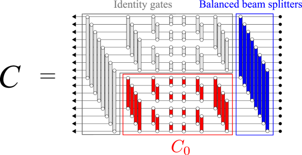
Note that two mode architecture can be embedded in the middle of an mode architecture. Accordingly, we define a circuit in mode by embedding the given mode circuit in one side of , setting gates located right in front of the input ports as balanced beam splitters, and setting the remaining gates as identity gates; we leave in Fig. 3 an illustration of mode circuit for more clarity. Here, the input SMSV states with squeezing parameter combined with the balanced beam splitters at the front becomes TMSV states with squeezing parameter . Therefore, our overall setup exactly follows the scheme in Ref. [40], such that the first mode is the photon counter sector to determine the input configuration of boson sampling, and the last mode is to simulate the boson sampling for the given circuit .
We also define an -dimensional vector as a serial concatenation of two vectors, so that represents photon outcome over modes. Then the output probabilities and are related as
| (16) | ||||
Hence, approximating the output probability can be reduced to approximating the output probability of Gaussian boson sampling, with a blowup in the additive imprecision. The size of the additive imprecision blowup is
| (17) |
using the relation and . Since the allowed additive error for the worst-case hardness of is , the allowed additive error for the reduction is = . This completes the proof. ∎
Using the results of Theorem 6 and the previous proof of the average-case hardness of boson sampling in Theorem 4, it is straightforward to find the average-case hardness of Gaussian boson sampling, for randomly chosen photon outcomes and randomly chosen circuits in shallow-depth architecture .
Theorem 7.
The following problem is #-hard under a reduction: for any constant with , on input a random circuit with and a random outcome , compute the output probability of Gaussian boson sampling within additive imprecision , with probability at least over the choice of for at least over the choice of .
Proof.
The procedure is the same as the proof of Theorem 4, namely, establishing a worst-to-average-case reduction from the problem in Theorem 6 to the problem in Theorem 7. The only different part for the Gaussian boson sampling case is the functional form of the output probability parameterized by . Hence, we show that can also be represented as a degree rational function in , the same degree as the boson sampling case in Lemma 3.
From Eq. (12), the output probability has the form of
| (18) | ||||
where is along all possible perfect matching permutations over modes. From the proof of Lemma 3, using reduction to the common denominator for all of the gates, can be represented as rational function in with the common denominator . Using this fact, one can easily check that can be represented as rational function in , with the common denominator which does not change with . Therefore, the output probability can be represented as , with each and a degree polynomial function in .
VII Extension of hardness results for lossy environments
In this section, we generalize our hardness results for environments, namely, shallow-depth linear optical circuits suffering from photon loss channels after each gate implementation. The reason we consider such a noise channel is that photon loss is indeed a major source of error in optical systems [4, 5, 6, 7]. Also, photon loss ruins the classical intractability of boson sampling, as there exist many efficient classical algorithms that can simulate lossy boson sampling within a constant total variation distance [12, 13, 14]. Therefore, we mainly deal with the photon loss error here; our goal is to provide evidence for the hardness of the approximate simulation of boson sampling in lossy shallow circuits within total variation distance error. For simplicity, we do not consider any photon gain error here, such as thermal radiation noise subjected to the circuits.
To proceed, we start with a brief review of the results presented by Ref. [41], which shows the hardness of simulating noisy quantum circuits. Specifically, one can simulate a noiseless circuit using a larger noisy circuit up to the desired imprecision, by establishing error-detecting code in the noisy circuit and post-selecting null syndrome measurements. Therefore, given the probability to post-select the no-error syndromes, one can approximate the output probability of the noiseless circuit from the output probability of the noisy circuit. Based on this argument, Ref. [21] demonstrates the average-case hardness of approximating output probabilities of noisy quantum circuits, under some plausible assumptions of the noise model. This result gives evidence of the approximate simulation hardness of noisy quantum circuits, within total variation distance error.
The main strategy of the above hardness results is approximating ideal output probabilities by post-selecting error-free results from noisy circuits. Here, we can directly apply their strategy to our case, i.e., lossy shallow-depth linear optical circuits. The crucial observation is that considering photon loss error on boson sampling, the error syndrome is the output photon number . Specifically, if the output photon number is the same as the input photon number, this implies that no loss occurred throughout the circuit. Therefore, by post-selecting the event that the measured output photon number is the same as the input photon number, we can infer ideal output probabilities.
For a more detailed analysis, we set the loss model as follows. Let the photon loss model be local and stochastic. Specifically, is a set of loss channels , such that after each unitary gate is applied, loss channel acts on each mode participated in the unitary gate. Hence, the number of loss channels is for gate number in a given circuit architecture. We can decompose each noise channel as follows:
| (19) |
where is identity, is an CPTP map representing photon loss, and is a loss rate for each channel satisfying for a constant . The validity of such modeling for photon loss channel is represented in [12, 3].
To simplify, we assume that we know each error rate for all , and the noise model is fixed so that it does not change with random circuit instances. Then we can obtain the hardness of approximating output probabilities of lossy shallow circuits, from our previous hardness proposals. To do so, let be the output probability of photon outcome from a mode linear optical circuit which undergoes loss model we set. By post-selecting ‘no loss event’, which can be accomplished by counting the output photon number, the ideal output probability can be inferred from by
| (20) |
From Eq. (19), the probability of ‘no loss event’ is , which can be efficiently calculated. This implies that approximating can be reduced from approximating , with at most blowup in the additive imprecision.
Given Eq. (20), we can repeat the same steps from the previous hardness arguments, for the lossy shallow-depth boson sampling; the only difference is the imprecision blowup by . For our shallow-depth architecture , the gate number is , so the size of imprecision blowup is in our case. Such imprecision blowup does not affect the allowed additive accuracy for our average-case hardness result. Based on the arguments so far, the following corollary is straightforward.
Corollary 1.
Suppose we have the photon loss model with each loss rate for a constant . Then the following problem is #-hard under a reduction: for any constant with , on input a random circuit with and a random outcome , compute the lossy output probability within additive imprecision , with probability at least over the choice of for at least over the choice of .
We remark that for our noise model, the imprecision blowup grows exponentially with the gate number . Therefore, shallow-depth circuits can be more advantageous in this perspective, since they are likely to have less gate number and thus have small imprecision blowup. For example, the current hardness results are based on by submatrices of -dimensional Haar random unitaries, and the implementation of such matrices requires gate number . This arouses the imprecision blowup at least , which restricts the allowed additive error for the average-case hardness at most .
VIII Concluding remarks
Here we provide a few remarks about our overall results and related open questions.
1. Our result demonstrates the average-case hardness for additive imprecision . Indeed, there still remains a gap to the desired additive imprecision for the simulation hardness in Theorem 5. Hence, closing this gap would be an ultimate challenge to the full achievement of classical intractability; more advanced proof techniques are required to reduce this gap. Here, one can take the following approach: finite-size numerical experiments suggest that the output distributions of local random circuits in the butterfly circuit architecture (Definition 2) are close enough to those of global Haar random circuits [37]. Accordingly, if one can analytically prove that the distance between those output distributions is close enough, we can directly obtain a better imprecision level by results in [21, 3, 22], which employed the global Haar random circuits.
Another possible approach for reducing the imprecision gap is to perturb a random circuit matrix in a different way from the Cayley transform (Definition 6), i.e., as depicted in [22]. Specifically, instead of perturbing each random gate, one can perturb a submatrix of our random circuit matrix with a worst-case matrix as for . Here, a degree of polynomial is , which is lower than ours derived by the Cayley transform. Therefore, if one can prove that is distributed similarly to for small , we expect that we can also obtain a better imprecision level by using the same interpolation method. However, the above approach requires one to figure out a global circuit distribution generated by the convolution of local circuit distributions. Although we believe that this problem can be resolved using techniques from random matrix theories, we have not yet developed a complete analysis. Hence, we leave it as an open question.
2. Another important challenge that should be addressed is to find the classical simulation hardness of noisy boson sampling, for general types of physical noise beyond the photon loss noise model we have dealt with so far. To do so, as described in [41, 21, 3], employing the threshold theorem would be a viable choice for this goal. Specifically, the threshold theorem for general types of noise in boson sampling setups has to be developed. This requires an efficient error detection code for general types of error using linear optical elements, for any multi-mode Fock state or Gaussian state input. However, to the best of our knowledge, such an error detection code does not exist. Hence, constructing this error detection code would be a crucial step toward the hardness of noisy boson sampling, which will contribute to a more noise-tolerant demonstration of quantum advantage with boson sampling. We leave this problem as another open question.
Acknowledgement
We thank Bill Fefferman for insightful discussions. The authors acknowledge support from the National Research Foundation of Korea (NRF) grants funded by the Korean government (Grant Nos. NRF-2023R1A2C1006115, NRF-2022M3K4A1097117, and NRF-2022M3E4A1076099) via the Institute of Applied Physics at Seoul National University, the Institute of Information & Communications Technology Planning & Evaluation (IITP) grant funded by the Korea government (MSIT) (IITP-2021-0-01059 and IITP-20232020-0-01606). B.G. was also supported by the education and training program of the Quantum Information Research Support Center, funded through the National Research Foundation of Korea (NRF) by the Ministry of Science and ICT (MSIT) of the Korean government (No.2021M3H3A1036573).
References
- [1] Scott Aaronson and Alex Arkhipov. The computational complexity of linear optics. In Proceedings of the forty-third annual ACM symposium on Theory of computing, pages 333–342, 2011.
- [2] Craig S Hamilton, Regina Kruse, Linda Sansoni, Sonja Barkhofen, Christine Silberhorn, and Igor Jex. Gaussian boson sampling. Physical review letters, 119(17):170501, 2017.
- [3] Abhinav Deshpande, Arthur Mehta, Trevor Vincent, Nicolás Quesada, Marcel Hinsche, Marios Ioannou, Lars Madsen, Jonathan Lavoie, Haoyu Qi, Jens Eisert, et al. Quantum computational advantage via high-dimensional gaussian boson sampling. Science advances, 8(1):eabi7894, 2022.
- [4] Han-Sen Zhong, Hui Wang, Yu-Hao Deng, Ming-Cheng Chen, Li-Chao Peng, Yi-Han Luo, Jian Qin, Dian Wu, Xing Ding, Yi Hu, et al. Quantum computational advantage using photons. Science, 370(6523):1460–1463, 2020.
- [5] Han-Sen Zhong, Yu-Hao Deng, Jian Qin, Hui Wang, Ming-Cheng Chen, Li-Chao Peng, Yi-Han Luo, Dian Wu, Si-Qiu Gong, Hao Su, et al. Phase-programmable Gaussian boson sampling using stimulated squeezed light. Physical review letters, 127(18):180502, 2021.
- [6] Lars S Madsen, Fabian Laudenbach, Mohsen Falamarzi Askarani, Fabien Rortais, Trevor Vincent, Jacob FF Bulmer, Filippo M Miatto, Leonhard Neuhaus, Lukas G Helt, Matthew J Collins, et al. Quantum computational advantage with a programmable photonic processor. Nature, 606(7912):75–81, 2022.
- [7] Yu-Hao Deng, Yi-Chao Gu, Hua-Liang Liu, Si-Qiu Gong, Hao Su, Zhi-Jiong Zhang, Hao-Yang Tang, Meng-Hao Jia, Jia-Min Xu, Ming-Cheng Chen, et al. Gaussian boson sampling with pseudo-photon-number-resolving detectors and quantum computational advantage. Physical review letters, 131(15):150601, 2023.
- [8] Jelmer Renema, Valery Shchesnovich, and Raul Garcia-Patron. Classical simulability of noisy boson sampling. arXiv preprint arXiv:1809.01953, 2018.
- [9] Jelmer J Renema, Adrian Menssen, William R Clements, Gil Triginer, William S Kolthammer, and Ian A Walmsley. Efficient classical algorithm for boson sampling with partially distinguishable photons. Physical review letters, 120(22):220502, 2018.
- [10] Valery S Shchesnovich. Noise in boson sampling and the threshold of efficient classical simulatability. Physical Review A, 100(1):012340, 2019.
- [11] Alexandra E Moylett, Raúl García-Patrón, Jelmer J Renema, and Peter S Turner. Classically simulating near-term partially-distinguishable and lossy boson sampling. Quantum Science and Technology, 5(1):015001, 2019.
- [12] Michał Oszmaniec and Daniel J Brod. Classical simulation of photonic linear optics with lost particles. New Journal of Physics, 20(9):092002, 2018.
- [13] Raúl García-Patrón, Jelmer J Renema, and Valery Shchesnovich. Simulating boson sampling in lossy architectures. Quantum, 3:169, 2019.
- [14] Haoyu Qi, Daniel J Brod, Nicolás Quesada, and Raúl García-Patrón. Regimes of classical simulability for noisy gaussian boson sampling. Physical review letters, 124(10):100502, 2020.
- [15] Daniel Jost Brod and Michał Oszmaniec. Classical simulation of linear optics subject to nonuniform losses. Quantum, 4:267, 2020.
- [16] Benjamin Villalonga, Murphy Yuezhen Niu, Li Li, Hartmut Neven, John C Platt, Vadim N Smelyanskiy, and Sergio Boixo. Efficient approximation of experimental gaussian boson sampling. arXiv preprint arXiv:2109.11525, 2021.
- [17] Jacob FF Bulmer, Bryn A Bell, Rachel S Chadwick, Alex E Jones, Diana Moise, Alessandro Rigazzi, Jan Thorbecke, Utz-Uwe Haus, Thomas Van Vaerenbergh, Raj B Patel, et al. The boundary for quantum advantage in gaussian boson sampling. Science advances, 8(4):eabl9236, 2022.
- [18] Changhun Oh, Liang Jiang, and Bill Fefferman. On classical simulation algorithms for noisy boson sampling. arXiv preprint arXiv:2301.11532, 2023.
- [19] Changhun Oh, Minzhao Liu, Yuri Alexeev, Bill Fefferman, and Liang Jiang. Tensor network algorithm for simulating experimental gaussian boson sampling. arXiv preprint arXiv:2306.03709, 2023.
- [20] Daniel Grier, Daniel J Brod, Juan Miguel Arrazola, Marcos Benicio de Andrade Alonso, and Nicolás Quesada. The complexity of bipartite gaussian boson sampling. Quantum, 6:863, 2022.
- [21] Adam Bouland, Bill Fefferman, Zeph Landau, and Yunchao Liu. Noise and the frontier of quantum supremacy. In 2021 IEEE 62nd Annual Symposium on Foundations of Computer Science (FOCS), pages 1308–1317. IEEE, 2022.
- [22] Adam Bouland, Daniel Brod, Ishaun Datta, Bill Fefferman, Daniel Grier, Felipe Hernandez, and Michal Oszmaniec. Complexity-theoretic foundations of bosonsampling with a linear number of modes. arXiv preprint arXiv:2312.00286, 2023.
- [23] Karol Zyczkowski and Marek Kus. Random unitary matrices. Journal of Physics A: Mathematical and General, 27(12):4235, 1994.
- [24] Nicholas J Russell, Levon Chakhmakhchyan, Jeremy L O’Brien, and Anthony Laing. Direct dialling of haar random unitary matrices. New journal of physics, 19(3):033007, 2017.
- [25] Daniel J Brod. Complexity of simulating constant-depth bosonsampling. Physical Review A, 91(4):042316, 2015.
- [26] Guifré Vidal. Efficient classical simulation of slightly entangled quantum computations. Physical review letters, 91(14):147902, 2003.
- [27] Haoyu Qi, Diego Cifuentes, Kamil Brádler, Robert Israel, Timjan Kalajdzievski, and Nicolás Quesada. Efficient sampling from shallow gaussian quantum-optical circuits with local interactions. Physical Review A, 105(5):052412, 2022.
- [28] Abhinav Deshpande, Bill Fefferman, Minh C Tran, Michael Foss-Feig, and Alexey V Gorshkov. Dynamical phase transitions in sampling complexity. Physical review letters, 121(3):030501, 2018.
- [29] Changhun Oh, Youngrong Lim, Bill Fefferman, and Liang Jiang. Classical simulation of boson sampling based on graph structure. Physical Review Letters, 128(19):190501, 2022.
- [30] Chao Shen, Zhen Zhang, and L-M Duan. Scalable implementation of boson sampling with trapped ions. Physical review letters, 112(5):050504, 2014.
- [31] Wentao Chen, Yao Lu, Shuaining Zhang, Kuan Zhang, Guanhao Huang, Mu Qiao, Xiaolu Su, Jialiang Zhang, Jing-Ning Zhang, Leonardo Banchi, et al. Scalable and programmable phononic network with trapped ions. Nature Physics, pages 1–7, 2023.
- [32] Adam Bouland, Bill Fefferman, Chinmay Nirkhe, and Umesh Vazirani. On the complexity and verification of quantum random circuit sampling. Nature Physics, 15(2):159–163, 2019.
- [33] Ramis Movassagh. The hardness of random quantum circuits. Nature Physics, pages 1–6, 2023.
- [34] Yasuhiro Kondo, Ryuhei Mori, and Ramis Movassagh. Quantum supremacy and hardness of estimating output probabilities of quantum circuits. In 2021 IEEE 62nd Annual Symposium on Foundations of Computer Science (FOCS), pages 1296–1307. IEEE, 2022.
- [35] Hari Krovi. Average-case hardness of estimating probabilities of random quantum circuits with a linear scaling in the error exponent. arXiv preprint arXiv:2206.05642, 2022.
- [36] Tri Dao, Nimit S Sohoni, Albert Gu, Matthew Eichhorn, Amit Blonder, Megan Leszczynski, Atri Rudra, and Christopher Ré. Kaleidoscope: An efficient, learnable representation for all structured linear maps. arXiv preprint arXiv:2012.14966, 2020.
- [37] Byeongseon Go, Changhun Oh, Liang Jiang, and Hyunseok Jeong. Exploring shallow-depth boson sampling: Towards scalable quantum supremacy. arXiv preprint arXiv:2306.10671, 2023.
- [38] Larry Stockmeyer. On approximation algorithms for# p. SIAM Journal on Computing, 14(4):849–861, 1985.
- [39] Seinosuke Toda. Pp is as hard as the polynomial-time hierarchy. SIAM Journal on Computing, 20(5):865–877, 1991.
- [40] Austin P Lund, Anthony Laing, Saleh Rahimi-Keshari, Terry Rudolph, Jeremy L O’Brien, and Timothy C Ralph. Boson sampling from a gaussian state. Physical review letters, 113(10):100502, 2014.
- [41] Keisuke Fujii. Noise threshold of quantum supremacy. arXiv preprint arXiv:1610.03632, 2016.
- [42] Robert Raussendorf and Hans J Briegel. A one-way quantum computer. Physical review letters, 86(22):5188, 2001.
- [43] Anne Broadbent, Joseph Fitzsimons, and Elham Kashefi. Universal blind quantum computation. In 2009 50th Annual IEEE Symposium on Foundations of Computer Science, pages 517–526. IEEE, 2009.
- [44] Andrew M Childs, Debbie W Leung, and Michael A Nielsen. Unified derivations of measurement-based schemes for quantum computation. Physical Review A, 71(3):032318, 2005.
- [45] Emanuel Knill, Raymond Laflamme, and Gerald J Milburn. A scheme for efficient quantum computation with linear optics. nature, 409(6816):46–52, 2001.
- [46] Emanuel Knill. Quantum gates using linear optics and postselection. Physical Review A, 66(5):052306, 2002.
Appendix A Previous foundations: Average-case hardness of boson sampling
In this appendix, we argue the existing proof technique employed for the simulation hardness of boson sampling, specifically in the context of the approximate simulation within total variation distance error [1]. The current state-of-the-art proof technique for the hardness of sampling problems like boson sampling essentially builds upon Stockmeyer’s algorithm about approximate counting [38]. Specifically, given a classical sampler that outputs a sample from a given output distribution, Stockmeyer’s algorithm enables one to multiplicatively estimate a fixed output probability of the sampler, within complexity class .
Now suppose there exists an approximate classical sampler capable of simulating ideal boson sampling up to total variation distance error, as in Definition 8. This approximate sampler can have a large additive error for a fixed output probability, but have a comparably small additive error for most of the output probabilities due to Markov’s inequality. Then, Stockmeyer’s algorithm, combined with the approximate sampler, can well approximate the ideal output probability of boson sampling within a certain additive error, with a high probability over randomly chosen outcomes (See Lemma 4 for more details). For convenience, let us refer to this computational task as an average-case approximation problem of boson sampling. If the complexity of the average-case approximation problem is outside the Polynomial Hierarchy (PH), it implies the collapse of PH, since the complexity of Stockmeyer’s algorithm is indeed inside the finite level of PH.
Here, average-case hardness comes into the proof of the classical simulation hardness argument, which means that approximating the ideal output probability of boson sampling with high probability over randomly chosen outcomes is #P-hard. More precisely, if the average-case hardness holds up to the imprecision level of the average-case approximation problem, this comes down to the classical simulation hardness of the approximate sampling unless PH collapses, by the complexity-theoretical foundation [39].
Moreover, by choosing random circuit instances that have symmetry over the outcomes, one can reduce the average-case instances for the hardness from outcome instances to circuit instances, which is called the hiding property. For the boson sampling case, global Haar random unitary (i.e., unitary matrix drawn from Haar measure on U(M), for mode number M) satisfies this condition. In detail, instead of randomly choosing the outcome, we can fix the outcome by applying a random permutation to the global Haar random unitary distribution, which is still Haar distributed from its symmetric property. This hiding property plays an important role in the current proofs of the average-case hardness, as it enables one to establish worst-to-average-case reduction. Specifically, as the output probability of boson sampling can be written as a low-degree polynomial of input circuit (matrix) values, it allows one to infer the value of a worst-case instance from the output probability of many average-case circuit instances. Hence, the average-case hardness argument for boson sampling is typically used in this context, i.e., average-case hardness over random circuit instances, for a fixed outcome [1, 3, 21].
Accordingly, the crucial step for the classical simulation hardness of approximate sampling is to prove the average-case hardness for the desired imprecision level. While there have been many impressive results about the average-case hardness of boson sampling [1, 3, 21, 22], the average-case hardness for the desired imprecision level is not yet fully demonstrated. Still, there exists a gap between the imprecision level of average-case hardness in the strongest existing results and the imprecision level of average-case approximation problem. Hence, closing this imprecision gap remains the ultimate challenge for the fully theoretically guaranteed computational advantage of approximate boson sampling.
Appendix B Proof of Theorem 3
The proof of Theorem 3 can be greatly simplified by introducing the following two Lemmas.
Lemma 5 (Brod [25], revised).
For an arbitrary given poly-sized -qubit quantum circuit , there exists a constant depth linear optical circuit such that for and ,
| (21) |
where is a dependent constant which can be efficiently computed, is a unitary operator corresponding to the circuit , and is an -mode Fock state composed of single photon states and vacuum states for the rest modes.
Proof.
We revise the results by [25], for a more rigorous analysis of the allowed additive imprecision level for the worst-case hardness of shallow-depth boson sampling. Ref. [25] proposed that certain 4-depth linear-optical circuits with post-selection can simulate universal quantum computing. Specifically, to simulate any poly-sized quantum circuit on qubits, there exists a measurement-based quantum computation (MBQC) scheme using constant depth brickwork graph state of maximally poly() qubits [42, 43, 44]. The corresponding scheme can also be implemented in a linear optical system via KLM scheme [45] with post-selection, using number of single photon states over modes (requirements for the dual-rail encoding), which can simulate the quantum circuit composed of number of gates.
Therefore, given the circuit in [25] and an appropriate dual-rail encoded state , the output probability of any quantum circuit can be represented as Eq. (21), where denotes the product of post-selection probabilities for gate implementations. To compute , we need to figure out the required number of gates to implement the circuit and their probabilities to be post-selected. More precisely, from [25], post-selection occurs for two cases: for the CZ gate to implement the brickwork graph state, and for the gate set {CX, T, H} (i.e., universal set of gates) which can be implemented by measurement of the graph state.
Hence, can be expressed as
| (22) |
where denotes post-selection probability of gate (e.g., is in [46]), and denotes the number of gate to implement the circuit . By counting the number of each gate to implement the circuit , can be computed efficiently. ∎
Lemma 6 (Kondo et al [34]).
It is #-hard to compute for an arbitrary given quantum circuit within the additive error less than .
Combining the above results, now we prove the worst-case hardness of output probability approximation of boson sampling in the shallow-depth circuit architecture , for fixed input and output corresponding to the in Lemma 5. By Lemma 6, approximating output probabilities of worst-case -qubit BQP circuits within additive error is #P-hard. Also, one can easily check that the constant depth linear-optical circuit proposed by [25] can be efficiently embedded in the architecture . Hence, by Lemma 5, approximating of any over , for both input and output corresponding to the , can be reduced from approximating output probabilities of any BQP circuits, with blowup in the additive imprecision. Since the post-selection occurs times to implement -qubit BQP circuit by Lemma 5, has its amplitude , and thus the allowed additive error for the reduction is .
Appendix C Proof of Theorem 4
In this proof, we establish the worst-to-average-case reduction, from the problem in Theorem 3 to the problem in Theorem 4. Let be an oracle that solves the problem in Theorem 4, i.e., on input and with for fixed , the oracle outputs within additive error for high constant probability over and . Let be the worst-case circuit in with , and the fixed collision-free output given in Theorem 3. In the following, we show that approximating to within additive error (i.e., Theorem 3) is in , which implies that the average-case approximation of to within is #P-hard under reduction.
Our main idea for the reduction from the fixed outcome to the randomly chosen outcome is to the worst-case circuit in correspondence with the random outcome . Specifically, we first sample permutation matrix uniformly over all possible mode permutation, where the sampled can be efficiently implemented in the circuit architecture from Lemma 1. Let be the permuted outcome by the sampled permutation , where one can easily check that . Also, let be the permuted circuit , where now the circuit is in . In this case, from Eq. (1), the output probability of the permuted outcome from the permuted circuit is identical to the worst-case output probability, i.e., . From now on, we set as a worst-case output probability, and our new goal is to estimate given access to the oracle .
For the reduction from the worst-case circuit to the average-case circuits, we sample random circuit in with , by sampling independently distributed local Haar random gate for gate number , perturbing them by the Cayley transform parameterized by and multiplying the worst-case circuit gates from as in Definition 7. Then, follows the distribution , with , and .
Given randomly chosen outcome and circuit , we input them in the oracle . For at least over , the failure probability of is at most
| (23) |
where denotes total variation distance. This is evident as we can interpret the total variation distance as the supremum over events of the difference in probabilities of those events (Viz., circuits corresponding to the failure) [32]. By Lemma 2, is . By setting with , we can upper bound by an arbitrarily small constant.
By Lemma 3, is a degree rational function , where the denominator is given as . We note that can be computed in time, as it only depends on the constant number of eigenvalues of local gate matrices (i.e., values in Eq. (4) for each local gate matrix ). Also, given that , is very close to the unity, as and
| (24) | ||||
where denotes the phase of the th eigenvalue of the th gate.
Therefore, is very close to the degree polynomial in , which allows us to use polynomial interpolation technique for . Specifically, we obtain estimations of for different values of by querying the oracle , use polynomial interpolation for given values to estimate , and infer the value by multiplying . However, becomes arbitrarily large for the case that even a single in Eq. (C) is near , which will arbitrarily enlarge the imprecision of the approximation of . To avoid this issue, we employ the strategy from Ref. [21], which only considers the case that all values of randomly chosen gates are in , and regards the other case as failure. This happens with probability at least over the random circuit instances. By setting , we can make arbitrarily small constant, and as a result, we can upper bound (see Eq. (28) below) with high probability over random circuit instances.
Now the problem reduces to approximating degree polynomial with the value in within additive error smaller than ; such approximations will later be used for the estimation of the value via polynomial interpolation technique. The failure of depends on the outcome whose failure probability is at most , and the circuit whose failure probability is at most from Eq. (23). Also, the probability that at least one of randomly chosen gates is outside of the regime is at most . Putting everything together and applying a simple union bound, the total failure probability of the approximation of is at most
| (25) | ||||
where is an upper bound of , and given , we can make by setting and arbitrary small constants.
Let be the set of equally spaced points in the interval . For each , we obtain the unitary matrix using the same random gate and worst-case circuit . Let . By Eq. (25), each set of points satisfies
| (26) |
By using the interpolation algorithm introduced in Theorem 8, we can obtain the additive approximation of as with an access to NP oracle, such that
| (27) |
where using and . Note that the failure probability in Eq. (27) can be arbitrarily reduced by taking a polynomial number of trials, and thus we can obtain the estimated value within additive error with arbitrarily high probability.
From the estimated value , we can infer the worst-case output probability value . As the value of depends on the values in Eq. (C), the independent lower bound of is required to set an upper bound of the additive imprecision of . Since we only consider the case that all of values are in with for all randomly chosen gates , we have
| (28) | ||||
Therefore, the total additive error for estimating is bounded by . By setting , we can estimate the worst-case output probability value within additive error , and the whole reduction process is in . This completes the proof.
For the polynomial interpolation, we employ the Robust Berlekamp-Welch algorithm recently proposed in Ref. [21].
Theorem 8 (Robust Berlekamp-Welch [21]).
Let be a degree polynomial in . Suppose there is a set of points such that and is equally spaced in the interval . Suppose also that each points satisfies
| (29) |
with . Then there exists a algorithm that takes input and outputs such that
| (30) |
with success probability at least .
Appendix D Proof of Lemma 4
Let be the output probability distribution from the approximate sampler with the given linear optical circuit . Also, let be the set of collision-free outcomes of boson sampling, for mode number and photon number . Then satisfies
| (31) |
Using Eq. (31) and Markov’s inequality, satisfies
| (32) |
for all . Also, using Stockmeyer’s algorithm [38] whose complexity is in , obtaining the estimate of satisfying
| (33) |
in polynomial time in and is in . Using ,
| (34) | ||||
| (35) |
for all . Putting all together, by applying a triangular inequality, finding an average-case approximation of satisfying
| (36) |
is in . Let and be fixed error parameters such that and . As and , we finally obtain the Eq. (9).