Hierarchical mixture of discriminative Generalized Dirichlet classifiers

Abstract

This paper presents a discriminative classifier for compositional data. This classifier is based on the posterior distribution of the Generalized Dirichlet which is the discriminative counterpart of Generalized Dirichlet mixture model. Moreover, following the mixture of experts paradigm, we proposed a hierarchical mixture of this classifier. In order to learn the models parameters, we use a variational approximation by deriving an upper-bound for the Generalized Dirichlet mixture. To the best of our knownledge, this is the first time this bound is proposed in the literature. Experimental results are presented for spam detection and color space identification.

1 Introduction

The massive growth of digital applications leads to the use of several types of data which need to be modeled for their description or classification. For the latter one task, both generative and discriminative models can be applied. While generative models rely on the distribution that generates the attributes to classify an object [bouguila2006hybrid, fan2021unsupervised], the discriminative models focus on determining the class boundaries [greenacre2018compositional, togban2018classification]. In the case where the distribution or the data is correctly chosen, generative models can outperform discriminative ones. However, in a real-world context, it is very difficult to find the best distribution that fit the data and then discriminative models are preferred. Some works try to combine discriminative and generative models together in order to get the best from both approaches [bouchard2004tradeoff, bernardo2007generative, masoudimansour2016generalized]. In this work, we will focus on the discriminative models since they often produce more accurate classifiers.

Compositional data are present in fields such as ecology, chemical, economics, data mining and pattern recognition [greenacre2018compositional]. Examples include molarities, percentage of income and histograms. Compositional data are multidimensional, bounded, positive, summing up to constant and lie in a simplex. Unsupervised generative models have been used extensively to classify such data [bouguila2004unsupervised, bouguila2006hybrid, fan2017online, fan2017proportional]. In the context of discriminative learning, previous works adopt two approaches to the classification of compositional data. The first one uses a preprocessing step to obtain unconstrained data [aitchison1982statistical, Tsagris2016, greenacre2018compositional]. Then, a standard discriminative model is applied to the transformed data. A general preprocessing step named $\alpha$-transformation has the following form [Tsagris2016]:

$$\mathbf{z}_{\alpha}(x)=\mathbf{H}\cdot\left(\frac{(D+1)\mathbf{u}_{\alpha}(x)-\mathbf{1}_{(D+1)}}{\alpha}\right),$$ (1)

where $\alpha>0$, $\mathbf{1}_{(D+1)}$ is an unit vector and $x$ is a compositional vector. Both, $\mathbf{1}_{(D+1)}$ and $x$ have $D+1$ dimensions. The matrix $\mathbf{H}$ is obtained by deleting the first row of the Helmert matrix [lancaster1965helmert] and

$$\mathbf{u}_{\alpha}(x)=\left(\frac{x_{1}^{\alpha}}{\sum_{d=1}^{D+1}x_{d}^{\alpha}},\cdots,\frac{x_{D+1}^{\alpha}}{\sum_{d=1}^{D+1}x_{d}^{\alpha}}\right)^{T}$$ (2)

is the power-transformation [aitchison1982statistical]. In the case where $\alpha\rightarrow 0$, we can retrieve two others transformations named, isometric log-ratio transform [egozcue2003isometric] and centered log-ratio transform [aitchison1982statistical]. Once the $\alpha$-transformation is performed, the data obtained lie outside the simplex. In the second approach, authors build adequate kernels and apply a standard model like SVM to classify the data [bouguila2012hybrid, bouguila2013deriving, bourouis2018deriving]. However, from both approaches, the resulting models are only explainable in the transformed space and have no straightforward meaning. For example, the data obtained from the kernel trick are composed of similarities measure between pairs of data. These measures don’t give any information about the initial features. Moreover, the derivation of adequate kernels for the compositional data has a high computational cost [bourouis2018deriving]. In fact, a preliminary step to the construction of these kernels is the modeling of each data instance by a generative mixture model.

The aim of this paper is to address the problem of supervised compositional data modeling. In contrast to the previous works, we proposed an approach where the data remain in the simplex. In this approach, we used the posterior distribution of the Generalized Dirichlet (GD) as classification model. This choice is justified by the fact that Generalized Dirichlet is suitable for the compositional data modeling [bouguila2010dirichlet, fan2017online, fan2017proportional]. We call our model the Discriminative Generalized Dirichlet (DGD). This classifier is the natural discriminative equivalent of the mixture of GD (MGD) which is a generative model. At the best of our knowledge, the posterior distribution of GD has never been applied as a discriminative classifier . This can be due to the fact that the mixture of GD term that appears in the posterior leads to an intractable likelihood. In this paper, we derive an upper-bound for the mixture of GD and then, we go beyond that limitation.

In presence of a difficult classification task, the proposed model DGD can fail due to the complex relationship between the classes and the attributes. However, it is possible to combine several DGD models through ensemble learning strategies like bagging [breiman1996bagging] or random subspace [Ho1998], just to name a few. In this paper, we focus on the Hierarchical mixture of experts (HME) paradigm [Jordan1993]. The idea behind HME model is to softly split the data through a set of gating functions. Then, each expert learns from data lying in a specific region. HME can also viewed as a combination of several classifiers through the gating functions. Usually, both experts and gating functions are chosen as linear models. However, in this paper, the experts and the gating functions are based on DGD model. It is possible to use deep learning methods to deal with compositional data classification, however, in this paper we focus on a statistical approach. To sum up, the goal of this paper is to build discriminative models for the classification of compositional data. We achieve that by:

• proposing a classifier based on the Generalized Dirichlet distribution

• building an hierarchy of this classifier to obtain a meta-classifier

• deriving an upper-bound for the mixture of GD in order to estimate the parameters

• comparing our approach to the existing ones.

The paper is structured as follows. In section 2, we present the Hierarchical mixture of DGD experts. In section 3, we present an upper-bound for the mixture of Generalized Dirichlet followed by the parameters estimation. In section 4, we evaluate our models through two real-world applications namely, spam detection and color space identification.

2 Hierarchical mixture of discriminative Generalized Dirichlet classifiers

2.1 The Generalized Dirichlet distribution

Let $\overrightarrow{\mathbf{x}}=\{\left(x_{1},\cdots,x_{D+1}\right)^{T}\in\mathbb{R}^{D+1}\mid\;\overset{D+1}{\underset{d=1}{\sum}}x_{d}=A;\;A\geq 1\}$ be a random vector following a scaled Generalized Dirichlet distribution with density function:

$$GD(\mathbf{x}|\mu)=\overset{D}{\underset{d=1}{{\prod}}}\dfrac{x_{d}^{a_{d}-1}[A-\overset{d}{\underset{l=1}{\sum}}x_{l}]^{\gamma_{d}}}{A^{(a_{d}+b_{d}-1)}\mathtt{B}(a_{d},b_{d})}$$ (3)

where $(.)^{T}$ is the transposition operation, $\mathtt{B}(a_{d},b_{d})$ is the Beta function, $0<x_{d}<A$, $\{a_{d},b_{d}\}>0$, $\gamma_{d}=b_{d}-(a_{d+1}+b_{d+1})$ for $d=1\cdots D-1$; $\gamma_{D}=b_{D}-1$ and $\mu={a_{1},b_{1},\cdots,a_{D},b_{D}}$. The Generalized Dirichlet distribution is a natural choice to model the compositional data since it is defined on the simplex $S_{D-1}=\{(x_{1},\cdots,x_{D}),\;\overset{D}{\underset{d=1}{\sum}}x_{d}<A\}$. Note that the Generalized Dirichlet (GD) distribution is reduced to a Dirichlet distribution when $b_{d-1}=(a_{d}+b_{d})$. However, the first one has a more general covariance structure. The GD distribution has been widely used in generative models for compositional data classification [bouguila2010dirichlet, fan2017online]. In the context of discriminative models, the GD distribution has been used to derive kernels functions [bouguila2012hybrid, bouguila2013deriving, bourouis2018deriving]. Through a mathematical property of the GD distribution, equation (3) can be expressed in terms of independent variables [fan2017online]:

$$\begin{array}[]{rll}GD(\mathbf{x}|\mu)=&\overset{D}{\underset{d=1}{{\prod}}}\mathtt{Beta}(\mathtt{v}_{d}|a_{d},b_{d})=&\overset{D}{\underset{d=1}{{\prod}}}\dfrac{\mathtt{v}_{d}^{a_{d}-1}(A-\mathtt{v}_{d})^{b_{d}-1}}{A^{(a_{d}+b_{d}-1)}\mathtt{B}(a_{d},b_{d})}\end{array}$$ (4)

where $\mathtt{Beta}(\mathtt{v}_{d}|a_{d},b_{d})$ is the scaled Beta distribution with parameters $\{a_{d},b_{d}\}$, $\mathtt{v}_{1}=x_{1}$ and $\mathtt{v}_{d}=\mbox{\Large$\frac{x_{d}}{A-\sum_{l=1}^{d-1}x_{l}}$}$.

2.2 Discriminative classifiers based on Generalized Dirichlet

A discriminative classifier is defined by mapping the variable $\mathbf{x}$ to a class label $\mathbf{y}$ through a discriminant function that can be a posterior probability $p(\mathbf{y}|\mathbf{x},\Omega)$ or a confident score $Conf(\mathbf{y}|\mathbf{x},\Omega)$ controlled by a set of parameters $\Theta$. Let $\alpha_{c}$ be the probability that $x$ belongs to the class $c$ ($p(y=c)$). Assume that each class can be described by a GD distribution: $p(x|\mu_{c})=GD(x|\mu_{c})$. The following a posteriori probability can be used to classify compositional data:

$$\begin{array}[]{r}p(y=c|x,\,\Omega)=\dfrac{\alpha_{c}GD(x|\mu_{c})}{\overset{C}{\underset{k=1}{\sum}}\alpha_{k}GD(x|\mu_{k})}=\pi_{c}\mid\,\alpha_{k}\geq 0;\overset{C}{\underset{k=1}{\sum}}\alpha_{k}=1.\end{array}$$ (5)

where $\Omega=\left\{\alpha_{k},\mu_{k}\right\}_{k=1}^{C}$ represent the classifier parameters, $p(y=c|x,\,\Omega)$ is the probability to belong to the $c^{th}$ class and $C$ is the number of classes. We call this model, Discriminative Generalized Dirichlet (DGD). Note that the GD distributions estimated from DGD do not necessarily fit the data since we only focus on the classes boundary. In fact, discriminative model eliminate the parameters $\Omega$ that influence only the supposed distribution of the data and keep those maximizing $p(y=c|x,\,\Omega)$. Figure 1 shows a classification problem where the compositional data belong to two classes (”o” in red and ”$*$” in blue).

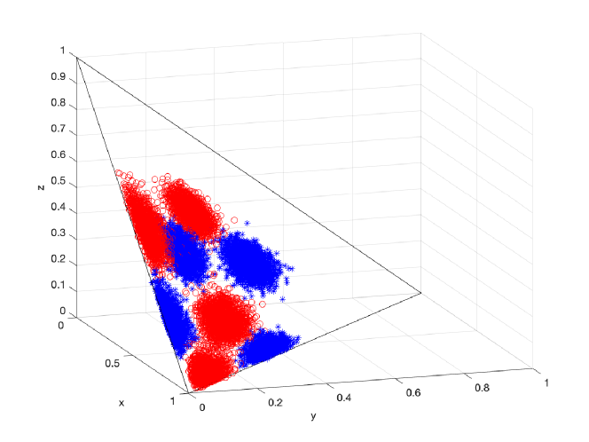
Figure 1: Compositional data illustration.

2.3 Hierarchical mixture of DGD classifiers

As described in [togban2018classification], when we face a difficult classification task, we can hierarchically combine several classifiers to form a meta-classifier. Firstly, at each level of the hierarchy, a set of parametric gating functions split the input space into several regions or modes. Finally, each classifier discriminates the data belonging to a specific region. Intuitively, the gating functions perform a classification task with an unknown label which refers to a region. Since the gating functions and the classifiers perform a classification task on the compositional data, we can model them with the classifier defined in equation (5). We call this hierarchy of DGD models, Hierarchical mixture of DGD experts (HMGD). This model can be viewed as a tree where each node (root, inner nodes and leaves) is linked to a DGD model. The root is related to the first division of the data into regions. The inner nodes are related to the division of the regions (resp. sub-regions) into sub-regions and the leaves embed the base classifiers (see Fig. 2). The base classifiers will be called experts as in HME literature [Jordan1993]. For a tree of two levels, we have the following formulation for HMGD:

$$\begin{array}[]{r}p\left(y|x,\,\Omega\right)=\overset{K}{\underset{i=1}{\sum}}\pi_{i}^{(0)}\left(x\right)\overset{M_{i}}{\underset{j=1}{\sum}}\pi_{j|i}^{(1)}\left(x\right)p\left(\mathbf{y}|x,\,\Omega_{ij}^{(2)}\right)\mid\,\pi_{i}^{(0)}\left(x\right)\geq 0;\;\pi_{j|i}^{(1)}\left(x\right)\geq 0\\ s.t.\,\overset{K}{\underset{i=1}{\sum}}\;\pi_{i}^{(0)}\left(x\right)=1;\;\overset{M_{i}}{\underset{j=1}{\sum}}\pi_{j|i}^{(1)}\left(x\right)=1.\par\end{array}$$ (6)

where $\pi_{i}^{(0)}\left(x\right)$ and $\pi_{j|i}^{(1)}\left(x\right)$ are respectively the gating functions of the first and second levels. The number of regions and sub-regions are respectively denoted by $K$ and $M_{i}$. For a tree with $L$ levels, we denote $\Omega=\{\Omega^{(l)}\}^{L}_{l=0}$ the set of all parameters where $\Omega^{(l)}=\{\alpha^{(l)},\mu^{(l)}\}^{L}_{l=0}$ is the set of parameters at the $l^{th}$ level. The gating functions parameters are $\Omega^{(0)}$ and $\{\Omega^{(l)}\}^{L-1}_{l=1}$ and the experts parameters are $\Omega^{(L)}$. The model HMGD is an extension of the model DME that we proposed in an earlier work [Togban2017]. There is no hierarchy in DME and the gating functions are based on the Dirichlet distribution. Moreover, the experts used are multinomial logistic regression.

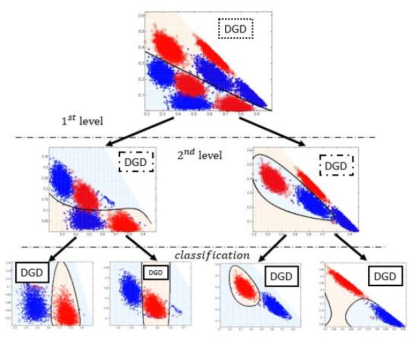
(a) Splitting process.

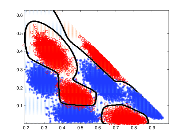
(b) Final decision boundary.

Figure 2: Illustration of the HMGD splitting process and the final decision boundary. The solid curve is the regions (resp. sub-regions or classes) boundary. In ”a)” each split is performed by a DGD model.

3 Parameters Estimation using Maximum Likelihood (ML)

Let $\mathbf{Obs}=\left\{\mathbf{X},\,\mathbf{Y}\right\}$ be a set of observed data where $\mathbf{X}=\{x_{1},\cdots,x_{N}\}\in\mathbb{R}^{D\times N}$ is a set of i.i.d. vectors and $\mathbf{Y}=\left(y_{1},\cdots,y_{N}\right)^{T}\in\mathbb{R}^{N}$ their equivalent class labels; $N$ is the number of observations. Since our model (eq. 6) is a mixture model, we can use EM algorithm for the training process. As in [togban2018classification], we introduce a set of ‘hidden’ binary random variables for the $n^{th}$ data: $z_{n,i}^{(0)}$ and $z_{n,j|i}^{(1)}$ respectively for the top-level and the lower-level of the tree. If $x_{n}$ belongs to the region $i$ then $z_{n,i}^{(0)}=1$ and 0, otherwise. Given the region $i$, if $x_{n}$ belongs to the sub-region $j$ then $z_{n,j|i}^{(1)}=1$ and 0, otherwise. The complete-log-likelihood can be written as follows:

$$\begin{array}[]{rr}\mathcal{L}^{c}=&\overset{N}{\underset{n=1}{\sum}}\overset{K}{\underset{i=1}{\sum}}z_{n,i}^{(0)}\overset{M_{i}}{\underset{j=1}{\sum}}z_{n,j|i}^{(1)}\ln\left(\pi_{i}^{(0)}\left(x_{n}\right)\pi_{j|i}^{(1)}\left(x_{n}\right)p\left(y_{n}|x_{n},\,\Omega_{ij}^{(2)}\right)\right)\end{array}$$ (7)

In the E-step we compute the following expectation:

$$\begin{array}[]{r}\Phi\left(\Omega,\,\Omega^{t}\right)=\overset{N}{\underset{n=1}{\sum}}\overset{K}{\underset{i=1}{\sum}}h_{n,i}^{(0)}\overset{M_{i}}{\underset{j=1}{\sum}}h_{n,j|i}^{(1)}\ln\left(\pi_{i}^{(0)}\left(x_{n}\right)\pi_{j|i}^{(1)}\left(x_{n}\right)p\left(y_{n}|x_{n},\,\Omega_{ij}^{(2)}\right)\right)\end{array}$$ (8)

where $\Omega^{t}$ is the parameters at the $t^{th}$ iteration; $h_{n,i}^{(1)}$ and $h_{n,j|i}^{(2)}$ are respectively the expected values of $z_{n,i}^{(0)}$ and $z_{n,j|i}^{(1)}$ and their expressions are given by

$$\begin{array}[]{ll}h_{n,i}^{(0)}=&\mbox{\Large$\frac{\pi_{i}^{(0)}\left(x_{n}\right)\overset{M_{i}}{\underset{j=1}{\sum}}\pi_{j|i}^{(1)}\left(x_{n}\right)p\left(y_{n}|x_{n},\,\Omega_{ij}^{(2)}\right)}{\overset{K}{\underset{i=1}{\sum}}\pi_{i}^{(0)}\left(x_{n}\right)\overset{M_{i}}{\underset{j=1}{\sum}}\pi_{j|i}^{(1)}\left(x_{n}\right)p\left(y_{n}|x_{n},\,\Omega_{ij}^{(2)}\right)}$}\end{array}$$ (9)

and

$$\begin{array}[]{ll}h_{n,j|i}^{(1)}=&\mbox{\Large$\frac{\pi_{j|i}^{(1)}\left(x_{n}\right)p\left(y_{n}|x_{n},\,\Omega_{ij}^{(2)}\right)}{\overset{M_{i}}{\underset{j=1}{\sum}}\pi_{j|i}^{(1)}\left(x_{n}\right)p\left(y_{n}|x_{n},\,\Omega_{ij}^{(2)}\right)}$}\end{array}$$ (10)

In the M-Step, we have to perform the following maximization operations:

$$\begin{array}[]{r}\Omega_{(t+1)}^{(0)}=argmax_{\Omega^{{}^{(0)}}}\overset{N}{\underset{n=1}{\sum}}\overset{K}{\underset{i=1}{\sum}}h_{n,i}^{(0)}\ln\left(\pi_{i}^{(0)}\left(x_{n}\right)\right)\end{array}$$ (11)

$$\begin{array}[]{lr}\Omega_{i,(t+1)}^{(1)}=&argmax_{\Omega_{i}^{{}^{(1)}}}\overset{N}{\underset{n=1}{\sum}}h_{n,i}^{(0)}\overset{M_{i}}{\underset{j=1}{\sum}}h_{n,j|i}^{(1)}\ln\left(\pi_{j|i}^{(1)}\left(x_{n}\right)\right)\end{array}$$ (12)

$$\begin{array}[]{r}\Omega_{ij,(t+1)}^{(2)}=argmax_{\Omega_{ij}^{{}^{(2)}}}\overset{N}{\underset{n=1}{\sum}}h_{n,i}^{(0)}h_{n,j|i}^{(1)}\overset{C}{\underset{c=1}{\sum}}v_{n,c}\ln\left(p\left(y_{n}=c|x_{n},\,\Omega_{ij}^{(2)}\right)\right)\end{array}$$ (13)

where $\Omega_{(t+1)}^{(l)}$ is the parameters $\Omega^{(l)}$ at the $(t+1)^{th}$ iteration and $v_{n,c}$ are binary variables indicating membership of $n^{th}$ data to the $c^{th}$ class. In general, for each node (at the $l^{th}$ level) being the $i^{th}$ child of its parent, we have to solve a weighted-DGD:

$$\begin{array}[]{l}\Omega_{i,(t+1)}^{(l)}=argmax_{\Omega_{i}^{{}^{(l)}}}\Phi^{(l)}\mid\Phi^{(l)}=\overset{N}{\underset{n=1}{\sum}}H_{n,i}^{(l-1)}\overset{M_{i}}{\underset{j=1}{\sum}}h_{n,j|i}^{(l)}\ln\left(\pi_{j|i}^{(l)}\left(x_{n}\right)\right)\end{array}$$ (14)

where $h_{n,j|i}^{(l)}$ acts like a label, $H_{n,i}^{(l-1)}$ is the product of all responsibilities along the path going from the root to the current node and act like a weight. When we are in the presence of a leaf, $h_{n,j|i}^{(L)}\equiv v_{n,c}$ and $M_{i}\equiv C$. As shown in figure (2a), the plot at the first level is obtained by performing a DGD model with a ”virtual label” while at the second level, we perform a weighted-DGD with a ”virtual label”. At the classification step, we perform a weighted-DGD with the true label.

3.1 Upper-bound for the GD mixture model

Given the expression of DGD model (eq. 5), the maximization operations in the M-Step lead to highly nonlinear optimization problems. The term leading to an optimization challenge is the mixture appearing in the denominator of equation (5). Previous works [xu1995alternative, Togban2017, togban2018classification] deal with this problem by performing the EM algorithm on the joint probability $p(\mathbf{y},\mathbf{x}|\,\Omega)$. Unfortunately, this solution is not suitable for a hierarchical case since it simplifies the problem just for the first level parameter. However, it is possible to circumvent this problem by using a variational approximation. Therefore, we have to optimize a lower-bound of the objective function $\Phi^{(l)}$ described in equation 14. This is equivalent to determine a lower-bound for the term $\ln\left(\dfrac{\alpha_{ij}^{(l)}GD(x|\mu_{ij}^{(l)})}{\underset{k=1}{\sum}\alpha_{ik}^{(l)}GD(x|\mu_{ik}^{(l)})}\right)$. Specifically, we need to find an upper-bound for $\ln\left(\underset{k}{\sum}\alpha_{ik}^{(l)}GD(x|\mu_{ik}^{(l)})\right)$. Exploiting the reverse Jensen inequality for a mixture of exponential family proposed in [jebara2001discriminative], we derived the following bound:

$$\begin{array}[]{l}\ln\left(\underset{k}{\sum}\alpha_{ik}^{(l)}GD(x_{n}|\mu_{ik}^{(l)})\right)\leq\underset{k}{\sum}-W_{n,ik}^{(l)}\left[\ddot{\mathbf{x}}_{n,ik}^{(l)T}\bar{\Omega}_{ik}^{(l)}-\mathcal{K}(\bar{\Omega}_{ik}^{(l)})\right]+cst_{n,i}\end{array}$$ (15)

Where

$$cst_{n,i}=\ln\left(\underset{k}{\sum}\breve{\alpha}_{ik}^{(l)}GD(x_{n}|\breve{\mu}_{ik}^{(l)})\right)+\underset{k}{\sum}W_{n,ik}^{(l)}\left[\ddot{\mathbf{x}}_{n,ik}^{(l)T}\breve{\Omega}_{ik}^{(l)}-\mathcal{K}(\breve{\Omega}_{ik}^{(l)})\right]$$

$$\ddot{\mathbf{x}}_{n,ik}^{(l)}=\dfrac{\tilde{\pi}_{k|i}^{(l)}\left(x_{n}\right)}{W_{n,ik}^{(l)}}\left[\mathcal{K}^{\prime}(\breve{\Omega}_{ik}^{(l)})-\bar{\mathbf{x}}_{n,ik}^{(l)}\right]+\mathcal{K}^{\prime}(\breve{\Omega}_{ik}^{(l)})$$ (16)

$$W_{n,ik}^{(l)}=4G\left(\breve{\pi}_{k|i}^{(l)}\left(x_{n}\right)/2\right)\left[\mathcal{Z}_{n,ik}^{(l)t}\mathcal{Z}_{n,ik}^{(l)}\right]+w_{n,ik}^{(l)}$$

$$\mathcal{Z}_{n,ik}^{(l)}=\mathcal{K}^{\prime\prime}(\breve{\Omega}_{ik}^{(l)})^{-1/2}\left[\bar{\mathbf{x}}_{n,ik}^{(l)}-\mathcal{K}^{\prime}(\breve{\Omega}_{ik}^{(l)})\right].$$

More details about the expressions involved in this upper-bound are given in appendix LABEL:appendix_upper. The parameter $\bar{\Omega}_{ik}^{(l)}$ is a re-parameterization of $\Omega_{ik}^{(l)}$ and $\breve{\pi}_{k|i}^{(l)}\left(x_{n}\right)$ is computed at the tangential contact point $\breve{\Omega}_{ik}^{(l)}$ (previous value of $\Omega_{ik}^{(l)}$). The expressions $\ddot{\mathbf{x}}_{n,ik}^{(l)}$ and $W_{n,ik}^{(l)}$ are variational parameters. The scalar $w_{n,ik}^{(l)}$ is the minimum value of $W_{n,ik}^{(l)}$ which guarantee that $\ddot{\mathbf{x}}_{n,ik}^{(l)}$ belong to the tangent space of $\mathcal{K}(\Omega_{ik}^{(l)})$. The expressions $\mathcal{K}^{\prime}(\Omega_{ik}^{(l)})$ and $\mathcal{K}^{\prime\prime}(\Omega_{ik}^{(l)})$ are respectively the gradient and the Hessian of $\mathcal{K}(\Omega_{ik}^{(l)})$ and $G$ is a linear function defined by a lookup table [jebara2001discriminative]. In order to visualize this upper bound, we plot both the log-likelihood of a mixture of beta distribution (Fig. 3a) and its equivalent upper-bound (Fig. 3b). The mixture used is: $0.3\;\mathtt{Beta}(x|a_{1},50)+0.7\;\mathtt{Beta}(x|a_{2},100)$. The log-likelihood is plotted with respect to $a_{1}$ and $a_{2}$. The tangential contact point (red circle) is fixed at $a_{1}=20$ and $a_{2}=50$. Let us recall that the Beta distribution is a particular case of the GD distribution.

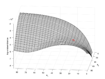
(a) Log-Likelihood to bound.

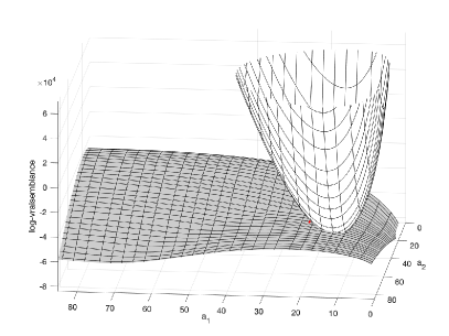
(b) Upper Bound of the Log-Likelihood.

Figure 3: Log-Likelihood of two Beta mixture and its upper-bound generated at the red circle point.

Given the upper-bound of GD mixture (eq. 15), we can derive the following lower-bound :

$$\begin{array}[]{r}\ln\left(\dfrac{\alpha_{ij}^{(l)}GD(x|\mu_{ij}^{(l)})}{\underset{k=1}{\sum}\alpha_{ik}^{(l)}GD(x|\mu_{ik}^{(l)})}\right)\geq\ln\left(\alpha_{ij}^{(l)}GD(x|\mu_{ij}^{(l)})\right)+cst_{n,i}\\ +\underset{k}{\sum}W_{n,ik}^{(l)}\left[\ddot{\mathbf{x}}_{n,ik}^{(l)T}\bar{\Omega}_{ik}^{(l)}-\mathcal{K}(\bar{\Omega}_{ik}^{(l)})\right]\par\end{array}$$ (17)

3.2 Parameters Estimation for DGD and HMGD models

Given the objective function $\Phi^{(l)}$ (Eq. 14) and the bound described in equation 17, we can perform the maximization operations on the following lower-bound:

$$\begin{array}[]{c}\Phi_{1}^{(l)}=\underset{n,j}{\sum}H_{n,i}^{(l-1)}\left[h_{n,j|i}^{(l)}\ln\left(\alpha_{ij}^{(l)}GD(x_{n}|\mu_{ij}^{(l)})\right)\right.\\ \left.+W_{n,ij}^{(l)}\left[\ddot{\mathbf{x}}_{n,ij}^{(l)t}\bar{\Omega}_{ij}^{(l)}-\mathcal{K}(\bar{\Omega}_{ij}^{(l)})\right]+cst_{n,i}\right]\\ \Phi_{1}^{(l)}\leq\Phi^{(l)}\end{array}$$ (18)

Thanks to the transformation of equation 4, the parameters $\mu_{ij,d}^{(l)}$ can be estimated independently for each $d\in\left\{1\cdots D\right\}$ via the Newton-Raphson method. Since $\mu_{ij,d}^{(l)}$ has to be strictly positive, we re-parametrize by setting $\mu_{ij,d}^{(l)}=e^{\xi_{ij,d}^{(l)}}$ where $\mu_{ij,d}^{(l)}$ is a vector with $a_{ij,d}^{(l)}$ and $b_{ij,d}^{(l)}$ as elements. The partial derivative of $\Phi_{1}^{(l)}$ (Eq. 18) with respect to $\xi_{ij,d}^{(l)}$ is given by:

$$\begin{array}[]{c}\dfrac{\partial\;\Phi_{1}^{(l)}}{\partial\xi_{ij,d}^{(l)}}=\mu_{ij,d}^{(l)}[\mathsf{\Psi}(|\mu_{ij,d}^{(l)}|)-\mathsf{\Psi}(\mu_{ij,d}^{(l)})-\ln(A)]\underset{n}{\sum}H_{n,i}^{(l-1)}\left[h_{n,j|i}^{(l)}+W_{n,ij}^{(l)}\right]+\\ \mu_{ij,d}^{(l)}\underset{n}{\sum}H_{n,i}^{(l-1)}\left[h_{n,j|i}^{(l)}\tilde{\mathtt{v}}_{n,d}+W_{n,ij}^{(l)}\chi_{n,ij}^{(l)}\right]\end{array}$$ (19)

where $\mathsf{\Psi}$ is the Digamma function, $\tilde{\mathtt{v}}_{n,d}=(\ln(\mathtt{v}_{n,d}),\;\ln(A-\mathtt{v}_{n,d}))^{T}$ and $\displaystyle\chi_{n,ij}^{(l)}=(\ddot{\mathbf{x}}_{n,ij,2d-1}^{(l)},\ddot{\mathbf{x}}_{n,ij,2d}^{(l)})^{T}$. The Hessian $\mathcal{H}_{ij,d}^{(l)}$ is a $2\times 2$ symmetric matrix where the diagonal elements are given by:

$$\begin{array}[]{r}[\mu_{ij,d}^{(l)}]^{2}\big{[}\mathsf{\Psi}^{\prime}(|\mu_{ij,d}^{(l)}|)-\mathsf{\Psi}^{\prime}(\mu_{ij,d}^{(l)})\big{]}\underset{n}{\sum}H_{n,i}^{(l-1)}\left[h_{n,j|i}^{(l)}+W_{n,ij}^{(l)}\right]+\dfrac{\partial\;\Phi_{1}^{(l)}}{\partial\xi_{ij,d}^{(l)}}\end{array}$$

and the anti-diagonal elements are given by

$$\begin{array}[]{l}a_{ij,d}^{(l)}b_{ij,d}^{(l)}\mathsf{\Psi}^{\prime}(|\mu_{ij,d}^{(l)}|)\underset{n=1}{\sum}\left[h_{n,j|i}^{(l)}+W_{n,ij}^{(l)}\right]\end{array}$$

where $\mathsf{\Psi}^{\prime}$ is the Trigamma function and $|.|$ is the $l1-norm$. Giving an initial $[\xi_{ij,d}^{(l)}]^{old}$, we have the following update equation:

$$[\xi_{ij,d}^{(l)}]^{new}=[\xi_{id}^{(l)}]^{old}-[\mathcal{H}_{ij,d}^{(l)}]^{-1}\dfrac{\partial\;\Phi_{1}^{(l)}}{\partial\xi_{ij,d}^{(l)}}$$ (20)

We give more details in appendix LABEL:appendix_inv to compute the inverse of the Hessian $\mathcal{H}_{ij,d}^{(l)}$ in an efficient way. Deriving $\Phi_{1}^{(l)}$ (Eq. 18) with respect to $\alpha_{ij}^{(l)}$ and taking into account the constraint ${\underset{j}{\sum}}\alpha_{ij}^{(l)}=1$, we have the following update equation,
for $j=1\cdots M_{i}-1$:

$$\begin{array}[]{l}[\alpha_{ij}^{(l)}]^{new}=\mbox{\Large$\frac{\underset{n}{\sum}H_{n,i}^{(l-1)}h_{n,j|i}^{(l)}+\underset{n,k}{\sum}H_{n,i}^{(l-1)}W_{n,ik}^{(l)}\ddot{\mathbf{x}}_{n,ik,2D+j}^{(l)}}{\underset{n}{\sum}H_{n,i}^{(l-1)}+\underset{n,k}{\sum}H_{n,i}^{(l-1)}W_{n,ik}^{(l)}}$}\\ [\alpha_{iM_{i}}^{(l)}]^{new}=1-\overset{M_{i}-1}{\underset{j=1}{\sum}}[\alpha_{ij}^{(l)}]^{new}\end{array}$$ (21)

Table 1 summarize the main parameters used in our model at the $l^{th}$ level of the tree.To choose the structure of the HMGD tree, we can set a large value for $K$ and $M_{i}$ and remove the components that have a weak value of $\alpha_{ij}^{(l)}$ after each iteration or after the algorithm had converged.

Table 1: The main parameters used in our model at the $l^{th}$ level of the tree given the parent node $i$ and the child $j$.

Symbol	Meaning
$\alpha_{ij}^{(l)}$	Mixing coefficients
$\mu_{ij}^{(l)}=\left\{a_{ij}^{(l)},b_{ij}^{(l)}\right\}$	Parameters of the GD distribution
$\Omega_{ij}^{(l)}=\left\{\mu_{ij}^{(l)},\alpha_{ij}^{(l)}\right\}$	the parameters of $\pi_{j|i}^{(l)}$
$\mathcal{K}(.)$	Cumulant function of GD distribution
$W_{n,ij}^{(l)},\ddot{\mathbf{x}}_{n,ij}^{(l)}$	Variational parameters for the mixture of GD’s upper-bound
$\ddot{\mathbf{x}}_{n,ij,d}^{(l)}$	$d^{th}$ element of $\ddot{\mathbf{x}}_{n,ij}^{(l)}$

The learning procedure for the DGD model is summarized in algorithm 1.

1. Initialization:

(a) For each class $c$, initialize $\mu_{c}$ through the moment method [minka2000estimating].

(b) set $\left\{\alpha_{c}\right\}_{c=1}^{C}$ as the prior of each class ($\alpha_{c}=N_{c}/N$) where $N_{c}$ is the number of instance belonging to the $c^{th}$ class.

2. E-step: Compute the variational parameters via equation 16 and the log-likelihood via equation (14) by replacing $h_{n,j|i}^{(l)}$ with the true label. Here, the weight $H_{n,i}^{(l-1)}$ is removed.

3. M-step: Maximize $\Phi^{(0)}$ (eq. 14) with respect to the current value of $\Omega^{(0)}$ and update $\Omega^{(0)}$ via equations (19 21).

4. Repeat steps 2 and 3 until convergence.

Algorithm 1 Learning algorithm for the DGD model

Since The HMGD is a combination of several (weighted) DGD, we can use the learning procedure summarized in algorithm 2.

1. Initialization:

(a) set the parameters $\left\{\Omega^{(l)}\right\}_{l=0}^{L-1}$ by using the procedures described in [bouguila2004unsupervised].

(b) set $\Omega^{(L)}$ like in algorithm (1) for the instances belonging to each subregions.

2. E-step: Update $Q\left(\Omega,\,\Omega^{t}\right)$ via equations (8 10) and compute the variational parameters via equation 16.

3. M-step: the new parameters given the old ones as initialization are obtained for:

(a) $\{\pi_{i}^{(0)}\}^{K}_{i=1}$ by running the DGD algorithm with $\{h_{n,i}^{(0)}\}^{K}_{i=1}$ as labels.

(b) $\{\pi_{j|i}^{(l)}\}^{(L-1),M_{i}}_{l,j=1}$ by running a weighted DGD algorithm with $h_{n,j|i}^{(l)}$ as label and $H_{n,i}^{(l-1)}$ as weight for a given $i$ and $l$.

(b) each classifier by running a weighted DGD algorithm with the true label and $H_{n,i}^{(L-1)}$ as weight.

4. Repeat steps 2 and 3 until convergence.

Algorithm 2 Learning algorithm for the HMGD model

4 Experimental Results and discussion

To assess the performance of our models, we have firstly conducted our experiment on several datasets from UCI machine learning repository [Lichman2013]. Secondly, we have considered some real-world applications namely spam detection and color space identification. In all the experiments, we set the EM convergence tolerance to $10^{-4}$ over 50 maximum iterations for the DGD model. In the case of HMGD, to reduce the overfitting, we set the maximum number of iterations to 10. For the gating functions and the experts, the maximum number of iterations is respectively set to 5 and 30. In general, we observed that a number of iterations greater than those indicated earlier led to overfitting. Since the GD is not defined for zero values, we replace them with a small value ($1e-4$) [martin2003dealing].

All the results are based on a five stratified cross-validation (5-CV). This choice is justified by the fact that stratified cross-validation helps to improve the generalization ability of a classifier. We used the accuracy and the Matthew’s correlation coefficient (MCC) as evaluation criteria for all the models. In the case of imbalanced data, MCC is a better choice than accuracy, precision, recall and F1-score regardless which class is positive [mcc_article, chicco2020advantages]. This coefficient vary from $-1$ to $1$. When the values are negatives, the classifier perform poorly and when they are close to zero we have a random guess classifier. The best classifiers have an MCC value close to $1$.

4.1 Evaluation of DGD and HMGD on UCI datasets

In this section, we conducted our study on six datasets from UCI machine learning repository [Lichman2013]. The goal of this study is to compare the models DGD, HMGD, HMD1 [togban2018classification], DME [Togban2017], Multinomial logistic regression (MLR) as well as the mixture of Generalized Dirichlet (MGD). The model HMD1 is a two levels hierarchical mixture model where the experts are multinomial logistic regressions. In HMD1, the first level gating function is based on Gaussian distribution and the second level gating function is chosen as a Softmax function. For the MGD model, each class is described by a Generalized Dirichlet and the class membership is given by the a posteriori probability. Estimate the parameters of MGD is equivalent to estimate the parameters of DGD by setting the variational parameters to zero. The comparison between MGD and DGD will help us to evaluate the relevance of the upper-bound described above. Let us recall that HMD1 and DME combine several logistic regressions through different type of gating functions. In order to obtain compositional data we:1) delete the binary features, 2) standardize the data (mean is equal to zero and standard equal to one), 3) rescale the data between zero and one and normalize them to get data lying in the simplex. Table (2) present the main characteristics of the datasets used.

Table 2: UCI Datasets used to evaluate the models DGD and HMGD.

2pt Datasets #instances dimension #classes Appendicitis 106 7 2 Vowel 990 10 11 Cancer (Breast) 277 9 2 Magic 19,020 10 2 Vehicle 946 18 4 Satimage 6 435 4 6

The accuracies are reported in table (3) and the number in brackets refer to the number of experts used in HMGD, HMD1, HMD2, DME. To choose the number of experts, we used the method described in [togban2018classification]. We plot the MCC values in figure4.

Table 3: Comparison of DGD, MGD, HMGD, DME, HMD1 and LR.

0pt 2pt Magic (5) Veh.(4) Vow. (4) Appe. (2) Sat. (4) Cancer (2)     Mean MLR 78.5 $\pm$ 0.39 40.8 $\pm$ 12.44 64.04 $\pm$ 3.34 84.89 $\pm$ 4.03 74.33 $\pm$ 0.58 72.94 $\pm$ 8.43     69.25 MGD 77.25 $\pm$ 1.43 52.96 $\pm$ 5.6 66.36 $\pm$ 4.47 83.07 $\pm$ 5.11 77.53 $\pm$ 0.69 71.49 $\pm$ 4.6     71.44 HMD1 83.65 $\pm$ 0.74 44.09 $\pm$ 6.56 86.16 $\pm$ 4.53 86.80 $\pm$ 2.08 75.34 $\pm$ 0.62 72.57 $\pm$ 6.93     74.76 DME [Togban2017] 83.84 $\pm$ 0.53 55.09 $\pm$ 6.5 84.04 $\pm$ 3.81 84.98 $\pm$ 8.26 75.31 $\pm$ 0.74 70.4 $\pm$ 7.09     75.61 DGD 82.23 $\pm$ 0.8 62.17 $\pm$ 7.12 79.49 $\pm$ 3.08 86.8 $\pm$ 3.96 78.15 $\pm$ 0.61 72.22 $\pm$ 4.6     76.52 HMGD 83.22 $\pm$ 0.83 68.91 $\pm$ 8.37 88.79 $\pm$ 0.9 87.75 $\pm$ 2.5 78.91 $\pm$ 0.52 72.22 $\pm$ 3.09     79.97

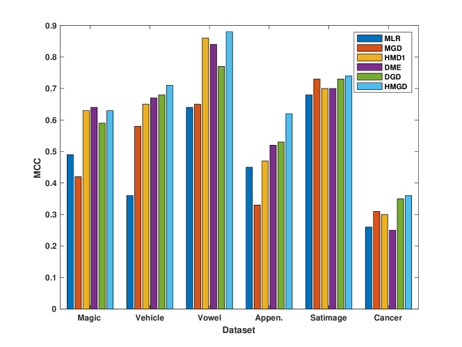
Figure 4: Matthew Correlation Coefficient according to the results of table 3.

The results vary from one dataset to another. On Magic dataset, DGD and HMGD improve by at least 4% the accuracy obtained by multinomial logistic regression and MGD. However, the standard deviations obtained by DGD and HMGD are slightly higher than the one obtained by multinomial logistic regression. On this dataset, HMD1 and DME slightly outperform HMGD (the variation of accruracy is below 1%). With Vehicle dataset, DGD achieves an accuracy at least 7% more than MGD, HMD1 and DME. However, the standard deviation of DGD is slighter higher than the ones obtained these four models (variation is below 1%). The model DGD obtained a better accuracy compared to MGD on all the six datasets used in our experiment. In the case where the standard deviation obtained by MGD is lower than the one obtained by DGD (almost 2% of variation), the accuracy of DGD is 9% higher. The model DGD achieves a better accuracy compared to HMD1 on the datasets Vehicle and Satellite. With these two datasets, the standard deviation obtained by DGD and HMD1 are similar. The model HMGD achieves a better accuracy compared to HMD1 ( between 1% and 6% higher) on datasets Vowel, Appendicitis and Satimage. Moreover, on these three datasets, the standard deviation obtained by HMGD is lower than the one obtainded by HMD1. With the Cancer dataset, compared to HMD1, HMGD obtained a better standard deviation (3% lower) while both achieve a similar accuracy. In general, HMGD improve the accuracy and the standard deviation obtained by DGD. In the cases where the standard deviation obtained by HMGD is higher than the one obtained by DGD, the variation is small compared to the gain in accuracy. For all datasets, the MCC values confirm with the scores obtained with the accuracy measure.

4.2 Spam Detection

Spams are irrelevant messages send to a set of recipients. These messages can contain malicious software or phishing programs. According to Kaspersky [Kap2020], 56.51 % of the emails received in 2019 were spams. It is important to detect those spams in order to avoid boring the recipients, allowing them to focus on essential emails or protecting them from criminal activities. For this purpose, several supervised methods have been used [jain2019optimizing, Ankam2018, dada2019machine]. We use our models DGD and HMGD to deal with spam detection problem. We compare our models against HMD1 [togban2018classification], MLR and MGD. The goal here is to compare the strategy of applying the alpha-transformation (eq. 1) to the data with our models. Therefore, for the models HMD1 and MLR, we preprocessed the data with the $\alpha$-transformation (1). In our experiments, we vary $\alpha$ from 0 to 1 with 0.2 as step. The accuracy is reported in table (4). The number in parentheses represents the number of experts used. The number following the symbol $\pm$ is the standard deviation. We performed our experiments on two datasets previously used in the literature of spam detection [kumar2012comparative, Ankam2018].

i) HP Spambase has been created by Hewlett-Packard Labs and downloaded from UCI machine learning repository. This dataset has 4601 instances with 57 continuous attributes and the class label (spams or not). Spams represent 39.4% of the instances in this dataset. Since DGD and HMGD are designed for compositional data, we considered the 20 attributes representing the frequency of Words/Characters most used in this dataset. A spam detector can group the emails in three categories: legitimate, spams and needing more scrutiny. In order to create this third category, we randomly select 977 instances belonging to the legitimate category. Therefore, the new dataset has equal proportion of spams and legitimate messages (39.4% each) and 21.2% of messages needing more scrutiny. The accuracy obtained by MLR and HMD1 are similar to the one obtained by DGD. However, HMGD improve the results of DGD and outperform HMD1. Let us recall that in this study, HMD1 combines two multinomial logistic regressions while HMGD combines two DGD.

ii) Ling-spam is a dataset containing 2893 emails with 481 (16.6%) spams. We create a third category by selecting randomly 481 emails from the legitimate one. We obtain then a dataset composed of 1443 emails (481 emails per category). The features used are obtained by first, deleting stop words and by doing a lemmatization [Ankam2018]. After that, a word dictionary is created with the 30 most common words. The final feature is a vector containing the words frequency.

The models DGD and HMGD outperformed MLR, HMD1 and MGD in terms of accuracy (with lower standard deviation in the case of HMGD). We notice that HMGD improve both the accuracy and standard deviation obtained by DGD. The models DGD and HMGD achieve an accuracy of 2% to 3% higher than HMD1 and MLR using $\alpha$-transformation. As noted in the previous experiments, the variational approximation apply to the model DGD allow us to achieve better results compared to MGD. The MCC values obtained by DGD and HMGD suggest that the two models achieve a slightly better classification than MLR, MGD and HMGD.

Table 4: Comparison of DGD, HMGD, HMD1, MLR and MGD on the datasets HP Spambase and Ling-spam.

	MLR	MGD	HMD1 (2)	DGD	HMGD (2)
HP Spambase	73.51 $\pm$ 0.9 ($\mathbf{\alpha}^{*}=0$)	71.30 $\pm$ 0.83	73.49 $\pm$ 0.66 ($\mathbf{\alpha}^{*}=0$)	73.60 $\pm$ 0.85	74.47 $\pm$ 0.72
Ling-spam	62.81 $\pm$ 2.69 ($\mathbf{\alpha}^{*}=0.6$)	63.93 $\pm$ 2.92	62.67 $\pm$ 2.56 ($\mathbf{\alpha}^{*}=0.6$)	64.81 $\pm$ 3.01	66.07 $\pm$ 2.10

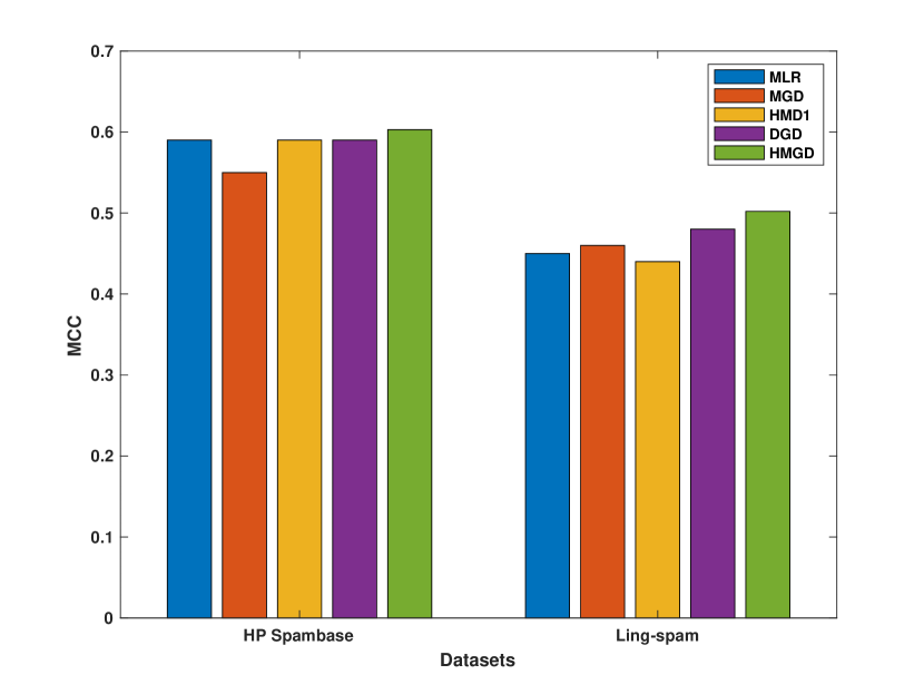
Figure 5: Matthew Correlation Coefficient according to the results of table 4.

4.3 color space identification

Color space is a color representation system based on a set of triplets. One of the most used color space for visualization is RGB, which is composed of the channels Red, Green and Blue. In order to faithfully represent color in different human activities (photography, displaying, industry), several variants of RGB have emerged such as sRGB, Adobe RGB, Apple RGB and ProPhoto RGB. It is important to correctly choose the color space of an image if we want to faithfully reproduce it. Some applications choose the color space by default for the purpose of displaying. For example, the color space use by default on the web is sRGB while image-editing software Adobe Lightroom use Adobe RGB. After editing an image, it is possible to embed in EXIF data, the information relative to the color space. Once this information is available, one can faithfully represent the image with any displaying devices. But for different reasons, the Exif data can be missing or damaged which will lead to a misrepresentation of the image.

The goal of our experiment is to discriminate between the color space in the RGB family. For this experiment, we have considered the color spaces sRGB, Apple RGB, ColorMatch RGB, Adobe RGB and ProPhoto RGB. The problem of color space identification was first addressed by Vezina et al. [martin2015]. In their work, they used gamut estimation to discriminate between sRGB, HSV, HLS and Lab color spaces. Unfortunately, in the case of the RGB family, we need a more accurate estimation of the gamut. However, it is possible to exploit the correlation between the pixels for color space identification. Let $I$ be a color image in a RGB color space. We assume that if there is a correlation between the pixels, their value can be expressed as follows:

$$\begin{array}{c}\hfill I(m,n,k)=\sum _{\begin{array}{c}(i,j)\in V(m,n)\end{array}}\gamma {}_{i,j,k}I(m+i,n+j,k)+w(m,n)\end{array}where\text{γ}\text{\_i,j,k}areasetofcoefficientswith\text{γ}\text{\_0,0,k=0},\text{k ∈{R,G,B}}refertothechannelsofRGB,\text{I(m,n,k)}isthevalueofthepixellocatedat\text{(m,n)}forthechannel\text{k}and\text{V(m, n)}itsneighborhood.Thevariable\text{w(m,n)}isaGaussianwhitenoisewithstandarddeviation\text{σ}.Basically,weassumethatifthepixelsarecorrelated,eachpixelvaluecanbeexpressedasalinearfunctionofitsadjacentpixels.Theparametersofthemodeldescribedinequation\text{<a href="\#Ax3.Ex16" title="4.3 color space identification ‣ 4 Experimental Results and discussion ‣ Hierarchical mixture of discriminative Generalized Dirichlet classifiers" class="ltx\_ref ltx\_font\_italic"><span class="ltx\_text ltx\_ref\_tag">4.3</span></a>}aregivenbythevector\text{γ}\text{\_k}with\text{{}\text{γ}\text{\_i,j,k∣(i,j) ∈V(m, n)}}aselementsand\text{σ}.Inthispaper,wedefinetheneighborhoodas\text{V(m,n)= {(i,j)∣-J≤i,j ≤J}}where\text{J}denotesthenumberofpixelslocatedoneithersideofthepixelatthelocation\text{(m,n)}.Inarecentwork\text{<cite class="ltx\_cite ltx\_citemacro\_cite">[<span class="ltx\_ref ltx\_missing\_citation ltx\_ref\_self">color\_2023</span>]</cite>},weshowthatthecorrelationcoefficients\text{γ}\text{\_i,j,k}canbeusedasfeaturestoidentifyRGBcolorspace.Thefeaturesdimensionis\text{3(2J+1)^2-3}.\text{Table 5Table 55Table 55Acc}$$