Geometry and purity properties of qudit Hamiltonian systems

J.A. López–Saldívar1,2,3, O. Castaños4,†, S. Cordero4, E. Nahmad–Achar4 and R. López–Peña4 1 Department of Theoretical Physics, Moscow Institute of Physics and Technology, Dolgoprudnyi 141700, Russia 2 Russian Quantum Center, Skolkovo, Moscow 143025, Russia 3 National University of Science and Technology “MISIS”, Moscow 119049, Russia 4 Instituto de Ciencias Nucleares, Universidad Nacional Autónoma de México, Apartado Postal 70-543, 04510 Mexico City, Mexico On sabbatical leave at University of Granada, Spain julio.lopez.8303@gmail.com ocasta@nucleares.unam.mx sergio.cordero@nucleares.unam.mx nahmad@nucleares.unam.mx lopez@nucleares.unam.mx , , , ,

Abstract

The principle of maximum entropy is used to study the geometric properties of an ensemble of finite dimensional Hamiltonian systems with known average energy. These geometric characterization is given in terms of the generalized diagonal Bloch vectors and the invariants of the special unitary group in n𝑛n dimensions. As examples, Hamiltonians written in terms of linear and quadratic generators of the angular momentum algebra are considered with J=1𝐽1J=1 and J=3/2𝐽32J=3/2. For these cases, paths as functions of the temperature are established in the corresponding simplex representations, as well as the adiabatic evolution of the interaction strengths of the Hamiltonian models. For the Lipkin-Meshkov-Glick Hamiltonian the quantum phase diagram is explicitly shown for different temperature values in parameter space.

Keywords: purity, thermal qudit states, geometric properties, maximum entropy, invariant spaces, LMG model

1 Introduction

Quantum information theory has become an important tool in the study of physical systems. Although the processing of quantum information is still a young field of research, it has yielded a deep change about the fundamental aspects of quantum mechanics. The main purpose of this field is the exploitation of the quantum features with a technological purpose [1, 2, 3, 4]. Differences between classical and quantum information are related to the possibility of having secure communications, to the solution of certain mathematical problems, and perhaps to having a quantum computer. All these benefits are due to properties of quantum mechanics such as uncertainty, interference, and entanglement. Thus, it becomes important to study the entanglement properties of quantum states, which implies the characterization of the entanglement, its application to quantum information processing and, from the mathematical point of view, the characterization and classification of positive maps on Csuperscript𝐶C^{*} algebras [2, 3, 4].

The first explicit relation made between physical entropy and information is associated to the relation between energy and information. This goes back to Maxwell’s demon paradox introduced in 1867, which implies an apparent violation of the second law of thermodynamics. The connection of information theory to physics helps to solve Maxwell’s demon paradox with the establishment of Landauer’s principle, that is, energy can be extracted from information [5, 6]. Shannon [7] establishes that if a message has n𝑛n symbols having transmission probabilities (p1,p2,,pn)subscript𝑝1subscript𝑝2subscript𝑝𝑛(p_{1},p_{2},\cdots,p_{n}) the amount of information in the message is,

S=i=1npilnpi.subscript𝑆subscriptsuperscript𝑛𝑖1subscript𝑝𝑖subscript𝑝𝑖\mathcal{H}_{S}=-\sum^{n}_{i=1}p_{i}\ln p_{i}\,. (1)

He called this quantity uncertainty, but von Neumann asked him to call it entropy arguing that a similar expression exists in statistical mechanics [6].

E. Jaynes in 1957 established that Shannon had actually uncovered a fundamental element of probability theory, that is, SSsubscript𝑆𝑆\mathcal{H}_{S}\equiv S defines the entropy of a probability distribution on an exhaustive set of mutually exclusive alternatives. The principle of maximum entropy PME establishes that the distribution {pk}subscript𝑝𝑘\{p_{k}\} that maximizes S𝑆S subject to the constraints imposed by the available information is the least biased description of what we know about the set of alternatives [8, 9, 10]. It has been proven that the PME is a correct method of inference when new information is given in terms of expectation values [11].

This rule provides a variational procedure for constructing prior probabilities on a given evidence. If we do not know something about a system, this rule establishes that the system has the same probability of staying in any of all its possible states, i.e., p=1/nsubscript𝑝1𝑛p_{\ell}=1/n and S=lnn𝑆𝑛S=\ln n. If the system is in one particular state k𝑘k, one has S=0𝑆0S=0. If the expectation value of the energy is known, the PME determines the Gibbs canonical ensemble, if the energy and number of moles are known one gets the Gibbs grand canonical ensemble, if the expectation values of the energy and angular momentum are known the PME determines the Gibbs rotational ensemble [12]. Additionally, the use of the PME for physical systems in thermal equilibrium can be extended to solve non-equilibrium problems because it can be applied to any physical quantity, be it density of particles, density of kinetic energy, components of the stress tensor, intensity of the magnetization, and so on.

Collective spin operators of multi-qudit systems generate a unitary algebra in n𝑛n dimensions, u(n)𝑛(n), and the concepts of pairwise entanglement and spin squeezing has been extended to describe general multi-qudit systems. The reduced density matrices of one and two qudits in the system of symmetric multi-qudits are used to determine, by means of the linear and von Neumann entropies, their entanglement properties. For the squeezing concept an embedding of the su(2)2(2) sub-algebras into u(n)𝑛(n) is proposed, which yields n𝑛n squeezing parameters. Both the entanglement and the squeezing parameters are good markers of the quantum phase transitions exhibited by the Lipkin-Meshkov-Glick Hamiltonian system of n𝑛n level interacting atoms and thus they can be used to establish the corresponding quantum information diagrams, and also through the inverse participation ratio concept to determine the corresponding localization properties in phase space [13, 14, 15].

There are several basis states for finite n𝑛n-dimensional systems: The generalized Gell-Mann vectors, those associated to the generators of the special unitary algebras SU(n𝑛n), the polarization operators, the Weyl operators, the Casimir invariants of SU(n𝑛n), and the canonical coset decomposition of unitary matrices [16, 17, 18, 19, 20]. In particular, we will consider in this work the generalized Bloch vectors because they allow us to determine the density matrix on the basis of actual measurements. The density matrix description of a state of n𝑛n-level systems requires n21superscript𝑛21n^{2}-1 real parameters and it can be written in the form [18, 20, 21]

𝝆=1n𝑰+12k=1n21λk𝚲k,𝝆1𝑛𝑰12superscriptsubscript𝑘1superscript𝑛21subscript𝜆𝑘subscript𝚲𝑘{\bm{\rho}}=\frac{1}{n}{{\bm{I}}}+\frac{1}{2}\sum_{k=1}^{n^{2}-1}\lambda_{k}\,{\bm{\Lambda}}_{k}\,, (2)

where 𝑰𝑰{{\bm{I}}} is the identity matrix in n𝑛n dimensions and λksubscript𝜆𝑘\lambda_{k} is the expectation value of the generator 𝚲ksubscript𝚲𝑘{\bm{\Lambda}}_{k}. The operator 𝝆𝝆{\bm{\rho}} is hermitian and satisfies Tr(𝝆)=1Tr𝝆1{\rm Tr}({\bm{\rho}})=1 because the generators 𝚲ksubscript𝚲𝑘{\bm{\Lambda}}_{k} of the special unitary algebra SU(n)𝑛(n) are complex traceless hermitian matrices. These generators have the property Tr(𝚲j𝚲k)=2δjkTrsubscript𝚲𝑗subscript𝚲𝑘2subscript𝛿𝑗𝑘{\rm Tr}({{\bm{\Lambda}}_{j}}{\bm{\Lambda}}_{k})=~{}2\,\delta_{j\,k}.

The important properties for the description of the density matrix state are the positivity condition 𝝆k0subscript𝝆𝑘0{\bm{\rho}}_{k}\geq 0 and the fact that 1/nTr(𝝆2)11𝑛Trsuperscript𝝆211/n\leq{\rm Tr}\,({\bm{\rho}}^{2})\leq 1, which are fundamental to determine the physical space of the density matrices [22, 23]. Notice that the generators are determined by means of the symmetric dijksubscript𝑑𝑖𝑗𝑘d_{ijk} and antisymmetric fijksubscript𝑓𝑖𝑗𝑘f_{ijk} structure constants of the mentioned special unitary algebra. The condition, Tr(𝝆2)1Trsuperscript𝝆21{\rm Tr}\,({\bm{\rho}}^{2})\leq~{}1 on (2) implies that the length of the Bloch vector is bounded, that is,

|λ|2(n1)n.𝜆2𝑛1𝑛|\lambda|\leq\sqrt{\frac{2\,(n-1)}{n}}\,. (3)

The density matrix (2) satisfies the positivity condition if its characteristic polynomial pρ(x)=det(x𝑰𝝆)subscript𝑝𝜌𝑥𝑥𝑰𝝆p_{\rho}(x)=\det(x{{\bm{I}}}-{\bm{\rho}}), viz.

pρ(x)=xna1xn1+a2xn2+(1)n1an1x+(1)nan,subscript𝑝𝜌𝑥superscript𝑥𝑛subscript𝑎1superscript𝑥𝑛1subscript𝑎2superscript𝑥𝑛2superscript1𝑛1subscript𝑎𝑛1𝑥superscript1𝑛subscript𝑎𝑛p_{\rho}(x)=x^{n}-a_{1}\,x^{n-1}+a_{2}\,x^{n-2}-\cdots+(-1)^{n-1}\,a_{n-1}\,x+(-1)^{n}\,a_{n}\,, (4)

has coefficients ak0subscript𝑎𝑘0a_{k}\geq 0 according to the Descartes theorem about the sign rules [24].

An additional remark is that the orbits generated by unitary transformations on the density matrices can be classified in terms of the Gram matrix, built from the Hilbert-Schmidt scalar products of the vectors lying in the tangent space of the orbits, and the rank of the Gram matrix determines the dimensions of the orbits. This classification is consistent with the results obtained by means of the stability groups of unitary transformations [25, 26]. Due to the invariance of the Gram matrix under unitary transformations, in order to determine the orbits one can consider the diagonal representation of the density matrix [27, 28, 29, 30].

An interesting feature of unitary group representations for quantum systems is their correspondence with different projective geometries as the Fano projective plane [31] with the 222-simplex of the qutrit system, or the projective space PG(3,2) [32] with the 333-simplex defined for a four-level system. See [33] and references therein for a study and historical perspective of the connection between quantum information processes to projective geometries and combinatorial design.

In this contribution, the physical space associated to the diagonal generalized Bloch vectors and the Casimir invariants is determined, in order to describe the well-defined density matrices of systems of qubits, qutrits, and ququarts. We use the PME to determine the density matrices of ensembles of qubits, qutrits, and ququarts with a defined average energy. These ensembles are described by Hamiltonians given in terms of linear and quadratic generators of the angular momentum algebra. By means of the diagonal decomposition of the density matrices associated to the linear and quadratic Hamiltonians, we may visualize geometrically the purity properties of ensembles with known average energy. In particular, the available paths in the corresponding simplex representations are established for the ensembles as a function of the temperature.

Section 2 gives a description of the Principle of Maximum Entropy for an ensemble of particles with a fixed averaged energy, which yields the Boltzmann probability density and at the same time minimizes the Helmholtz free energy of the quantum system. Different matrix representations of a density operator of an n𝑛n dimensional quantum system are also given, these being the probability, the Bloch-Gell-Mann, and the invariant cases. In addition, a general discussion of the thermal trajectories as a function of the temperature are given, from T0𝑇0T\to 0 (pure state) to T𝑇T\to\infty (the most mixed state). In section 3 the diagonal representations for the qutrit and ququart systems are established together with the corresponding mapping between them. Thus, one is able to exhibit the localization of the physical density matrices in the probability (p𝑝p)-, Gell-Mann (λ𝜆\lambda)-, and invariant (t𝑡t)-spaces, with and without eigenvalue degeneracy, the latter of which is associated to the higher dimensional orbits of the qutrit and ququart systems. In section 4, linear and quadratic Hamiltonian models in terms of the angular momentum operators are considered, particularly for J=1𝐽1J=1 (a realization in terms of identical but distinguishable dimers) and J=3/2𝐽32J=3/2 (a realization in terms of identical but distinguishable trimers). The behavior of the thermal states for the qutrit and ququart is obtained and visualized in the p𝑝p-, λ𝜆\lambda- and t𝑡t-spaces. For the Lipkin-Meshkov-Glick Hamiltonian model particular attention is paid to the quantum phase transitions and their influence on the characteristics of the corresponding thermal states in the diagonal representation. Section 5 gives a summary of the main results and additional remarks.

2 Variational thermal density matrix.

In quantum statistical mechanics the entropy is defined in terms of the density matrix

S=kBTr(𝝆ln𝝆),𝑆subscript𝑘𝐵Tr𝝆𝝆{S}=-k_{B}{\rm Tr}({{\bm{\rho}}\ln{{\bm{\rho}}}})\,, (5)

with the constraints Tr𝝆=1Tr𝝆1{\rm Tr}{{\bm{\rho}}}=1 and Tr𝝆21Trsuperscript𝝆21{\rm Tr}{{\bm{\rho}}^{2}}\leq 1. If one considers n𝑛n finite dimensional systems, the density operator has also another restriction Tr𝝆21/nTrsuperscript𝝆21𝑛{\rm Tr}{{\bm{\rho}}^{2}}\geq 1/n. According to the PME, the prior knowledge of an ensemble of quantum systems can be used to maximize the entropy. If the average energy Tr(𝝆𝑯)=E¯Tr𝝆𝑯¯𝐸{\rm Tr}({\bm{\rho}}\,{\bm{H}})=\bar{E} is known, one must then take the following variations: δS=0𝛿𝑆0\delta S=0, δ(Tr𝝆1)=0𝛿Tr𝝆10\delta({\rm Tr}{\bm{\rho}}-1)=0, and δ(Tr(𝝆H)E¯)=0𝛿Tr𝝆𝐻¯𝐸0\delta({\rm Tr}({\bm{\rho}}\,H)-\bar{E})=0, implying that [34]

Tr[(1+ln𝝆+ϵ+β𝑯)δ𝝆]=0,Trdelimited-[]1𝝆italic-ϵ𝛽𝑯𝛿𝝆0{\rm Tr}\left[(1+\ln{\bm{\rho}}+\epsilon+\beta\,{\bm{H}})\,\delta{\bm{\rho}}\,\right]=0\,, (6)

where we have introduced two Lagrange multipliers ϵitalic-ϵ\epsilon and β𝛽\beta. From the last expression one obtains the density matrix 𝝆𝝆{\bm{\rho}} and, taking its trace, ϵitalic-ϵ\epsilon is determined, yielding

𝝆=1Zexp(β𝑯),𝝆1𝑍𝛽𝑯{\bm{\rho}}=\frac{1}{Z}\exp{(-\beta\,{\bm{H}})}\,, (7)

with the partition function Z=Tr[exp(β𝑯)]𝑍Trdelimited-[]𝛽𝑯Z={\rm Tr}\left[\exp{(-\beta{\bm{H}})}\right]. In order to determine β𝛽\beta, one considers a cavity filled with photons in thermal equilibrium with the walls at temperature T𝑇T. In this case, and by means of the Correspondence Principle, one obtains β=1kBT𝛽1subscript𝑘𝐵𝑇\beta=\frac{1}{k_{B}\,T}. Notice that the maximization requirement of the entropy yields the expression

TSU+F=0,𝑇𝑆𝑈𝐹0T\,S-U+F=0\,, (8)

with the identification of the internal energy of the system U=𝑯𝑈delimited-⟨⟩𝑯U=\langle{\bm{H}}\rangle and the Helmholtz free energy F=kBTlnZ𝐹subscript𝑘𝐵𝑇𝑍F=-k_{B}T\ln Z. Therefore the PME implies also a minimum Helmholtz free energy of the system.

Expression (7) may be obtained by considering a closed system constituted by the Hamiltonian associated to one subsystem and the Hamiltonian of a heat bath, in which the interaction term can be ignored. In this case the composed system can also be represented by a micro-canonical ensemble in the energy interval E𝐸E and E+δE𝐸𝛿𝐸E+\delta E with δEEmuch-less-than𝛿𝐸𝐸\delta E\ll E. If the number of degrees of freedom of the bath is very large the reduced density matrix takes the form given in Eq. (2). This procedure has led to the answer of when is it possible to represent the reduced density matrix of the system 𝝆Ssubscript𝝆𝑆{\bm{\rho}}_{S} in terms of a wave function ψ𝜓\psi with 𝝆ψ=𝝆Ssubscript𝝆𝜓subscript𝝆𝑆{\bm{\rho}}_{\psi}={\bm{\rho}}_{S} [35, 36, 37].

Note, once again, that the variational method maximizes the von Neumann entropy and simultaneously minimizes the energy.

2.1 Matrix representations.

In order to study finite mixed quantum systems the use of the density matrix formalism is necessary. Besides (vide infra), to consider its diagonal form is convenient if one wishes to classify the different types of density matrices according to the dimension of the orbits in the tangent space.

The set of diagonal density matrices of dimension n𝑛n can be denoted in terms of their eigenvalues,

𝑫n=DiagM(p1,p2,pn1,pn),subscript𝑫𝑛DiagMsubscript𝑝1subscript𝑝2subscript𝑝𝑛1subscript𝑝𝑛{\bm{D}}_{n}={\rm DiagM}\,\left(p_{1},p_{2},\cdots p_{n-1},p_{n}\right)\,, (9)

with 0pk10subscript𝑝𝑘10\leq p_{k}\leq 1 and k=1npk=1subscriptsuperscript𝑛𝑘1subscript𝑝𝑘1\sum^{n}_{k=1}p_{k}=1. This set then forms a simplex in n1𝑛1n-1 dimensions (cf. e.g. [38]). A general density matrix can be constructed from them via

𝝆=𝑼𝑫n𝑼,𝝆𝑼subscript𝑫𝑛superscript𝑼{\bm{\rho}}={\bm{U}}\,{\bm{D}}_{n}{\bm{U}}^{\dagger}\,, (10)

where 𝑼𝑼{\bm{U}} denotes a unitary transformation in n𝑛n dimensions, U(n)𝑛(n). The set of transformations leaving 𝑫nsubscript𝑫𝑛{\bm{D}}_{n} invariant form a group called the stability group {\cal H}, i.e.,

𝑻𝑫n𝑻=𝑫n𝝆=𝛀𝑫n𝛀,formulae-sequencesubscript𝑻subscript𝑫𝑛superscriptsubscript𝑻subscript𝑫𝑛𝝆𝛀subscript𝑫𝑛superscript𝛀{\bm{T}}_{\cal H}\,{\bm{D}}_{n}\,{\bm{T}}_{\mathcal{H}}^{\dagger}={\bm{D}}_{n}\quad\rightarrow\quad{\bm{\rho}}={\bm{\Omega}}\,{\bm{D}}_{n}{\bm{\Omega}}^{\dagger}\,, (11)

with 𝛀𝛀{\bm{\Omega}} being an element of the quotient group U(n)/𝑛(n)/{\cal H} and the unitary transformation can be decomposed as 𝑼=𝛀𝑻𝑼𝛀subscript𝑻{\bm{U}}={\bm{\Omega}}\,{\bm{T}}_{\cal H}. This result allows us to characterize the n×n𝑛𝑛n\times n density matrices by the orbit of a point in 𝑫nsubscript𝑫𝑛{\bm{D}}_{n} under the action of the quotient group U(n)/𝑛(n)/{\cal H}. This can be done by denoting the degeneracy of the eigenvalues pjsubscript𝑝𝑗p_{j} by

={m1,m2,,m1,m},subscript𝑚1subscript𝑚2subscript𝑚1subscript𝑚{\cal M}=\{m_{1},m_{2},\cdots,m_{\ell-1},m_{\ell}\}\,, (12)

with k=1mk=1subscriptsuperscript𝑘1subscript𝑚𝑘1\sum^{\ell}_{k=1}m_{k}=1. Then the stability group is defined by the tensorial product

=U(m1)U(m2),U(m).{\cal H}={\rm U}(m_{1})\otimes{\rm U}(m_{2})\otimes,\cdots\otimes{\rm U}(m_{\ell})\,. (13)

The quotient group is called a complex flag manifold denoted by

=U(n)/(U(m1),,U(m)).{\cal F}={\rm U}(n)/({\rm U}(m_{1})\otimes,\cdots,\otimes{\rm U}(m_{\ell}))\,. (14)

These mathematical results [39] are going to be applied for the particular Hamiltonian systems considered here, viz., the linear and quadratic Hamiltonians in terms of the angular momentum generators.

The generators of an n𝑛n dimensional unitary group can be characterized by the operators 𝑨kj=|kj|subscript𝑨𝑘𝑗ket𝑘bra𝑗{\bm{A}}_{kj}=|k\rangle\langle j| with j,k=1,2,,nformulae-sequence𝑗𝑘12𝑛j,k=1,2,\cdots,n, and through them any unitary matrix can be constructed,

(𝝆)jk:=j|𝝆|k=Tr[𝝆𝑨kj]assignsubscript𝝆𝑗𝑘quantum-operator-product𝑗𝝆𝑘Trdelimited-[]𝝆subscript𝑨𝑘𝑗({\bm{\rho}})_{jk}:=\langle j|{\bm{\rho}}|k\rangle={\rm Tr}\,[{\bm{\rho}}{\bm{A}}_{kj}]\, (15)

where 𝑨kj𝑨m=δj𝑨kmsubscript𝑨𝑘𝑗subscript𝑨𝑚subscript𝛿𝑗subscript𝑨𝑘𝑚{\bm{A}}_{kj}{\bm{A}}_{\ell m}=\delta_{j\ell}{\bm{A}}_{km}. The positive coefficient pj:=(𝝆)jjassignsubscript𝑝𝑗subscript𝝆𝑗𝑗p_{j}:=({\bm{\rho}})_{jj} denotes the probability to find the system in the state given by the projector 𝑷j:=𝑨jjassignsubscript𝑷𝑗subscript𝑨𝑗𝑗{\bm{P}}_{j}:={\bm{A}}_{jj}, while the non-diagonal elements ajk:=(𝝆)jkassignsubscript𝑎𝑗𝑘subscript𝝆𝑗𝑘a_{jk}:=({\bm{\rho}})_{jk} stand for the probability amplitude for the transition |k|jket𝑘ket𝑗|k\rangle\to|j\rangle. Then, in general, a density matrix can be written as,

𝝆=j=1npj𝑷j+jknajk𝑨jk;akj=ajkTr[𝝆]=1,formulae-sequence𝝆superscriptsubscript𝑗1𝑛subscript𝑝𝑗subscript𝑷𝑗superscriptsubscript𝑗𝑘𝑛subscript𝑎𝑗𝑘subscript𝑨𝑗𝑘subscript𝑎𝑘𝑗superscriptsubscript𝑎𝑗𝑘Trdelimited-[]𝝆1{\bm{\rho}}=\sum_{j=1}^{n}p_{j}\,{\bm{P}}_{j}+\sum_{j\neq k}^{n}a_{jk}\,{\bm{A}}_{jk}\,;\qquad a_{kj}=a_{jk}^{*}\ \land\ {\rm Tr}\,[{\bm{\rho}}]=1\,, (16)

together with the positivity condition. One should note that, if the non-diagonal terms fulfil ajk=pjpkei(θkθj)subscript𝑎𝑗𝑘subscript𝑝𝑗subscript𝑝𝑘superscript𝑒𝑖subscript𝜃𝑘subscript𝜃𝑗a_{jk}=\sqrt{p_{j}p_{k}}\,e^{i(\theta_{k}-\theta_{j})} then 𝝆𝝆{\bm{\rho}} represents a pure state Tr(𝝆2)=1Trsuperscript𝝆21{\rm Tr}\,({\bm{\rho}}^{2})=1.

A special unitary algebra in n𝑛n dimensions can be denoted by a set of operators 𝚲ksubscript𝚲𝑘{\bm{\Lambda}}_{k} with k=1,2,n21𝑘12superscript𝑛21k=1,2,\cdots n^{2}-1. They are traceless Tr(𝚲k)=0Trsubscript𝚲𝑘0{\rm Tr}({\bm{\Lambda}}_{k})=0 and satisfy that Tr(𝚲j𝚲k)=2δjkTrsubscript𝚲𝑗subscript𝚲𝑘2subscript𝛿𝑗𝑘{\rm Tr}({\bm{\Lambda}}_{j}{\bm{\Lambda}}_{k})=2\delta_{jk}. Further, these operators can be generated by the symmetric and antisymmetric linear combinations [18, 40],

𝑨jk+𝑨kj,i(𝑨jk𝑨kj),j<k.subscript𝑨𝑗𝑘subscript𝑨𝑘𝑗𝑖subscript𝑨𝑗𝑘subscript𝑨𝑘𝑗𝑗𝑘{\bm{A}}_{jk}+{\bm{A}}_{kj}\,,\quad-i({\bm{A}}_{jk}-{\bm{A}}_{kj})\,,\quad j<k. (17)

together with the diagonal matrices defined by

(𝑭)rr=2(+1){1r,r=+1,0r>+1,subscriptsubscript𝑭𝑟𝑟21cases1𝑟𝑟10𝑟1({\bm{F}}_{\ell})_{rr}=\sqrt{\frac{2}{\ell(\ell+1)}}\left\{\begin{array}[]{c l}1&r\leq\ell,\\ -\ell&r=\ell+1,\\ 0&r>\ell+1,\end{array}\right. (18)

with =1,2,,n112𝑛1\ell=1,2,\cdots,n-1. Typically they are ordered, describing first the symmetric n(n1)/2𝑛𝑛12n(n-1)/2, then the antisymmetric n(n1)/2𝑛𝑛12n(n-1)/2, and at the end the diagonal matrices (n1𝑛1n-1). In this order, the diagonal Gell-Mann matrices are labeled as

𝚲k:=𝑭;k:=n2n+,=1, 2,,n1.formulae-sequenceassignsubscript𝚲subscript𝑘subscript𝑭formulae-sequenceassignsubscript𝑘superscript𝑛2𝑛12𝑛1{\bm{\Lambda}}_{k_{\ell}}:={\bm{F}}_{\ell}\,;\qquad k_{\ell}:=n^{2}-n+\ell\,,\quad\ell=1,\,2,\,\dots,\,n-1\,. (19)
  1. 1.

    Probability representation. The simplest representation is to consider the set of probability values for a fixed set of projectors 𝑷jsubscript𝑷𝑗{\bm{P}}_{j}, i.e., pj=Tr[𝝆𝑷j]subscript𝑝𝑗Trdelimited-[]𝝆subscript𝑷𝑗p_{j}={\rm Tr}\,[{\bm{\rho}}{\bm{P}}_{j}], which defines a probability-space referred to as the p𝑝p-space. In particular, if the density matrix 𝝆𝝆{\bm{\rho}} is given in terms of its eigen-projectors, i.e., when 𝝆𝑷j=pj𝑷j𝝆subscript𝑷𝑗subscript𝑝𝑗subscript𝑷𝑗{\bm{\rho}}{\bm{P}}_{j}=p_{j}{\bm{P}}_{j} is fulfilled for each 𝑷jsubscript𝑷𝑗{\bm{P}}_{j}, the matrix is written in a diagonal form as

    𝝆=j=1npj𝑷j:=DiagM(p1,p2,,pn);𝑷j𝑷k=δjk𝑷j.formulae-sequence𝝆superscriptsubscript𝑗1𝑛subscript𝑝𝑗subscript𝑷𝑗assignDiagMsubscript𝑝1subscript𝑝2subscript𝑝𝑛subscript𝑷𝑗subscript𝑷𝑘subscript𝛿𝑗𝑘subscript𝑷𝑗{\bm{\rho}}=\sum_{j=1}^{n}p_{j}\,{\bm{P}}_{j}:={\rm DiagM}\,\left(p_{1},\,p_{2},\,\dots,\,p_{n}\right)\,;\qquad{\bm{P}}_{j}{\bm{P}}_{k}=\delta_{jk}{\bm{P}}_{j}\,. (20)

    This set of projectors defines a subset of density matrices which conmute with each other [𝝆,𝝆]=0𝝆superscript𝝆0[{\bm{\rho}},{\bm{\rho}}^{\prime}]=0. By using the constrictions

    j=1npj=1;0pj1j,formulae-sequenceformulae-sequencesuperscriptsubscript𝑗1𝑛subscript𝑝𝑗10subscript𝑝𝑗1for-all𝑗\sum_{j=1}^{n}p_{j}=1\,;\qquad 0\leq p_{j}\leq 1\quad\forall j\,,

    one obtains the set of points p=(p1,p2,,pn)𝑝subscript𝑝1subscript𝑝2subscript𝑝𝑛\vec{p}=(p_{1},\,p_{2},\,\dots,\,p_{n}) defining a section of a hyperplane in the n𝑛n-dimensional space, for which each point of the simplex in the p𝑝p-space represents a physical state of the system, and each vertex pjsubscript𝑝𝑗\vec{p}_{j} (with pj=1subscript𝑝𝑗1p_{j}=1) a pure state. Note that the relation of one point in the simplex with one physical state is unique only when the diagonal matrix 𝝆𝝆{\bm{\rho}} is written in the fixed set of its eigen-projectors 𝑷jsubscript𝑷𝑗{\bm{P}}_{j}, because the p𝑝p-space forgets the physical nature of the problem.

  2. 2.

    Gell-Mann representation. Using the Gell-Mann operators 𝚲jsubscript𝚲𝑗{\bm{\Lambda}}_{j} one may write any density matrix as

    𝝆=1n𝑰+12j=1n21λj𝚲j;Tr[𝚲j]=0;Tr[𝚲j𝚲k]=2δjk.formulae-sequence𝝆1𝑛𝑰12superscriptsubscript𝑗1superscript𝑛21subscript𝜆𝑗subscript𝚲𝑗formulae-sequenceTrdelimited-[]subscript𝚲𝑗0Trdelimited-[]subscript𝚲𝑗subscript𝚲𝑘2subscript𝛿𝑗𝑘{\bm{\rho}}=\frac{1}{n}{\bm{I}}+\frac{1}{2}\sum_{j=1}^{n^{2}-1}\lambda_{j}\,{\bm{\Lambda}}_{j}\,;\qquad{\rm Tr}\,[{\bm{\Lambda}}_{j}]=0\,;\quad{\rm Tr}\,[{\bm{\Lambda}}_{j}{\bm{\Lambda}}_{k}]=2\delta_{jk}\,. (21)

    Since 𝚲jsubscript𝚲𝑗{\bm{\Lambda}}_{j} are traceless operators, a direct comparison between equations (21) and equations (16) for the diagonal representation of a density matrix, shows that one may choose n1𝑛1n-1 diagonal operators, providing the n1𝑛1n-1 free parameters λ=(λk1,λk2,,λkn1)𝜆subscript𝜆subscript𝑘1subscript𝜆subscript𝑘2subscript𝜆subscript𝑘𝑛1\vec{\lambda}=(\lambda_{k_{1}},\,\lambda_{k_{2}},\,\dots,\,\lambda_{k_{n-1}}) defining an (n1)𝑛1(n-1)-dimensional space (referred to as the λ𝜆\lambda-space hereafter). By using the diagonal operators (19), one establishes the relationship between the free λkjsubscript𝜆subscript𝑘𝑗\lambda_{k_{j}} (kj=n2n+jsubscript𝑘𝑗superscript𝑛2𝑛𝑗k_{j}=n^{2}-n+j) parameters and probabilities ps=Tr[𝝆𝑨ss]subscript𝑝𝑠Trdelimited-[]𝝆subscript𝑨𝑠𝑠p_{s}={\rm Tr}\,[{\bm{\rho}}{\bm{A}}_{ss}] as

    ps=1n+12=1n1aksλk,aks:=(𝚲k)ss,s=1, 2,n.formulae-sequencesubscript𝑝𝑠1𝑛12superscriptsubscript1𝑛1subscript𝑎subscript𝑘𝑠subscript𝜆subscript𝑘formulae-sequenceassignsubscript𝑎subscript𝑘𝑠subscriptsubscript𝚲subscript𝑘𝑠𝑠𝑠12𝑛p_{s}=\frac{1}{n}+\frac{1}{2}\sum_{\ell=1}^{n-1}a_{k_{\ell}s}\,\lambda_{k_{\ell}}\,,\quad a_{k_{\ell}s}:=({\bm{\Lambda}}_{k_{\ell}})_{ss}\,,\quad s=1,\,2,\,\dots\,n\,.

    The set of values assubscript𝑎𝑠a_{\ell s} and the constriction 0ps10subscript𝑝𝑠10\leq p_{s}\leq 1 yield the set of aceptable values λ𝜆\vec{\lambda} in the λ𝜆\lambda-space for which the matrix 𝝆𝝆{\bm{\rho}} represents a physical state of the system. Notice that the relationship between probabilities and the free parameters λ𝜆\vec{\lambda} is linear, so each point in p𝑝p-space is mapped to one and only one point in λ𝜆\lambda-space, and hence the transformation is invertible, i.e., the map

    p=𝑴Λ;Λ:=(λk1,λk2,,λkn1,1),formulae-sequence𝑝𝑴ΛassignΛsubscript𝜆subscript𝑘1subscript𝜆subscript𝑘2subscript𝜆subscript𝑘𝑛11\vec{p}={\bm{M}}\vec{\Lambda}\,;\quad\vec{\Lambda}:=(\lambda_{k_{1}},\,\lambda_{k_{2}},\,\dots,\,\lambda_{k_{n-1}},1)\,, (22)

    with

    𝑴=12(ak11ak21akn112/nak12ak22akn122/nak1nak1nakn1n2/n),𝑴12subscript𝑎subscript𝑘11subscript𝑎subscript𝑘21subscript𝑎subscript𝑘𝑛112𝑛subscript𝑎subscript𝑘12subscript𝑎subscript𝑘22subscript𝑎subscript𝑘𝑛122𝑛subscript𝑎subscript𝑘1𝑛subscript𝑎subscript𝑘1𝑛subscript𝑎subscript𝑘𝑛1𝑛2𝑛{\bm{M}}=\frac{1}{2}\left(\begin{array}[]{c c c c c}a_{k_{1}1}&a_{k_{2}1}&\dots&a_{k_{n-1}1}&2/n\\ a_{k_{1}2}&a_{k_{2}2}&\dots&a_{k_{n-1}2}&2/n\\ \vdots&\vdots&\ddots&\vdots&\vdots\\ a_{k_{1}n}&a_{k_{1}n}&\dots&a_{k_{n-1}n}&2/n\end{array}\right)\,,

    has inverse matrix 𝑴1superscript𝑴1{\bm{M}}^{-1}. Clearly, the zero vector λesubscript𝜆𝑒\vec{\lambda}_{e} or Λe=(0, 0,, 0, 1)subscriptΛ𝑒0 0 01\vec{\Lambda}_{e}=(0,\,0,\dots,\,0,\,1) represents the most entangled state; while the set of pure states are given by the set of vectors ΛjsubscriptΛ𝑗\vec{\Lambda}_{j} for which pj=𝑴Λjsubscript𝑝𝑗𝑴subscriptΛ𝑗\vec{p}_{j}={\bm{M}}\vec{\Lambda}_{j}, and each one of these corresponds to a vertex in the λ𝜆\lambda-space.

  3. 3.

    Invariants representation. An alternative form to characterize a set of density matrices of dimension n𝑛n is via the named invariants ts:=Tr[𝝆s]assignsubscript𝑡𝑠Trdelimited-[]superscript𝝆𝑠t_{s}:={\rm Tr}\,[{\bm{\rho}}^{s}] for s=1, 2𝑠12s=1,\,2\,\ldots Besides t1=1subscript𝑡11t_{1}=1, it is a fact that there are n1𝑛1n-1 invariants which are independent; typically, the first ones are considered, i.e.,

    t:=Tr[𝝆];=1, 2,,,n.t_{\ell}:={\rm Tr}\,[{\bm{\rho}}^{\ell}]\,;\qquad\ell=1,\,2,\,,\dots,\,n\,. (23)

    This means that any invariant tssubscript𝑡𝑠t_{s} for s>n𝑠𝑛s>n can be given in terms of t1,t2,,tnsubscript𝑡1subscript𝑡2subscript𝑡𝑛t_{1},\,t_{2},\,\dots,\,t_{n}. Since t1=1subscript𝑡11t_{1}=1 is a constant, the set of invariants defines an (n1)𝑛1(n-1)-dimensional space, the invariants-space, hereafter referred to as t𝑡t-space, with points of the form t=(t2,t3,,tn)𝑡subscript𝑡2subscript𝑡3subscript𝑡𝑛\vec{t}=(t_{2},\,t_{3},\,\dots,\,t_{n}), each delimited by the condition

    1n1t1=2, 3,,n,formulae-sequence1superscript𝑛1subscript𝑡123𝑛\frac{1}{n^{\ell-1}}\leq t_{\ell}\leq 1\qquad\ell=2,\,3,\,\dots,\,n\,,

    where the lower and upper bounds are calculated for the most entangled and the pure states, respectively. Similar to the simplex in the p𝑝p-space or λ𝜆\lambda-space, the region of the t𝑡t-space for which each point defines a physical state of the system has n𝑛n vertices, given by

    tk:=(1k,1k2,,1kn1);k=1, 2,,n.formulae-sequenceassignsubscript𝑡𝑘1𝑘1superscript𝑘21superscript𝑘𝑛1𝑘12𝑛\vec{t}_{k}:=\left(\frac{1}{k},\,\frac{1}{k^{2}},\,\dots,\,\frac{1}{k^{n-1}}\right)\,;\qquad k=1,\,2,\,\dots,\,n\,. (24)

    The points t1subscript𝑡1\vec{t}_{1} and tnsubscript𝑡𝑛\vec{t}_{n} correspond to the pure and most entangled state, respectively. The other ones, tksubscript𝑡𝑘\vec{t}_{k} with k1𝑘1k\neq 1 and kn𝑘𝑛k\neq n, correspond to the k𝑘k-maximum entangled states, i.e., states composed with only k𝑘k pure states. Thus, for a fixed set of pure states, each vertex represents

    Nk=n!k!(nk)!,subscript𝑁𝑘𝑛𝑘𝑛𝑘N_{k}=\frac{n!}{k!(n-k)!}\,,

    physical states, while any other point ttk𝑡subscript𝑡𝑘\vec{t}\neq\vec{t}_{k} represents n!𝑛n! physical states; in other words one may map the simplex to the t𝑡t-space, but this map is not invertible.

Therefore one can study and visualize the behavior of any finite dimensional density matrix in each of the matrix representations considered in the section, that is, in the p𝑝p-, λ𝜆\lambda-, and t𝑡t- spaces. Examples of interest can be the following: (i) the temporal unitary evolution of a mixed state constituted by a linear combination of energy eigenstates, multiplied by coefficients pksubscript𝑝𝑘p_{k} satisfying that pk0subscript𝑝𝑘0p_{k}\geq 0 and kpk=1subscript𝑘subscript𝑝𝑘1\sum_{k}p_{k}=1; (ii) the adiabatic evolution of the parameters appearing in a Hamiltonian operator and yielding quantum phase transitions; and (iii) the movement in the mentioned spaces when the temperature between the system and the bath is changing. (iv) Finally, the use of a master equation to determine a non-unitary temporal evolution of a quantum system may also be studied.

2.2 Thermal density matrix at endpoints.

In this work, we are interested in studying the case for Hamiltonians with a finite number of accesibles energy levels; in this case one has two limit points, viz. β0𝛽0\beta\to 0 (infinite temperature) and β𝛽\beta\to\infty (zero temperature). Without loss of generality, one may consider the case of n𝑛n-level systems and that the energy spectrum has been sorted in an increasing form, i.e.,

h1h2hn.subscript1subscript2subscript𝑛h_{1}\leq h_{2}\leq\cdots\leq h_{n}\,.

The thermal matrix density matrix Eq. (7) in the Hamiltonian basis is a diagonal matrix, i.e.,

𝝆D=DiagM(p1,p2,,pn);pj=eβhjk=1neβhk,formulae-sequencesubscript𝝆𝐷DiagMsubscript𝑝1subscript𝑝2subscript𝑝𝑛subscript𝑝𝑗superscript𝑒𝛽subscript𝑗superscriptsubscript𝑘1𝑛superscript𝑒𝛽subscript𝑘{\bm{\rho}}_{D}={\rm DiagM}\,\left(p_{1},\,p_{2}\,,\dots,\,p_{n}\right)\,;\qquad p_{j}=\frac{e^{-\beta h_{j}}}{\sum_{k=1}^{n}e^{-\beta h_{k}}}\,,

and in the limits one has:

  1. 1.

    Case β0𝛽0\beta\to 0, in this case all values pjsubscript𝑝𝑗p_{j} go to a constant

    limβ0pj1n,subscript𝛽0subscript𝑝𝑗1𝑛\lim_{\beta\to 0}p_{j}\to\frac{1}{n}\,,

    representing the most entangled state, where any eigenstate of the system is accesible with the same probability.

  2. 2.

    Case β𝛽\beta\to\infty, for this case one finds that any value pjsubscript𝑝𝑗p_{j} corresponding to an excited state (hj>h1subscript𝑗subscript1h_{j}>h_{1}) vanishes, while for states with the ground energy (hj=h1subscript𝑗subscript1h_{j}=h_{1}) one has

    limβpj1k,subscript𝛽subscript𝑝𝑗1𝑘\lim_{\beta\to\infty}p_{j}\to\frac{1}{k}\,,

    where k𝑘k stands for the degeneracy of the ground state of the system. In this sense, the density matrix goes to a particular ground state projector, with equal probability for each fixed ground state in the basis, as expected because Eq. (7) is the density matrix for the ground state with maximum entropy for finite temperature.

The endpoints of the thermal state correspond to the vertices Eq. (24) of the physical t𝑡t-space in the invariants representation.

These results are independent of the matrix representation of the density matrix. So, in the p𝑝p-space the thermal density matrix as a function of the temperature moves from a vertex (or the middle point in the (simplex edge) subspace of degenerate ground state energy) to the simplex central point (the most mixed state) along a trajectory (cf. Fig. 1 and the discussion in Subsection 3.1). A similar result is obtained in the λ𝜆\lambda-space for the Gell-Mann representation, while in the t𝑡t-space this trajectory is from the vertex tksubscript𝑡𝑘\vec{t}_{k} (with k𝑘k the degeneracy of ground state) to the vertex tnsubscript𝑡𝑛\vec{t}_{n}.

We should stress that to consider the density matrix in its diagonal representation facilitates the study of its properties as function of the set of variables involved in an n𝑛n-dimensional quantum system.

Refer to caption
Refer to caption
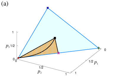
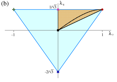
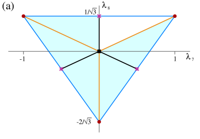
Figure 1: The simplex region in p𝑝p-space (a), and the projection from the p𝑝p-space to the λ𝜆\lambda-space (b), are shown for a 333-level system. In both cases, the vertices representing pure states are indicated by a dot-symbol (occupation probability of the ground state), plus-symbol (occupation probability of the first excited state) and times-symbol (occupation probability of the second excited state). The central square-symbol point represents the most mixed state, and the asterisk-symbol the middle point between p1subscript𝑝1p_{1} and p2subscript𝑝2p_{2}. Solid black lines correspond to the points of the thermal state as a function of the temperature, so the straight line from the vertex corresponds to starting from a pure ground state; the straight line which connects the central point with the middle point along the edge corresponds to the case of two degenerate occupation probabilities of the ground state; and the black curve shows the qualitative behavior for the general case of a density matrix without degenerate eigenvalues.

3 Geometric properties of the qutrit and ququart systems.

To describe the general properties of the qutrit and ququart systems, we use their corresponding diagonal representations. A qutrit system has a geometric representation in a hyperplane of a 333-dimensional space (p𝑝p-space) or in a 222-dimensional space (λ𝜆\lambda- and t𝑡t-spaces), while the ququart system requires of an hyperplane in a 444-dimensional space (p𝑝p-space) or a 333-dimensional space (λ𝜆\lambda- and t𝑡t-space). Here, we review these representations for general diagonal density matrices, i.e., we suppose that the density matrix of the qutrit is given by 𝝆=DiagM(ρ11,ρ22,ρ33)𝝆DiagMsubscript𝜌11subscript𝜌22subscript𝜌33{\bm{\rho}}={\rm DiagM}\,\left(\rho_{11},\,\rho_{22},\,\rho_{33}\right) and for the ququart 𝝆=DiagM(ρ11,ρ22,ρ33,ρ44)𝝆DiagMsubscript𝜌11subscript𝜌22subscript𝜌33subscript𝜌44{\bm{\rho}}={\rm DiagM}\,\left(\rho_{11},\,\rho_{22},\,\rho_{33},\,\rho_{44}\right), and point out some interesting features of their representations.

3.1 Qutrit system

In the probability representation, the numerical eigenvalues are limited by the normalization condition Tr𝝆D=1Trsubscript𝝆𝐷1{\rm Tr}\,{\bm{\rho}}_{D}=1, i.e., p1+p2+p3=1subscript𝑝1subscript𝑝2subscript𝑝31p_{1}+p_{2}+p_{3}=1, and by the probabilistic interpretation of the eigenvalues of the density matrix 0pj10subscript𝑝𝑗10\leq p_{j}\leq 1 (j=1,2,3𝑗123j=1,2,3). The spanned space from these conditions is the simplex shown in Fig. 1(a) whose vertices are located at p1:=(1,0,0)assignsubscript𝑝1100\vec{p}_{1}:=(1,0,0), p2:=(0,1,0)assignsubscript𝑝2010\vec{p}_{2}:=(0,1,0), and p3:=(0,0,1)assignsubscript𝑝3001\vec{p}_{3}:=(0,0,1). These three points depict each one of the pure states (Tr𝝆2=1Trsuperscript𝝆21{\rm Tr}\,{\bm{\rho}}^{2}=1) with one eigenvalue equal to one and the other two equal to zero. The edges delimiting the triangle are parametrized by

pjk=pj+(pkpj)x;x[0,1];j,k=1, 2, 3j<k,formulae-sequencesubscript𝑝𝑗𝑘subscript𝑝𝑗subscript𝑝𝑘subscript𝑝𝑗𝑥formulae-sequence𝑥01𝑗formulae-sequence𝑘123𝑗𝑘\vec{p}_{jk}=\vec{p}_{j}+\left(\vec{p}_{k}-\vec{p}_{j}\right)x\,;\quad x\in[0,1]\,;\quad j,k=1,\,2,\,3\ \land\ j<k\,, (25)

which correspond to all the possible quantum states with one eigenvalue equal to zero. The set of states with at least two equal probability values is parametrized by

pjk=pj+(12[pk+p]pj)x;x[0,1];jkjk,formulae-sequencesubscript𝑝𝑗𝑘subscript𝑝𝑗12delimited-[]subscript𝑝𝑘subscript𝑝subscript𝑝𝑗𝑥formulae-sequence𝑥01𝑗𝑘𝑗𝑘\vec{p}_{jk\ell}=\vec{p}_{j}+\left(\frac{1}{2}\left[\vec{p}_{k}+\vec{p}_{\ell}\right]-\vec{p}_{j}\right)x\,;\quad x\in[0,1]\,;\quad j\neq k\ \land\ j\neq\ell\ \land\ k\neq\ell\,, (26)

and note that pjk=pjksubscript𝑝𝑗𝑘subscript𝑝𝑗𝑘\vec{p}_{jk\ell}=\vec{p}_{j\ell k}. The centroid of the simplex is given by the point pe=(1/3, 1/3, 1/3)subscript𝑝𝑒131313\vec{p}_{e}=(1/3,\,1/3,\,1/3) representing the most mixed state of the system.

The explicit form of the diagonal density matrix operator in the λ𝜆\lambda-space is given by

𝝆=DiagM(13+λ72+λ823,13λ72+λ823,13λ83).𝝆DiagM13subscript𝜆72subscript𝜆82313subscript𝜆72subscript𝜆82313subscript𝜆83{\bm{\rho}}={\rm DiagM}\,\left(\frac{1}{3}+\frac{\lambda_{7}}{2}+\frac{\lambda_{8}}{2\sqrt{3}},\frac{1}{3}-\frac{\lambda_{7}}{2}+\frac{\lambda_{8}}{2\sqrt{3}},\frac{1}{3}-\frac{\lambda_{8}}{\sqrt{3}}\right). (27)

which allows us to describe the system by two variables λ7subscript𝜆7\lambda_{7} and λ8subscript𝜆8\lambda_{8}. For example, the conditions 0ρjj10subscript𝜌𝑗𝑗10\leq\rho_{jj}\leq 1 allow us to define the area of the space in which the values of λ7subscript𝜆7\lambda_{7} and λ8subscript𝜆8\lambda_{8} define a quantum system. These conditions can be written as

1λ71,2+3|λ7|3λ813,formulae-sequence1subscript𝜆7123subscript𝜆73subscript𝜆813-1\leq\lambda_{7}\leq 1,\quad\frac{-2+3|\lambda_{7}|}{\sqrt{3}}\leq\lambda_{8}\leq\frac{1}{\sqrt{3}}, (28)

which defines a triangle with vertices at (1, 1/3131/\sqrt{3}), (-1, 1/3131/\sqrt{3}), and (0, 2/323-2/\sqrt{3}), corresponding to the pure states with density matrices DiagM(1,0,0)DiagM100{\rm DiagM}\,\left(1,0,0\right), DiagM(0,1,0)DiagM010{\rm DiagM}\,\left(0,1,0\right), and DiagM(0,0,1)DiagM001{\rm DiagM}\,\left(0,0,1\right), respectively.

Since the simplexes in p𝑝p-space and λ𝜆\lambda-space are related through a linear map, we consider first these representations, by choosing the diagonal Gell-Mann operators as

𝚲7=DiagM(1,1, 0);𝚲8=13DiagM(1, 1,2).formulae-sequencesubscript𝚲7DiagM11 0subscript𝚲813DiagM112{\bm{\Lambda}}_{7}={\rm DiagM}\,\left(1,\,-1,\,0\right)\,;\qquad{\bm{\Lambda}}_{8}=\frac{1}{\sqrt{3}}{\rm DiagM}\,\left(1,\,1,\,-2\right)\,.

Notice that the Gell-Mann vector is reduced to only two components different from zero. We have the matrix transformation p=𝑴Λ𝑝𝑴Λ\vec{p}={\bm{M}}\vec{\Lambda} with p=(p1,p2,p3)𝑝subscript𝑝1subscript𝑝2subscript𝑝3\vec{p}=(p_{1},\,p_{2},\,p_{3}), Λ=(λ7,λ8, 1)Λsubscript𝜆7subscript𝜆81\vec{\Lambda}=(\lambda_{7},\,\lambda_{8},\,1) and

𝑴=12(113231132302323);𝑴1=(110131323111);formulae-sequence𝑴12113231132302323superscript𝑴1110131323111{\bm{M}}=\frac{1}{2}\left(\begin{array}[]{c c c}1&\frac{1}{\sqrt{3}}&\frac{2}{3}\\ -1&\frac{1}{\sqrt{3}}&\frac{2}{3}\\ 0&-\frac{2}{\sqrt{3}}&\frac{2}{3}\end{array}\right)\,;\qquad{\bm{M}}^{-1}=\left(\begin{array}[]{c c c}1&-1&0\\ \frac{1}{\sqrt{3}}&\frac{1}{\sqrt{3}}&-\frac{2}{\sqrt{3}}\\ 1&1&1\end{array}\right)\,; (29)

the two dimensional λ𝜆\lambda-space is given by the points λ:=(λ7,λ8)assign𝜆subscript𝜆7subscript𝜆8\vec{\lambda}:=(\lambda_{7},\,\lambda_{8}), so the vertices in the plimit-from𝑝p-simplex are changed to vertices in the λ𝜆\lambda-space as

p1Λ1=(1,13, 1);p2Λ2=(1,13, 1);p3Λ3=(0,23, 1);formulae-sequencesubscript𝑝1subscriptΛ11131subscript𝑝2subscriptΛ21131subscript𝑝3subscriptΛ30231\vec{p}_{1}\to\vec{\Lambda}_{1}=\left(1,\frac{1}{\sqrt{3}},\,1\right)\,;\quad\vec{p}_{2}\to\vec{\Lambda}_{2}=\left(-1,\frac{1}{\sqrt{3}},\,1\right)\,;\quad\vec{p}_{3}\to\vec{\Lambda}_{3}=\left(0,-\frac{2}{\sqrt{3}},\,1\right)\,;

and an arbitrary point by

pΛ=(p1p2,13p33, 1).𝑝Λsubscript𝑝1subscript𝑝213subscript𝑝331\vec{p}\to\vec{\Lambda}=\left(p_{1}-p_{2},\,\frac{1-3p_{3}}{\sqrt{3}},\,1\right)\,.

In figure 1 we show the values which yield a physical state of the system, both in the simplex Fig. 1(a) and the λ𝜆\lambda-space Fig. 1(b). In both cases the vertices of the triangle correspond to pure states of the system. By considering that the three levels represent an atomic or molecular system and give the level occupation probabilities, we use the following convention: the ground state is indicated by p1subscript𝑝1\vec{p}_{1} or λ1subscript𝜆1\vec{\lambda}_{1} (red dot in the figure), the first excited state by p2subscript𝑝2\vec{p}_{2} or λ2subscript𝜆2\vec{\lambda}_{2} (plus-symbol in the figure), and the second excited state by p3subscript𝑝3\vec{p}_{3} or λ3subscript𝜆3\vec{\lambda}_{3} (times-symbol in the figure).

Other points of interest are the thermal endpoints corresponding to the most mixed state pe=(p1+p2+p3)/3subscript𝑝𝑒subscript𝑝1subscript𝑝2subscript𝑝33\vec{p}_{e}=(\vec{p}_{1}+\vec{p}_{2}+\vec{p}_{3})/3 or λe=(λ1+λ2+λ3)/3=(0,0)subscript𝜆𝑒subscript𝜆1subscript𝜆2subscript𝜆3300\vec{\lambda}_{e}=(\vec{\lambda}_{1}+\vec{\lambda}_{2}+\vec{\lambda}_{3})/3=(0,0) (square-symbol in the figure), and the cases when two occupation probabilities of the three-level system are equal (i.e., two eigenvalues of the density matrix are degenerate): pm=(pi+pj)/2subscript𝑝𝑚subscript𝑝𝑖subscript𝑝𝑗2\vec{p}_{m}=(\vec{p}_{i}+\vec{p}_{j})/2 or λm=(λi+λj)/2subscript𝜆𝑚subscript𝜆𝑖subscript𝜆𝑗2\vec{\lambda}_{m}=(\vec{\lambda}_{i}+\vec{\lambda}_{j})/2, ij𝑖𝑗i\neq j (asterisk-symbol in the figure).

The open (shaded) internal triangle establishes the case without degeneracy, corresponding to the set of points in the simplex for a thermal density matrix; the black lines connecting the point pesubscript𝑝𝑒\vec{p}_{e} (λesubscript𝜆𝑒\vec{\lambda}_{e}) with either the vertex p1subscript𝑝1\vec{p}_{1} (λ1subscript𝜆1\vec{\lambda}_{1}) or the middle point pmsubscript𝑝𝑚\vec{p}_{m} (λmsubscript𝜆𝑚\vec{\lambda}_{m}) correspond to trajectories from the pure ground state and from the case of a degenerate ground state with two equal occupation probabilities, respectively. The qualitative behavior of the thermal density matrix as a function of the temperature, for the non-degenerate case, is shown by the black curve in the figure, whose concavity increases when the first excited state occupation probability of the system approaches that of the ground state.
Refer to caption
Refer to caption
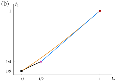
Figure 2: Non-linear map from (a) λ𝜆\lambda-space to (b) t𝑡t-space. The pure states (dot-symbol) are mapped onto the vertex t1subscript𝑡1\vec{t}_{1} (dot-symbol), the middle-points (asterisk-symbol) onto the vertex t2subscript𝑡2\vec{t}_{2} (asterisk-symbol) and the most mixed state (square-symbol) onto the vertex t3subscript𝑡3\vec{t}_{3} (square-symbol). Each straight-line segment which connects any two indicated points in λ𝜆\lambda-space is mapped to a boundary-curve in the t𝑡t-space, and each open triangle (as the white triangle) is mapped onto the interior of the bounded region in t𝑡t-space.

Now, we consider the non-linear map from the λ𝜆\lambda-space to the t𝑡t-space (cf. Fig. 2). As pointed out above, this map does not distinguish between pure states, and hence each point in t𝑡t-space represents a set of physical states. In particular, the pure states λpsubscript𝜆𝑝\vec{\lambda}_{p} (dot-symbol) at the vertices, middle points λmsubscript𝜆𝑚\vec{\lambda}_{m} (asterisk-symbol), and the most mixed state λesubscript𝜆𝑒\vec{\lambda}_{e} (square-symbol) indicated in Fig. 2(a) are mapped to the points

λpt1=(1,1);λmt2=(12,14);λet3=(13,19),formulae-sequencesubscript𝜆𝑝subscript𝑡111subscript𝜆𝑚subscript𝑡21214subscript𝜆𝑒subscript𝑡31319\vec{\lambda}_{p}\to\vec{t}_{1}=(1,1)\,;\quad\vec{\lambda}_{m}\to\vec{t}_{2}=\left(\frac{1}{2},\,\frac{1}{4}\right)\,;\quad\vec{\lambda}_{e}\to\vec{t}_{3}=\left(\frac{1}{3},\,\frac{1}{9}\right)\,,

indicated with the same symbols in Fig. 2(b). Any point λ=(λ7,λ8)𝜆subscript𝜆7subscript𝜆8\vec{\lambda}=(\lambda_{7},\,\lambda_{8}) in λ𝜆\lambda-space is mapped to a point t=(t2,t3)𝑡subscript𝑡2subscript𝑡3\vec{t}=(t_{2},\,t_{3}) via the transformation

λt=(13+12(λ72+λ82),19+λ724(2+3λ8)+λ8243(23λ8)).𝜆𝑡1312superscriptsubscript𝜆72superscriptsubscript𝜆8219superscriptsubscript𝜆72423subscript𝜆8superscriptsubscript𝜆824323subscript𝜆8\vec{\lambda}\to\vec{t}=\left(\frac{1}{3}+\frac{1}{2}\left(\lambda_{7}^{2}+\lambda_{8}^{2}\right),\,\frac{1}{9}+\frac{\lambda_{7}^{2}}{4}\left(2+\sqrt{3}\lambda_{8}\right)+\frac{\lambda_{8}^{2}}{4\sqrt{3}}\left(2\sqrt{3}-\lambda_{8}\right)\right)\,.

The straight line segments connecting points in the λ𝜆\lambda-space, shown in Fig. 2(a), can be parametrized as follows:

λjepsubscriptsuperscript𝜆𝑒𝑝𝑗\displaystyle\vec{\lambda}^{ep}_{j} =\displaystyle= λjx;λjkem=12(λj+λk)x;x[0,1],formulae-sequencesubscript𝜆𝑗𝑥subscriptsuperscript𝜆𝑒𝑚𝑗𝑘12subscript𝜆𝑗subscript𝜆𝑘𝑥𝑥01\displaystyle\vec{\lambda}_{j}\,x\,;\qquad\vec{\lambda}^{em}_{jk}=\frac{1}{2}\left(\vec{\lambda}_{j}+\vec{\lambda}_{k}\right)\,x\,;\quad x\in[0,1]\,,
λjkmpsuperscriptsubscript𝜆𝑗𝑘𝑚𝑝\displaystyle\vec{\lambda}_{jk}^{mp} =\displaystyle= λj+(λkλj)x;x[12,1],subscript𝜆𝑗subscript𝜆𝑘subscript𝜆𝑗𝑥𝑥121\displaystyle\vec{\lambda}_{j}+\left(\vec{\lambda}_{k}-\vec{\lambda}_{j}\right)\,x\,;\quad x\in\left[\frac{1}{2},1\right]\,,

for j,k=1,2,3formulae-sequence𝑗𝑘123j,k=1,2,3, with the upper-indices indicating the corresponding connected points: most mixed state (e𝑒e), middle point of two occupation probabilities (m𝑚m), and pure states (p)𝑝(p). Each path maps onto a trajectory in t𝑡t-space corresponding to their boundaries. Any point in t𝑡t-space lying within these trajectories is physically aceptable (and only those), since the density matrix is given in a diagonal form. After the transformation these segments will be given by (see Fig. 2(b))

t1epsuperscriptsubscript𝑡1𝑒𝑝\displaystyle\vec{t}_{1}^{\ ep} =\displaystyle= 19(3+6x2, 1+6x2+2x3);x[0,1],1936superscript𝑥216superscript𝑥22superscript𝑥3𝑥01\displaystyle\frac{1}{9}\left(3+6x^{2},\,1+6x^{2}+2x^{3}\right)\,;\quad x\in[0,1]\,,
t12emsuperscriptsubscript𝑡12𝑒𝑚\displaystyle\vec{t}_{12}^{\ em} =\displaystyle= 13(1+x22,13+x22x312);x[0,1],131superscript𝑥2213superscript𝑥22superscript𝑥312𝑥01\displaystyle\frac{1}{3}\left(1+\frac{x^{2}}{2},\,\frac{1}{3}+\frac{x^{2}}{2}-\frac{x^{3}}{12}\right)\,;\quad x\in[0,1]\,,
t21mpsuperscriptsubscript𝑡21𝑚𝑝\displaystyle\vec{t}_{21}^{\ mp} =\displaystyle= (12x+2x2, 13x+x2);x[12,1].12𝑥2superscript𝑥213𝑥superscript𝑥2𝑥121\displaystyle\left(1-2x+2x^{2},\,1-3x+x^{2}\right)\,;\quad x\in\left[\frac{1}{2},1\right]\,.

Notice that the open internal triangle in the λ𝜆\lambda-space [white triangle in Figure 2(a)], representing the domain of thermal states as was discussed previously [cf. Figs. 1(b) and 2(a)], is mapped onto the full open region in t𝑡t-space bounded by the trajectories shown. In fact, all points t𝑡\vec{t} with exception of the boundary that connects the vertices t1subscript𝑡1\vec{t}_{1} and t2subscript𝑡2\vec{t}_{2} may be associated to a thermal state. The same happens for all other triangles in the λ𝜆\lambda-space.

The non-linear map from the Gell-Mann variables to the invariants representation has been given above; however it is interesting to determine the set of density matrices with equal invariants, i.e., the set with equal t2=Tr[𝝆2]subscript𝑡2Trdelimited-[]superscript𝝆2t_{2}={\rm Tr}\,[{\bm{\rho}}^{2}] (purity), or with t3=Tr[𝝆3]subscript𝑡3Trdelimited-[]superscript𝝆3t_{3}={\rm Tr}\,[{\bm{\rho}}^{3}] a constant value. The first condition p12+p22+p32=t2superscriptsubscript𝑝12superscriptsubscript𝑝22superscriptsubscript𝑝32subscript𝑡2p_{1}^{2}+p_{2}^{2}+p_{3}^{2}=t_{2} gives a circumference centered at pesubscript𝑝𝑒\vec{p}_{e} on the simplex, which can be parametrized by

pt2=pe+3t213(𝒑1ecos(α)+𝒒1esin(α));α[0,2π],formulae-sequencesubscript𝑝subscript𝑡2subscript𝑝𝑒3subscript𝑡213subscript𝒑1𝑒𝛼subscript𝒒1𝑒𝛼𝛼02𝜋\vec{p}_{t_{2}}=\vec{p}_{e}+\sqrt{\frac{3t_{2}-1}{3}}\left({\bm{p}}_{1e}\cos(\alpha)+{\bm{q}}_{1e}\sin(\alpha)\right)\,;\quad\alpha\in\left[0,2\pi\right]\,, (30)

with the constraint

13t21,13subscript𝑡21\frac{1}{3}\leq t_{2}\leq 1\,,

and where we have chosen the unit vectors

𝒑1e:=p1pep1pe;𝒒1e:=pe×p1pe×p1.formulae-sequenceassignsubscript𝒑1𝑒subscript𝑝1subscript𝑝𝑒normsubscript𝑝1subscript𝑝𝑒assignsubscript𝒒1𝑒subscript𝑝𝑒subscript𝑝1normsubscript𝑝𝑒subscript𝑝1{\bm{p}}_{1e}:=\frac{\vec{p}_{1}-\vec{p}_{e}}{||\vec{p}_{1}-\vec{p}_{e}||}\,;\qquad{\bm{q}}_{1e}:=\frac{\vec{p}_{e}\times\vec{p}_{1}}{||\vec{p}_{e}\times\vec{p}_{1}||}\,.

The case t3subscript𝑡3t_{3} constant is given by the set of points of the form

pt3=pe+r(t3,α)(𝒑1ecos(α)+𝒒1esin(α));α[0,2π],formulae-sequencesubscript𝑝subscript𝑡3subscript𝑝𝑒𝑟subscript𝑡3𝛼subscript𝒑1𝑒𝛼subscript𝒒1𝑒𝛼𝛼02𝜋\vec{p}_{t_{3}}=\vec{p}_{e}+r(t_{3},\alpha)\left({\bm{p}}_{1e}\cos(\alpha)+{\bm{q}}_{1e}\sin(\alpha)\right)\,;\quad\alpha\in\left[0,2\pi\right]\,, (31)

where r(t3,α)𝑟subscript𝑡3𝛼r(t_{3},\alpha) satisfies

19+r2+cos(3α)6r3=t3,19superscript𝑟23𝛼6superscript𝑟3subscript𝑡3\frac{1}{9}+r^{2}+\frac{\cos(3\alpha)}{\sqrt{6}}r^{3}=t_{3}\,,

and the constraints for having physical states are

19t31,0r23.formulae-sequence19subscript𝑡310𝑟23\frac{1}{9}\leq t_{3}\leq 1\,,\qquad 0\leq r\leq\sqrt{\frac{2}{3}}\,.

The latter are obtained by using the boundaries of the invariant t2subscript𝑡2t_{2} and the fact that r𝑟r is the radius in a polar coordinate vector representation, so that pt3subscript𝑝subscript𝑡3\vec{p}_{t_{3}} is a single-valued vector function of α𝛼\alpha. Additional to these constraints, we know that only the points of the simplex represent physical states, i.e., p1+p2+p3=1subscript𝑝1subscript𝑝2subscript𝑝31p_{1}+p_{2}+p_{3}=1.

In the λ𝜆\lambda-space the same set of trajectories are obtained from the linear map Λ=𝑴1pΛsuperscript𝑴1𝑝\vec{\Lambda}={\bm{M}}^{-1}\vec{p}\, with 𝑴𝑴{\bm{M}} given in Eq. (29). So the parametric curves in the λ𝜆\lambda-space read: Λjk=𝑴1pjksubscriptΛ𝑗𝑘superscript𝑴1subscript𝑝𝑗𝑘\vec{\Lambda}_{jk}={\bm{M}}^{-1}\vec{p}_{jk}, Λjk=𝑴1pjksubscriptΛ𝑗𝑘superscript𝑴1subscript𝑝𝑗𝑘\vec{\Lambda}_{jk\ell}={\bm{M}}^{-1}\vec{p}_{jk\ell}, Λt2=𝑴1pt2subscriptΛsubscript𝑡2superscript𝑴1subscript𝑝subscript𝑡2\vec{\Lambda}_{t_{2}}={\bm{M}}^{-1}\vec{p}_{t_{2}} and Λt3=𝑴1pt3subscriptΛsubscript𝑡3superscript𝑴1subscript𝑝subscript𝑡3\vec{\Lambda}_{t_{3}}={\bm{M}}^{-1}\vec{p}_{t_{3}}, respectively.

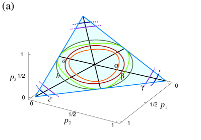
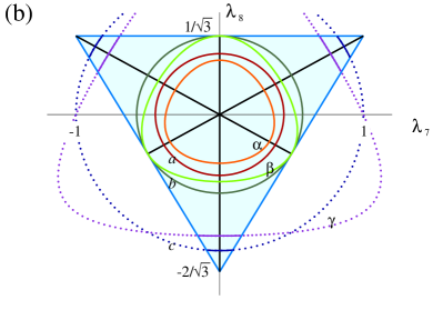
In figure 3, one can see all the characteristics mentioned above for the qutrit system in the p𝑝p-space, Fig. 3(a), and in the λ𝜆\lambda-space, Fig. 3(b). The edges of the simplex given by Eq. (25) represent the set of density matrices with at least one of their eigenvalues equal to zero; the medians of the triangle (black lines) parametrized by Eq. (26) correspond to the set of density matrices with at least two degenerate eigenvalues; the curves (or segments of curve thereof) inside the simplex represent the set of states with one invariant constant. For t2subscript𝑡2t_{2}, corresponding to circles with center at the most mixed state Eq. (30), we have labeled a few cases: (a)𝑎(a) for t2=13/30subscript𝑡21330t_{2}=13/30, (b)𝑏(b) for t2=1/2subscript𝑡212t_{2}=1/2, and (c)𝑐(c) for t2=5/6subscript𝑡256t_{2}=5/6. For t3subscript𝑡3t_{3} constant Eq. (31) we have trajectories that look like triangles with rounded vertices (resembling a Reuleaux triangle) centered at the most mixed state, and we have labeled: (α𝛼\alpha) for t3=109/600subscript𝑡3109600t_{3}=109/600, (β𝛽\beta) for t3=1/4subscript𝑡314t_{3}=1/4, and (γ𝛾\gamma) for t3=11/18subscript𝑡31118t_{3}=11/18. In both cases we may see the continuation out the simplex (unphysical states) of the broken trajectories, drawn with dots, in order to illustrate the shape of the full curve in the whole space.
Refer to caption
Refer to caption
Figure 3: Simplex in the p𝑝p-space (a), and affine λ𝜆\lambda-space (b). The edges of the simplex given by Eq. (25) correspond to states with at least one eigenvalue equal to cero; the medians of the triangle given by Eq. (26) contain states with at least two eigenvalues equal to zero; the centered circles given by Eq. (30) represent the set of density matrices with equal purity (invariant t2subscript𝑡2t_{2}), shown for the values t2=13/30,1/2,5/6subscript𝑡213301256t_{2}=13/30,1/2,5/6 (labeled by a,b𝑎𝑏a,\,b and c𝑐c, respectively); while the triangles with rounded vertices given by Eq. (31) represent the set of density matrices with fixed invariant t3subscript𝑡3t_{3}, here shown for the values t3=109/600,1/4,11/18subscript𝑡3109600141118t_{3}=109/600,1/4,11/18 (labeled by α,β𝛼𝛽\alpha,\,\beta and γ𝛾\gamma, respectively). The corresponding ones, via the linear transformation, are show at right in the λ𝜆\lambda-space.
Refer to caption
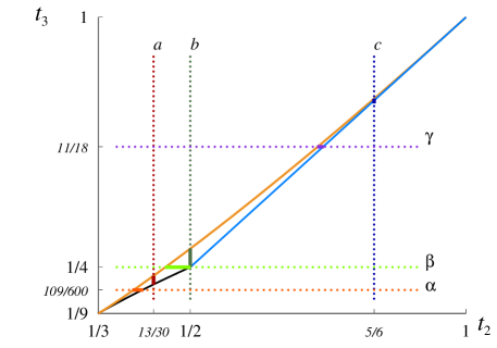
Figure 4: Physical region in t𝑡t-space obtained via the non-linear map from the simplex in the p𝑝p-space or the affine domain in the λ𝜆\lambda-space [Eqs. (25)–(31)]. The image of the curves in Figure 3 carry the same labels here. The unphysical states along the constant dotted lines are drawn for the purpose of clarity. The boundary of the region is given by t3=t229±(3t21)3/292subscript𝑡3plus-or-minussubscript𝑡229superscript3subscript𝑡213292t_{3}=t_{2}-\frac{2}{9}\pm\frac{(3t_{2}-1)^{3/2}}{9\sqrt{2}}, (upper (orange) and short lower (black) lines respectively) and are associated to density matrices with two equal eigenvalues, while the long lower (blue) curve is described by t3=12(3t21)subscript𝑡3123subscript𝑡21t_{3}=\frac{1}{2}(3t_{2}-1) and is associated to density matrices with an eigenvalue equal to zero.

Now for the non linear map from the λ𝜆\lambda-space to the t𝑡t-space. The centered circumferences in the λ𝜆\lambda-space or p𝑝p-space map onto vertical cutoff lines in the t𝑡t-space, while the kind of trajectories given by Eq. (31), which resemble a kind of Reuleaux triangle, map onto horizontal cutoff lines in the t𝑡t-space. These are shown in Figure 4, where we have labeled the trajectories in a similar fashion to Figure 3. For clarity, we have extended the trajectories out of the physical region with dotted lines; the counterpart to these extensions, which are unphysical, do not appear in the non-linear map of a single inscribed curve in the affine domain of the λ𝜆\lambda-space, since any inscribed curve in the affine domain maps to a curve in the physical t𝑡t-space. The boundary of the compact region in Figure 4 corresponds to the edges and medians of the triangle (see Fig. 2), i.e., they are composed by states with at least one vanishing eigenvalue (vertices and edges of the triangle in the p𝑝p- or λ𝜆\lambda-space) and states with degenerate eigenvalues (medians of the triangle in the p𝑝p- or λ𝜆\lambda-space).

Summarizing, we have represented a qutrit by a 3×3333\times 3 matrix yielding three eigenvalues in its diagonal representation, i.e., 𝝆D=DiagM(p1,p2,p3)subscript𝝆𝐷DiagMsubscript𝑝1subscript𝑝2subscript𝑝3{\bm{\rho}}_{D}={\rm DiagM}\,\left(p_{1},p_{2},p_{3}\right). The diagonal state can be studied in several ways, by examining directly the three eigenvalues (p𝑝p-space), equivalently in a 222-dimensional λ𝜆\lambda-space by using the Gell-Mann parametrization, or by exploring the invariants of the density matrix t2=Tr𝝆D2subscript𝑡2Trsuperscriptsubscript𝝆𝐷2t_{2}={\rm Tr}\,{\bm{\rho}}_{D}^{2} and t3=Tr𝝆D3subscript𝑡3Trsuperscriptsubscript𝝆𝐷3t_{3}={\rm Tr}\,{\bm{\rho}}_{D}^{3} (t𝑡t-space).

3.2 Ququart system

Refer to caption
Refer to caption
Refer to caption
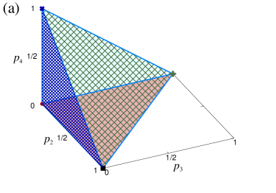
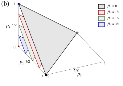
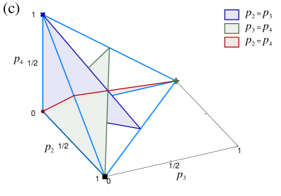
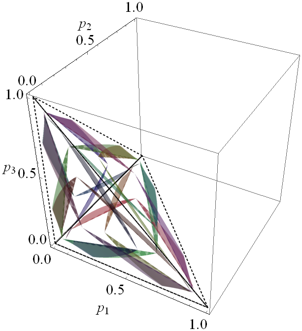
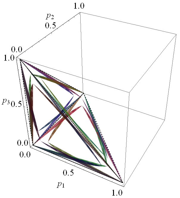
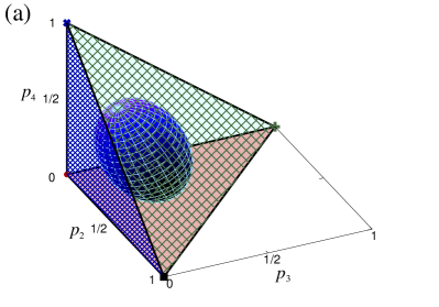
Figure 5: Simplex for a ququart system in p𝑝p-space. (a) Solid region in the subspace {p2,p3,p4}subscript𝑝2subscript𝑝3subscript𝑝4\{p_{2},\,p_{3},\,p_{4}\}; (b) the simplex for fixed values of probability p1subscript𝑝1p_{1}; and (c) the cut planes when two probabilities take the same value. In all cases the pure states are indicated by dot-symbols for 𝝆1subscript𝝆1{\bm{\rho}}_{1}, square-symbols for 𝝆2subscript𝝆2{\bm{\rho}}_{2}, plus-symbols for 𝝆3subscript𝝆3{\bm{\rho}}_{3} and times-symbols for 𝝆4subscript𝝆4{\bm{\rho}}_{4}.

The diagonal density matrix of a ququart system is given in p𝑝p-space as Eq. (20)

𝝆=DiagM(p1,p2,p3,p4)=DiagM(p),𝝆DiagMsubscript𝑝1subscript𝑝2subscript𝑝3subscript𝑝4DiagM𝑝{\bm{\rho}}={\rm DiagM}\,\left(p_{1},\,p_{2},\,p_{3},\,p_{4}\right)={\rm DiagM}\,\left(\vec{p}\right)\,,

its 333-simplex in U(4)U4{\rm U}(4) is a tetrahedron with vertices at 𝝆j=DiagM(pj)subscript𝝆𝑗DiagMsubscript𝑝𝑗{\bm{\rho}}_{j}={\rm DiagM}\,\left(\vec{p}_{j}\right) for which pj=1subscript𝑝𝑗1p_{j}=1. It can be visualized as a solid in 333-dimensional space, generated by the probabilities p2,p3subscript𝑝2subscript𝑝3p_{2},\,p_{3} and p4subscript𝑝4p_{4}, with p1=1p2p3p4subscript𝑝11subscript𝑝2subscript𝑝3subscript𝑝4p_{1}=1-p_{2}-p_{3}-p_{4} as in figure 5(a). Its vertices, indicated by dot-, square-, plus- and times-symbols, correspond to pure states; according to 𝝆j=DiagM(pj)subscript𝝆𝑗DiagMsubscript𝑝𝑗{\bm{\rho}}_{j}={\rm DiagM}\,\left(\vec{p}_{j}\right) these are denoted by 𝝆1,𝝆2,𝝆3subscript𝝆1subscript𝝆2subscript𝝆3{\bm{\rho}}_{1},\,{\bm{\rho}}_{2},\,{\bm{\rho}}_{3} and 𝝆4subscript𝝆4{\bm{\rho}}_{4}. The faces correspond to the set of points where at least one eigenvalue is zero, while at the edges at least two eigenvalues vanish. Therefore one has double degeneracy corresponding (as a limit case, see discussion below) to the orbits in U(4)U4{\rm U}(4) of dimension 6, associated to the quotient group U(4)/(U(2)U(1)U(1))U4tensor-producttensor-productU2U1U1{\rm U}(4)/\left({\rm U}(2)\otimes{\rm U}(1)\otimes{\rm U}(1)\right). For a fixed value of p1subscript𝑝1p_{1} the set given by

p2+p3+p4=c0;c:=1p1,formulae-sequencesubscript𝑝2subscript𝑝3subscript𝑝4𝑐0assign𝑐1subscript𝑝1p_{2}+p_{3}+p_{4}=c\geq 0\,;\qquad c:=1-p_{1}\,,

defines a region similar to that in the case of the qutrit [cf. Fig. 1(a)] which grows as p10subscript𝑝10p_{1}\to 0 (cf. Fig. 5(b)). The case when two probability values are equal, given by the condition

pj+pk+2p=1,pm=p,formulae-sequencesubscript𝑝𝑗subscript𝑝𝑘2subscript𝑝1subscript𝑝𝑚subscript𝑝p_{j}+p_{k}+2p_{\ell}=1\,,\qquad p_{m}=p_{\ell}\,,

cuts the simplex at a plane; the cases pm=psubscript𝑝𝑚subscript𝑝p_{m}=p_{\ell} with m1𝑚1m\neq 1 and 11\ell\neq 1 are shown in figure 5(c). These planes in turn generate the medians of the triangular face for a constant value p1subscript𝑝1p_{1}. The most mixed state is given by the point

pe:=14(1, 1, 1, 1).assignsubscript𝑝𝑒141111\vec{p}_{e}:=\frac{1}{4}\left(1,\,1,\,1,\,1\right)\,.

Using this, one may parametrize each point of the simplex in the p𝑝p-space as

p=pe+r2[cos(ϕ)sin(θ)e^1+sin(ϕ)sin(θ)e^2+cos(θ)e^3],𝑝subscript𝑝𝑒𝑟2delimited-[]italic-ϕ𝜃subscript^𝑒1italic-ϕ𝜃subscript^𝑒2𝜃subscript^𝑒3\vec{p}=\vec{p}_{e}+\frac{r}{\sqrt{2}}\left[\cos(\phi)\sin(\theta)\hat{e}_{1}+\sin(\phi)\sin(\theta)\hat{e}_{2}+\cos(\theta)\hat{e}_{3}\right]\,, (32)

with r0,ϕ[0, 2π]formulae-sequence𝑟0italic-ϕ02𝜋r\geq 0,\phi\in[0,\,2\pi] and θ[0,π]𝜃0𝜋\theta\in[0,\,\pi] and where the unitary vectors are given by

e^1subscript^𝑒1\displaystyle\hat{e}_{1} =\displaystyle= 12(1,1, 0, 0);e^2=16(1, 1,2, 0);1211 0 0subscript^𝑒216112 0\displaystyle\frac{1}{\sqrt{2}}\left(1,\,-1,\,0,\,0\right)\,;\qquad\hat{e}_{2}=\frac{1}{\sqrt{6}}\left(1,\,1,\,-2,\,0\right)\,;
e^3subscript^𝑒3\displaystyle\hat{e}_{3} =\displaystyle= 36(1, 1, 1,3).361113\displaystyle\frac{\sqrt{3}}{6}\left(1,\,1,\,1,\,-3\right)\,.

The advantage of writing the point in the simplex in this form is to obtain the invariants in terms of the radial and polar variables, so a density matrix which is written in a general form as 𝝆=DiagM(p)𝝆DiagM𝑝{\bm{\rho}}={\rm DiagM}\,\left(\vec{p}\right) has the invariants written simply as

t2subscript𝑡2\displaystyle t_{2} =\displaystyle= 14(1+2r2);t3=116+38r2+a396r3;1412superscript𝑟2subscript𝑡311638superscript𝑟2subscript𝑎396superscript𝑟3\displaystyle\frac{1}{4}\left(1+2r^{2}\right)\,;\qquad t_{3}=\frac{1}{16}+\frac{3}{8}r^{2}+\frac{a_{3}}{96}r^{3}\,;
t4subscript𝑡4\displaystyle t_{4} =\displaystyle= 164+316r2+a396r3+b4384r4,164316superscript𝑟2subscript𝑎396superscript𝑟3subscript𝑏4384superscript𝑟4\displaystyle\frac{1}{64}+\frac{3}{16}r^{2}+\frac{a_{3}}{96}r^{3}+\frac{b_{4}}{384}r^{4}\,, (33)

where we have used

a3subscript𝑎3\displaystyle a_{3} :=assign\displaystyle:= 6[3cos(θ)+5cos(3θ)]+83sin3(θ)sin(3ϕ);6delimited-[]3𝜃53𝜃83superscript3𝜃3italic-ϕ\displaystyle-\sqrt{6}\left[3\cos(\theta)+5\cos(3\theta)\right]+8\sqrt{3}\sin^{3}(\theta)\sin(3\phi)\,;
b4subscript𝑏4\displaystyle b_{4} :=assign\displaystyle:= 45+4cos(2θ)+7cos(4θ)+322cos(θ)sin3(θ)sin(3ϕ),4542𝜃74𝜃322𝜃superscript3𝜃3italic-ϕ\displaystyle 45+4\cos(2\theta)+7\cos(4\theta)+32\sqrt{2}\cos(\theta)\sin^{3}(\theta)\sin(3\phi)\,,

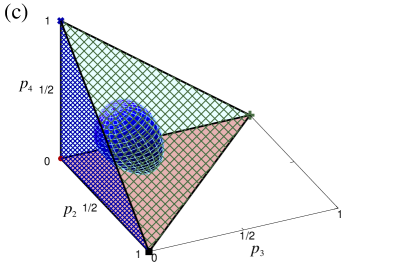
to simplify the notation. Thus, in the p𝑝p-space the condition t2subscript𝑡2t_{2} constant yields a hyper-sphere of radius r=4t21/2𝑟4subscript𝑡212r=\sqrt{4t_{2}-1}/2 centred at pesubscript𝑝𝑒\vec{p}_{e}. On the simplex, represented by the coordinate axes p2,p3subscript𝑝2subscript𝑝3p_{2},\,p_{3} and p4subscript𝑝4p_{4}, this hyper-sphere is seen elongated: at the limit values of t2subscript𝑡2t_{2} one obtains the point pesubscript𝑝𝑒\vec{p}_{e} (t2=1/4subscript𝑡214t_{2}=1/4) and a surface which intersects the simplex only at the vertices (t2=1subscript𝑡21t_{2}=1); intermediate values generate a surface lying completely inside the simplex. Figure 6 shows this for different values of t2subscript𝑡2t_{2}: (a) t2=1/3subscript𝑡213t_{2}=1/3; (b) t2=1/2subscript𝑡212t_{2}=1/2. Points outside the simplex correspond to unphysical states.
Refer to caption
Refer to caption
Refer to caption
Refer to caption
Refer to caption
Refer to caption
Figure 6: Surfaces defined on the 3limit-from33-simplex for the ququart when the invariants of SU(4)SU4{\rm SU}(4) take a constant value: (a) t2=1/3subscript𝑡213t_{2}=1/3, (b) t2=1/2subscript𝑡212t_{2}=1/2, (c) t3=1/10subscript𝑡3110t_{3}=1/10, (d) t3=7/40subscript𝑡3740t_{3}=7/40 (e) t4=1/32subscript𝑡4132t_{4}=1/32 and (f) t4=5/64subscript𝑡4564t_{4}=5/64. Points outside the simplex correspond to unphysical states.
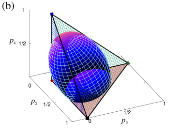
Solving for t3subscript𝑡3t_{3} and t4subscript𝑡4t_{4} in terms of r0𝑟0r\geq 0 one finds the parametric form of the surfaces of constant value for each of the invariants. In both cases one has a symmetry of 2π/32𝜋32\pi/3 in the angular variable ϕitalic-ϕ\phi as expected by the form of the coefficients a3subscript𝑎3a_{3} and b4subscript𝑏4b_{4}. These surfaces are shown in Figure 6, (c) for t3=1/10subscript𝑡3110t_{3}=1/10, (d) for t3=7/40subscript𝑡3740t_{3}=7/40, (e) for t4=1/32subscript𝑡4132t_{4}=1/32 and (f) for t4=5/64subscript𝑡4564t_{4}=5/64.

The explicit density matrix in the λ𝜆\lambda-space can be written as

𝝆=DiagM(14+λ132+λ1423+λ1526,14λ132+λ1423+λ1526,14λ143+λ1526,143λ1526).𝝆DiagM14subscript𝜆132subscript𝜆1423subscript𝜆152614subscript𝜆132subscript𝜆1423subscript𝜆152614subscript𝜆143subscript𝜆1526143subscript𝜆1526{\bm{\rho}}={\rm DiagM}\,\left(\frac{1}{4}+\frac{\lambda_{13}}{2}+\frac{\lambda_{14}}{2\sqrt{3}}+\frac{\lambda_{15}}{2\sqrt{6}},\ \frac{1}{4}-\frac{\lambda_{13}}{2}+\frac{\lambda_{14}}{2\sqrt{3}}+\frac{\lambda_{15}}{2\sqrt{6}},\ \frac{1}{4}-\frac{\lambda_{14}}{\sqrt{3}}+\frac{\lambda_{15}}{2\sqrt{6}},\ \frac{1}{4}-\frac{3\lambda_{15}}{2\sqrt{6}}\right)\,. (34)

Since the density matrix is positive semi-definite 0ρjj10subscript𝜌𝑗𝑗10\leq\rho_{jj}\leq 1 (j=1,,4𝑗14j=1,\ldots,4), we have a tetrahedron given by

1λ131,23λ1413,23λ1516.formulae-sequence1subscript𝜆13123subscript𝜆141323subscript𝜆1516-1\leq\lambda_{13}\leq 1,\quad-\frac{2}{\sqrt{3}}\leq\lambda_{14}\leq\frac{1}{\sqrt{3}},\quad-\sqrt{\frac{2}{3}}\leq\lambda_{15}\leq\frac{1}{\sqrt{6}}. (35)

The pure states, corresponding to the density matrices 𝝆=diag(1,0,0,0)𝝆diag1000{\bm{\rho}}={\rm diag}(1,0,0,0), 𝝆=diag(0,1,0,0)𝝆diag0100{\bm{\rho}}={\rm diag}(0,1,0,0), 𝝆=diag(0,0,1,0)𝝆diag0010{\bm{\rho}}={\rm diag}(0,0,1,0), and 𝝆=diag(0,0,0,1)𝝆diag0001{\bm{\rho}}={\rm diag}(0,0,0,1), are associated to the vertices (1,13,16)11316\left(1,\frac{1}{\sqrt{3}},\frac{1}{\sqrt{6}}\right), (1,13,16)11316\left(-1,\frac{1}{\sqrt{3}},\frac{1}{\sqrt{6}}\right), (0,23,16)02316\left(0,-\frac{2}{\sqrt{3}},\frac{1}{\sqrt{6}}\right), and (0,0,23)0023\left(0,0,-\sqrt{\frac{2}{3}}\right), respectively. The values for λ13subscript𝜆13\lambda_{13}, λ14subscript𝜆14\lambda_{14}, λ15subscript𝜆15\lambda_{15} on the faces of the tetrahedron correspond to pure states, while the centroid corresponds to the most mixed state with 𝝆=diag(1/4,1/4,1/4,1/4)𝝆diag14141414{\bm{\rho}}={\rm diag}(1/4,1/4,1/4,1/4).

To visualise the thermal region it is convenient to consider the Gell-Mann representation, by choosing the diagonal matrices as

𝚲13subscript𝚲13\displaystyle{\bm{\Lambda}}_{13} =\displaystyle= DiagM(1,1, 0, 0);𝚲14=13DiagM(1, 1,2, 0);DiagM11 0 0subscript𝚲1413DiagM112 0\displaystyle{\rm DiagM}\,\left(1,\,-1,\,0,\,0\right)\,;\qquad{\bm{\Lambda}}_{14}=\frac{1}{\sqrt{3}}{\rm DiagM}\,\left(1,\,1,\,-2,\,0\right)\,;
𝚲15subscript𝚲15\displaystyle{\bm{\Lambda}}_{15} =\displaystyle= 16DiagM(1, 1, 1,3);16DiagM1113\displaystyle\frac{1}{\sqrt{6}}{\rm DiagM}\,\left(1,\,1,\,1,\,-3\right)\,;

each point Λ:=(λ13,λ14,λ15, 1)assignΛsubscript𝜆13subscript𝜆14subscript𝜆151\vec{\Lambda}:=(\lambda_{13},\,\lambda_{14},\,\lambda_{15},\,1) is related to the vector p=(p1,p2,p3,p4)𝑝subscript𝑝1subscript𝑝2subscript𝑝3subscript𝑝4\vec{p}=(p_{1},\,p_{2},\,p_{3},\,p_{4}) in probability space via the linear map

p=𝑴Λ;Λ=𝑴1pformulae-sequence𝑝𝑴ΛΛsuperscript𝑴1𝑝\vec{p}={\bm{M}}\vec{\Lambda}\,;\qquad\vec{\Lambda}={\bm{M}}^{-1}\vec{p}

where the matrix transformation is

𝑴=12(113161211316120231612003212);𝑴1=(11001313230161616321111),formulae-sequence𝑴12113161211316120231612003212superscript𝑴111001313230161616321111{\bm{M}}=\frac{1}{2}\left(\begin{array}[]{c c c c}1&\frac{1}{\sqrt{3}}&\frac{1}{\sqrt{6}}&\frac{1}{2}\\[5.69054pt] -1&\frac{1}{\sqrt{3}}&\frac{1}{\sqrt{6}}&\frac{1}{2}\\[5.69054pt] 0&-\frac{2}{\sqrt{3}}&\frac{1}{\sqrt{6}}&\frac{1}{2}\\[5.69054pt] 0&0&-\sqrt{\frac{3}{2}}&\frac{1}{2}\end{array}\right)\,;\quad{\bm{M}}^{-1}=\left(\begin{array}[]{c c c c}1&-1&0&0\\[5.69054pt] \frac{1}{\sqrt{3}}&\frac{1}{\sqrt{3}}&-\frac{2}{\sqrt{3}}&0\\[5.69054pt] \frac{1}{\sqrt{6}}&\frac{1}{\sqrt{6}}&\frac{1}{\sqrt{6}}&-\sqrt{\frac{3}{2}}\\[5.69054pt] 1&1&1&1\end{array}\right)\,,

and the λ𝜆\lambda-space is defined by the points of the form λ=(λ13,λ14,λ15)𝜆subscript𝜆13subscript𝜆14subscript𝜆15\vec{\lambda}=(\lambda_{13},\,\lambda_{14},\,\lambda_{15}).

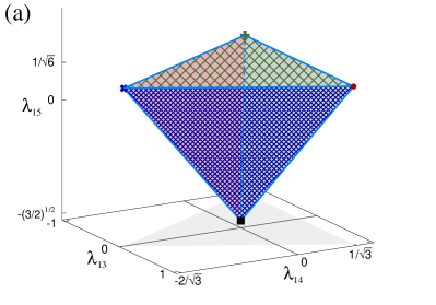
From Eq.(32) where the unit vectors e^jsubscript^𝑒𝑗\hat{e}_{j} are defined to parametrize the probability vector p𝑝\vec{p}, and the relation between the latter and the diagonal Gell-Mann matrices 𝚲jksubscript𝚲𝑗𝑘{\bm{\Lambda}}_{jk}, it is clear that any hypersurface t2subscript𝑡2t_{2} constant is mapped to a sphere in the λ𝜆\lambda-space. The affine space of states in the λ𝜆\lambda-space is a tetrahedron which is shown in Figure 7(a), where the vertices correspond to pure states indicated by dot-, plus-, times-, and square-symbols respectively. Under the map these are

p1λ1subscript𝑝1subscript𝜆1\displaystyle\vec{p}_{1}\to\vec{\lambda}_{1} =\displaystyle= (1,13,16);p2λ2=(1,13,16);11316subscript𝑝2subscript𝜆211316\displaystyle\left(1,\,\frac{1}{\sqrt{3}},\,\frac{1}{\sqrt{6}}\right)\,;\quad\vec{p}_{2}\to\vec{\lambda}_{2}=\left(-1,\,\frac{1}{\sqrt{3}},\,\frac{1}{\sqrt{6}}\right)\,;
p3λ3subscript𝑝3subscript𝜆3\displaystyle\vec{p}_{3}\to\vec{\lambda}_{3} =\displaystyle= (0,23,16);p4λ4=(0, 0,32),02316subscript𝑝4subscript𝜆40 032\displaystyle\left(0,\,-\frac{2}{\sqrt{3}},\,\frac{1}{\sqrt{6}}\right)\,;\qquad\vec{p}_{4}\to\vec{\lambda}_{4}=\left(0,\,0,\,-\sqrt{\frac{3}{2}}\right)\,,

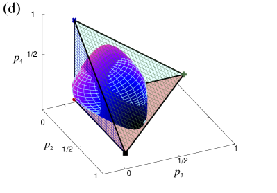
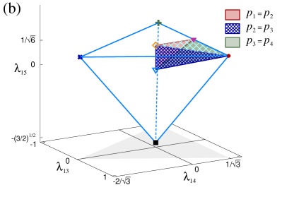
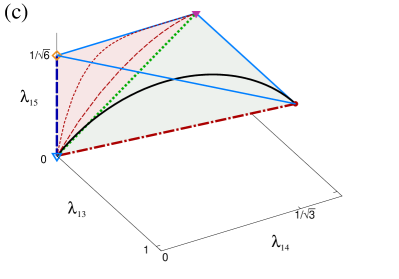
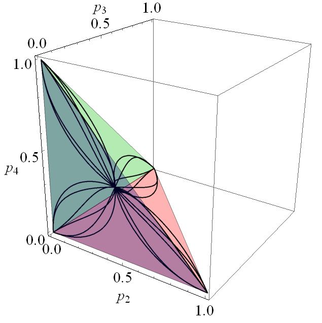
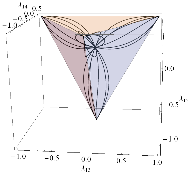
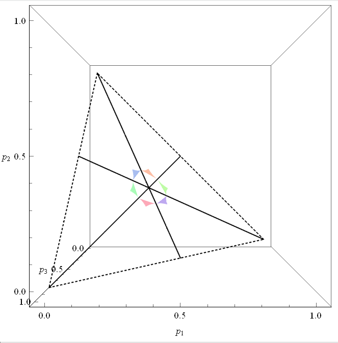
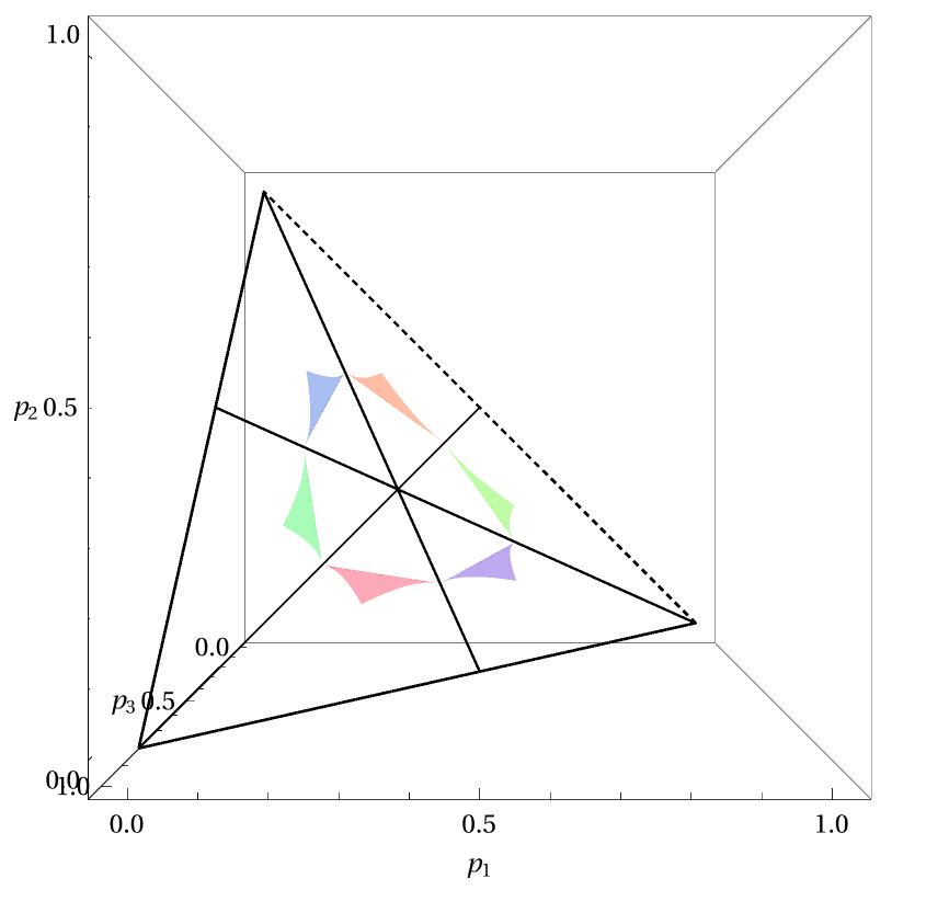
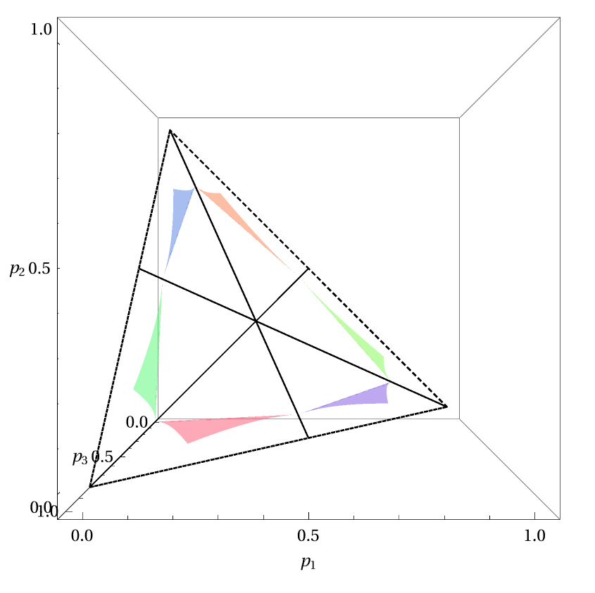
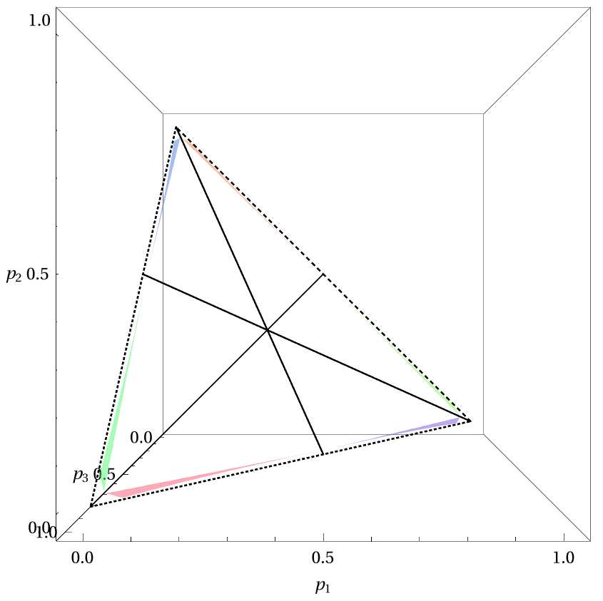
which yield the limit values of λ𝜆\vec{\lambda} for physical states. Referring to this figure, we may visualize the thermal states by assigning a definite meaning to each vertex; thus, we choose p1subscript𝑝1p_{1} to denote the probability of the ground state (dot-symbol), p2subscript𝑝2p_{2} for the probability of the first excited state (plus-symbol), p3subscript𝑝3p_{3} for that of the second excited state (times-symbol), and p4subscript𝑝4p_{4} for that of the third excited state (square-symbol). This would give the condition p1p2p3p4subscript𝑝1subscript𝑝2subscript𝑝3subscript𝑝4p_{1}\geq p_{2}\geq p_{3}\geq p_{4}. The planes defined by p1=p2subscript𝑝1subscript𝑝2p_{1}=p_{2}, p2=p3subscript𝑝2subscript𝑝3p_{2}=p_{3} and p3=p4subscript𝑝3subscript𝑝4p_{3}=p_{4} are mapped onto planes in the λ𝜆\lambda-space and the intersection with the affine space of states provides the faces of the thermal region shown in Fig. 7(b). In this sense, with the exception of the upper face, each point in this region is related to a density matrix of the form Eq. (7). As mentioned before, for infinite temperature the thermal state corresponds to the most mixed state, indicated by an empty triangle-symbol, and for zero temperature the thermal state corresponds to a ground state (dot-symbol) without degeneracy; the case for the ground state with degeneracy is indicated by a triangle-symbol (degeneracy of order two) and empty square-symbol (degeneracy of order three), respectively. So, the thermal state as a function of the temperature moves along a trajectory which connects the most mixed state with one of the other three end points depending of the degeneracy of the system. Fig. 7(c) shows these paths: a solid black line for the general case without degeneracy, while for the degenerate cases the path lies on a face or edge of the affine space; for example, for values p1=p2subscript𝑝1subscript𝑝2p_{1}=p_{2} with p3p1subscript𝑝3subscript𝑝1p_{3}\neq p_{1} and p3p4subscript𝑝3subscript𝑝4p_{3}\neq p_{4} the trajectory is over the face λ13=0subscript𝜆130\lambda_{13}=0 (drawn with a dashed-line for p3p4subscript𝑝3subscript𝑝4p_{3}\approx p_{4}, and with a short-dashed-line for p3p1subscript𝑝3subscript𝑝1p_{3}\approx p_{1}). A similar behavior is had on the other thermal faces defined by the degeneracy p2=p3subscript𝑝2subscript𝑝3p_{2}=p_{3} and p3=p4subscript𝑝3subscript𝑝4p_{3}=p_{4}, with the trajectories on the edges corresponding to the cases for double degeneracy p1=p2subscript𝑝1subscript𝑝2p_{1}=p_{2} and p3=p4subscript𝑝3subscript𝑝4p_{3}=p_{4} (dotted-line), degeneracy of order three p1=p2=p3subscript𝑝1subscript𝑝2subscript𝑝3p_{1}=p_{2}=p_{3} (dashed-line), and when p2=p3=p4subscript𝑝2subscript𝑝3subscript𝑝4p_{2}=p_{3}=p_{4} (dash-dot-line).

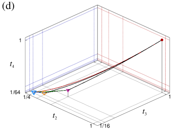
Finally, for λ=r(cos(ϕ)sin(θ),sin(ϕ)sin(θ),cos(θ))𝜆𝑟italic-ϕ𝜃italic-ϕ𝜃𝜃\vec{\lambda}=r\left(\cos(\phi)\sin(\theta),\,\sin(\phi)\sin(\theta),\,\cos(\theta)\right) in spherical coordinates, the non-linear map from λ𝜆\lambda-space to the invariants t𝑡t-space λt=(t2,t3,t4)𝜆𝑡subscript𝑡2subscript𝑡3subscript𝑡4\vec{\lambda}\to\vec{t}=(t_{2},\,t_{3},\,t_{4}) gives us the values tjsubscript𝑡𝑗t_{j} shown by Eq. (33). The end points of the thermal region are mapped to the vertices of the physical region in the t𝑡t-space [cf. Eq. (24)], i.e., these points are representative of a particular kind of states in t𝑡t-space. In the λ𝜆\lambda-space these points are given by λp=(1, 1/3, 1/6)subscript𝜆𝑝11316\vec{\lambda}_{p}=(1,\,1/\sqrt{3},\,1/\sqrt{6}) (ground state), λ12=(0, 1/3, 1/6)subscript𝜆1201316\vec{\lambda}_{12}=(0,\,1/\sqrt{3},\,1/\sqrt{6}) (the degenerate case p1=p2subscript𝑝1subscript𝑝2p_{1}=p_{2}), λ123=(0, 0, 1/6)subscript𝜆1230 016\vec{\lambda}_{123}=(0,\,0,\,1/\sqrt{6}) (the degenerate case p1=p2=p3subscript𝑝1subscript𝑝2subscript𝑝3p_{1}=p_{2}=p_{3}) and λe=(0, 0, 0)subscript𝜆𝑒0 0 0\vec{\lambda}_{e}=(0,\,0,\,0) (the most entangled state), and these are mapped to λpt1subscript𝜆𝑝subscript𝑡1\vec{\lambda}_{p}\to\vec{t}_{1}, λ12t2subscript𝜆12subscript𝑡2\vec{\lambda}_{12}\to\vec{t}_{2}, λ123t3subscript𝜆123subscript𝑡3\vec{\lambda}_{123}\to\vec{t}_{3} and λet4subscript𝜆𝑒subscript𝑡4\vec{\lambda}_{e}\to\vec{t}_{4}; these points together with the boundary of the thermal state region are shown in Fig. 7(d).
Refer to caption
Refer to caption
Refer to caption
Refer to caption
Figure 7: (a) Simplex for a ququart system in the λ𝜆\lambda-space. (b) Thermal state region by choosing the vertices to represent probabilities for for ground state (dot-symbol), first excited state (plus-symbol), second excited state (times-symbol) and third excited state (square-symbol). Other points indicated are for the most entangled state (empty triangle-symbol), the end point for degeneracy p1=p2subscript𝑝1subscript𝑝2p_{1}=p_{2} (solid triangle-symbol) and the end point for degeneracy p1=p2=p3subscript𝑝1subscript𝑝2subscript𝑝3p_{1}=p_{2}=p_{3} (empty square-symbol). (c) Zoom-in of the thermal states region with some trajectories as functions of the temperature. (d) The physical states region in t𝑡t-space obtained from the non-linear map applied to the thermal region in λ𝜆\lambda-space. See text for details.

4 Thermal states

The different diagonal representations discussed above allow us to study several processes related to three– and four–level systems. For example, one may study the thermodynamics of the Gibbs states represented by Eq. (7) for different Hamiltonians. In this section, we present the study for two cases: where the Hamiltonian is given as a linear form of the angular momentum generators 𝑱xsubscript𝑱𝑥{\bm{J}}_{x}, 𝑱ysubscript𝑱𝑦{\bm{J}}_{y}, and 𝑱zsubscript𝑱𝑧{\bm{J}}_{z}; and in the quadratic form described by the LMG Hamiltonian model.

4.1 Linear Hamiltonian

The linear Hamiltonian can be written as

H=ωn^𝑱,𝐻𝜔^𝑛𝑱H=\omega\ \hat{n}\cdot{\bm{J}}\,, (36)

where n^=(sinθcosϕ,sinθsinϕ,cosθ)^𝑛𝜃italic-ϕ𝜃italic-ϕ𝜃\hat{n}={(\sin\theta\cos\phi,\sin\theta\sin\phi,\cos\theta)} denotes the unit vector in spherical coordinates. By means of the basis states of 𝑱2superscript𝑱2{\bm{J}}^{2} and 𝑱nsubscript𝑱𝑛{\bm{J}}_{n} denoted by |J,Mnsubscriptket𝐽𝑀𝑛|J,M\rangle_{n} the eigenvectors and eigenvalues are given by the expressions (=1Planck-constant-over-2-pi1\hbar=1)

EM=ωM;|J,Mn=μ=JJDμ,MJ(0,θ,ϕ)|J,μ,formulae-sequencesubscript𝐸𝑀𝜔𝑀subscriptket𝐽𝑀𝑛subscriptsuperscript𝐽𝜇𝐽subscriptsuperscript𝐷𝐽𝜇𝑀0𝜃italic-ϕket𝐽𝜇E_{M}=\omega\,M\ ;\quad|J,M\rangle_{n}=\sum^{J}_{\mu=-J}D^{J}_{\mu,M}(0,-\theta,\phi)|J,\,\mu\rangle\,, (37)

with M=J,J+1,J1,J𝑀𝐽𝐽1𝐽1𝐽M=-J,-J+1,\cdots J-1,J, and Dμ,MJsubscriptsuperscript𝐷𝐽𝜇𝑀D^{J}_{\mu,M} indicating the Wigner rotational matrix.

For this system, the PME of an ensemble of particles of spin 𝑱𝑱{\bm{J}} and with a well defined mean value of the energy yields a density matrix of the form (cf. Section 2)

ρ=Diag(p1,p2,,p2J,p2J+1),𝜌Diagsubscript𝑝1subscript𝑝2subscript𝑝2𝐽subscript𝑝2𝐽1\rho={\rm Diag}\,\left(p_{1},p_{2},\cdots,p_{2J},p_{2J+1}\right)\,, (38)

with

pM=eβEMM=JJeβEM.subscript𝑝𝑀superscript𝑒𝛽subscript𝐸𝑀subscriptsuperscript𝐽𝑀𝐽superscript𝑒𝛽subscript𝐸𝑀p_{M}=\frac{e^{-\beta\,E_{M}}}{\sum^{J}_{M=-J}e^{-\beta\,E_{M}}}\,. (39)

The expressions (38) and (39) will be used to describe the thermal state of a qutrit with J=1𝐽1J=1 and that of a ququart with J=3/2𝐽32J=3/2. The qutrit corresponding to a 3-level system has equidistant energy levels E1=ωsubscript𝐸1𝜔E_{1}=-\,\omega, E2=0subscript𝐸20E_{2}=0 and E3=ωsubscript𝐸3𝜔E_{3}=\,\omega, and occupation probabilities

p1subscript𝑝1\displaystyle p_{1} =\displaystyle= eβω1+2cosh(βω),p2=11+2cosh(βω),p3=eβω1+2cosh(βω).formulae-sequencesuperscript𝑒𝛽𝜔12𝛽𝜔subscript𝑝2112𝛽𝜔subscript𝑝3superscript𝑒𝛽𝜔12𝛽𝜔\displaystyle\frac{e^{-\beta\,\,\omega}}{1+2\cosh{(\beta\,\,\omega)}}\,,\quad p_{2}=\frac{1}{1+2\cosh{(\beta\,\,\omega)}}\,,\quad p_{3}=\frac{e^{\beta\,\,\omega}}{1+2\cosh{(\beta\,\,\omega)}}\,. (40)

Notice that one gets the same results by considering the matrix Hamiltonian in the basis states of 𝑱2superscript𝑱2{\bm{J}}^{2} and 𝑱zsubscript𝑱𝑧{\bm{J}}_{z}, where its matrix elements depend on the spherical angles (θ,ϕ)𝜃italic-ϕ(\theta,\phi). After the construction of the Boltzmann density matrix is done, its eigenvalues will of course correspond to the occupation probabilities given above.

In the vicinity of the most mixed state (βω𝛽𝜔\beta\,\omega small) the occupation probabilities of the Boltzmann distribution are linear functions of the energy, i.e.,

p113(1βω),p213,p313(1+βω).formulae-sequencesubscript𝑝1131𝛽𝜔formulae-sequencesubscript𝑝213subscript𝑝3131𝛽𝜔p_{1}\approx\frac{1}{3}(1-\beta\,\,\omega)\,,\quad p_{2}\approx\frac{1}{3}\,,\quad p_{3}\approx\frac{1}{3}(1+\beta\,\,\omega)\,. (41)

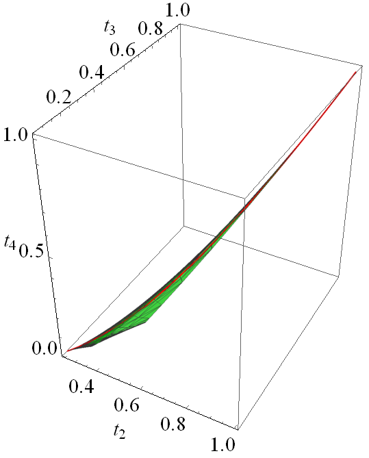
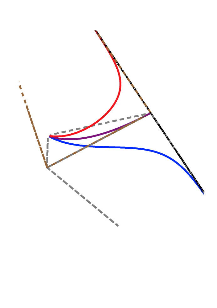
The dependency between the variables t2subscript𝑡2t_{2} and t3subscript𝑡3t_{3} can be seen in Figure 8 (left). The curve defined by the thermal states crosses the allowed region to define a valid quantum system, from the most mixed state (t2=1/3subscript𝑡213t_{2}=1/3, t3=1/9subscript𝑡319t_{3}=1/9) to the pure state state (t2=t3=1subscript𝑡2subscript𝑡31t_{2}=t_{3}=1), which are reached when the temperature of the system is T𝑇T\rightarrow\infty and T0𝑇0T\rightarrow 0, respectively (as mentioned above).

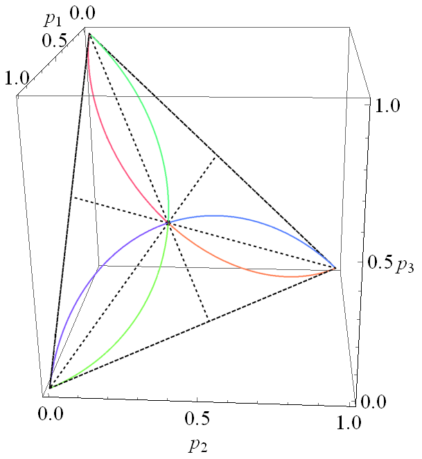
The occupation probabilities (40) satisfy

p22=p1p3,superscriptsubscript𝑝22subscript𝑝1subscript𝑝3p_{2}^{2}=p_{1}\,p_{3}, (42)

and the invariants of the density matrix take the form

t1=1,t2=2cosh(βω)11+2cosh(βω),t3=1+2cosh(3βω)(1+2cosh(βω))3;formulae-sequencesubscript𝑡11formulae-sequencesubscript𝑡22𝛽𝜔112𝛽𝜔subscript𝑡3123𝛽𝜔superscript12𝛽𝜔3t_{1}=1\,,\qquad t_{2}=\frac{2\cosh{(\beta\,\,\omega)}-1}{1+2\cosh({\beta\,\,\omega})}\,,\qquad t_{3}=\frac{1+2\cosh{(3\,\beta\,\,\omega)}}{(1+2\cosh{(\beta\,\,\omega)})^{3}}\,; (43)

they are not independent, as

t3=18(9t223t23+3t2t1),subscript𝑡3189subscriptsuperscript𝑡223subscriptsuperscript𝑡323subscript𝑡2subscript𝑡1t_{3}=\frac{1}{8}\,(9\,t^{2}_{2}-3\,t^{3}_{2}+3\,t_{2}-t_{1})\ , (44)

shown by the interior (red) curve in Figure 8 (left).

Since the labeling of the energy levels of the system is arbitrary, we may take all their possible permutations arriving at the three possible curves

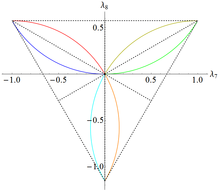
p12=p2p3,p22=p1p3,p32=p1p2.formulae-sequencesuperscriptsubscript𝑝12subscript𝑝2subscript𝑝3formulae-sequencesuperscriptsubscript𝑝22subscript𝑝1subscript𝑝3superscriptsubscript𝑝32subscript𝑝1subscript𝑝2p_{1}^{2}=p_{2}\,p_{3},\quad p_{2}^{2}=p_{1}\,p_{3},\quad p_{3}^{2}=p_{1}\,p_{2}. (45)

These curves follow a three-petal-flower-like structure as shown in Figure 8 (right).

The probabilities allow us to obtain the Gell-Mann parameters

λ7=1eβω1+2cosh(βω),λ8=13sinh(βω)cosh(βω)3(1+2cosh(βω)).formulae-sequencesubscript𝜆71superscript𝑒𝛽𝜔12𝛽𝜔subscript𝜆813𝛽𝜔𝛽𝜔312𝛽𝜔\lambda_{7}=\frac{1-e^{-\beta\,\omega}}{1+2\cosh\left(\beta\,\omega\right)},\quad\lambda_{8}=\frac{1-3\sinh\left(\beta\,\omega\right)-\cosh\left(\beta\,\omega\right)}{\sqrt{3}\,(1+2\cosh\left(\beta\,\omega\right))}. (46)

By using the expressions in Eq. (45) together with (46) and the relation between the λ𝜆\lambda parameters and the probabilities p1=λ72+λ823+13subscript𝑝1subscript𝜆72subscript𝜆82313p_{1}=\frac{\lambda_{7}}{2}+\frac{\lambda_{8}}{2\sqrt{3}}+\frac{1}{3}, p2=λ72+λ823+13subscript𝑝2subscript𝜆72subscript𝜆82313p_{2}=-\frac{\lambda_{7}}{2}+\frac{\lambda_{8}}{2\sqrt{3}}+\frac{1}{3}, and p3=13λ83subscript𝑝313subscript𝜆83p_{3}=\frac{1}{3}-\frac{\lambda_{8}}{\sqrt{3}} one arrives at the following curves in λ𝜆\lambda-space

3λ7(λ7±2)+λ8(3λ8+23)=0,3λ72+λ8(3λ843)=0.formulae-sequence3subscript𝜆7plus-or-minussubscript𝜆72subscript𝜆83subscript𝜆82303superscriptsubscript𝜆72subscript𝜆83subscript𝜆84303\lambda_{7}(\lambda_{7}\pm 2)+\lambda_{8}\left(3\lambda_{8}+2\sqrt{3}\right)=0,\quad 3\lambda_{7}^{2}+\lambda_{8}\left(3\lambda_{8}-4\sqrt{3}\right)=0\ . (47)

The curves follow the same flower-like structure as in the case of the probabilities [see Figure 8 (bottom)].
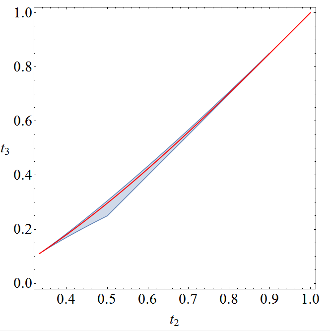
Refer to caption
Refer to caption
Refer to caption
Figure 8: Left: curve defined by the thermal states of a qutrit crossing the allowed physical region which defines a valid quantum system, from the most mixed state (t2=1/3subscript𝑡213t_{2}=1/3, t3=1/9subscript𝑡319t_{3}=1/9) (T𝑇T\rightarrow\infty) to the pure state state (t2=t3=1subscript𝑡2subscript𝑡31t_{2}=t_{3}=1) (T0𝑇0T\rightarrow 0). Right: the same curve defined by the thermal states as seen in p𝑝p-space follows a three-petal-flower-like structure. Bottom: The same flower-like structure is seen in λ𝜆\lambda-space.

4.2 Ququart

For the four-level system the thermal state is given by the following density matrix

𝝆=(f3sinh(η2)csch(2η)34f2ntanh(η2)sech(η)3fn2sinh3(η2)csch(2η)n3sinh4(η2)csch(2η)34f2n+tanh(η2)sech(η)18fgsech(η2)18g+ntanh(η2)3f+n2sinh3(η2)csch(2η)3fn+2sinh3(η2)csch(2η)18g+n+tanh(η2)18f+gsech(η2)34f+2ntanh(η2)sech(η)n+3sinh4(η2)csch(2η)3f+n+2sinh3(η2)csch(2η)34f+2n+tanh(η2)sech(η)f+3sinh(η2)csch(2η))𝝆superscriptsubscript𝑓3𝜂2csch2𝜂34superscriptsubscript𝑓2subscript𝑛𝜂2sech𝜂3subscript𝑓superscriptsubscript𝑛2superscript3𝜂2csch2𝜂superscriptsubscript𝑛3superscript4𝜂2csch2𝜂34superscriptsubscript𝑓2subscript𝑛𝜂2sech𝜂18subscript𝑓subscript𝑔sech𝜂218subscript𝑔subscript𝑛𝜂23subscript𝑓superscriptsubscript𝑛2superscript3𝜂2csch2𝜂3subscript𝑓superscriptsubscript𝑛2superscript3𝜂2csch2𝜂18subscript𝑔subscript𝑛𝜂218subscript𝑓subscript𝑔sech𝜂234superscriptsubscript𝑓2subscript𝑛𝜂2sech𝜂superscriptsubscript𝑛3superscript4𝜂2csch2𝜂3subscript𝑓superscriptsubscript𝑛2superscript3𝜂2csch2𝜂34superscriptsubscript𝑓2subscript𝑛𝜂2sech𝜂superscriptsubscript𝑓3𝜂2csch2𝜂{\bm{\rho}}=\left(\begin{array}[]{cccc}f_{-}^{3}\sinh\left(\frac{\eta}{2}\right){\rm csch}(2\eta)&-\frac{\sqrt{3}}{4}f_{-}^{2}n_{-}\tanh\left(\frac{\eta}{2}\right){\rm sech}(\eta)&\sqrt{3}f_{-}n_{-}^{2}\sinh^{3}\left(\frac{\eta}{2}\right){\rm csch}(2\eta)&-n_{-}^{3}\sinh^{4}\left(\frac{\eta}{2}\right){\rm csch}(2\eta)\\ -\frac{\sqrt{3}}{4}f_{-}^{2}n_{+}\tanh\left(\frac{\eta}{2}\right){\rm sech}(\eta)&\frac{1}{8}f_{-}g_{-}{\rm sech}\left(\frac{\eta}{2}\right)&-\frac{1}{8}g_{+}n_{-}\tanh\left(\frac{\eta}{2}\right)&\sqrt{3}f_{+}n_{-}^{2}\sinh^{3}\left(\frac{\eta}{2}\right){\rm csch}(2\eta)\\ \sqrt{3}f_{-}n_{+}^{2}\sinh^{3}\left(\frac{\eta}{2}\right){\rm csch}(2\eta)&-\frac{1}{8}g_{+}n_{+}\tanh\left(\frac{\eta}{2}\right)&\frac{1}{8}f_{+}g_{-}{\rm sech}\left(\frac{\eta}{2}\right)&-\frac{\sqrt{3}}{4}f_{+}^{2}n_{-}\tanh\left(\frac{\eta}{2}\right){\rm sech}(\eta)\\ -n_{+}^{3}\sinh^{4}\left(\frac{\eta}{2}\right){\rm csch}(2\eta)&\sqrt{3}f_{+}n_{+}^{2}\sinh^{3}\left(\frac{\eta}{2}\right){\rm csch}(2\eta)&-\frac{\sqrt{3}}{4}f_{+}^{2}n_{+}\tanh\left(\frac{\eta}{2}\right){\rm sech}(\eta)&f_{+}^{3}\sinh\left(\frac{\eta}{2}\right){\rm csch}(2\eta)\\ \end{array}\right) (48)

where η=βω𝜂𝛽𝜔\eta=\beta\,\omega, n±=nx±inysubscript𝑛plus-or-minusplus-or-minussubscript𝑛𝑥𝑖subscript𝑛𝑦n_{\pm}=n_{x}\pm in_{y}, f±=cosh(η2)±cos(θ)sinh(η2)subscript𝑓plus-or-minusplus-or-minus𝜂2𝜃𝜂2f_{\pm}=\cosh\left(\frac{\eta}{2}\right)\pm\cos(\theta)\sinh\left(\frac{\eta}{2}\right), g±=3sin2(θ)+(3cos2(θ)±1)sech(η)subscript𝑔plus-or-minus3superscript2𝜃plus-or-minus3superscript2𝜃1sech𝜂g_{\pm}=3\sin^{2}(\theta)+\left(3\cos^{2}(\theta)\pm 1\right){\rm sech}(\eta). Associated to this thermal state the invariants t2subscript𝑡2t_{2}, t3subscript𝑡3t_{3}, and t4subscript𝑡4t_{4}, are equal to

t2=14(4sech2(βω2)2sech(βω)),subscript𝑡2144superscriptsech2𝛽𝜔22sech𝛽𝜔\displaystyle t_{2}=\frac{1}{4}\left(4-{\rm sech}^{2}\left(\frac{\beta\,\omega}{2}\right)-2\,{\rm sech}\left(\beta\,\omega\right)\right),
t3=138(cosh(βω)+1)+3sech(βω)8(sech(βω)3),subscript𝑡3138𝛽𝜔13sech𝛽𝜔8sech𝛽𝜔3\displaystyle t_{3}=1-\frac{3}{8(\cosh\left(\beta\,\omega\right)+1)}+\frac{3\,{\rm sech}\left(\beta\,\omega\right)}{8}\left({\rm sech}\left(\beta\,\omega\right)-3\right),
t4=1128(cosh(2βω)+cosh(6βω))sech4(βω2)sech4(βω).subscript𝑡411282𝛽𝜔6𝛽𝜔superscriptsech4𝛽𝜔2superscriptsech4𝛽𝜔\displaystyle t_{4}=\frac{1}{128}\left(\cosh\left(2\beta\,\omega\right)+\cosh\left(6\beta\,\omega\right)\right){\rm sech}^{4}\left(\frac{\beta\,\omega}{2}\right){\rm sech}^{4}\left(\beta\,\omega\right). (49)

The probabilities can be expressed as follows

p1subscript𝑝1\displaystyle p_{1} =\displaystyle= sinh(3ωβ2)+cosh(3ωβ2)2(cosh(ωβ2)+cosh(3ωβ2)),p2=(tanh(ωβ2)+1)sech2(ωβ2)4(tanh2(ωβ2)+1),3𝜔𝛽23𝜔𝛽22𝜔𝛽23𝜔𝛽2subscript𝑝2𝜔𝛽21superscriptsech2𝜔𝛽24superscript2𝜔𝛽21\displaystyle\frac{\sinh\left(\frac{3\omega\,\beta}{2}\right)+\cosh\left(\frac{3\omega\,\beta}{2}\right)}{2\left(\cosh\left(\frac{\omega\,\beta}{2}\right)+\cosh\left(\frac{3\omega\,\beta}{2}\right)\right)},\qquad\phantom{mmmm}p_{2}=\frac{\left(\tanh\left(\frac{\,\omega\,\beta}{2}\right)+1\right){\rm sech}^{2}\left(\frac{\omega\,\beta}{2}\right)}{4\left(\tanh^{2}\left(\frac{\omega\,\beta}{2}\right)+1\right)},
p3subscript𝑝3\displaystyle p_{3} =\displaystyle= sech4(ωβ2)4(tanh(ωβ2)+1)(tanh2(ωβ2)+1),p4=sech6(ωβ2)4(tanh(ωβ2)+1)3(tanh2(ωβ2)+1),superscriptsech4𝜔𝛽24𝜔𝛽21superscript2𝜔𝛽21subscript𝑝4superscriptsech6𝜔𝛽24superscript𝜔𝛽213superscript2𝜔𝛽21\displaystyle\frac{{\rm sech}^{4}\left(\frac{\omega\,\beta}{2}\right)}{4\left(\tanh\left(\frac{\omega\,\beta}{2}\right)+1\right)\left(\tanh^{2}\left(\frac{\omega\,\beta}{2}\right)+1\right)},\qquad p_{4}=\frac{{\rm sech}^{6}\left(\frac{\omega\,\beta}{2}\right)}{4\left(\tanh\left(\frac{\omega\,\beta}{2}\right)+1\right)^{3}\left(\tanh^{2}\left(\frac{\omega\,\beta}{2}\right)+1\right)},

which in this case have the following explicit correlation

p1p4=p2p3,withp1+p2+p3+p4=1.formulae-sequencesubscript𝑝1subscript𝑝4subscript𝑝2subscript𝑝3withsubscript𝑝1subscript𝑝2subscript𝑝3subscript𝑝41p_{1}\,p_{4}=p_{2}\,p_{3},\quad{\rm with}\quad p_{1}+p_{2}+p_{3}+p_{4}=1. (50)

By taking all the possible permutations of the probabilities we obtain 24 different curves, abbreviated in the following expression

pjpk=plpm,with(j,k,l,m)=𝝅(1,2,3,4),𝝅𝒮4.formulae-sequencesubscript𝑝𝑗subscript𝑝𝑘subscript𝑝𝑙subscript𝑝𝑚withformulae-sequence𝑗𝑘𝑙𝑚𝝅1234𝝅subscript𝒮4p_{j}\,p_{k}=p_{l}\,p_{m},\quad{\rm with}\quad(j,k,l,m)={\bm{\pi}}(1,2,3,4)\,,\quad{\bm{\pi}}\in{\cal S}_{4}\ . (51)

The probabilities of Eq. (4.2) lead us to the Gell-Mann parameters (λ13subscript𝜆13\lambda_{13}, λ14subscript𝜆14\lambda_{14}, λ15subscript𝜆15\lambda_{15}) which take the form

λ13=12tanh(ωβ2)(tanh(ωβ)+1),λ14=(tanh(ωβ2)+1)(3tanh(ωβ)+sech(ωβ)1)43,formulae-sequencesubscript𝜆1312𝜔𝛽2𝜔𝛽1subscript𝜆14𝜔𝛽213𝜔𝛽sech𝜔𝛽143\displaystyle\lambda_{13}=\frac{1}{2}\tanh\left(\frac{\omega\,\beta}{2}\right)(\tanh(\omega\,\beta)+1),\hskip 5.69046pt\lambda_{14}=\frac{\left(\tanh\left(\frac{\omega\,\beta}{2}\right)+1\right)(3\tanh(\omega\,\beta)+{\rm sech}(\omega\,\beta)-1)}{4\sqrt{3}},
λ15=tanh(ωβ2)+tanh(ωβ)+sech(ωβ)16.subscript𝜆15𝜔𝛽2𝜔𝛽sech𝜔𝛽16\displaystyle\lambda_{15}=\frac{\tanh\left(\frac{\omega\,\beta}{2}\right)+\tanh(\omega\,\beta)+{\rm sech}(\omega\,\beta)-1}{\sqrt{6}}. (52)

There are 24 different permutations for the labeling of the states, which define 24 different curves in λ𝜆\lambda-space. One of these satisfies

2λ13(43λ14+56λ156)+8λ142+2λ14(2352λ15)7λ15(2λ15+6)=0.2subscript𝜆1343subscript𝜆1456subscript𝜆1568superscriptsubscript𝜆1422subscript𝜆142352subscript𝜆157subscript𝜆152subscript𝜆1560-2\lambda_{13}\left(4\sqrt{3}\lambda_{14}+5\sqrt{6}\lambda_{15}-6\right)+8\lambda_{14}^{2}+2\lambda_{14}\left(2\sqrt{3}-5\sqrt{2}\lambda_{15}\right)-7\lambda_{15}\left(2\lambda_{15}+\sqrt{6}\right)=0. (53)

which gives us a path in λ𝜆\lambda-space. All such paths can be seen in Figure 9 (each petal consists of 666 of them).

Refer to caption
Refer to caption
Refer to caption
Figure 9: Left: curve defined by the thermal equilibrium states of a ququart crossing the allowed physical region which defines a valid quantum system, from the most mixed state (t2=1/4subscript𝑡214t_{2}=1/4, t3=1/16subscript𝑡3116t_{3}=1/16, t4=1/64subscript𝑡4164t_{4}=1/64) (T𝑇T\rightarrow\infty) to the pure state state (t2=t3=t4=1subscript𝑡2subscript𝑡3subscript𝑡41t_{2}=t_{3}=t_{4}=1) (T0𝑇0T\rightarrow 0). Center: the same curve defined by the thermal states as seen in p𝑝p-space follows a three-petal-flower-like structure; all permutations of the labeling of the states have been taken. Right: The same flower-like structure is seen in λ𝜆\lambda-space. See text for details.

4.3 Lipkin-Meshkov-Glick model

The Lipkin-Meshkov-Glick (LMG) model is a many body quantum system used in several fields like nuclear physics [41, 42, 43], condensed matter [44, 45, 46] and quantum optics [47], which can be written in terms of collective operators in the angular momentum algebra. The Hamiltonian of this model reads as

𝑯=2ω𝑱z+γx𝑱x2+γy𝑱y2.𝑯2𝜔subscript𝑱𝑧subscript𝛾𝑥subscriptsuperscript𝑱2𝑥subscript𝛾𝑦subscriptsuperscript𝑱2𝑦{\bm{H}}=2\,\omega\,{\bm{J}}_{z}+\gamma_{x}\,{\bm{J}}^{2}_{x}+\gamma_{y}\,{\bm{J}}^{2}_{y}\,. (54)

The basis states can be written as follows

|N,n=(Nn)!N!n!𝑱+n|N,0,ket𝑁𝑛𝑁𝑛𝑁𝑛subscriptsuperscript𝑱𝑛ket𝑁0|N,n\rangle=\sqrt{\frac{(N-n)!}{N!\,n!}}\,{\bm{J}}^{n}_{+}|N,0\rangle\,, (55)

where N=2J𝑁2𝐽N=2\,J denotes the number of particles, with J1𝐽1J\geq 1; we have the quantum number n=J+m𝑛𝐽𝑚n=J+m and 𝑱|N,0=0subscript𝑱ket𝑁00{\bm{J}}_{-}|N,0\rangle=0. The Hamiltonian has a symmetry under rotations by π𝜋\pi radians along the Y𝑌Y axis. Thus the eigenstates have definite parity, and can be written as linear combinations of the form,

|s,e=k=0N/2Ck,es|N,2k,|s,o=k=0(N1)/2Dk,os|N,2k+1,formulae-sequenceket𝑠esubscriptsuperscript𝑁2𝑘0subscriptsuperscript𝐶𝑠𝑘eket𝑁2𝑘ketsuperscript𝑠osubscriptsuperscript𝑁12𝑘0subscriptsuperscript𝐷𝑠𝑘oket𝑁2𝑘1|s,{\rm e}\rangle=\sum^{\lfloor N/2\rfloor}_{k=0}C^{s}_{k,{\rm e}}|N,2k\rangle\,,\quad|s^{\prime},{\rm o}\rangle=\sum^{\lfloor(N-1)/2\rfloor}_{k=0}D^{s}_{k,{\rm o}}|N,2k+1\rangle\,, (56)

where the integers s𝑠s and ssuperscript𝑠s^{\prime} take the values s=1,2,,N+12𝑠12𝑁12s=1,2,\cdots,\lceil\frac{N+1}{2}\rceil and s=1,2,,N+12superscript𝑠12𝑁12s^{\prime}=1,2,\cdots,\lfloor\frac{N+1}{2}\rfloor, respectively. By means of the spin coherent states and the catastrophe theory it is possible to determine the quantum phase diagram for the ground state of the LMG model, in the limit N𝑁N\to\infty. This diagram is determined by the locus of points in the control parameter space

(γx,γy)subscript𝛾𝑥subscript𝛾𝑦\displaystyle(\gamma_{x},\gamma_{y}) =\displaystyle= (0,0)ifγx>1,γy>1,formulae-sequence00ifsubscript𝛾𝑥1subscript𝛾𝑦1\displaystyle(0,0)\hskip 28.45274pt\hbox{if}\quad\gamma_{x}>-1\,,\quad\gamma_{y}>-1\,,
γxsubscript𝛾𝑥\displaystyle\qquad\gamma_{x} =\displaystyle= 1,ifγy1,γy<γx,formulae-sequence1ifsubscript𝛾𝑦1subscript𝛾𝑦subscript𝛾𝑥\displaystyle-1\,,\hskip 28.45274pt\hbox{if}\quad\gamma_{y}\leq-1\,,\quad\gamma_{y}<\gamma_{x}\,,
γysubscript𝛾𝑦\displaystyle\qquad\gamma_{y} =\displaystyle= 1,ifγx1,γy>γx,formulae-sequence1ifsubscript𝛾𝑥1subscript𝛾𝑦subscript𝛾𝑥\displaystyle-1\,,\hskip 28.45274pt\hbox{if}\quad\gamma_{x}\leq-1\,,\quad\gamma_{y}>\gamma_{x}\,,
γysubscript𝛾𝑦\displaystyle\qquad\gamma_{y} =\displaystyle= γx,ifγx1.subscript𝛾𝑥ifsubscript𝛾𝑥1\displaystyle\gamma_{x}\,,\hskip 25.6073pt\quad\hbox{if}\quad\gamma_{x}\leq-1\,. (57)

Notice that the intersection of even and odd energy surfaces yields a Maxwell set γy=1/γxsubscript𝛾𝑦1subscript𝛾𝑥\gamma_{y}=1/\gamma_{x}; in the region between the branches of this hyperbola there is no degeneracy between the energy levels of the LMG model, whereas in the exterior part degeneracy is present. By means of the Ehrenfest classification the order of the quantum phase transitions may be determined. One finds second order transitions when the straight lines γx=1subscript𝛾𝑥1\gamma_{x}=-1, γy=1subscript𝛾𝑦1\gamma_{y}=-1 and γy=γxsubscript𝛾𝑦subscript𝛾𝑥\gamma_{y}=\gamma_{x} are crossed. When the line γy=γxsubscript𝛾𝑦subscript𝛾𝑥\gamma_{y}=\gamma_{x} is traversed, first order transitions are exhibited. Finally if the point (γx,γy)=(1,1)subscript𝛾𝑥subscript𝛾𝑦11(\gamma_{x},\gamma_{y})=(-1,-1) is crossed along the straight line γy=γx2subscript𝛾𝑦subscript𝛾𝑥2\gamma_{y}=-\gamma_{x}-2 a third order transitions is present [48].

Here, we will consider the LMG model for N=2𝑁2N=2 particles (J=1𝐽1J=1), given in units of 2ω2𝜔2\,\omega as

𝑯=𝑱z+gx𝑱x2+gy𝑱y2,𝑯subscript𝑱𝑧subscript𝑔𝑥superscriptsubscript𝑱𝑥2subscript𝑔𝑦superscriptsubscript𝑱𝑦2{\bm{H}}={\bm{J}}_{z}+g_{x}{\bm{J}}_{x}^{2}+g_{y}{\bm{J}}_{y}^{2},

where gx=γx/(2ω)subscript𝑔𝑥subscript𝛾𝑥2𝜔g_{x}=\gamma_{x}/(2\omega) and gy=γy/(2ω)subscript𝑔𝑦subscript𝛾𝑦2𝜔g_{y}=\gamma_{y}/(2\omega). Then thermal states associated to the Hamiltonian for N=2𝑁2N=2 particles are given by the following density matrix,

𝝆=(𝝆o00𝝆e),𝝆o=(12eβg+2cosh(12βg2+4)+1),formulae-sequence𝝆subscript𝝆𝑜00subscript𝝆𝑒subscript𝝆𝑜12superscript𝑒𝛽subscript𝑔212𝛽superscriptsubscript𝑔241{\bm{\rho}}=\left(\begin{array}[]{cc}{\bm{\rho}}_{o}&0\\ 0&{\bm{\rho}}_{e}\end{array}\right)\ ,\quad{\bm{\rho}}_{o}=\left(\frac{1}{2e^{\frac{\beta g_{+}}{2}}\cosh\left(\frac{1}{2}\beta\sqrt{g_{-}^{2}+4}\right)+1}\right)\ ,
𝝆e=(eβg+2(cosh(12βg2+4)2sinh(12βg2+4)g2+4)2eβg+2cosh(12βg2+4)+1geβg+2sinh(12βg2+4)g2+4(2eβg+2cosh(12βg2+4)+1)geβg+2sinh(12βg2+4)g2+4(2eβg+2cosh(12βg2+4)+1)eβg+2(2sinh(12βg2+4)g2+4+cosh(12βg2+4))2eβg+2cosh(12βg2+4)+1),subscript𝝆𝑒superscript𝑒𝛽subscript𝑔212𝛽superscriptsubscript𝑔24212𝛽superscriptsubscript𝑔24superscriptsubscript𝑔242superscript𝑒𝛽subscript𝑔212𝛽superscriptsubscript𝑔241subscript𝑔superscript𝑒𝛽subscript𝑔212𝛽superscriptsubscript𝑔24superscriptsubscript𝑔242superscript𝑒𝛽subscript𝑔212𝛽superscriptsubscript𝑔241subscript𝑔superscript𝑒𝛽subscript𝑔212𝛽superscriptsubscript𝑔24superscriptsubscript𝑔242superscript𝑒𝛽subscript𝑔212𝛽superscriptsubscript𝑔241superscript𝑒𝛽subscript𝑔2212𝛽superscriptsubscript𝑔24superscriptsubscript𝑔2412𝛽superscriptsubscript𝑔242superscript𝑒𝛽subscript𝑔212𝛽superscriptsubscript𝑔241{\bm{\rho}}_{e}=\left(\begin{array}[]{cc}\frac{e^{\frac{\beta g_{+}}{2}}\left(\cosh\left(\frac{1}{2}\beta\sqrt{g_{-}^{2}+4}\right)-\frac{2\sinh\left(\frac{1}{2}\beta\sqrt{g_{-}^{2}+4}\right)}{\sqrt{g_{-}^{2}+4}}\right)}{2e^{\frac{\beta g_{+}}{2}}\cosh\left(\frac{1}{2}\beta\sqrt{g_{-}^{2}+4}\right)+1}&-\frac{g_{-}e^{\frac{\beta g_{+}}{2}}\sinh\left(\frac{1}{2}\beta\sqrt{g_{-}^{2}+4}\right)}{\sqrt{g_{-}^{2}+4}\left(2e^{\frac{\beta g_{+}}{2}}\cosh\left(\frac{1}{2}\beta\sqrt{g_{-}^{2}+4}\right)+1\right)}\\[28.45274pt] -\frac{g_{-}e^{\frac{\beta g_{+}}{2}}\sinh\left(\frac{1}{2}\beta\sqrt{g_{-}^{2}+4}\right)}{\sqrt{g_{-}^{2}+4}\left(2e^{\frac{\beta g_{+}}{2}}\cosh\left(\frac{1}{2}\beta\sqrt{g_{-}^{2}+4}\right)+1\right)}&\frac{e^{\frac{\beta g_{+}}{2}}\left(\frac{2\sinh\left(\frac{1}{2}\beta\sqrt{g_{-}^{2}+4}\right)}{\sqrt{g_{-}^{2}+4}}+\cosh\left(\frac{1}{2}\beta\sqrt{g_{-}^{2}+4}\right)\right)}{2e^{\frac{\beta g_{+}}{2}}\cosh\left(\frac{1}{2}\beta\sqrt{g_{-}^{2}+4}\right)+1}\end{array}\right)\ , (58)

where 𝝆osubscript𝝆𝑜{\bm{\rho}}_{o} is a 1×1111\times 1 matrix and 𝝆esubscript𝝆𝑒{\bm{\rho}}_{e} is a 2×2222\times 2 matrix, exhibiting the symmetry invariance of the Hamiltonian, since the Hilbert space divides itself into odd and even subspaces as mentioned previously. The eigenvalue of 𝝆osubscript𝝆𝑜{\bm{\rho}}_{o}

ρ11=11+2eβg+2cosh(12βg2+4),subscript𝜌11112superscript𝑒𝛽subscript𝑔212𝛽superscriptsubscript𝑔24\rho_{11}=\frac{1}{1+2e^{\frac{\beta g_{+}}{2}}\cosh\left(\frac{1}{2}\beta\sqrt{g_{-}^{2}+4}\right)}\ ,

is the probability of finding the system in the odd state. For the even subspace 𝝆esubscript𝝆𝑒{\bm{\rho}}_{e} the eigenvalues

ρ22=e12β(g++g2+4)1+2eβg+2cosh(12βg2+4),ρ33=e12β(g+g2+4)1+2eβg+2cosh(12βg2+4),formulae-sequencesubscript𝜌22superscript𝑒12𝛽subscript𝑔superscriptsubscript𝑔2412superscript𝑒𝛽subscript𝑔212𝛽superscriptsubscript𝑔24subscript𝜌33superscript𝑒12𝛽subscript𝑔superscriptsubscript𝑔2412superscript𝑒𝛽subscript𝑔212𝛽superscriptsubscript𝑔24\rho_{22}=\frac{e^{\frac{1}{2}\beta\left(g_{+}+\sqrt{g_{-}^{2}+4}\right)}}{1+2e^{\frac{\beta g_{+}}{2}}\cosh\left(\frac{1}{2}\beta\sqrt{g_{-}^{2}+4}\right)}\ ,\quad\rho_{33}=\frac{e^{\frac{1}{2}\beta\left(g_{+}-\sqrt{g_{-}^{2}+4}\right)}}{1+2e^{\frac{\beta g_{+}}{2}}\cosh\left(\frac{1}{2}\beta\sqrt{g_{-}^{2}+4}\right)}\ ,

stand for the probabilities of the ground and excited states of the system. We have defined g±:=gx±gyassignsubscript𝑔plus-or-minusplus-or-minussubscript𝑔𝑥subscript𝑔𝑦g_{\pm}:=g_{x}\pm g_{y}.

We are here considering an ensemble of two-particles, with definite angular momentum J=1𝐽1J=1, but without a well defined projection along the Z𝑍Z axes.

As the numeration of the eigenvalues of 𝝆𝝆{\bm{\rho}} is arbitrary, the probabilities can be represented by any permutation (p1,p2,p3)=𝝅(ρ11,ρ22,ρ33)subscript𝑝1subscript𝑝2subscript𝑝3𝝅subscript𝜌11subscript𝜌22subscript𝜌33(p_{1},\,p_{2},\,p_{3})={\bm{\pi}}(\rho_{11},\,\rho_{22},\,\rho_{33}). The correlation between them depends exponentially on the temperature and Hamiltonian parameters β(gx+gy)𝛽subscript𝑔𝑥subscript𝑔𝑦\beta(g_{x}+g_{y}) as

p12=eβ(gx+gy)p2p3.superscriptsubscript𝑝12superscript𝑒𝛽subscript𝑔𝑥subscript𝑔𝑦subscript𝑝2subscript𝑝3p_{1}^{2}=e^{\beta(g_{x}+g_{y})}p_{2}\,p_{3}. (59)

The invariants of the density matrix are found to be

t2=1+2eβg+cosh(βg2+4)(1+2eβg+2cosh(12βg2+4))2,t3=1+2e3βg+2cosh(32βg2+4)(1+2eβg+2cosh(12βg2+4))3.formulae-sequencesubscript𝑡212superscript𝑒𝛽subscript𝑔𝛽superscriptsubscript𝑔24superscript12superscript𝑒𝛽subscript𝑔212𝛽superscriptsubscript𝑔242subscript𝑡312superscript𝑒3𝛽subscript𝑔232𝛽superscriptsubscript𝑔24superscript12superscript𝑒𝛽subscript𝑔212𝛽superscriptsubscript𝑔243t_{2}=\frac{1+2e^{\beta g_{+}}\cosh\left(\beta\sqrt{g_{-}^{2}+4}\right)}{\left(1+2e^{\frac{\beta g_{+}}{2}}\cosh\left(\frac{1}{2}\beta\sqrt{g_{-}^{2}+4}\right)\right)^{2}},\quad t_{3}=\frac{1+2e^{\frac{3\beta g_{+}}{2}}\cosh\left(\frac{3}{2}\beta\sqrt{g_{-}^{2}+4}\right)}{\left(1+2e^{\frac{\beta g_{+}}{2}}\cosh\left(\frac{1}{2}\beta\sqrt{g_{-}^{2}+4}\right)\right)^{3}}. (60)

Thus the thermal states can be located anywhere in the 2-simplex defined by the points (p1,p2,p3)subscript𝑝1subscript𝑝2subscript𝑝3(p_{1},p_{2},p_{3}). For example when β0𝛽0\beta\to 0 one gets the most mixed state, while for β𝛽\beta\to\infty the eigenvalues are equal to (p1=0,p2=1,p3=0)formulae-sequencesubscript𝑝10formulae-sequencesubscript𝑝21subscript𝑝30(p_{1}=0,\,p_{2}=1,\,p_{3}=0); and due to the symmetry under the permutation group, all the regions can be reached by a thermal state of the LMG model. Given this, one can study the dependency of the eigenvalues (p1,p2,p3)subscript𝑝1subscript𝑝2subscript𝑝3(p_{1},p_{2},p_{3}), the invariants t2subscript𝑡2t_{2} and t3subscript𝑡3t_{3}, and the Gell-Mann parameters λ7subscript𝜆7\lambda_{7} and λ8subscript𝜆8\lambda_{8} in terms of the temperature and the Hamiltonian parameters.

As one can see in the previous expressions, the system can be defined by the parameters x=βg+𝑥𝛽subscript𝑔x=\beta g_{+} and y=βg2+4𝑦𝛽superscriptsubscript𝑔24y=\beta\sqrt{g_{-}^{2}+4}, which are used to visualize the different properties in a three-dimensional space. Since the energies of the LMG Hamiltonian can be written as E0=g+subscript𝐸0subscript𝑔E_{0}=g_{+}, E±=12(g+±g2+4)subscript𝐸plus-or-minus12plus-or-minussubscript𝑔superscriptsubscript𝑔24E_{\pm}=\frac{1}{2}(g_{+}\pm\sqrt{g_{-}^{2}+4}), we may identify the parameters as x=βE0𝑥𝛽subscript𝐸0x=\beta E_{0} and y=β(E+E)𝑦𝛽subscript𝐸subscript𝐸y=\beta(E_{+}-E_{-}).

In Figure 10 the parametric plots for probabilities p1subscript𝑝1p_{1}, p2subscript𝑝2p_{2}, and p3subscript𝑝3p_{3} for different values of the LMG Hamiltonian parameters gxsubscript𝑔𝑥g_{x} and gysubscript𝑔𝑦g_{y} and for the case of angular momentum equal to one are shown. Each figure is plotted for a fixed temperature and each color corresponds to a different permutation of the three levels of the system. We emphasize that the points of each permutation are located within specific zones of the simplex, and each zone is delimited by a median, a bisector and the outer simplex boundary. The non-crossing of these zones indicates that the values of the probabilities maintain a certain order (for example, p1>p2>p3subscript𝑝1subscript𝑝2subscript𝑝3p_{1}>p_{2}>p_{3}) and there is no zone where this order is different. This is because the median and bisector lines are the points where two probabilities are equal and the allowed zones do no touch them due to the small value of the non-linearity of the system (in this case gx,gy(1,1)subscript𝑔𝑥subscript𝑔𝑦11g_{x},g_{y}\in(-1,1)). Nonetheless, when the values of gxsubscript𝑔𝑥g_{x} and gysubscript𝑔𝑦g_{y} grow larger (and so do the non-linearity) one can have two equal probabilities or any other possibility as one can see in Figure 11, where different crossings between the zones are shown. Specifically, this change of behavior (non-crossing versus crossing) has as a limit the situation where two probabilities are equal, and this takes place when gx=1/gysubscript𝑔𝑥1subscript𝑔𝑦g_{x}=1/g_{y}. Also, in Figures 10 and 11, one can see that for a small temperature (β1much-greater-than𝛽1\beta\gg 1) the system approaches a pure state (the ground state of the Hamiltonian), while for a large temperature (β1much-less-than𝛽1\beta\ll 1) the system approaches the most mixed state where p1=p2=p3=1/3subscript𝑝1subscript𝑝2subscript𝑝313p_{1}=p_{2}=p_{3}=1/3.

Refer to caption
Refer to caption
Refer to caption
Refer to caption
Figure 10: Probabilities for the three-level diagonal thermal equilibrium state defined by the LMG Hamiltonian model for a) β=1/5𝛽15\beta=1/5, b) β=1/2𝛽12\beta=1/2, c) β=1𝛽1\beta=1, and d) β=2𝛽2\beta=2. In all the cases j=1𝑗1j=1 (qutrit) and gx,gy(1, 1)subscript𝑔𝑥subscript𝑔𝑦11g_{x},g_{y}\in(-1,\,1).
Refer to caption
Refer to caption
Refer to caption
Refer to caption
Figure 11: Probabilities for the three-level diagonal thermal equilibrium state defined by the LMG Hamiltonian for a) β=1/20𝛽120\beta=1/20, b) β=1/2𝛽12\beta=1/2, c) β=1𝛽1\beta=1, and d) β=2𝛽2\beta=2. In all the cases j=1𝑗1j=1 (qutrit) and gx,gy[3, 3]subscript𝑔𝑥subscript𝑔𝑦33g_{x},g_{y}\in[-3,\,3].

4.4 Ququart

For the angular momentum j=3/2𝑗32j=3/2 the thermal density matrix for the LMG Hamiltonian model can be written as

𝝆=(𝝆o00𝝆e),𝝆subscript𝝆𝑜00subscript𝝆𝑒{\bm{\rho}}=\left(\begin{array}[]{cc}{\bm{\rho}}_{o}&0\\ 0&{\bm{\rho}}_{e}\end{array}\right)\,, (61)

with

𝝆o=(eβ(x1cosh(βx12)(g++2)sinh(βx12))2x1(eβcosh(βx12)+cosh(βx22))3eβgsinh(βx12)2eβx1cosh(βx12)+2x1cosh(βx22)3eβgsinh(βx12)2eβx1cosh(βx12)+2x1cosh(βx22)eβ((g++2)tanh(βx12)+x1)2x1(eβ+sech(βx12)cosh(βx22))),subscript𝝆𝑜superscript𝑒𝛽subscript𝑥1𝛽subscript𝑥12subscript𝑔2𝛽subscript𝑥122subscript𝑥1superscript𝑒𝛽𝛽subscript𝑥12𝛽subscript𝑥223superscript𝑒𝛽subscript𝑔𝛽subscript𝑥122superscript𝑒𝛽subscript𝑥1𝛽subscript𝑥122subscript𝑥1𝛽subscript𝑥223superscript𝑒𝛽subscript𝑔𝛽subscript𝑥122superscript𝑒𝛽subscript𝑥1𝛽subscript𝑥122subscript𝑥1𝛽subscript𝑥22superscript𝑒𝛽subscript𝑔2𝛽subscript𝑥12subscript𝑥12subscript𝑥1superscript𝑒𝛽sech𝛽subscript𝑥12𝛽subscript𝑥22{\bm{\rho}}_{o}=\left(\begin{array}[]{cc}\frac{e^{\beta}\left(x_{1}\cosh\left(\frac{\beta x_{1}}{2}\right)-(g_{+}+2)\sinh\left(\frac{\beta x_{1}}{2}\right)\right)}{2x_{1}\left(e^{\beta}\cosh\left(\frac{\beta x_{1}}{2}\right)+\cosh\left(\frac{\beta x_{2}}{2}\right)\right)}&-\frac{\sqrt{3}e^{\beta}g_{-}\sinh\left(\frac{\beta x_{1}}{2}\right)}{2e^{\beta}x_{1}\cosh\left(\frac{\beta x_{1}}{2}\right)+2x_{1}\cosh\left(\frac{\beta x_{2}}{2}\right)}\\[28.45274pt] -\frac{\sqrt{3}e^{\beta}g_{-}\sinh\left(\frac{\beta x_{1}}{2}\right)}{2e^{\beta}x_{1}\cosh\left(\frac{\beta x_{1}}{2}\right)+2x_{1}\cosh\left(\frac{\beta x_{2}}{2}\right)}&\frac{e^{\beta}\left((g_{+}+2)\tanh\left(\frac{\beta x_{1}}{2}\right)+x_{1}\right)}{2x_{1}\left(e^{\beta}+{\rm sech}\left(\frac{\beta x_{1}}{2}\right)\cosh\left(\frac{\beta x_{2}}{2}\right)\right)}\end{array}\right)\ ,
𝝆e=((g+2)sinh(βx22)+x2cosh(βx22)2x2(eβcosh(βx12)+cosh(βx22))3gsinh(βx22)2eβx2cosh(βx12)+2x2cosh(βx22)3gsinh(βx22)2eβx2cosh(βx12)+2x2cosh(βx22)x2cosh(βx22)(g+2)sinh(βx22)2x2(eβcosh(βx12)+cosh(βx22))),subscript𝝆𝑒subscript𝑔2𝛽subscript𝑥22subscript𝑥2𝛽subscript𝑥222subscript𝑥2superscript𝑒𝛽𝛽subscript𝑥12𝛽subscript𝑥223subscript𝑔𝛽subscript𝑥222superscript𝑒𝛽subscript𝑥2𝛽subscript𝑥122subscript𝑥2𝛽subscript𝑥22missing-subexpressionmissing-subexpression3subscript𝑔𝛽subscript𝑥222superscript𝑒𝛽subscript𝑥2𝛽subscript𝑥122subscript𝑥2𝛽subscript𝑥22subscript𝑥2𝛽subscript𝑥22subscript𝑔2𝛽subscript𝑥222subscript𝑥2superscript𝑒𝛽𝛽subscript𝑥12𝛽subscript𝑥22missing-subexpressionmissing-subexpression{\bm{\rho}}_{e}=\left(\begin{array}[]{cccc}\frac{(g_{+}-2)\sinh\left(\frac{\beta x_{2}}{2}\right)+x_{2}\cosh\left(\frac{\beta x_{2}}{2}\right)}{2x_{2}\left(e^{\beta}\cosh\left(\frac{\beta x_{1}}{2}\right)+\cosh\left(\frac{\beta x_{2}}{2}\right)\right)}&-\frac{\sqrt{3}g_{-}\sinh\left(\frac{\beta x_{2}}{2}\right)}{2e^{\beta}x_{2}\cosh\left(\frac{\beta x_{1}}{2}\right)+2x_{2}\cosh\left(\frac{\beta x_{2}}{2}\right)}\\[28.45274pt] -\frac{\sqrt{3}g_{-}\sinh\left(\frac{\beta x_{2}}{2}\right)}{2e^{\beta}x_{2}\cosh\left(\frac{\beta x_{1}}{2}\right)+2x_{2}\cosh\left(\frac{\beta x_{2}}{2}\right)}&\frac{x_{2}\cosh\left(\frac{\beta x_{2}}{2}\right)-(g_{+}-2)\sinh\left(\frac{\beta x_{2}}{2}\right)}{2x_{2}\left(e^{\beta}\cosh\left(\frac{\beta x_{1}}{2}\right)+\cosh\left(\frac{\beta x_{2}}{2}\right)\right)}\end{array}\right)\ ,

where x1=(g++2)2+3g2subscript𝑥1superscriptsubscript𝑔223superscriptsubscript𝑔2x_{1}=\sqrt{(g_{+}+2)^{2}+3g_{-}^{2}} and x2=(g+2)2+3g2subscript𝑥2superscriptsubscript𝑔223superscriptsubscript𝑔2x_{2}=\sqrt{(g_{+}-2)^{2}+3g_{-}^{2}}.

The eigenvalues of the system are

p1=eβx222(eβcosh(βx12)+cosh(βx22)),p2=eβx222(eβcosh(βx12)+cosh(βx22)),formulae-sequencesubscript𝑝1superscript𝑒𝛽subscript𝑥222superscript𝑒𝛽𝛽subscript𝑥12𝛽subscript𝑥22subscript𝑝2superscript𝑒𝛽subscript𝑥222superscript𝑒𝛽𝛽subscript𝑥12𝛽subscript𝑥22\displaystyle p_{1}=\frac{e^{\frac{\beta\,x_{2}}{2}}}{2\left(e^{\beta}\,\cosh\left(\frac{\beta\,x_{1}}{2}\right)+\cosh\left(\frac{\beta\,x_{2}}{2}\right)\right)},\quad p_{2}=\frac{e^{-\frac{\beta\,x_{2}}{2}}}{2\left(e^{\beta}\cosh\left(\frac{\beta\,x_{1}}{2}\right)+\cosh\left(\frac{\beta\,x_{2}}{2}\right)\right)},
p3=eβ2(x1+2)2(eβcosh(βx12)+cosh(βx22)),p4=eβ2(x12)2(eβcosh(βx12)+cosh(βx22)).formulae-sequencesubscript𝑝3superscript𝑒𝛽2subscript𝑥122superscript𝑒𝛽𝛽subscript𝑥12𝛽subscript𝑥22subscript𝑝4superscript𝑒𝛽2subscript𝑥122superscript𝑒𝛽𝛽subscript𝑥12𝛽subscript𝑥22\displaystyle p_{3}=\frac{e^{\frac{\beta}{2}\,(x_{1}+2)}}{2\left(e^{\beta}\cosh\left(\frac{\beta\,x_{1}}{2}\right)+\cosh\left(\frac{\beta\,x_{2}}{2}\right)\right)},\quad p_{4}=\frac{e^{-\frac{\beta}{2}\left(x_{1}-2\right)}}{2\left(e^{\beta}\,\cosh\left(\frac{\beta\,x_{1}}{2}\right)+\cosh\left(\frac{\beta\,x_{2}}{2}\right)\right)}. (62)

In this case we have a temperature dependent correlation function as the probabilities satisfy

p1p2=eβp3p4.subscript𝑝1subscript𝑝2superscript𝑒𝛽subscript𝑝3subscript𝑝4p_{1}\,p_{2}=e^{\beta}\,p_{3}\,p_{4}\ . (63)

The invariants t2subscript𝑡2t_{2}, t3subscript𝑡3t_{3}, and t4subscript𝑡4t_{4} can be written as

t2=e2βcosh(βx1)+cosh(βx2)2(eβcosh(βx12)+cosh(βx22))2,t3=e32β(x12)+e32β(x1+2)+e32βx2+e3βx228(eβcosh(βx12)+cosh(βx22))3,formulae-sequencesubscript𝑡2superscript𝑒2𝛽𝛽subscript𝑥1𝛽subscript𝑥22superscriptsuperscript𝑒𝛽𝛽subscript𝑥12𝛽subscript𝑥222subscript𝑡3superscript𝑒32𝛽subscript𝑥12superscript𝑒32𝛽subscript𝑥12superscript𝑒32𝛽subscript𝑥2superscript𝑒3𝛽subscript𝑥228superscriptsuperscript𝑒𝛽𝛽subscript𝑥12𝛽subscript𝑥223\displaystyle t_{2}=\frac{e^{2\,\beta}\,\cosh(\beta\,x_{1})+\cosh(\beta\,x_{2})}{2\left(e^{\beta}\,\cosh\left(\frac{\beta\,x_{1}}{2}\right)+\cosh\left(\frac{\beta\,x_{2}}{2}\right)\right)^{2}},\quad t_{3}=\frac{e^{-\frac{3}{2}\,\beta\,(x_{1}-2)}+e^{\frac{3}{2}\,\beta(x_{1}+2)}+e^{-\frac{3}{2}\,\beta\,x_{2}}+e^{\frac{3\,\beta\,x_{2}}{2}}}{8\left(e^{\beta}\,\cosh\left(\frac{\beta\,x_{1}}{2}\right)+\cosh\left(\frac{\beta\,x_{2}}{2}\right)\right)^{3}},
t4=e2β(x12)+e2β(x1+2)+e2βx2+e2βx216(eβcosh(βx12)+cosh(βx22))4,subscript𝑡4superscript𝑒2𝛽subscript𝑥12superscript𝑒2𝛽subscript𝑥12superscript𝑒2𝛽subscript𝑥2superscript𝑒2𝛽subscript𝑥216superscriptsuperscript𝑒𝛽𝛽subscript𝑥12𝛽subscript𝑥224\displaystyle t_{4}=\frac{e^{-2\,\beta(x_{1}-2)}+e^{2\,\beta\,(x_{1}+2)}+e^{-2\beta x_{2}}+e^{2\,\beta\,x_{2}}}{16\left(e^{\beta}\,\cosh\left(\frac{\beta\,x_{1}}{2}\right)+\cosh\left(\frac{\beta\,x_{2}}{2}\right)\right)^{4}}\,, (64)

while the Gell-Mann parameters λ13subscript𝜆13\lambda_{13}, λ14subscript𝜆14\lambda_{14}, and λ15subscript𝜆15\lambda_{15} take the form

λ13=1eβcosh(βx12)csch(βx22)+coth(βx22),λ14=cosh(βx22)eβ+βx123(eβcosh(βx12)+cosh(βx22)),formulae-sequencesubscript𝜆131superscript𝑒𝛽𝛽subscript𝑥12csch𝛽subscript𝑥22hyperbolic-cotangent𝛽subscript𝑥22subscript𝜆14𝛽subscript𝑥22superscript𝑒𝛽𝛽subscript𝑥123superscript𝑒𝛽𝛽subscript𝑥12𝛽subscript𝑥22\displaystyle\lambda_{13}=\frac{1}{e^{\beta}\,\cosh\left(\frac{\beta\,x_{1}}{2}\right){\rm csch}\left(\frac{\beta\,x_{2}}{2}\right)+\coth\left(\frac{\beta\,x_{2}}{2}\right)},\quad\lambda_{14}=\frac{\cosh\left(\frac{\beta\,x_{2}}{2}\right)-e^{\beta+\frac{\beta\,x_{1}}{2}}}{\sqrt{3}\left(e^{\beta}\,\cosh\left(\frac{\beta\,x_{1}}{2}\right)+\cosh\left(\frac{\beta\,x_{2}}{2}\right)\right)},
λ15=16(4eβeβ+eβ+βx1+2eβx12cosh(βx22)).subscript𝜆15164superscript𝑒𝛽superscript𝑒𝛽superscript𝑒𝛽𝛽subscript𝑥12superscript𝑒𝛽subscript𝑥12𝛽subscript𝑥22\displaystyle\lambda_{15}=-\frac{1}{\sqrt{6}}\left(\frac{4\,e^{\beta}}{e^{\beta}+e^{\beta+\beta x_{1}}+2\,e^{\frac{\beta\,x_{1}}{2}}\cosh\left(\frac{\beta\,x_{2}}{2}\right)}\right). (65)

In the four-level system we have a similar behavior as in the qutrit case. Here the zones where the probabilities follow a certain order (say p1>p2>p3>p4subscript𝑝1subscript𝑝2subscript𝑝3subscript𝑝4p_{1}>p_{2}>p_{3}>p_{4}) are delimited by one of 24 different tetrahedrons inside the 3-simplex of Figure 5. Any crossing between these 24 tetrahedrons means that the intended order is no longer satisfied (for example p1>p2>p3>p4subscript𝑝1subscript𝑝2subscript𝑝3subscript𝑝4p_{1}>p_{2}>p_{3}>p_{4} changes to p2>p1>p3>p4subscript𝑝2subscript𝑝1subscript𝑝3subscript𝑝4p_{2}>p_{1}>p_{3}>p_{4} in two different tetrahedrons).

In the case of the LMG model the different behavior (non-crossing versus crossing of different zones) is given when the values of two probabilities are equal, and this takes place when gx=1/(4gy)subscript𝑔𝑥14subscript𝑔𝑦g_{x}=1/(4g_{y}). Figure 12 shows the parametric plot for three different cases: gx=1/(4gy)subscript𝑔𝑥14subscript𝑔𝑦g_{x}=1/(4g_{y}) (purple line) where the thermal evolution is given along the limit between two regions, gx<1/(4gy)subscript𝑔𝑥14subscript𝑔𝑦g_{x}<1/(4g_{y}) (blue line) where the thermal evolution takes place inside one defined region, and gx>1/(4gy)subscript𝑔𝑥14subscript𝑔𝑦g_{x}>1/(4g_{y}) (red line) where the thermal evolution takes place inside another region.
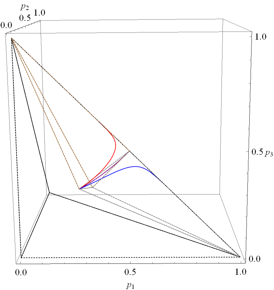
Refer to caption
Refer to caption
Figure 12: Left: Parametric plot for the probabilities p1subscript𝑝1p_{1}, p2subscript𝑝2p_{2}, and p3subscript𝑝3p_{3} for the four-level thermal equilibrium state in the LMG Hamiltonian model, for gx=1/4subscript𝑔𝑥14g_{x}=1/4, gy=1subscript𝑔𝑦1g_{y}=1 (purple line); gx=3/20subscript𝑔𝑥320g_{x}=3/20, gy=1subscript𝑔𝑦1g_{y}=1 (blue line); gx=7/20subscript𝑔𝑥720g_{x}=7/20, gy=1subscript𝑔𝑦1g_{y}=1 (red line). Right: Zoom in around the centroid. See text for details.

Similarly to the three-level system, in Figure 13 the parametric plot for the probabilities p1subscript𝑝1p_{1}, p2subscript𝑝2p_{2}, and p3subscript𝑝3p_{3} are plotted for different temperature parameters β𝛽\beta. As T𝑇T\to\infty we get the most mixed state, at the centroid, while for T0𝑇0T\to 0 the possible states approach the edges of the simplex. The 24 possible permutations are taken into account in this figure and in this case there exist crossings between the different regions even for values where the non-linear parameters are smaller than one. In other words, the probabilities can have equal values in this system and sometimes perform an inversion of population.
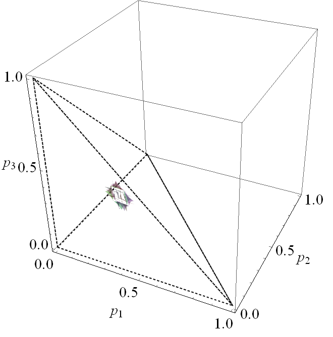
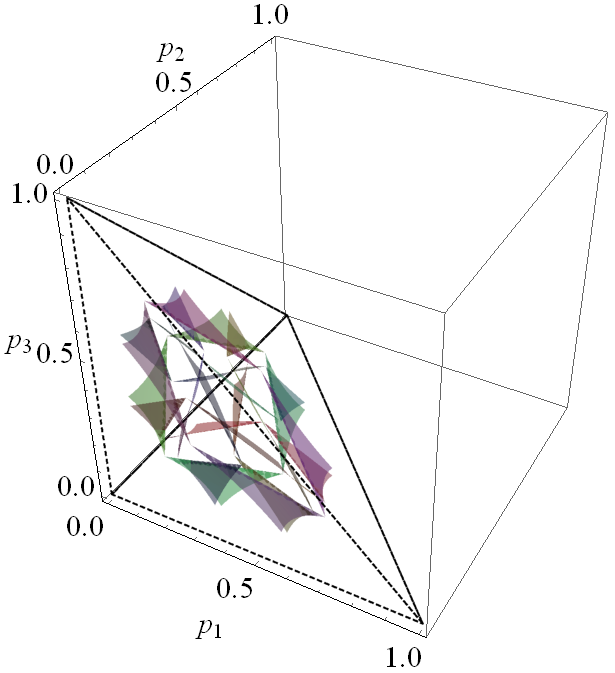
Refer to caption
Refer to caption
Refer to caption
Refer to caption
Figure 13: Probabilities for the four-level diagonal thermal equilibrium state defined by the LMG Hamiltonian for a) β=1/10𝛽110\beta=1/10, b) β=1/2𝛽12\beta=1/2, c) β=1𝛽1\beta=1, and d) β=2𝛽2\beta=2. In all the cases j=3/2𝑗32j=3/2 (ququart) and gx,gy[1,1]subscript𝑔𝑥subscript𝑔𝑦11g_{x},g_{y}\in[-1,1].

5 Summary and concluding remarks

The PME yields the Boltzmann probability distribution function for any Hamiltonian system characterizing an ensemble of particles with fixed average energy, and one is able to maximize the von Neumann entropy and minimize the Helmholtz free energy. The diagonal representation of the density matrix is a very useful tool to exhibit the purity properties of quantum systems. In this work we have considered the probability (222- and 333-simplices), the Gell-Mann, and the invariant spaces. In all of them, one is able to visualize the purity properties of qutrit and ququart systems: when there is maximum mixture, to identify the regions where the eigenvalues exhibit triple or double degeneracies, and also the loci of points where all the eigenvalues are different. In order to do that, it was necessary to establish linear and non-linear maps between the mentioned representations, which additionally allow us to determine general geometric properties of the qutrit and ququart systems such as the following: (i) trajectories in the p𝑝p-, λ𝜆\lambda-, and t𝑡t- spaces, by changing the temperature associated to the density matrix, and in this form visualize immediately the corresponding purity properties of the considered state; (ii) trajectories associated to fixed values of the invariants t2subscript𝑡2t_{2}, t3subscript𝑡3t_{3}, and t4subscript𝑡4t_{4} (see Figs. 3, 4, 6, 7). For the thermal states associated to the linear Hamiltonian in the angular momentum operators it was possible to establish: (i) For the qutrit, the curves p12=p2p3subscriptsuperscript𝑝21subscript𝑝2subscript𝑝3p^{2}_{1}=p_{2}p_{3} and its corresponding permutations giving rise to three-petal-flower-like structure in the 222-simplex, and also the corresponding mapping to the λ𝜆\lambda space; in the t𝑡t-space a trajectory with fixed values of t2subscript𝑡2t_{2} and t3subscript𝑡3t_{3} was shown (see Fig. 8); the double degeneracy happens when the Hamiltonian interaction strengths g±subscript𝑔plus-or-minusg_{\pm} describe hyperbolae with axes equal to 2ω2𝜔2\omega. (ii) For the ququart with p1p4=p2p3subscript𝑝1subscript𝑝4subscript𝑝2subscript𝑝3p_{1}p_{4}=p_{2}p_{3} and its corresponding permutations, similar geometric structures were determined, but now inside the corresponding 333-simplex (the tetrahedron). The analysis of the LMG Hamiltonian model includes the qutrit J=1𝐽1J=1 and the ququart J=3/2𝐽32J=3/2. For the qutrit, there is information of the quantum phase diagram by taking β=10𝛽10\beta=10 and changing the interaction strengths of the Hamiltonian. Additionally, one finds very different trajectories for the same temperatures β=1/20,1/2,1,2𝛽1201212\beta=1/20,1/2,1,2 when constraining the values of gx,gysubscript𝑔𝑥subscript𝑔𝑦g_{x},g_{y} in the interval [1,1]11[-1,1], in contrast to the paths when gx,gysubscript𝑔𝑥subscript𝑔𝑦g_{x},g_{y} lie in the interval [3,3]33[-3,3] (see Figs. 10, 11). For the ququart, the three-dimensional representation is established for different fixed values of g±subscript𝑔plus-or-minusg_{\pm} and different temperatures (see Fig. 12). For β=1/20,1/,1,2\beta=1/20,1/,1,2 the trajectories in the p𝑝p-space are exhibited for gx,gysubscript𝑔𝑥subscript𝑔𝑦g_{x},g_{y} in the interval [1,1]11[-1,1], and we see that they move to the boundary of the tetrahedron in a similar manner as for the qutrit case.

We studied different ways to visualize a three-level and four-level quantum system through its diagonal form and applied these methods in the study of thermal states defined by a Hamiltonian linear in the angular momentum operators and another non-linear Hamiltonian given by the LMG model. Explicitly, we reviewed some aspects of the representations of such systems by using 1) the state probabilities given by the eigenvalues of the density matrix, 2) the density matrix invariants {tn=Tr(𝝆n),n=2,3,}formulae-sequencesubscript𝑡𝑛Trsuperscript𝝆𝑛𝑛23\{t_{n}={\rm Tr}({\bm{\rho}}^{n}),n=2,3,\ldots\}, and 3) the generalized Gell-Mann parametrization.

For the linear and LMG model Hamiltonians we analyzed the different regions of the probability simplex which correspond to different sorting of the probability values and explored the behavior of the crossing between these regions when one changes the Hamiltonian parameters and also the temperature of the system.

The results above provide a much clearer understanding of the geometry and purity properties of qudit Hamiltonian systems.

References

References

  • [1] Bennett C and Shor P 1998 IEEE Transactions on Information Theory 44 2724–2742
  • [2] Nielsen M A and Chuang I L 2011 Quantum Computation and Quantum Information (Cambridge University Press)
  • [3] Werner R F 2001 Quantum Information Theory - an Invitation (Berlin, Heidelberg: Springer Berlin Heidelberg) pp 14–57 ISBN 978-3-540-44678-1
  • [4] Zoller P, Beth T, Binosi D, Blatt R, Briegel H, Bruss D, Calarco T, Cirac J I, Deutsch D, Eisert J, Ekert A, Fabre C, Gisin N, Grangiere P, Grassl M, Haroche S, Imamoglu A, Karlson A, Kempe J, Kouwenhoven L, Kröll S, Leuchs G, Lewenstein M, Loss D, Lütkenhaus N, Massar S, Mooij J E, Plenio M B, Polzik E, Popescu S, Rempe G, Sergienko A, Suter D, Twamley J, Wendin G, Werner R, Winter A, Wrachtrup J and Zeilinger A 2005 Eur. Phys. J. D 36 203–228
  • [5] Benenti G, Casati G and Strini G 2007 Principles of Quantum Computation and Information vol I, II (World Scientific)
  • [6] Grandy W T J 1997 American Journal of Physics 65 466–476 ISSN 0002-9505
  • [7] Shannon C E 1948 The Bell System Technical Journal 27 379–423
  • [8] Jaynes E T 1957 Phys. Rev. 106(4) 620–630
  • [9] Jaynes E T 1957 Phys. Rev. 108(2) 171–190
  • [10] Louisell W 1990 Quantum Statistical Properties of Radiation Wiley Classics Library (Wiley) ISBN 9780471523659
  • [11] Shore J and Johnson R 1980 IEEE Transactions on Information Theory 26 26–37
  • [12] Heims S P and Jaynes E T 1962 Rev. Mod. Phys. 34(2) 143–165
  • [13] Calixto M, Mayorgas A and Guerrero J 2021 Quantum Information Processing 20 ISSN 1573-1332
  • [14] Guerrero J, Mayorgas A and Calixto M 2022 Quantum Information Processing 21 ISSN 1573-1332
  • [15] Mayorgas A, Guerrero J and Calixto M 2023 Phys. Rev. E 108(2) 024107
  • [16] Fano U 1957 Rev. Mod. Phys. 29(1) 74–93
  • [17] Byrd M S and Khaneja N 2003 Phys. Rev. A 68(6) 062322
  • [18] Kimura G 2003 Phys. Lett. A 314 339–349 ISSN 0375-9601
  • [19] Akhtarshenas S J 2007 Opt. Spectrosc. 103 411–415
  • [20] Bertlmann R A and Krammer P 2008 J. Phys. A: Mathematical and Theoretical 41 235303
  • [21] Brüning E, Mäkelä H, Messina A and Petruccione F 2012 J. Modern Optics 59 1–20
  • [22] Procesi C 1978 Advances in Mathematics 29 219–225 ISSN 0001-8708
  • [23] Procesi C 2007 Lie Groups: An approach through Invariants and representations (Springer New York, NY)
  • [24] Curtiss D R 1918 Annals of Mathematics 19 251–278 ISSN 0003486X
  • [25] Arvind, Mallesh K S and Mukunda N 1997 J. Phys. A: Mathematical and General 30 2417
  • [26] Khanna G, Mukhopadhyay S, Simon R and Mukunda N 1997 Ann. of Phys. 253 55–82 ISSN 0003-4916
  • [27] Kuś M and Życzkowski K 2001 Phys. Rev. A 63(3) 032307
  • [28] Bengtsson I and Zyczkowski K 2006 Geometry of quantum states: An introduction to quantum entanglement (Cambridge University Press)
  • [29] Tay B A and Zainuddin H 2008 Chinese Physics Letters 25 1923
  • [30] Gerdt V P, Khvedelidze A M and Palii Y G 2014 J. of Math. Sciences 200 682–689
  • [31] Grunbaum B 2009 Configurations of Points and Lines Graduate studies in mathematics (Providence, RI: American Mathematical Society)
  • [32] Hirschfeld J W P 1986 Finite projective spaces of three dimensions Oxford Mathematical Monographs (London, England: Oxford University Press)
  • [33] Rau A R P 2021 Symmetry 13 ISSN 2073-8994 URL https://www.mdpi.com/2073-8994/13/9/1732
  • [34] Reichl L E 2016 A Modern Course in Statistical Physics 4th ed Physics textbook (Wiley) ISBN 978-3-527-41349-2
  • [35] Linden N, Popescu S and Wootters W K 2002 Phys. Rev. Lett. 89(20) 207901
  • [36] Goldstein S, Lebowitz J L, Tumulka R and Zanghì N 2006 Phys. Rev. Lett. 96(5) 050403
  • [37] Tasaki H 1998 Phys. Rev. Lett. 80(7) 1373–1376
  • [38] Coxeter H S M 1948 Regular Polytopes (Methuen & Co. Ltd., London)
  • [39] Gilmore R 2005 Lie Groups, Lie Algebras, and Some of Their Applications Dover Books on Mathematics (Dover Publications) ISBN 9780486131566
  • [40] Brüning E, Mäkelä H, Messina A and Petruccione F 2012 Journal of Modern Optics 59 1
  • [41] Lipkin H J, Meshkov N and Glick A J 1965 Nucl. Phys. 62 188
  • [42] Meshkov N, Glick A J and Lipkin H J 1965 Nucl. Phys. 62 199
  • [43] Glick A J, Lipkin H J and Meshkov N 1965 Nucl. Phys. 62 211
  • [44] Botet R, Jullien R and Pfeuty P 1982 Phys. Rev. Lett. 49(7) 478–481
  • [45] Botet R and Jullien R 1983 Phys. Rev. B 28(7) 3955–3967
  • [46] Pérez-Campos C, González-Alonso J R, Castaños O and R L 2010 Annals of Physics 325 325–344
  • [47] Kitagawa M and Ueda M 1993 Phys. Rev. A 47(6) 5138–5143
  • [48] Castaños O, López-Peña R, Nahmad-Achar E and Hirsch J G 2012 J. Phys.: Conf. Ser. 403 012003