Dynamic Anisotropic Smoothing for Noisy Derivative-Free Optimization

Abstract

We propose a novel algorithm that extends the methods of ball smoothing and Gaussian smoothing for noisy derivative-free optimization by accounting for the heterogeneous curvature of the objective function. The algorithm dynamically adapts the shape of the smoothing kernel to approximate the Hessian of the objective function around a local optimum. This approach significantly reduces the error in estimating the gradient from noisy evaluations through sampling. We demonstrate the efficacy of our method through numerical experiments on artificial problems. Additionally, we show improved performance when tuning NP-hard combinatorial optimization solvers compared to existing state-of-the-art heuristic derivative-free and Bayesian optimization methods.

1 Introduction

1.1 Problem formulation

The problem of optimizing an objective function without access to its gradient, also known as derivative-free optimization, is a well-developed field due to its widespread applications(Larson et al., 2019; Berahas et al., 2022; Gasnikov et al., 2022a). We consider derivative-free optimization problems of the form:

$$\text{argmax}_{x\in\mathbb{R}^{D}}f(x)$$ (1)

where an oracle gives us access to only noisy evaluation $\hat{f}$ to the objective function $f$ with $\hat{f}(x,\zeta)=f(x)+\zeta(x)$ and $\zeta$ some noise term which can be deterministic or stochastic bounded noise such that $\zeta(x)<\zeta_{f}$. In particular, the gradient $\nabla_{x}f$ of $f$ is unknown but is assumed to be Lipschitz-continuous.

Such problems arise notably in the field of machine learning(Schulman et al., 2015; Bogolubsky et al., 2016; Salimans et al., 2017; Choromanski et al., 2018; Liu et al., 2018) including hyper-parameter tuning (Snoek et al., 2012; Falkner et al., 2018; Bergstra et al., 2013; Akiba et al., 2019) (see review (Bischl et al., 2023)), automated architecture design(Domhan et al., 2015) and reinforcement learning (Gasnikov et al., 2022b). These problems also appear in the field of combinatorial optimization for algorithm tuning and configuration(Hutter et al., 2007, 2009, 2011; Ansótegui et al., 2009, 2015; Birattari et al., 2010; Hoos et al., 2021; Bernal, 2021; Parizy et al., 2023) and automated design of search heuristics(Khudabukhsh et al., 2009; KhudaBukhsh et al., 2016)

In this paper, we are interested in cases where the evaluation of $\hat{f}$ is computationally very costly which puts a limit on the number points $x$ that can be sampled. As a case study, we focus more particularly on the task of algorithm tuning for heuristic NP-hard combinatorial optimization (CO) solvers. These heuristics(Pincus, 1970; Lin & Kernighan, 1973; Selman et al., 1992; Leleu et al., 2019, 2021; Reifenstein et al., 2021, 2023) have typically many hyper-parameters ($D\gg 1$) that need to be tuned for maximizing their performance(Hutter et al., 2007, 2011; Hoos et al., 2021; Bernal, 2021; Parizy et al., 2023). In this case, $\hat{f}$ can be interpreted as the objective function of the underlying CO problem evaluated by the heuristic solver configured with the parameters $x$ with $x\in\mathbb{R}^{D}$. The exact choice for the definition of $\hat{f}$ includes time to solution, probability of finding the optimal solution, decision variable of reaching or given solution quality or the solution quality itself. For applications such as quadratic unconstrained binary optimization (QUBO, equivalent to the Ising problem) or boolean satisfiability (SAT), the runtime of the heuristic typically scales exponentially with problem size $N$(Karp, 2010). Due to the random initialization of the initial state of the heuristic, the evaluation of $\hat{f}$ is very noisy. From a practical perspective, we also assume that it is possible to compute multiple evaluations of $\hat{f}(x)$ in parallel such as in a GPU.

It has been recognized that the parameter space in machine learning and combinatorial optimization exhibits heterogeneous (or anisotropic) curvature properties(Sagun et al., 2016; Yao et al., 2020; Liu et al., 2023; Leleu et al., 2021; Reifenstein et al., 2023) at large problem size. The anisotropic property implies that the distribution of eigenvalues $\{\lambda_{i}\}_{i\in\mathbb{R}^{D}}$ of the Hessian matrix $\nabla^{2}f$ at proximity of its maximum ($\nabla f=0$) possesses a heavy tail, i.e., some directions have a much higher curvature than the average with a high probability. While some standard machine learning methods such as ADAM(Kingma & Ba, 2017) or second order methods(Yao et al., 2021) attempt to adapt to the heterogeneous curvatures, the question of how to achieve accurate derivative-free optimization using curvature information in a noisy environment is not fully understood and is the subject of current research(Bollapragada & Wild, 2019b; Liu et al., 2020; Yao et al., 2021; Kunstner et al., 2023; Liu et al., 2023)

1.2 New Dynamical Smoothing Approach

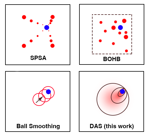
In this work, the methods of ball smoothing(Gasnikov et al., 2022b, a) and Gaussian smoothing(Nesterov & Spokoiny, 2017) for derivative-free optimization are extended to take into account the anisotropic curvature of the objective function $f$. In the new algorithm, the curvature of the smoothing kernel is dynamically adapted and converges to the Hessian matrix of the objective function $f$ at proximity of its local maxima. We prove that this dynamic sampling approach corrects for the anisotropy of the objective function which results in reduced error in the approximation of the gradient $\nabla_{x}f$ calculated from the noisy evaluations of $\hat{f}$ by the oracle. Numerical experiments on a set of artificial problems are conducted in order to demonstrate the benefits of this method. Moreover, we compare our algorithm against previously proposed derivative-free(Gasnikov et al., 2022b; Spall, 1998) and Bayesian optimization methods(Falkner et al., 2018) on the task of parameter tuning for state-of-the-art NP-hard CO heuristic solvers and show that are approach is able to tune these heuristics more optimally by taking into account the different sensitivities of each parameter.

1.3 Previous works

The line of research that inspires this work is that of derivative-free optimization. In particular, these methods are known to work well in high dimensions just like regular gradient ascent/descent although an additional $O(D)$ cost is added (Gasnikov et al., 2022b). In the presence of noise, it is not possible to get an accurate gradient using finite difference and many samples are needed to approximate the gradient. Gradient estimation can be done via finite differences(Spall, 1998), linear interpolation(Conn et al., 2009), Gaussian smoothing(Salimans et al., 2017; Nesterov & Spokoiny, 2017), and smoothing on a unit sphere(Gasnikov et al., 2022b, a). The convergence rate is given at best as $o(\frac{1}{\sqrt{n_{s}}})$ where $n_{s}$ is the number of samples(Jamieson et al., 2012). The trade-off between window size and measurement noise is investigated analytically in (Gasnikov et al., 2022b). Derivative free optimization updating an approximate Hessian has been explored in (Bollapragada & Wild, 2019a).

In addition to ball smoothing, there are many other methods that have been explored which aim to a function based on noisy measurements(Spall, 1998; Kolda et al., 2003; Kim & Zhang, 2010; Duchi et al., 2015; Conn et al., 2000; Deng & Ferris, 2006; Sun & Nocedal, 2022). Generally, these methods can be described as follows. The algorithm state is defined by some sort of sampling window which has both a position and a size. At each step, the algorithm makes noisy measurements of the objective function based on the sampling window. Then, based on the results of these samples we update the position and size of the window. Ideally, the window will shrink and the position will converge on the true optimum. The question of how to choose where to sample depending of the shape of $f$ is an open question.

There are many classes of approaches, each of which differs in exactly how the window is updated. Stochastic approximation (SA) methods such as (Spall, 1998) approximate the gradient of $f$ with what is often called a stencil. In addition to SA, direct search (DS), also known as pattern search, uses similar ideas of moving around the parameter space and zooming in (Kolda et al., 2003; Kim & Zhang, 2010). The main difference with pattern search is that typically the position is updated only when enough samples are taken to ensure the new position is better than the old one with high accuracy. This requires taking many samples in the same location. Trust region (TR) methods are another closely related method in which many samples are taken within a circular sampling window (trust region) and these samples are used to construct a model of the cost function(Conn et al., 2000; Deng & Ferris, 2006; Sun & Nocedal, 2022). Based on this model we can estimate where the minimum of the objective function is within the trust region. We then evaluate the objective function to some accuracy at the perceived optimum. Depending on how this compares to the model we then update the window size and location. Like DS, this requires taking many samples of the objective function at the model optimum in order to be certain of the new window location and shape.

Early approaches that explore adapting the sampling window size include Nelder-Mead methods are a class of algorithms in which the algorithm state is defined by a simplex of $D+1$ points. Based on function evaluations of these points the size shape and position of the simplex is updated. Originally developed by Nelder and Mead (Nelder & Mead, 1965) for noiseless functions this simplex method has been extended to noisy functions as well (Barton & Ivey, 1996). Like DS and TR, this requires many function evaluations to ensure an accurate estimate.

One line of research which is closely related to this work is the tuning for hyper-parameters for neural networks in machine learning. Research in this area has often used techniques such as Bayesian optimization to efficiently find good parameter configurations for training neural networks. These methods work by first choosing a search region over which to look for good parameters and randomly sampling points in this region. Based on these samples of the objective function we can construct a model for the true objective function and, in turn, compute what is called an acquisition function. This acquisition informs us which point will be best to sample next based on estimating how much useful information we will get by evaluating the objective at that point. Bayesian optimization is very useful when we can only evaluate the objective function a few times due to the large computational cost, however it is known to struggle in larger dimensions ($D>=20$) (Frazier, 2018). Recently many papers and libraries have used techniques from Bayesian optimization to construct algorithms designed for hyperparameter tuning. Some examples are BOHB (Bayesian optimization and hyperband) (Falkner et al., 2018), Optuna (Akiba et al., 2019), GPTune (Demmel et al., 2019) among many others. A more complete review of previous works is included in appendix section D.

2 Dynamic Window

Figure 1: Left: Cartoon depiction of different derivative-free optimization methods discussed in this work while optimizing a 2-D objective function. Red represents the distribution of sampled points while the blue dot is the optimum. Middle: Sampling window of DAS while optimizing 2-dimensional modified Rosenbrock function (see section 3.2 for details). Red ellipses represent one standard deviation of the Gaussian sampling distribution. As the algorithm progresses, the window adapts to the shape of the fitness function helping convergence. Right: Example of gradient ascent on $h(w,x)$ for a one-dimensional Gaussian fitness function in an ideal noiseless setting. The optimum is obtained by updating both window size $w$ and position $x$ according to the gradient of $h$ until the window size shrinks to 0 and $x$ converges to the optimum of $f$. This is the principle for which DIS (dynamic isotropic smoothing) and DAS (dynamic anisotropic smoothing) are based upon.

2.1 Dynamic Isotropic Smoothing Algorithm (DIS)

Before introducing the main algorithm studied in this work we will first present a simplified version which is an extension of ball smoothing (Nesterov & Spokoiny, 2017; Gasnikov et al., 2022b, a). We will refer to this algorithm as dynamic isotropic smoothing (DIS). Similar to ball smoothing, this version of the algorithm considers gradient ascent on a smoothed version of $f$:

$$h(w,x)=\frac{1}{w^{D}}\int\kappa((u-x)/w)f(u)du,$$ (2)

where the smoothing kernel $\kappa(x)$ we will define as a Gaussian $\kappa(x)=\frac{1}{(2\pi)^{D/2}}e^{-\sum_{i}x_{i}^{2}/2}$.

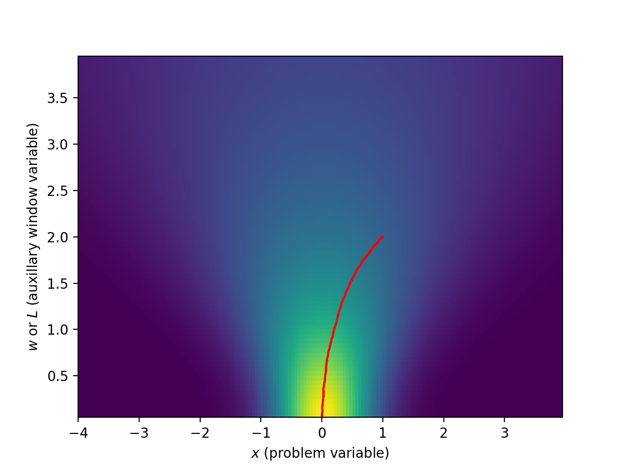
We can then consider gradient ascent on $h$ with respect to the original coordinates $x$ but also an auxiliary coordinate $w$ which represents the window size. At each step the algorithm samples randomly according to the distribution $\kappa((u-x)/w)/w$. These samples are used to estimate $\nabla h$ and then a stochastic gradient descent (ascent) algorithm is used. This allows us to simultaneously update the window size ($w$) and position ($x$) following a straightforward mathematical formulation. In the right plot of Fig. 1 we show how gradient ascent of $h$ converges on the optimum of $f$.

Next, we want to approximate $\nabla h(w,x)$ using the noisy samples of $f$ which we will denote $\hat{f}(x)$. To do this, we can first write $h_{w}(w,x)\in\mathbb{R}$ and $h_{x}(w,x)\in\mathbb{R}^{D}$ in the following integral forms.

$$h_{x}(w,x)=\int\frac{x-u}{w^{D+2}}\kappa(\frac{u-x}{w})f(u)du,$$ (3)

$$h_{w}(w,x)=\int\left(\frac{|x-u|_{2}^{2}}{w^{D+3}}-\frac{D}{w^{D+1}}\right)\kappa(\frac{u-x}{w})f(u)du.$$ (4)

These formulas express the gradient exactly, however, in practice, we only have noisy access to $f$ so clearly they cannot be computed exactly.

When we sample $v$ according to some PDF $P(v)=\frac{1}{w^{D}}\kappa((v-x)/w)$, then $h_{x}(w,x)$ and $h_{w}(w,x)$ can be computed as follows:

$$\mathbb{E}\left(f(v)\frac{x-v}{w^{2}}\right)=h_{x}(w,x),$$ (5)

and

$$\mathbb{E}\left(f(v)\left(\frac{|x-u|_{2}^{2}}{w^{3}}-\frac{D}{w}\right)\right)=h_{w}(w,x)$$ (6)

These formulas allow for the gradients to be estimated by sampling the objective function so that gradient ascent dynamics can be implemented.

2.2 Dynamic Anisotropic Smoothing Algorithm (DAS)

In this section, we will extend the dynamics of the window size to also include window shape which we will call dynamic anisotropic smoothing (DAS). In other words, the window size can contract by different amounts in different directions to properly match the fitness function’s shape. To do this, we create a new smoothed function this time parameterized by a matrix $L\in\mathbb{R}^{D}$ as:

$$h(L,x) =\int\kappa(v)f(Lv+x)dv$$ (7)

$$=\text{det}(L)\int\kappa(L^{-1}(x-u))f(u)du$$ (8)

The algorithm is constructed by approximately simulating the following dynamics:

$$\frac{dL}{dt}=\alpha_{L}\left(LL^{\top}\frac{\partial h(L,x)}{\partial L}+\lambda L+\eta_{L}\right),$$ (9)

$$\frac{dx}{dt}=\alpha_{x}\left(LL^{\top}\frac{\partial h(L,x)}{\partial x}+\eta_{x}\right),$$ (10)

where $\lambda$ is a parameter controlling the growth of the window size with $\lambda>0$. For all numerical results in section 3 and 4, we use $\lambda=0$.

The $LL^{\top}$ factor is to keep the dynamics on the correct scale when the window changes size. $\alpha_{L}$ and $\alpha_{x}$ are chosen based on the properties of the fitness function. $\eta_{L}$ an $\eta_{x}$ are noise variables associated with the imprecise measurements of the gradients.

Similar to the previous section, we can compute the partial derivatives of $h$ with respect to $L$ and $x$. We then use gradient-ascent-like dynamics to devise an algorithm that accounts for heterogeneous curvature of the fitness function (to see why this is important refer to appendix B.3).

The derivative of $h$ with respect to $L$ can be expressed as follows:

$$\frac{\partial h(L,x)}{\partial L} =(L^{-1})^{\top}M,$$ (11)

$$M_{ij} =-\int(v_{i}\kappa_{j}(v)+\delta_{ij}\kappa(v))f(Lv+x)dv$$ (12)

and with respect to $x$ as:

$$\frac{\partial h(L,x)}{\partial x}=-(L^{-1})^{\top}\int\nabla\kappa(v)f(Lv+x)dv.$$ (13)

When $\kappa$ is a Gaussian, these formulas can also be written as:

$$\frac{\partial h(L,x)}{\partial L}=(L^{-1})^{\top}\int(vv^{\top}-I)\kappa(v)f(Lv+x)dv,$$ (14)

$$\frac{\partial h(L,x)}{\partial x}=(L^{-1})^{\top}\int v\kappa(v)f(Lv+x)dv.$$ (15)

To simulate this SDE we approximate $\frac{\partial h(L,x)}{\partial L}$ and $\frac{\partial h(L,x)}{\partial x}$ using the following estimators:

$$\frac{\partial h(L,x)}{\partial L} =(L^{-1})^{\top}\mathbb{E}_{v,\zeta}(I+vv^{\top}\hat{f}(Lv+x,\zeta)),$$ (16)

$$\frac{\partial h(L,x)}{\partial x} =(L^{-1})^{\top}\mathbb{E}_{v,\zeta}(v\hat{f}(Lv+x,\zeta)).$$ (17)

Where $v$ is a Gaussian random vector and $\hat{f}(x,\zeta)$ is a noisy measurement of $f$ with random variable $\zeta$.

If we combine these concepts, we can use an Euler integration step along with the estimators to simulate the SDE (see eq. (9)) which is described in the pseudocode shown in appendix B. The parameters for this algorithm are $B_{0}$ (initial batch size), $\kappa$ (batch size exponent) and $\Delta t$ which is the integration time step as well as $\alpha_{L}$ and $\alpha_{x}$ in eq. (9). For all results in this paper, we use $\alpha_{L}=1/D$, $\alpha_{x}=1$ whereas the other parameters depend on the amount of parallelism that can be used and the properties of $f$. In this pseudo-code and in the numerical results in this work we schedule $B$ according to $\text{tr}(LL^{\top})^{\kappa/2}$ (size of the window) but other schedules can be used. The purpose of this is to use a more accurate gradient and when the window is smaller to resolve smaller and smaller values of $f$ accurately. This effect can also be achieved by manually setting a schedule for $B,\Delta t$, or both.

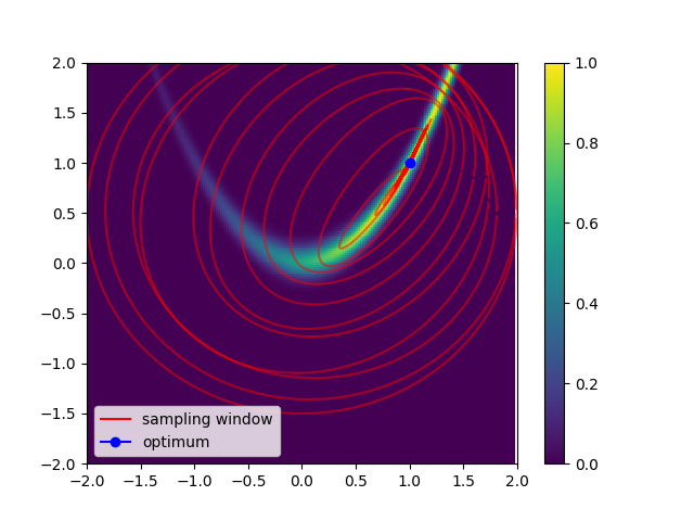
In the middle plot of Fig. 1 we show the trajectory of the sampling window for DAS in the two-dimensional modified Rosenbrock function (defined by eq. (21) in section 3.2). The sampling window starts large but as samples are collected it quickly shrinks around the nonzero region of the objective function. Because the nonzero region of the fitness function is constrained to a 1-D parabolic region, the sampling window shrinks more quickly along the axis perpendicular to the parabola. Once the window is small enough, it will begin to move along the parabola until it converges to the optimum.

2.3 Fixed Points (with $\lambda\neq 0$)

The fixed points of eq. (9) can be expressed as follows:

$$-\lambda(LL^{\top})^{-1}_{ij}=\frac{\partial}{\partial x_{i}}\frac{\partial}{\partial x_{j}}h(x,L),\quad\nabla_{x}h(x,L)=0.$$ (18)

In the limit that $\lambda\rightarrow 0$, $L\rightarrow 0$ and $x$ will approach a critical point of $f$. Moreover, $\lambda^{2}(LL^{\top})^{-1}$ will approach the hessian of $f$ at $x$. When $f$ is Gaussian, it can be shown that this fixed point corresponds to $-\lambda(LL^{\top})^{-1}=\nabla^{2}_{x}f(x)$ and $\nabla_{x}f(x)=0$ even at large window size (see appendix section A.5). Given this interpretation for $LL^{\top}$, the gradient of eq. (9) is multiplied by a pre-conditioner that converges to the inverse of the Hessian. As suggested by the literature on second-order optimization(Boyd & Vandenberghe, 2004), this type of pre-conditioner is optimal in the case of convex optimization.

2.4 Error in Gradient Estimation

The error in estimating the gradient of eq. (17) when the number of sampled points becomes large but finite is represented by the factor $\eta_{x}$ in eq. (9). It can be estimated at proximity of the maximum $\bar{x}$ of $f(x)$ and in the limit of a small window $|L|\rightarrow 0$. The central limit theorem implies that $\eta_{x}$ is normally distributed with a variance given as follows (assuming $f(\bar{x})$=1, see appendix section A.4):

$$\text{Var}[(\eta_{x})_{i}] \approx\frac{1}{n_{s}}((LL^{\top})_{ii}f(\bar{x})^{2}$$

$$+\sum_{jkl}L_{ij}^{2}(L^{\top}\nabla^{2}_{x}f(\bar{x})L)_{kl}^{2}\nu_{jkl}$$

$$-2f(\bar{x})(LL^{\top})_{ii}\sum_{j}(L^{\top}\nabla^{2}_{x}f(\bar{x})L)_{jj}$$

$$-4f(\bar{x})(L(L^{\top}\nabla^{2}_{x}f(\bar{x})L)L^{\top})_{ii}$$ (19)

where $\nu_{jkl}=2$ and $\nu_{jkl}=15$ if exactly 2 and 3 subscript indices are equal, respectively; $\nu_{jkl}=1$ otherwise.

We show in appendix A.4 that the choice of $L$ that minimizes the gradient estimation error $E$ with $E=\text{Tr}[\{\text{Cov}[(\eta_{x})_{i},(\eta_{x})_{j}]\}_{ij}]=\sum_{i}Var[(\eta_{x})_{i}]$ must form an eigenbasis of the Hessian $H$ of $f$ near the maximum $\bar{x}$. This is obtained by finding $L$ that gives $\nabla_{L}E(L)\approx 0$ when also assuming that $LL^{T}$ has a constant Frobenius norm $||L^{T}L||_{F}$. In the limit of $||L^{T}L||_{F}\rightarrow 0$, the fixed point condition $\lambda(LL^{T})^{-1}\approx\nabla_{x}^{2}f$ of eq. (18) implies that $L$ can be expressed in the same eigenbasis as the Hessian of $f$ at its maximum. In other words, the DAS algorithm converges to the kernel curvature with smallest gradient estimation error.

3 Numerical Results on Artificial Problems

3.1 Artificial Problems

If the objective function can be measured with no noise or a sufficiently small amount of noise, there are derivative-free algorithms that can work with a fixed sampling window size (Gasnikov et al., 2022b, a). That is, they estimate the gradient by measuring a few points that are close together. Because this allows for an accurate estimate of the gradient with $O(D)$ measurements, it can be shown that these methods only require $O(D)$ more samples than a regular gradient descent method (Gasnikov et al., 2022b; Nesterov & Spokoiny, 2017). In the presence of noise, this is no longer the case, however. In order to efficiently get an accurate measurement of the gradient we need to use a larger sampling window (or, in other words, the finite difference will be over a larger range). However, the gradient we get from this will not be that of the true objective function but a smoothed version of it. This biased gradient will cause the algorithm to smooth over finer details in the objective function. So, in the noisy case, there is a trade-off between large and small sampling windows which motivates the use of a dynamic sampling window which varies in size as the algorithm progresses. This trade-off is demonstrated numerically in appendix B.2. In appendix B.1 we use artificial problems to demonstrate other properties of DIS and DAS such as motivation for changing window shape (appendix B.3), and asymptotic scaling (appendix B.4).

3.2 Benchmark on Modified Rosenbrock Function

A common test function used for derivative-free optimization algorithms in the past has been Rosenbrock Function defined as

$$f(x)=\sum_{i=0}^{D-1}100(x_{i+1}-x_{i}^{2})^{2}+(1-x_{i})^{2}.$$ (20)

In this work, we will mainly study a modified version of this function in which the fitness is restricted to be in the range $[0,1]$ similar to a probability.

$$f(x)=e^{-\beta\sum_{i=0}^{D-1}100(x_{i+1}-x_{i}^{2})^{2}+(1-x_{i})^{2}}$$ (21)

This function exhibits many properties which make it hard for many algorithms to optimize. In particular, the first term (with a coefficient of 100) essentially restricts the optimal region to a parabolic manifold. Then, the optimizer will have to move along this manifold to optimize the second term which has a much more shallow gradient. Additionally, for each sample, we will randomly pick from $\{0,1\}$ with probability $f(x)$. This give the optimization problem similar characteristics to the CO parameter tuning discussed in section 4.

In Fig. 2 we show the result of applying four algorithms to this function in different dimensions and with different values of $\beta$. These numerical results are also summarized in table 1 and tables 3 and 4 of appendix B.5. As expected, in lower dimensions ($D=2$) BOHB almost always achieves the best fitness for any number of samples. However, when the dimension becomes larger, BOHB tends to struggle more and the three other methods, which are gradient based, are more effective. For the dimension $D=4$ case we can see that DAS has the best performance. Although SPSA is also effective in some cases, it can struggle from inconsistency with this type of objective function. That is, because of the discrete shape of the sampling region, many initial conditions will never be successful at all. In dimension $D=8$ all four algorithms struggle due to the large parameter space. However, with enough samples of the objective function, DAS is still able to find the optimum in many cases. For more detailed information about how DAS is implemented for the results in this section and section 4, see appendix B.

Figure 2: Fitness as a function of $n_{s}$ on the modified Rosenbrock function in different dimensions for four different algorithms. Left: $D=2,\beta=0.5$, Middle: $D=4,\beta=0.5$, Right: $D=8,\beta=0.2$. Traces are averages over 5 runs, and shaded regions represens one standard deviation of the data. Except for BOHB, each algorithm is initialized with an initial condition in $[0,1]^{D}$ and BOHB uses $[0,1]^{D}$ as the sampling window.

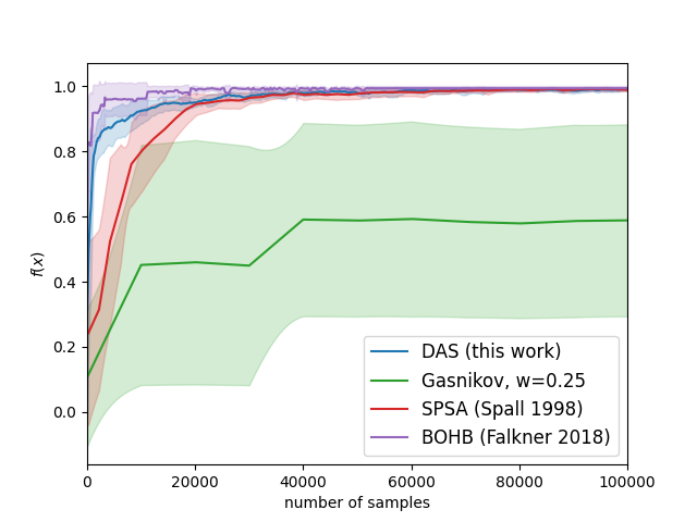
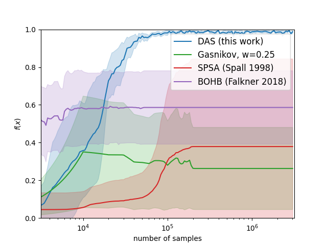
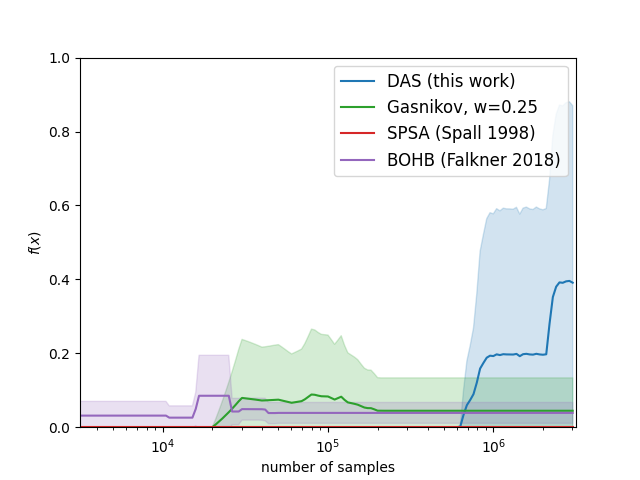
	mean	worst	best
DAS (this work)	0.981	0.962	0.994
Gasnikov, w=0.25	0.280	0.000	0.564
SPSA (Spall 1998)	0.304	0.000	0.762
BOHB (Falkner 2018)	0.586	0.243	0.796

Table 1: Table shows best, worst, and mean fitness achieved by four algorithms for $n_{s}=10^{5}$. The toy function is the modified Rosenbrock function in 4 dimensions with $\beta=0.5$.

4 Application to combinatorial optimization

4.1 Heuristic Solver Parameter Tuning

Combinatorial optimization (CO) is a type of optimization in which we look for a solution that minimizes some objective function among a set of discrete configurations. The number of possible solutions increases exponentially with the problem size and, although the objective function can be computed in polynomial time, finding optimal configuration takes an exponential amount of time in the worst case for NP-hard problems. Examples include max-cut, max-clique, Ising, TSP (traveling salesman problem), the knapsack problem, graph coloring and SAT (boolean satisfiability).

Consequently, heuristic techniques have been developed that solve typical instances of many these problems efficiently with high probability but have no strict guarantees of finding the correct solution (Pincus, 1970; Lin & Kernighan, 1973; Selman et al., 1992). More recently, a new class of heuristics, which we will call differential solvers, have been shown to be at least as efficient as state-of-the-art methods with the advantage of being well-fitted for implementation in specialized hardware accelerators(Ercsey-Ravasz & Toroczkai, 2011; Yamamoto et al., 2017; Leleu et al., 2019, 2021; Reifenstein et al., 2021, 2023; Goto et al., 2019, 2021; Kalinin et al., 2023). These heuristic algorithms typically have many parameters that need to be tuned in order to work effectively (see appendix C.1 for more details). In this section, we will compare the effectiveness of state-of-the-art tuning methods at tuning the parameters of a recently developed differential SAT solver (Reifenstein et al., 2023) (see appendix C for more details). Additionally, we have tuned a similar QUBO/Ising differential solver based on (Leleu et al., 2019) and obtain similar results (see appendix C.5).

4.2 SAT Algorithm Tuning

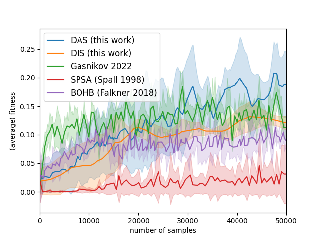
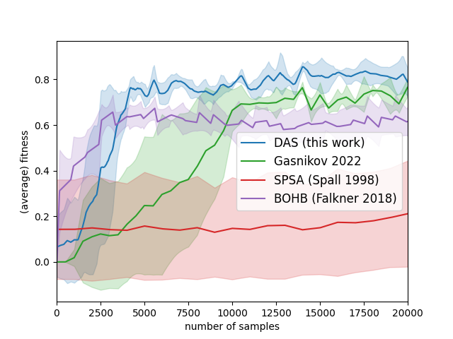
In this section, we will consider the problem of tuning the SAT solver developed in (Reifenstein et al., 2023) on random 3-SAT. This algorithm, which is described in more detail in appendix C, has four real parameters, $\text{dt},p_{init},p_{end},\beta$. We want to find the values of these parameters which maximize the success rate for a certain class of SAT problems. More specifically, for a given problem size $N$, clause to variable ratio $\alpha$, and total number of time steps $T$ there is a function of four real variables $P_{avg}(\text{dt},p_{init},p_{end},\beta)\in[0,1]$ which we wish to optimize. The noisy evaluation of this function is realized by choosing a random 3-SAT problem with the relevant parameters ($N$, $\alpha$) and computing a single trajectory of the coherent SAT solver with the given number of time steps $T$ and the given system parameters. Thus, the problem of choosing optimal parameters is a noisy derivative-free optimization problem.

In Fig. 3 we compare the performance of different optimizers discussed in this paper on tuning the SAT solver with $N=150$, $\alpha=4.0$ $T=148$. Our proposed algorithm, DAS, is able to find the best parameters. This is mostly because, unlike the other methods, it can properly account for the different sensitivities of the different parameters (see appendix C.4 for more details). One important detail to touch upon for the results in Figs. 3 (and Fig. 10 of appendix section C.4) is the optimal parameters found by DAS have very extremal values, that is, $p_{init}\approx-1$ and $\beta\approx 2$. In fact, these values are out of the search space given to BOHB which is $[0,1]^{4}$. In some sense, this is unfair to BOHB because it cannot find parameters outside of the bounds of its search. However, this is precisely one of the reasons that we believe BOHB is sub-optimal for this type of problem. Expanding the search space of BOHB to $[-1,2]^{4}$ would encompass the optimal parameters, but this adjustment would exponentially increase the search area by a factor of $3^{4}$ in the worst case, potentially leading to significant slowing down of the parameter tuning. While it is tempting to narrow the first dimension of the search box to $[0,0.3]$, based on the knowledge that the critical parameter $dt$ is optimally near $0.1$, such a strategy would inherently rely on specific prior insights. For the purpose of this discussion, we operate under the premise of minimal prior knowledge regarding the parameters, aside from a basic understanding of their magnitude. This constraint is crucial for an unbiased evaluation of a tuning method’s effectiveness, enabling its application across diverse algorithms and parameter sets without presupposed knowledge, thereby allowing for an autonomous determination of parameter sensitivities. This approach underscores the adaptability and effectiveness of the DAS method in tuning scenarios. To further emphasize the improvement provided by DAS, Fig. 3 also includes results on tuning an Ising solver. These results are discussed in more detail in appendix C.5.

Figure 3: Left: Average success probability obtained by different tuning methods on random 3-SAT with $N=150,\alpha=4.0,T=148$. Averages are over 5 realizations of the tuning dynamics starting at different randomized positions. The shaded region represents one standard deviation of the data. To evaluate the fitness of each parameter configuration, 20 random SAT instances are generated and 50 trajectories are evaluated for each. Right: A similar plot for tuning an Ising solver on problem size $N=150$ in which the performance improvement provided by DAS is clearer. This result is not discussed in the main text but is included in appendix C.5

5 Conclusion

In this work we have presented a new algorithm, which uses previous ideas from derivative-free optimization(Gasnikov et al., 2022b, a; Nesterov & Spokoiny, 2017). We have shown that it is an effective tool for the tuning of combinatorial optimization heuristic solvers. Due to its ability to adapt to a noisy objective function with heterogeneous curvature, DAS can outperform existing methods of parameter tuning(Gasnikov et al., 2022b; Spall, 1998; Falkner et al., 2018) for a variety of applications(Leleu et al., 2021; Reifenstein et al., 2023). The pros and cons of these different methods are briefly summarized in table 2. The advantage of the method for dealing with heterogenous curvature is justified analytically by the calculation of the reduction of gradient estimation error induced by the dynamic anisotropic kernel. Based on our experimentation with artificial objective functions, we believe that key properties that our target application has are: 1) heterogeneous curvature (meaning different sensitivities of parameters and correlations between parameters), 2) an objective function that evaluates to zero in most cases but is nonzero with some probability in the region of interest. We believe that in addition to combinatorial optimization, there are many other applications in which the objective function has these properties (such as the training of neural networks)(Sagun et al., 2016; Yao et al., 2020; Liu et al., 2023). Thus, our new method likely has many uses beyond what is discussed in this work.

There are also many ways in which this method can be extended to improve its effectiveness. The approach builds upon prior works by allowing additional degrees of freedom in the sampling process. Future studies could explore extensions like incorporating higher-order moments, using sums of Gaussians for the sampling window, adding momentum to gradient ascent for enhanced performance(Kingma & Ba, 2017), and employing preconditioners for a stable Hessian estimate, particularly beneficial in neural network configuration (see discussion in appendix D.3). Further, the use of common random numbers in objective function evaluations, a technique proven to boost the efficacy of derivative-free optimization methods(Agarwal et al., 2010; Shamir, 2015), presents another promising avenue for improvement.

Type of Method	Bayesian Optimization	Fixed Sampling Window	Dynamic Window Size	Dynamic Window Size and Shape
References	BOHB (Falkner et al., 2018), HyperOpt (Bergstra et al., 2013), Optuna (Akiba et al., 2019), GPTune (Demmel et al., 2019), (review (Bischl et al., 2023))	Gradient Estimator Methods (Nesterov & Spokoiny, 2017; Gasnikov et al., 2022b), (review (Gasnikov et al., 2022a; Berahas et al., 2022))	SA (stochastic approximation) (Robbins & Monro, 1951; Spall, 1998), DS (direct search) (Kolda et al., 2003; Kim & Zhang, 2010), TR (trust region methods) (Conn et al., 2000; Deng & Ferris, 2006; Sun & Nocedal, 2022), (review (Larson et al., 2019))	Modified Nelder-Mead methods (Nelder & Mead, 1965; Barton & Ivey, 1996), DAS (This Work)
Pros	Can handle noisy evaluation of non-convex function	Good for high dimensions, simple	Handles noisy function evaluations better	Can handle heterogeneous curvature of fitness function
Cons	Struggles with high dimensions	Struggles to deal with noise	Struggles with heterogeneous curvature of fitness function	Restricted to continuous search space

Table 2: Table comparing autotuning methods described in this paper.

Software and Data

Appendix A Derivation of Analytical Results

A.1 Derivation of Equations (11) and (13)

Equations (11) and (13) can be derived as follows.

$$h(L,x)=\int\kappa(v)f(Lv+x)dv\quad\rightarrow\left(\frac{\partial h(L,x)}{\partial L}\right)_{ij}=\int\kappa(v)\frac{\partial}{\partial L_{ij}}f(Lv+x)dv$$

$$=\int\kappa(v)v_{j}f_{i}(Lv+x)dv$$

This integral uses partial derivatives of $f$ which we do not have oracle access to, however, we can use integration by parts to get rid of this. First we need to substitute $u=Lv$, $du=\text{det}(L)dv$.

$$\int\kappa(v)v_{j}f_{i}(Lv+x)dv=\int\kappa(L^{-1}u)\left(\sum_{k}(L^{-1})_{jk}u_{k}\right)f_{i}(u+x)\text{det}(L)^{-1}du$$

Then we can use integration by parts on the $u_{i}$ coordinate to get:

$$=-\int\left(\frac{\partial\kappa(L^{-1}u)}{\partial u_{i}}\left(\sum_{k}(L^{-1})_{jk}u_{k}\right)+\kappa(L^{-1}u)(L^{-1})_{ji}\right)f(u+x)\text{det}(L)^{-1}du$$

$$=-\int\left(\left(\sum_{k}\kappa_{k}(L^{-1}u)(L^{-1})_{ki}\right)\left(\sum_{k}(L^{-1})_{jk}u_{k}\right)+\kappa(L^{-1}u)(L^{-1})_{ji}\right)f(u+x)\text{det}(L)^{-1}du$$

Re substituting $u=Lv$ we get:

$$=-\int\left(\left(\sum_{k}\kappa_{k}(v)(L^{-1})_{ki}\right)v_{j}+\kappa(v)(L^{-1})_{ji}\right)f(Lv+x)dv$$

$$=-\sum_{k}(L^{-1})_{ki}\int\left(\kappa_{k}(v)v_{j}+\kappa(v)\delta_{jk}\right)f(Lv+x)dv$$

A.2 Explanation of Equation (9): Scale Symmetry

Equation (9), which algorithm 2 is based upon, can be interpreted as a simple stochastic gradient ascent equation except for the extra term $LL^{\top}$ which multiplies both gradients. In this section, we will give explanations for this extra factor.

Since $LL^{\top}$ is closely related to the hessian of the fitness function (see eq. (18), one interpretation is that this matrix is a sort of preconditioner that is used to improve the numerical stability of the algorithm. It is known that using the inverse of the hessian as a preconditioner allows for much faster convergence of gradient descent-based methods. However, $LL^{\top}$ is not exactly the inverse of the hessian especially when no growth term is included.

A more concrete and complete explanation is that this factor ensures that the dynamics exhibit a sort of scale symmetry as follows. If we are given an objective function $f$ and an arbitrary nonsingular matrix $M$ we can construct the objective function $f_{M}(x)$ defined by $f_{M}(x)=f(Mx)$. Then we consider equation (9) without noise for now. That is:

$$\frac{dL}{dt}=\alpha_{L}LL^{\top}\frac{\partial h(L,x)}{\partial L},\quad\frac{dx}{dt}=\alpha_{x}LL^{\top}\frac{\partial h(L,x)}{\partial x},$$ (22)

and then consider the variable substitution $ML_{M}=L$, $Mx_{M}=x$ which gives us:

$$M\frac{dL_{M}}{dt}=\alpha_{L}\left(ML_{M}L_{M}^{\top}(M)^{\top}\frac{\partial h(ML,Mx)}{\partial L}\right)\quad M\frac{dx_{M}}{dt}=\alpha_{x}ML_{M}L_{M}^{\top}(M)^{\top}\frac{\partial h(ML_{M},Mx_{M})}{\partial x}$$

which simplifies to

$$\frac{dL_{M}}{dt}=\alpha_{L}L_{M}L_{M}^{\top}\frac{\partial h_{M}(L_{M},x_{M})}{\partial L_{M}},\quad\frac{dx_{M}}{dt}=\alpha_{x}L_{M}L_{M}^{\top}\frac{\partial h(L_{M},x_{M})}{\partial x_{M}}.$$ (23)

This tells us that the dynamics are invariant under arbitrary linear transformations which is a nice property to have. In other words, no matter how squeezed and shrunk the sampling window gets, the dynamics are in some sense identical to the original dynamics with a circular window.

A.3 Derivation of Equation (18)

Equation (18) can be derived as follows. First we will consider equation (9) with $\frac{dL}{dt}=0$ and $\frac{dx}{dt}=0$. This gives us

$$LL^{\top}\frac{\partial h(L,x)}{\partial L}+\lambda L=0$$

and

$$\nabla_{x}h(x,L)=0$$

respectively. For the first equation, we can rewrite it by considering another expression for $\frac{\partial h(L,x)}{\partial L}$ as follows.

$$h(L,x)=\int\kappa(v)f(Lv+x)dv\quad\rightarrow\left(\frac{\partial h(L,x)}{\partial L}\right)_{ij}=\int\kappa(v)\frac{\partial}{\partial L_{ij}}f(Lv+x)$$

$$\int\kappa(v)\frac{\partial}{\partial L_{ij}}f(Lv+x)=\int\kappa(v)v_{j}f_{i}(Lv+x)dv=-\int\kappa_{j}(v)f_{i}(Lv+x)dv$$

(because $\kappa$ is a Gaussian, $-v_{j}\kappa(v)=\kappa_{j}(v)$) Then we can use integration by parts on the $v_{j}$ coordinate to get:

$$-\int\kappa(v)\frac{\partial}{\partial v_{j}}f_{i}(Lv+x)dv=\int\kappa(v)\sum_{k}L_{kj}f_{ki}(Lv+x)dv$$

$$\sum_{k}L_{kj}\frac{\partial}{\partial x_{k}}\frac{\partial}{\partial x_{i}}h(L,x)=\left(\frac{\partial h(L,x)}{\partial L}\right)_{ij}$$

$$HL=\frac{\partial h(L,x)}{\partial L}$$

Where $H_{ij}=\frac{\partial}{\partial x_{i}}\frac{\partial}{\partial x_{j}}h(x,L)$ So

$$LL^{\top}HL+\lambda L=0$$

$$LL^{\top}H=-\lambda$$

A.4 Derivation error in gradient estimation

In the following, we compute the error in the estimation of the gradient when the number of sampled points become large but finite. The gradient $dx=LL^{\top}\frac{\partial h(L,x)}{\partial x}$ can be written as $dx=LL^{\top}\frac{\partial h(L,x)}{\partial x}=L\frac{1}{n_{s}}\sum_{v\in V}(v\hat{f}(Lv+x,\zeta))$ where $n_{s}$ is the number of samples and $dx$ is a sum over of many independent and identically distributed variables $v$. We set $\alpha_{x}=1$ and $dt=1$ for the sake of simplicity.

More particularly, we are interested in finding the matrix $L$ that minimizes the total error $E$ defined as follows:

$$E=\text{Tr}[\{\text{Cov}[dx_{i},dx_{j}]\}_{ij}].$$

That is to say, we are looking for $L$ such that $\nabla_{L}E=0$. Importantly, we also assume that $LL^{T}$ has a constant Frobenius norm $||L^{T}L||_{F}$, i.e., $\text{Tr}[LL^{T}]=S$, $\forall L$ with $S>0$.

The displacement $dx$ can be simplified at proximity of the maximum $\bar{x}$ of $f(x)$ and in the limit of a small window $|L|\rightarrow 0$.

First, we have:

$$f(Lv+\bar{x})=f(\bar{x})+Lv\nabla_{x}f(\bar{x})+(Lv)^{T}\nabla^{2}_{x}f(\bar{x})(Lv)+o(S^{2}),$$

with $\nabla_{x}f(\bar{x})=0$. The displacement $dx$ can be approximated as follows:

$$dx=\frac{1}{n_{s}}\sum_{v}[f(\bar{x})X(v)+Y(v)+o(S^{2})],$$

with

$$X(v) =Lv,$$ (24)

$$Y(v) =Lv[v^{\top}(L^{\top}\nabla^{2}_{x}f(\bar{x})L)v].$$ (25)

The expression for $\text{Var}[(dx)_{i}]=\text{Var}[(\eta_{x})_{i}]$ is:

$$\text{Var}[(\eta_{x})_{i}]=\frac{1}{n_{s}}[f(\bar{x})^{2}\text{Var}[X_{i}(v)]+\text{Var}[Y_{i}(v)]-2f(\bar{x})\text{Cov}[X_{i}(v),Y_{i}(v)]+o(S^{2})],$$

where $\text{Var}[X_{i}(v)]$, $\text{Var}[Y_{i}(v)]$, and $\text{Cov}[X_{i}(v),Y_{i}(v)]$ can be expressed as follows:

$$(\text{Var}[X_{i}(v)] =\sum_{j}L_{ij}^{2}f(\bar{x})^{2},$$ (26)

$$(\text{Var}[Y_{i}(v)]) =\sum_{jkl}L_{ij}^{2}(L^{\top}\nabla^{2}_{x}f(\bar{x})L)_{kl}^{2}\nu_{jkl},$$ (27)

$$(\text{Cov}[X_{i}(v),Y_{i}(v)]) =\sum_{jk}L_{ik}^{2}(L^{\top}\nabla^{2}_{x}f(\bar{x})L)_{jj}+2\sum_{jk}L_{ij}L_{ik}(L^{\top}\nabla^{2}_{x}f(\bar{x})L)_{jk}.$$ (28)

where $\nu_{jkl}=2$ and $\nu_{jkl}=15$ if exactly 2 and 3 subscript indices are equal, respectively; $\nu_{jkl}=1$ otherwise (for e.g., $\nu_{jjj}=15$, $\forall j$, and $\nu_{jll}=2$, $\forall j\neq l$). Thus, we have:

$$\text{Var}[(\eta_{x})_{i}] =\frac{1}{n_{s}}(\sum_{j}L_{ij}^{2}f(\bar{x})^{2},$$

$$+\sum_{jkl}L_{ij}^{2}(L^{\top}\nabla^{2}_{x}f(\bar{x})L)_{kl}^{2}\nu_{jkl},$$

$$-2f(\bar{x})\sum_{jk}L_{ik}^{2}(L^{\top}\nabla^{2}_{x}f(\bar{x})L)_{jj},$$

$$-4f(\bar{x})\sum_{jk}L_{ij}L_{ik}(L^{\top}\nabla^{2}_{x}f(\bar{x})L)_{jk}+o(S^{3}))),$$ (29)

which can be written as

$$\text{Var}[(\eta_{x})_{i}] =\frac{1}{n_{s}}((LL^{\top})_{ii}f(\bar{x})^{2}$$

$$+\sum_{jkl}L_{ij}^{2}(L^{\top}\nabla^{2}_{x}f(\bar{x})L)_{kl}^{2}\nu_{jkl}$$

$$-2f(\bar{x})(LL^{\top})_{ii}\sum_{j}(L^{\top}\nabla^{2}_{x}f(\bar{x})L)_{jj}$$

$$-4f(\bar{x})(L(L^{\top}\nabla^{2}_{x}f(\bar{x})L)L^{\top})_{ii}+o(S^{3}))),$$ (30)

Consequently, we have with $H=\nabla^{2}_{x}f(\bar{x})$ and $M=L^{\top}HL$:

$$\sum_{i}\text{Var}[(\eta_{x})_{i}] =\frac{1}{n_{s}}(\text{Tr}[LL^{\top}]f(\bar{x})^{2}$$

$$+\text{Tr}[LL^{\top}]\text{Tr}[(L^{\top}HL)^{2}]+\text{Tr}[J(L^{(2)}\circ M^{(2)})]$$

$$-2f(\bar{x})\text{Tr}[LL^{\top}]\text{Tr}[L^{\top}HL]$$

$$-4f(\bar{x})\text{Tr}[L(L^{\top}HL)L^{\top}]+o(S^{3})),$$ (31)

where $J$ is square matrix of ones, $L^{(2)}$ and $M^{(2)}$ element-wise square matrices $L$ and $M$, respectively.

We get using the approximation $\text{Tr}[(L^{\top}HL)^{2}]\approx\text{Tr}[L^{\top}HL]$ and $\text{Tr}[L(L^{\top}HL)L^{\top}]\approx\text{Tr}[L^{\top}L]\text{Tr}[L^{\top}HL]$):

$$\sum_{i}\text{Var}[(\eta_{x})_{i}] =\frac{1}{n_{s}}(\text{Tr}[LL^{\top}]f(\bar{x})^{2}$$

$$+\text{Tr}[LL^{\top}]\text{Tr}[L^{\top}HL]^{2}$$

$$-2f(\bar{x})\text{Tr}[LL^{\top}]\text{Tr}[L^{\top}HL]$$

$$-4f(\bar{x})\text{Tr}[L^{\top}L]\text{Tr}[L^{\top}HL]+o(S^{3})).$$ (32)

We want to know how $E=\sum_{i}\text{Var}[(\eta_{x})_{i}]$ changes after an infinitesimal change in $L$ under the constraint that the Frobenius norm $||L^{\top}L||_{F}^{2}$ remains constant, i.e., $\text{Tr}[LL^{\top}]=S$. For this, we define the following Lagrangian:

$$\mathcal{L}(L,\lambda)=E(L)+\mu(\text{Tr}[LL^{\top}]-S).$$

where $\mu$ is a scalar Lagrangian multiplier. To find $L$, we compute the gradient of $\mathcal{L}$ given as follows:

$$\nabla_{L}\mathcal{L} =\nabla_{L}E(L)+2\mu L.$$ (33)

Note that:

$$\nabla_{L}\text{Tr}[LL^{\top}] =2L,$$ (34)

$$\nabla_{L}\text{Tr}[L^{\top}HL] =2HL,$$ (35)

It implies that:

$$\nabla_{L}E[L] =\frac{1}{n_{s}}(2Lf(\bar{x})^{2}$$

$$+2L\text{Tr}[(L^{\top}HL)]^{2}+4HL\text{Tr}[LL^{\top}]\text{Tr}[(L^{\top}HL)]$$

$$-2f(\bar{x})(2L\text{Tr}[L^{\top}HL]+2HL\text{Tr}[LL^{\top}])$$

$$-4f(\bar{x})(2L\text{Tr}[L^{\top}HL]+2HL\text{Tr}[L^{\top}L]+o(S^{3})).$$ (36)

Then, $\nabla_{L}\mathcal{L}=0$ and $\nabla_{\mu}\mathcal{L}=0$ implies:

$$0 =\nabla_{L}E(L)+2\mu L,$$ (37)

$$0 =2Lf(\bar{x})^{2}+2L\text{Tr}[L^{T}HL]^{2}+4HL\text{Tr}[LL^{\top}]\text{Tr}[L^{T}HL]$$

$$-2f(\bar{x})(2L\text{Tr}[L^{T}HL]+2HL\text{Tr}[LL^{T}])-4f(\bar{x})(2L\text{Tr}[L^{T}HL]+2HL\text{Tr}[L^{T}L])+2\mu n_{s}L+o(S^{3}),$$

$$0 =2Lf(\bar{x})^{2}+2L\text{Tr}[L^{T}HL]^{2}+4HLS\text{Tr}[L^{T}HL]$$

$$-2f(\bar{x})(2L\text{Tr}[L^{T}HL]+2HLS-4f(\bar{x})(2L\text{Tr}[L^{T}HL]+2HLS)+2\mu n_{s}L+o(S^{3}),$$ (38)

Lastly, it is possible to rewrite the condition of the solutions of $\nabla_{L}\mathcal{L}=0$ and $\nabla_{\mu}\mathcal{L}=0$ as follows:

$$HL\approx\gamma^{\prime}L,$$ (40)

with $\gamma^{\prime}$ a scalar. i.e., $L$ must align with an eigenvector of the Hessian $H$ of $f$ near the maximum $\bar{x}$ (i.e., one column of $L$ is an eigenvector). More generally, $L$ aligns with all eigenvectors of forming the basis of H.

When $-\lambda(LL^{T})^{-1}=H$ at the fixed point of the dynamics of $L$ and $x$ (see eq. (18)), $L$ and $H$ align to the same set of eigenvectors. In this section, we have shown that the gradient estimation error $\sum_{i}\text{Var}[(\eta_{x})_{i}]$ is minimized when $L$ and $H$ share the set of eigenvectors. Thus, gradient estimation error is minimized at the fixed point.

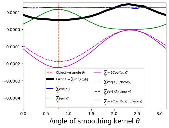
Figure 4 shows that the covariance $-{\text{Cov}[X_{i}(v),Y_{i}(v)]}_{i}$ and, in turn, the variance of $dx$ is minimized when the smoothing kernel is aligned to the curvature of the objective function. That is, the noise in the step $dx$ is minimized when the window shape matches the curvature of $f$ near its maximum.

Figure 4: Error in gradient estimation $E=\sum_{i}Var[(\eta_{x})_{i}]$ of the gradient of $x$ with $\text{Var}[(\eta_{x})_{i}]=(\text{Var}[X_{i}]+\text{Var}[X_{i}]-2\text{Cov}[X_{i},Y_{i}])$ for a Gaussian objective function $f(x)=\kappa(M(x-\bar{x}))$ centered in $\bar{x}$ and Hessian $H$ with eigenvalues $\lambda^{\prime}_{1}=1$ and $\lambda^{\prime}_{2}=4$ rotated by a reference angle $\theta_{0}$ and anisotropic smoothing kernel centered in $\bar{x}$ and curvature $(LL^{\top})^{-1}$ with with eigenvalues $\lambda_{1}=0.01$ and $\lambda_{2}=0.04$ and rotation $\theta$. The gradient estimation error $E$ is minimized for $\theta=\theta_{0}$. The dashed lines show the approximations of eq. (32). $D=2$.

A.5 Case of $f$ Gaussian with heterogeneous curvature

First note that $x$ reaches the maximum of $f$ (i.e., $\nabla_{x}h(x,L)=0)$ when $f$ is convex under the dynamics of eq. (9). This is because

$$\frac{\partial h(L,x)}{\partial x}=0\implies\frac{\partial f(x)}{\partial x}=0,$$ (41)

if $f$ is convex (i.e., $\frac{\partial f(x)}{\partial x}$ does not change sign) with

$$\frac{\partial h(L,x)}{\partial x}=\int\kappa(v)\frac{\partial f(Lv+x)}{\partial x}dv,$$ (42)

and $\kappa(v)>0$, $\forall v$.

We consider the simpler case when $f$ is a Gaussian function. In this case, we show that the dynamic window $LL^{T}$ with growth term converges to the Hessian of $f$ at its maximum (i.e., inverse of covariance matrix).

When $f$ is a Gaussian function with center $\bar{x}$ and inverse covariance matrix (Hessian) $MM^{T}$, i.e., $f(x)=\kappa(M(x-\bar{x}))$, the fixed point of eqs. (18) can be written as follows:

$$-\lambda(LL^{\top})^{-1}_{ij}=(MM^{\top})_{ij},x=\bar{x}.$$ (43)

To show eqs. (43), first note that $\frac{\partial h(L,x)}{\partial x}=0\implies\frac{\partial f(x)}{\partial x}=0$ when $f$ is Gaussian using eq. (41) and, therefore, $x=\bar{x}$ at the fixed point. Moreover, $\frac{\partial}{\partial x_{i}}\frac{\partial}{\partial x_{j}}h(L,x)=(MM^{\top})_{ij}$ at $x=\bar{x}$ because

$$\frac{\partial}{\partial x_{i}}\frac{\partial}{\partial x_{j}}h(L,x)=\int\kappa(v)\frac{\partial}{\partial x_{i}}\frac{\partial}{\partial x_{j}}\kappa(M(Lv+x-\bar{x}))dv,$$

with

$$\frac{\partial}{\partial x_{i}}\frac{\partial}{\partial x_{j}}\kappa(M(Lv+x-\bar{x}))=4(MM^{\top}(Lv+x-\bar{x}))_{i}(MM^{\top}(Lv+x-\bar{x}))_{j}\kappa(M(Lv+x-\bar{x}))-2(MM^{\top})_{ij}\kappa(M(Lv+x-\bar{x})).$$

At $x=\bar{x}$, we have

$$\int\kappa(v)(MM^{\top}(Lv))_{i}(MM^{\top}(Lv))_{j}\kappa(M(Lv))dv=0,$$

and

$$\int\kappa(v)\kappa(M(Lv))dv=1.$$

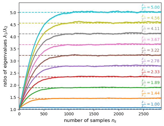
Consequently, $\frac{\partial}{\partial x_{i}}\frac{\partial}{\partial x_{j}}h(L,x)=(MM^{\top})_{ij}$. Note that this property is true whatever the window size when $f$ is Gaussian, but is not necessarily true for a general function $f$. Numerical simulations shown in Fig. 5 confirm that the Hessian of the Gaussian smoothing kernel converges to that of the function $f$ in the case $d=2$.

Figure 5: Ratio $\frac{\lambda_{1}}{\lambda_{2}}$ of the eigenvalues of the Hessian of the smoothing kernel $(LL^{\top})^{-1}$ noted $\lambda_{1}$ and $\lambda_{2}$ vs. the number of samples for various ratio $\frac{\lambda^{\prime}_{1}}{\lambda^{\prime}_{2}}$ of the Hessian of $f$ when $f$ is a Gaussian function. The dynamics converge to $\frac{\lambda_{1}}{\lambda_{2}}=\frac{\lambda^{\prime}_{1}}{\lambda^{\prime}_{2}}$. $D=2$.

Appendix B Algorithm Pseudo-Code and Numerical Stability

Algorithm 1 DAS (Dynamic Anisotropic Smoothing)

  Initialize $x,L$ {Start with $x$ as some rough guess for the parameters and $L$ large. }

  for $t\leftarrow 0$ to $T$ do

    $B=B_{0}/\text{tr}(LL^{\top})^{\kappa/2}$

    Choose $B$ random values for the random vector $v$

    SAMPLE $y_{i}=\hat{f}(Lx+v_{i})$ for each random vector (can be parrallelized)

    Using $y_{i}$, compute the estimates of $\frac{\partial h(L,x)}{\partial L}\approx\hat{h}_{L}$ and $\frac{\partial h(L,x)}{\partial x}\approx\hat{h}_{x}$ (equations (16), (17))

    Compute $\Delta L=\alpha_{L}LL^{\top}\hat{h}_{L}$, $\Delta x=\alpha_{x}LL^{\top}\hat{h}_{x}$ (equations (9))

    Set $\hat{L}\leftarrow L+\Delta t\Delta L$

    Set $\hat{\Delta t}\leftarrow\Delta t\left(\frac{|\hat{L}|}{|L|}\right)^{1/2}$ (for numerical stability)

    Set $L\leftarrow L+\hat{\Delta t}\Delta L$, $x\leftarrow x+\hat{\Delta t}\Delta x$ (update window)

    Constrain $L\leftarrow\text{CLAMP}(L)$ (for numerical stability, see equation (44) for definition of CLAMP)

  end for

  return $x$ {Return the putative best parameters}

Algorithm 2

Although the algorithm is directly based on the numerical integration of eq. (9), there are several additional steps that we add to improve numerical stability. These steps are mainly to ensure that the window size does not grow or shrink too quickly during the optimal region search. We introduce the notation $|L|=\text{tr}(LL^{\top})^{1/2}$ to denote the norm of $L$ which also represents the size of the window.

The first step is to use something like a two-step integration scheme when updating the window matrix $L$. First, we compute $\hat{L}=L+\Delta t\Delta L$ (where $\Delta L$ is the estimate of $\partial L/\partial t$) using the original time step. Then we compute a new time step: $\hat{\Delta t}\leftarrow\Delta t\frac{|\hat{L}|}{|L|}$ which we then use to update $L$ and $x$. The purpose of is to avoid the term $\Delta t\Delta L$ to become too large and negative which, in turn, will make $L$ shrink too quickly in a single time step.

Second, we limit the magnitude of $L$ so that it cannot shrink or grow too quickly. To do this, the following clamp function is applied to $L$ after each time-step:

$$\text{CLAMP}(L)=\begin{cases}L\frac{w_{max}D^{1/2}}{|L|}&|L|/D^{1/2}>w_{max}\\ L&w_{min}\leq|L|/D^{1/2}\leq w_{max}\\ L\frac{w_{min}D^{1/2}}{|L|}&|L|/D^{1/2}<w_{min}\end{cases}$$ (44)

where $w_{min}$ and $w_{max}$ are the minimum and maximum window sizes respectively. For the numerical results in this work, we always use $w_{max}=2$, and, except for the benchmark results on the Rosenbrock function (section 3.2), we use $w_{min}=0$.

B.1 Additional Numerical Results on artificial problems

Figure 6: Left: Distance from true optimum plotted against the number of oracle calls for the algorithm analyzed in (Gasnikov et al., 2022b) for different window sizes/sampling radii. The fitness function used is a 5-dimensional Gaussian function (which is symmetric). Right: $f_{opt}-f(x)$ is plotted for both (Gasnikov et al., 2022b) and algorithm 3.3. The fitness function is a piece-wise parabolic function designed to be skewed and not have reflectional symmetry.

B.2 Window Size Tradeoff

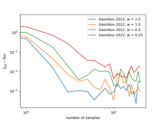
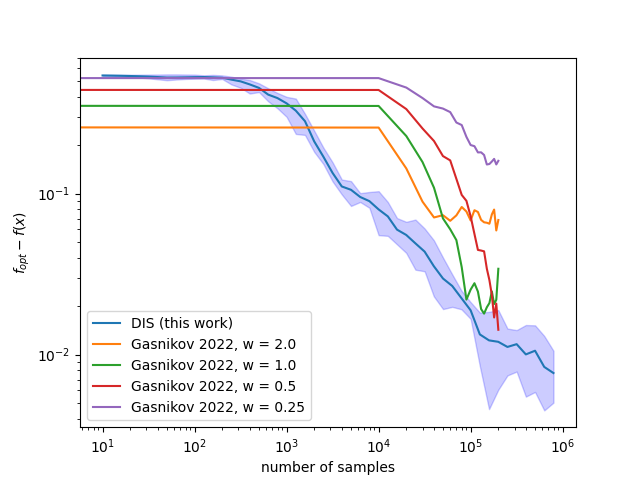
This trade-off is demonstrated numerically in Fig. 6 of appendix section B.1 in which two artificial fitness functions are optimized using the ball smoothing algorithm from (Gasnikov et al., 2022b). In the leftmost plot, we use a symmetric fitness function $f(x)=1-\frac{1}{D}\sum_{i}x_{i}^{2}$ with Gaussian noise added at each measurement. Because this function is symmetric around its optimum, a smoothed version of the function will have the same optimum, and ball smoothing can use an arbitrarily large sampling radius. Thus, the largest sampling radius ($w=2$) is most quickly able to obtain a nearly optimal configuration.

On the other hand, in the right plot of Fig. 6 we use a different, asymmetric, fitness function $f(x)=1-\frac{1}{D}\sum_{i}(1+0.9\text{sign}(x_{i}))x_{i}^{2}$. This fitness function is designed to be highly asymmetric and also not locally quadratic so it is asymmetric on small scales as well. We test both the ball smoothing algorithm from (Gasnikov et al., 2022b) as well as the DIS from section 2.1. Because of the skewed fitness function, we can see the trade-off between large and small window sizes for Gasnikov’s algorithm(Gasnikov et al., 2022b). Although a large window size such as $w=2.0$ converges faster, it converges to a sub-optimal point and the fitness does not improve after $10^{4}$ samples. This motivates the use of a dynamic window size. In fact, we can see in Fig. 6 that the DIS is always able to achieve a more optimal solution in a smaller number of samples on this fitness function. We can also see in this figure that because of the linear nature of the trace in the log-log plot that the asymptotic convergence of the error should be something like $O(n_{s}^{-c})$ for some $c$. In fact, in appendix B.4 we show numerically that the error of DAS asymptotically scales as $O(D/n_{s}^{1/2})$ which is known to be optimal for type of noisy optimization (Larson et al., 2019).

B.3 Heterogeneous curvature

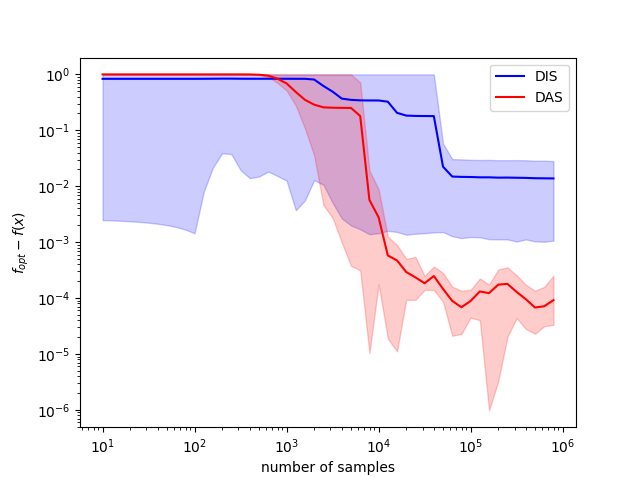
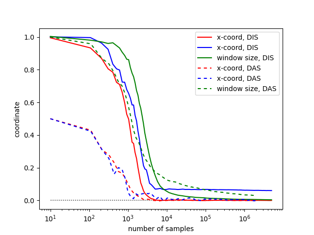
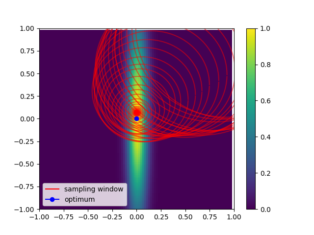
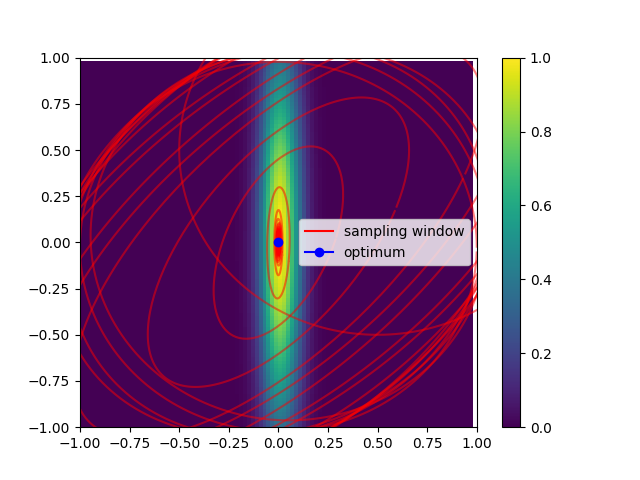
When tuning parameters, it is often the case that some parameters will have much higher sensitivity than others. This is true for the CO solvers tuned in this paper (see sections 4 and C.5) and has been commonly observed when tuning the weights of neural networks in machine learning(Bollapragada & Wild, 2019b; Yao et al., 2021; Liu et al., 2023). This phenomenon of heterogeneous curvature is the motivation behind changing the sampling window shape as described in section 2.2.

In Fig. 7, we show numerical results on the 2-dimensional fitness function $f(x,y)=e^{-100x^{2}-y^{2}}$. When a circular sampling window is used, the window size shrinks too quickly because of the sharp curvature in the $x$ direction. Because the window simultaneously shrinks in the $y$ direction, the algorithm struggles to accurately tune the less sensitive $y$ coordinate. However, if an elliptical sampling window is used, the algorithm correctly matches the shape of the objective function and treats each dimension appropriately.

Figure 7: Left: Error of DIS with respect to number of samples. Right: Single trajectory of DAS demonstrating the reason for the failure of the circular window.

Figure 8: Left: Red circles show sampling window (representing one standard deviation of the Gaussian kernel) at different points in the algorithm on top of the heatmap of the fitness function (formula shown in text). Right: Red ellipses show sampling window of DAS at different points during the algorithm’s trajectory. Data for both plots are the same as the right plot of figure 7.

B.4 Asymptotic Convergence

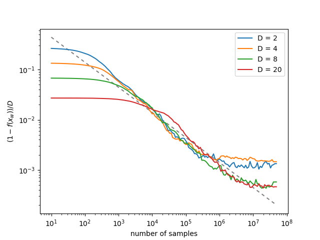
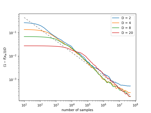
In this section, we will numerically study the asymptotic convergence rate of DAS. Let $\epsilon(n_{s})$ be the residual error in finding the true optimum of $f$ with $\epsilon(n_{s})=f_{opt}-f(x)$ obtained after $n_{s}$ samples. Then at best, $\epsilon(n_{s})=O(n_{s}^{-1/2})$(Jamieson et al., 2012). This is roughly because, due to the central limit theorem, we will need at least $\frac{\sigma^{2}}{\epsilon^{2}}$ samples to resolve $f$ to within $\epsilon$ at a single point. Many algorithms have been shown theoretically to achieve similar convergence rates on certain classes of problems (see table 8.1 of (Larson et al., 2019)).

In Fig. 9, we show the error of algorithm 2 with two different values of $\kappa$. The fitness function used for these results is $f(x)=1-\frac{1}{D}\sum_{i}(1+0.9\text{sign}(x_{i}))x_{i}^{2}$ and the measurement noise is a zero mean Gaussian with variance $0.01$. Although $\kappa=0.5$ has been used for many of the previous numerical results in 3 $\kappa=1.0$ appears to show the correct asymptotic convergence in the large $n_{s}$ limit. When $\kappa=1.0$ the algorithm appears to converge according to $\epsilon=O\left(\frac{D}{n_{s}^{1/2}}\right)$.

Figure 9: Normalized error, $\epsilon/D$, of algorithm 2 as a function of the number of samples ($n_{s}$) for different dimensions. The dotted gray line represents the function $c/n_{s}^{1/2}$ with $c=1.4$. Left: algorithm parameter $\kappa=0.5$ , right $\kappa=1.0$. Error is averaged over 5 runs for each trace. Fitness function is defined as $f(x)=1-\frac{1}{D}\sum_{i}(1+0.9\text{sign}(x_{i}))x_{i}^{2}$.

B.5 Additional Results on Modified Rosenbrock Function

Tables 3 and 4 show results from figure 2 in tabular form. Bolded numbers represent the best fitness of each column. BOHB performs better in many cases, however, in higher dimensions, DAS will always outperform BOHB with enough samples.

	$n_{s}=10^{3}$ mean	$n_{s}=10^{3}$ worst	$n_{s}=10^{3}$ best	$n_{s}=10^{4}$ mean	$n_{s}=10^{4}$ worst	$n_{s}=10^{4}$ best	$n_{s}=10^{5}$ mean	$n_{s}=10^{5}$ worst	$n_{s}=10^{5}$ best
DAS (this work)	0.734	0.549	0.852	0.925	0.861	0.981	0.993	0.982	0.997
Gasnikov, w=0.25	0.141	0.000	0.551	0.451	0.000	0.779	0.588	0.000	0.776
SPSA (Spall 1998)	0.270	0.001	0.652	0.800	0.662	0.966	0.990	0.986	0.998
BOHB (Falkner 2018)	0.902	0.775	0.996	0.963	0.868	0.999	0.994	0.980	0.999

Table 3: Table shows best, worst, and mean fitness achieved by four algorithms for different values of $n_{s}$. The artificial problem is the modified Rosenbrock function in 2 dimensions with $\beta=0.5$.

	$n_{s}=10^{4}$ mean	$n_{s}=10^{4}$ worst	$n_{s}=10^{4}$ best	$n_{s}=10^{5}$ mean	$n_{s}=10^{5}$ worst	$n_{s}=10^{5}$ best	$n_{s}=10^{6}$ mean	$n_{s}=10^{6}$ worst	$n_{s}=10^{6}$ best
DAS (this work)	0.000	0.000	0.000	0.000	0.000	0.000	0.192	0.000	0.962
Gasnikov, w=0.25	0.000	0.000	0.000	0.083	0.000	0.415	0.044	0.000	0.222
SPSA (Spall 1998)	0.000	0.000	0.000	0.000	0.000	0.000	0.000	0.000	0.000
BOHB (Falkner 2018)	0.031	0.000	0.085	0.039	0.002	0.083	0.039	0.002	0.083

Table 4: Table shows best, worst, and mean fitness achieved by four algorithms for different values of $n_{s}$. The artificial problem is the modified Rosenbrock function in 8 dimensions with $\beta=0.2$.

Appendix C Details on Combinatorial Optimization Solvers

C.1 Additional Discussion on Combinatorial Optimization

A common problem with all heuristic CO solvers, especially the differential solvers, is that there typically are many parameters that need to be optimized to ensure good performance (Leleu et al., 2019; Reifenstein et al., 2021, 2023; Goto et al., 2021; Kalinin et al., 2023). Additionally, the optimal parameters can be very different depending on the exact type of problem that is being solved (e.g. for some application-specific problem) and often vary from instance to instance as well. The problem of parameter make it hard to fairly compare different heuristics. The main motivation behind the tuning algorithm developed in this work is to be able to quickly and accurately find good parameters for these new differential solvers. This will allow us to further the development and benchmarking of them. Improving the parameter selection techniques for differential solvers will possibly allow them to be more competitive against classical heuristics in situations where they currently struggle.

The problem of tuning parameters for combinatorial optimization is not new. For example, many previous works have developed methods for tuning heuristic SAT solvers (Hutter et al., 2007, 2011; Hoos et al., 2021; Fuchs, 2023). These works focused on tuning both discrete and continuous parameters. Additionally, these works tend to use very basic methods for optimizing the continuous parameters. In our work, we focus on continuous parameters only and base our optimizer on previous results in derivative-free optimization.

More recently, due to the growing interest in Ising machines, several authors have studied methods for tuning Ising machines (Parizy et al., 2023; Bernal, 2021). Unlike our methods, these methods are more closely related to bayesian optimization. (Parizy et al., 2023) uses a Parzan tree estimator similar to that of BOHB (Falkner et al., 2018) while (Bernal, 2021) is directly based on Hyperopt (Bergstra et al., 2013).

Additionally, many authors have attempted to use machine learning directly to help solve optimization problems. For example, graph neural networks(Schuetz et al., 2022; Selsam et al., 2019) and deep neural networks(Taassob et al., 2023) have been used to learn the solutions of combinatorial optimization problems. Although these works may seem not so related at first glance, the tuning of parameters for a differential solver can be interpreted as training a recurrent graph neural network with a very small dimensional parameter space. This work touches on a deep connection between graph neural networks, reinforcement learning, differential solvers, and Ising machines.

C.2 QUBO/Ising CAC

Coherent Ising machines (CIMs) are a proposed method for solving the Ising problem in which the Ising spins are represented with analog amplitudes. Although originally proposed as an optical analog computer (Wang et al., 2013), the CIM can be simulated by numerical integration of an ODE. These ODEs typically have several parameters that need to be tuned precisely for the device to have good performance on a particular type of Ising problem.

The current state-of-the-art CIM algorithm is defined by the following ODE (Leleu et al., 2019) which we will refer to as CIM-CAC (CIM with chaotic amplitude control).

$$\frac{dx_{i}}{dt}=x_{i}(p-1-x_{i}^{2})-e_{i}\sum_{j}J_{ij}x_{j}$$ (45)

$$\frac{de_{i}}{dt}=\beta e_{i}\left(1-x_{i}^{2}\right)$$ (46)

For an Ising problem of size $N$ and coupling matrix $J_{ij}$, the algorithm evolves both $N$ dimensional vectors $x$ and $e$ over time using an Euler numerical integration step. The variables are initialized randomly, and the sign of $x$ represents the possible solution of the corresponding Ising problem. Typically many trajectories are used to find a good solution. The parameters $\beta$ and $p$ as well as the numerical integration step dt are important to tune precisely for the algorithm to be effective.

C.3 SAT-CAC

The coherent SAT solver is designed to find a variable assignment that satisfies the problem, or, if it is unsatisfiable, find an assignment that satisfies the maximum number of clauses (MAX-SAT). The SAT problem is specified by a sparse matrix $C_{ij}$ as follows:

$$C_{ij}=\left\{\begin{array}[]{ll}1&i\text{th variable is included un-negated in }j\text{th clause}\\ -1&i\text{th variable is included negated in }j\text{th clause}\\ 0&i\text{th variable is not included in }j\text{th clause}\\ \end{array}\right.$$ (47)

Then we also define the set $I_{j}$ for each clause as $I_{j}=\left\{i\mid C_{ij}\neq 0\right\}$ The boolean variables are represented by soft spins $x_{i}\in\mathbb{R}$ where $x_{i}>0$ represents True and $x_{i}<0$ represents False. Then we define the following quantities:

$$K_{j}=\prod_{i\in I_{j}}\frac{1-C_{ij}x_{i}}{2}\quad K_{ij}=\frac{-C_{ij}}{2}\prod_{k\in I_{j},k\neq i}\frac{1-C_{kj}x_{k}}{2}$$ (48)

Then, the coherent SAT solver equations can be written as:

$$\frac{dx_{i}}{dt}=x_{i}(p-1-x_{i}^{2})-e_{i}\sum_{j}K_{ij}$$ (49)

$$\frac{de_{i}}{dt}=\beta e_{i}(1-x_{i}^{2})$$ (50)

These equations are nearly identical to the CIM equations (45)(46) and thus have the same system parameters. Additionally, the parameter $p$ is typically set to change throughout the trajectory, in total there are four relevant parameters, dt, $p_{init}$, $p_{end}$, and $\beta$.

C.4 Tuning Trajectories for SAT Solver

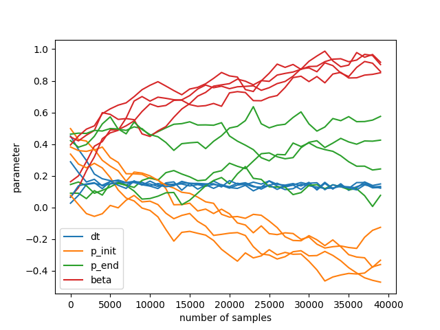
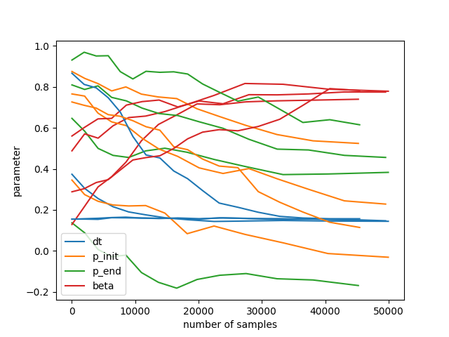
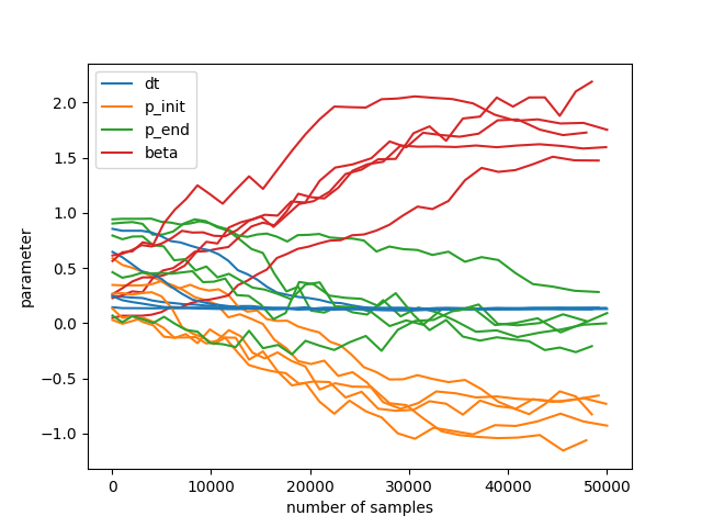
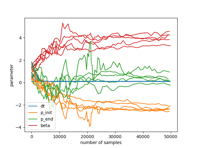
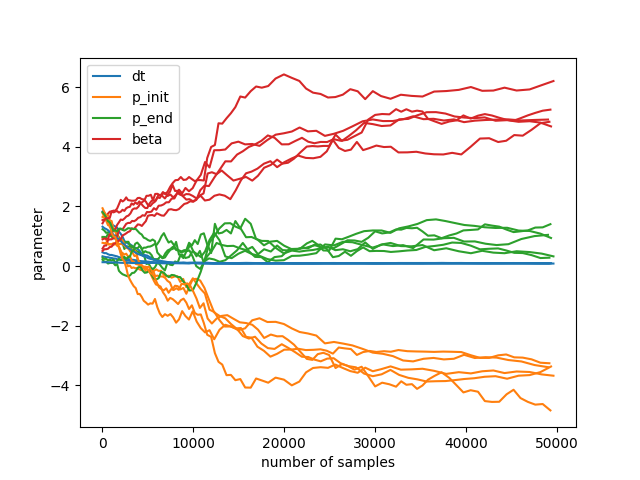
In Fig. 10, we show the trajectories of each parameter during the tuning process for three algorithms. The first algorithm (following (Gasnikov et al., 2022b)) uses a fixed sampling window with a fixed size. The second one uses a sampling window with a dynamic size but fixed shape and the third uses a dynamic size and shape as described in this work. Both the first and third algorithms converge on roughly the same parameters regardless of the initial condition, while the middle does not. This is because (as described earlier) different sensitivities to different parameters can cause the sampling window to prematurely shrink. In this case, the dt parameter is much more sensitive, so the algorithm will tune dt while neglecting the others. With a dynamic window shape, this is not a problem and we can see that all parameters appear to be tuned accurately. On the other hand, even though the Gasnikov algorithm is consistent with the parameters it chooses, these parameters are sub-optimal (see figure 3 ) because it is operating on a smoothed version of the objective function.

Figure 10: Tuning trajectories over 4-5 different initial conditions for Gasnikov et al 2022 (left), DIS (middle), and DAS (right).

C.5 Additional Results on QUBO/Ising

In this section, we consider tuning of the coherent Ising machine, which is described in detail in section C.2. A common way that Ising machines are benchmarked has been by randomly choosing values for the weight matrix. This ensemble of problem instances is known as the Sherrington-Kirkpatrick (SK) model in spin glass physics (SK). The SK model has been very well studied from the perspective of statistical physics and spin glass theory and this is one of the reasons it is commonly used as a benchmark for Ising machines. For example, the average ground state energy of an SK problem instance can be accurately approximated (Boettcher, 2010; Parisi, 1980). For an SK problem instance with entries chosen from a zero mean Gaussian the ground state will on average be:

$$E_{avg}\approx N^{3/2}(-0.761+0.7N^{-2/3})$$ (51)

ignoring some higher order finite size corrections (Boettcher, 2010). This is useful because when we randomly generate these instances we do not know their ground state or ground state energy. So, unlike with the SAT problem, we cannot use a success rate as our fitness function since we do not know when the algorithm is successful or not. However, this formula gives us a rough estimate of the ground state energy which we can use to form a different type of fitness function we will call a ”soft success rate” as follows:

$$f(x)=\mathbb{E}\left(e^{-\beta_{E}(\hat{E}-E_{thresh})}\right)$$ (52)

This formula, which is inspired by the Boltzmann factor for statistical mechanics, depends on an inverse temperature parameter $\beta_{E}$ (not to be confused with the $\beta$ in equation (46)). $\hat{E}$ is the Ising energy returned by a single trajectory for CIM-CAC and $E_{thresh}$ is set to $N^{3/2}(-0.761+0.7N^{-2/3})$. The expected value is over both initial conditions for CIM-CAC and the ensemble of SK instances. If $\beta_{E}$ is small, then this cost function is similar to the average energy returned by the solver, while if $\beta_{E}$ is large then the fitness is closer to a success rate. This success rate is not the success rate of finding the ground state but rather the success rate of finding energy under a threshold energy for a given instance. If we are interested in finding the ground state, then we will have to assume that the optimal parameters for this cost function are also useful for finding the ground state. On the other hand, if we are just interested in finding low energy states efficiently then this formula makes sense and we can choose $\beta_{E}$ appropriately.

A more in-depth study is needed to understand the properties and usefulness of this type of fitness function. In this work, we will use this cost function as an example of how our proposed algorithm can be used for tuning an Ising machine. In figure 11 we show the fitness of four tuning algorithms as a function of the number of samples. Again, BOHB (Falkner et al., 2018) and (Gasnikov et al., 2022b) with sampling window set to $w=2$ are both effective at tuning the solver. However, similar to the case of SAT (figure 3) DAS is consistently able to achieve better fitness given enough samples. This is mainly because of its ability to adjust to the different sensitivities of the different parameters. Additionally, we see in figure 12 that DAS is consistent at finding the same parameters at both problem sizes. Similar to the SAT case (figure 10 the optimal parameters appear to have very extremal values, however DAS is still able to find them accurately.

s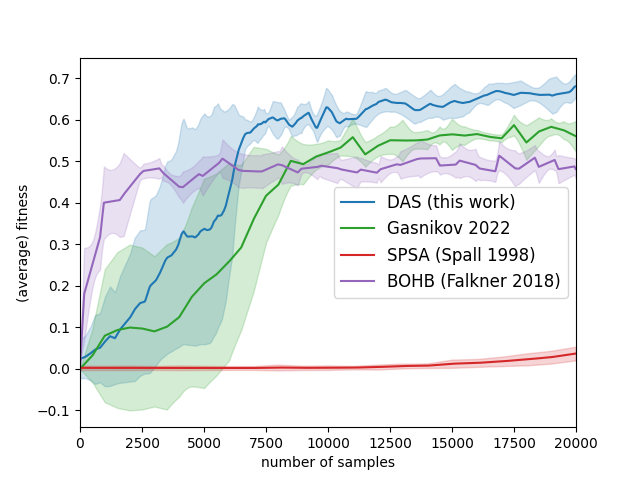

Figure 11: Average fitness (soft success rate) obtained by different tuning methods on random SK model instance with, $N=150,\beta_{E}=0.01$ (left) and $N=300,\beta_{E}=0.005$ (right). The fitness function is defined by equation (52). Averages are over 5 realizations of the tuning dynamics starting at different randomized positions. The shaded region represents one standard deviation of the data. To evaluate the fitness for each parameter configuration, 20 random SK instances are generated, and 50 trajectories are evaluated for each. The left plot of this figure is identical to the right plot of 3 of the main text but is included here as well for completeness.

Figure 12: Parameters obtained by tuning CIM-CAC with DAS on random SK model instance with, $N=150,\beta_{E}=0.01$ (left) and $N=300,\beta_{E}=0.005$ (right). The fitness function is defined by equation (52). 5 realizations of the tuning dynamics starting at different randomized positions are shown.

Appendix D Comparison with Previous Methods

D.1 Comparison to other sampling window approaches

The most common approach to derivative-free optimization is to replace the true objective function with a ”smoothed” version defined as

$$f_{\gamma}(x)=\gamma\int\kappa((x-u)/\gamma)f(u)du$$

where $\kappa$ is some convolution kernel (typically a Gaussian or a step function) (Nesterov & Spokoiny, 2017; Gasnikov et al., 2022b, a). By sampling $f$ in a region of size $\gamma$ around $x$ we can approximate the gradient of $f_{\gamma}$. When $f$ is non-differentiable or when it cannot be measured without a small amount of noise this technique is powerful because it is able to smooth over these difficulties so a traditional gradient descent method can be used.

stochastic approximation (SA) methods such as (Spall, 1998) approximate the gradient of $f$ with what is often called a stencil. That is we choose a random vector $\Delta$ from the set $\{-1,1\}^{D}$ and then approximate the gradient using the formula

$$g(x)=\Delta\frac{f(x_{k}+\Delta c_{k})-f(x_{k}-\Delta c_{k})}{2c_{k}}$$

Where $k$ is the iteration number, $x_{k}$ is the current position and $c_{k}$ is the current window size. The position is updated according to gradient descent (or ascent) as $x_{k+1}=x_{k}-a_{k}g(x_{k})$. The sequence of numbers $c_{k}$ and $a_{k}$ are set to decay with iteration number based on some function depending on the exact implementation and parameters. In this work we use the SA method described in (Spall, 1998), which we will call SPSA, to represent algorithms in this class.

D.2 Comparison to Bayesian optimization

Algorithms based on Bayesian optimization typically make use of different budgets when evaluating the objective function. That is, less accurate less, computationally intensive evaluations are combined with more computationally intensive and accurate evaluations. In this work we will use BOHB to represent this class of tuners for benchmarking purposes since it is a commonly used algorithm in the field. For a more in-depth review of Bayesian (and other types of) hyperparameter tuners we refer to (Bischl et al., 2023).

D.3 Comparison to Machine learning approaches using the Hessian

Diagonal Hessian pre-conditioning has been used in neural network optimizer design(Schaul et al., 2013) with recent iterations like AdaHessian(Yao et al., 2021). Several methods use the Gauss-Newton decomposition(Ortega & Rheinboldt, 2000) to simplify the computing the pre-conditioners in second-order optimizers(Botev et al., 2017; Gargiani et al., 2020). Other recently regularization methods proposed that improve on ADAM includes decoupled weight decay (AdamW)(Loshchilov & Hutter, 2017), Lion(Chen et al., 2023), and stochastic variance reduction(Lan & Zhou, 2018). In this paper, the focus is on tuning combinatorial heuristic but more extensive benchmarking with other methods for training neural network is the subject of future works.

D.4 Differences and Similarities between Algorithms

Although derivative-free optimization and hyper-parameter optimization are very well-developed fields, there are a number of distinct properties that our new method has which we believe make our new method unique and also optimal for the type of problems it is designed to solve. First of all, other than the Nedler-Mead-based methods, to the best of our knowledge out method is the first to use a sampling window that changes smoothly in both size and shape to fit the cost function. Having a dynamic window shape can be advantageous when some parameters have higher sensitivity than others and there are complex correlations between parameters. This is demonstrated numerically in sections 3.

Another subtle important distinction between the different algorithms is how the samples of the objective functions are taken. Methods such as DS, TR, and Nedler-Mead which are originally designed for noiseless derivative-free optimization require evaluating the objective function with high accuracy at specific points. Additionally, Bayesian methods such as BOHB also require an accurate measurement of the objective function using a high computational budget. In our case, this means sampling the objective function many times at a specific point. On the other hand, ball smoothing and SA methods use many nosy samples at many different locations to approximate the gradient and do not need to directly compare the objective function at two locations using many samples. Our method, which is most closely related to ball ball smoothing (Nesterov & Spokoiny, 2017) falls into the second class of algorithms. When many noisy objective evaluations are available and we want to get very close to the optimum in a high dimensional parameter space we believe this second class of methods is better. This is because to resolve small differences in the objective function we will need to waste computation sampling at one location many times. On the other hand, if the samples are taken at different points we can simultaneously get information about both the objective function and its gradient.

Another reason that we base our algorithm on ball smoothing is that when it comes to our target applications we want to sample points over a continuous distribution of points such as a Gaussian. The reason for this is that for many parameter configurations CO solvers have a zero or close to zero success rate. For methods that use a discrete sampling window such as SA, DS or Nelder-Mead, it is likely that the initial sampling distribution completely misses the region of the parameter space where the objective function is nonzero. With our method, we can start with a large initial sampling window and sample points according to a continuous distribution until we by chance find a good objective evaluation in the region of interest.

Table 2 summarizes the similarities and differences between different derivative-free optimization methods that we will discuss.

References

- Agarwal et al. (2010) Agarwal, A., Dekel, O., and Xiao, L. Optimal algorithms for online convex optimization with multi-point bandit feedback. In Annual Conference Computational Learning Theory, 2010. URL https://api.semanticscholar.org/CorpusID:118314530.
- Akiba et al. (2019) Akiba, T., Sano, S., Yanase, T., Ohta, T., and Koyama, M. Optuna: A next-generation hyperparameter optimization framework, 2019.
- Ansótegui et al. (2009) Ansótegui, C., Sellmann, M., and Tierney, K. A gender-based genetic algorithm for the automatic configuration of algorithms. In International Conference on Principles and Practice of Constraint Programming, pp. 142–157. Springer, 2009.
- Ansótegui et al. (2015) Ansótegui, C., Malitsky, Y., Samulowitz, H., Sellmann, M., Tierney, K., et al. Model-based genetic algorithms for algorithm configuration. In IJCAI, pp. 733–739, 2015.
- Barton & Ivey (1996) Barton, R. R. and Ivey, J. S. Nelder-mead simplex modifications for simulation optimization. Management Science, 42(7):954–973, 1996. doi: 10.1287/mnsc.42.7.954. URL https://doi.org/10.1287/mnsc.42.7.954.
- Berahas et al. (2022) Berahas, A. S., Cao, L., Choromanski, K., and Scheinberg, K. A theoretical and empirical comparison of gradient approximations in derivative-free optimization. Foundations of Computational Mathematics, 22(2):507–560, 2022.
- Bergstra et al. (2013) Bergstra, J., Yamins, D., and Cox, D. Making a science of model search: Hyperparameter optimization in hundreds of dimensions for vision architectures. In Dasgupta, S. and McAllester, D. (eds.), Proceedings of the 30th International Conference on Machine Learning, volume 28 of Proceedings of Machine Learning Research, pp. 115–123, Atlanta, Georgia, USA, 17–19 Jun 2013. PMLR. URL https://proceedings.mlr.press/v28/bergstra13.html.
- Bernal (2021) Bernal, D. Window sticker - stochastic benchmark. https://github.com/usra-riacs/stochastic-benchmark, 2021.
- Birattari et al. (2010) Birattari, M., Yuan, Z., Balaprakash, P., and Stützle, T. F-race and iterated f-race: An overview. Experimental methods for the analysis of optimization algorithms, pp. 311–336, 2010.
- Bischl et al. (2023) Bischl, B., Binder, M., Lang, M., Pielok, T., Richter, J., Coors, S., Thomas, J., Ullmann, T., Becker, M., Boulesteix, A.-L., Deng, D., and Lindauer, M. Hyperparameter optimization: Foundations, algorithms, best practices, and open challenges. WIREs Data Mining and Knowledge Discovery, 13(2):e1484, 2023. doi: https://doi.org/10.1002/widm.1484. URL https://wires.onlinelibrary.wiley.com/doi/abs/10.1002/widm.1484.
- Boettcher (2010) Boettcher, S. Simulations of ground state fluctuations in mean-field ising spin glasses. Journal of Statistical Mechanics: Theory and Experiment, 2010(07):P07002, jul 2010. doi: 10.1088/1742-5468/2010/07/P07002. URL https://dx.doi.org/10.1088/1742-5468/2010/07/P07002.
- Bogolubsky et al. (2016) Bogolubsky, L., Dvurechenskii, P., Gasnikov, A., Gusev, G., Nesterov, Y., Raigorodskii, A. M., Tikhonov, A., and Zhukovskii, M. Learning supervised pagerank with gradient-based and gradient-free optimization methods. Advances in neural information processing systems, 29, 2016.
- Bollapragada & Wild (2019a) Bollapragada, R. and Wild, S. M. Adaptive sampling quasi-newton methods for derivative-free stochastic optimization. arXiv preprint arXiv:1910.13516, 2019a.
- Bollapragada & Wild (2019b) Bollapragada, R. and Wild, S. M. Adaptive sampling quasi-newton methods for derivative-free stochastic optimization. arXiv preprint arXiv:1910.13516, 2019b.
- Botev et al. (2017) Botev, A., Ritter, H., and Barber, D. Practical gauss-newton optimisation for deep learning. In International Conference on Machine Learning, pp. 557–565. PMLR, 2017.
- Boyd & Vandenberghe (2004) Boyd, S. P. and Vandenberghe, L. Convex optimization. Cambridge university press, 2004.
- Chen et al. (2023) Chen, X., Liang, C., Huang, D., Real, E., Wang, K., Liu, Y., Pham, H., Dong, X., Luong, T., Hsieh, C.-J., et al. Symbolic discovery of optimization algorithms. arXiv preprint arXiv:2302.06675, 2023.
- Choromanski et al. (2018) Choromanski, K., Iscen, A., Sindhwani, V., Tan, J., and Coumans, E. Optimizing simulations with noise-tolerant structured exploration. In 2018 IEEE International Conference on Robotics and Automation (ICRA), pp. 2970–2977. IEEE, 2018.
- Conn et al. (2000) Conn, A., Gould, N., and Toint, P. Trust Region Methods. MOS-SIAM Series on Optimization. Society for Industrial and Applied Mathematics (SIAM, 3600 Market Street, Floor 6, Philadelphia, PA 19104), 2000. ISBN 9780898719857. URL https://books.google.com/books?id=wfs-hsrd4WQC.
- Conn et al. (2009) Conn, A. R., Scheinberg, K., and Vicente, L. N. Introduction to derivative-free optimization. SIAM, 2009.
- Demmel et al. (2019) Demmel, J. W., Li, S. X., Lakhdar, M. W. S., and USDOE. Gptune v.1, 8 2019. URL https://www.osti.gov//servlets/purl/1569031.
- Deng & Ferris (2006) Deng, G. and Ferris, M. C. Adaptation of the uobyqa algorithm for noisy functions. In Proceedings of the 38th Conference on Winter Simulation, WSC ’06, pp. 312–319. Winter Simulation Conference, 2006. ISBN 1424405017.
- Domhan et al. (2015) Domhan, T., Springenberg, J. T., and Hutter, F. Speeding up automatic hyperparameter optimization of deep neural networks by extrapolation of learning curves. In Twenty-fourth international joint conference on artificial intelligence, 2015.
- Duchi et al. (2015) Duchi, J. C., Jordan, M. I., Wainwright, M. J., and Wibisono, A. Optimal rates for zero-order convex optimization: The power of two function evaluations. IEEE Transactions on Information Theory, 61(5):2788–2806, 2015.
- Ercsey-Ravasz & Toroczkai (2011) Ercsey-Ravasz, M. and Toroczkai, Z. Optimization hardness as transient chaos in an analog approach to constraint satisfaction. Nature Physics, 7(12):966–970, 2011. doi: 10.1038/nphys2105. URL https://doi.org/10.1038/nphys2105.
- Falkner et al. (2018) Falkner, S., Klein, A., and Hutter, F. BOHB: Robust and efficient hyperparameter optimization at scale. In Dy, J. and Krause, A. (eds.), Proceedings of the 35th International Conference on Machine Learning, volume 80 of Proceedings of Machine Learning Research, pp. 1437–1446. PMLR, 10–15 Jul 2018. URL https://proceedings.mlr.press/v80/falkner18a.html.
- Frazier (2018) Frazier, P. I. A tutorial on bayesian optimization, 2018.
- Fuchs (2023) Fuchs, T. Automated tuning and portfolio selection for sat solvers. Master’s thesis, Karlsruhe Institute of Technology, 2023.
- Gargiani et al. (2020) Gargiani, M., Zanelli, A., Diehl, M., and Hutter, F. On the promise of the stochastic generalized gauss-newton method for training dnns. arXiv preprint arXiv:2006.02409, 2020.
- Gasnikov et al. (2022a) Gasnikov, A., Dvinskikh, D., Dvurechensky, P., Gorbunov, E., Beznosikov, A., and Lobanov, A. Randomized gradient-free methods in convex optimization, 2022a.
- Gasnikov et al. (2022b) Gasnikov, A., Novitskii, A., Novitskii, V., Abdukhakimov, F., Kamzolov, D., Beznosikov, A., Takac, M., Dvurechensky, P., and Gu, B. The power of first-order smooth optimization for black-box non-smooth problems. In Chaudhuri, K., Jegelka, S., Song, L., Szepesvari, C., Niu, G., and Sabato, S. (eds.), Proceedings of the 39th International Conference on Machine Learning, volume 162 of Proceedings of Machine Learning Research, pp. 7241–7265. PMLR, 17–23 Jul 2022b. URL https://proceedings.mlr.press/v162/gasnikov22a.html.
- Goto et al. (2019) Goto, H., Tatsumura, K., and Dixon, A. R. Combinatorial optimization by simulating adiabatic bifurcations in nonlinear hamiltonian systems. Science Advances, 5(4):eaav2372, 2019. doi: 10.1126/sciadv.aav2372. URL https://www.science.org/doi/abs/10.1126/sciadv.aav2372.
- Goto et al. (2021) Goto, H., Endo, K., Suzuki, M., Sakai, Y., Kanao, T., Hamakawa, Y., Hidaka, R., Yamasaki, M., and Tatsumura, K. High-performance combinatorial optimization based on classical mechanics. Science Advances, 7(6):eabe7953, 2021. doi: 10.1126/sciadv.abe7953. URL https://www.science.org/doi/abs/10.1126/sciadv.abe7953.
- Hoos et al. (2021) Hoos, H. H., Hutter, F., and Leyton-Brown, K. Chapter 12. Automated Configuration and Selection of SAT Solvers. IOS Press, February 2021. doi: 10.3233/faia200995. URL http://dx.doi.org/10.3233/FAIA200995.
- Hutter et al. (2007) Hutter, F., Hoos, H., and Stützle, T. Automatic algorithm configuration based on local search. 01 2007.
- Hutter et al. (2009) Hutter, F., Hoos, H. H., Leyton-Brown, K., and Stützle, T. Paramils: an automatic algorithm configuration framework. Journal of artificial intelligence research, 36:267–306, 2009.
- Hutter et al. (2011) Hutter, F., Hoos, H. H., and Leyton-Brown, K. Sequential model-based optimization for general algorithm configuration. In Coello, C. A. C. (ed.), Learning and Intelligent Optimization, pp. 507–523, Berlin, Heidelberg, 2011. Springer Berlin Heidelberg. ISBN 978-3-642-25566-3.
- Jamieson et al. (2012) Jamieson, K. G., Nowak, R., and Recht, B. Query complexity of derivative-free optimization. Advances in Neural Information Processing Systems, 25, 2012.
- Kalinin et al. (2023) Kalinin, K. P., Mourgias-Alexandris, G., Ballani, H., Berloff, N. G., Clegg, J. H., Cletheroe, D., Gkantsidis, C., Haller, I., Lyutsarev, V., Parmigiani, F., Pickup, L., and Rowstron, A. Analog iterative machine (aim): using light to solve quadratic optimization problems with mixed variables, 2023.
- Karp (2010) Karp, R. M. Reducibility among combinatorial problems. Springer, 2010.
- Khudabukhsh et al. (2009) Khudabukhsh, A., Xu, L., Hoos, H., and Leyton-Brown, K. Satenstein: Automatically building local search sat solvers from components. volume 232, pp. 517–524, 01 2009. doi: 10.1016/j.artint.2015.11.002.
- KhudaBukhsh et al. (2016) KhudaBukhsh, A. R., Xu, L., Hoos, H. H., and Leyton-Brown, K. Satenstein: Automatically building local search sat solvers from components. Artificial Intelligence, 232:20–42, 2016.
- Kim & Zhang (2010) Kim, S. and Zhang, D. Convergence properties of direct search methods for stochastic optimization. In Proceedings of the 2010 Winter Simulation Conference, pp. 1003–1011, 2010. doi: 10.1109/WSC.2010.5679089.
- Kingma & Ba (2017) Kingma, D. P. and Ba, J. Adam: A method for stochastic optimization, 2017.
- Kolda et al. (2003) Kolda, T. G., Lewis, R. M., and Torczon, V. Optimization by direct search: New perspectives on some classical and modern methods. SIAM Review, 45(3):385–482, 2003. doi: 10.1137/S003614450242889. URL https://doi.org/10.1137/S003614450242889.
- Kunstner et al. (2023) Kunstner, F., Chen, J., Lavington, J. W., and Schmidt, M. Noise is not the main factor behind the gap between sgd and adam on transformers, but sign descent might be. arXiv preprint arXiv:2304.13960, 2023.
- Lan & Zhou (2018) Lan, G. and Zhou, Y. An optimal randomized incremental gradient method. Mathematical programming, 171:167–215, 2018.
- Larson et al. (2019) Larson, J., Menickelly, M., and Wild, S. M. Derivative-free optimization methods. Acta Numerica, 28:287–404, 2019. doi: 10.1017/S0962492919000060.
- Leleu et al. (2019) Leleu, T., Yamamoto, Y., McMahon, P., and Aihara, K. Destabilization of local minima in analog spin systems by correction of amplitude heterogeneity. Physical Review Letters, 122, 02 2019. doi: 10.1103/PhysRevLett.122.040607.
- Leleu et al. (2021) Leleu, T., Khoyratee, F., Levi, T., Hamerly, R., Kohno, T., and Aihara, K. Scaling advantage of chaotic amplitude control for high-performance combinatorial optimization. Communications Physics, 4(1):266, 2021. doi: 10.1038/s42005-021-00768-0. URL https://doi.org/10.1038/s42005-021-00768-0.
- Lin & Kernighan (1973) Lin, S. and Kernighan, B. W. An effective heuristic algorithm for the traveling-salesman problem. Oper. Res., 21:498–516, 1973. URL https://api.semanticscholar.org/CorpusID:33245458.
- Liu et al. (2023) Liu, H., Li, Z., Hall, D., Liang, P., and Ma, T. Sophia: A scalable stochastic second-order optimizer for language model pre-training. arXiv preprint arXiv:2305.14342, 2023.
- Liu et al. (2020) Liu, L., Liu, X., Gao, J., Chen, W., and Han, J. Understanding the difficulty of training transformers. arXiv preprint arXiv:2004.08249, 2020.
- Liu et al. (2018) Liu, S., Kailkhura, B., Chen, P.-Y., Ting, P., Chang, S., and Amini, L. Zeroth-order stochastic variance reduction for nonconvex optimization. Advances in Neural Information Processing Systems, 31, 2018.
- Loshchilov & Hutter (2017) Loshchilov, I. and Hutter, F. Decoupled weight decay regularization. arXiv preprint arXiv:1711.05101, 2017.
- Nelder & Mead (1965) Nelder, J. A. and Mead, R. A Simplex Method for Function Minimization. The Computer Journal, 7(4):308–313, 01 1965. ISSN 0010-4620. doi: 10.1093/comjnl/7.4.308. URL https://doi.org/10.1093/comjnl/7.4.308.
- Nesterov & Spokoiny (2017) Nesterov, Y. and Spokoiny, V. G. Random gradient-free minimization of convex functions. Foundations of Computational Mathematics, 17:527–566, 2017. URL https://api.semanticscholar.org/CorpusID:2147817.
- Ortega & Rheinboldt (2000) Ortega, J. M. and Rheinboldt, W. C. Iterative solution of nonlinear equations in several variables. SIAM, 2000.
- Parisi (1980) Parisi, G. The order parameter for spin glasses: a function on the interval 0-1. Journal of Physics A: Mathematical and General, 13(3):1101, mar 1980. doi: 10.1088/0305-4470/13/3/042. URL https://dx.doi.org/10.1088/0305-4470/13/3/042.
- Parizy et al. (2023) Parizy, M., Kakuko, N., and Togawa, N. Fast hyperparameter tuning for ising machines. In 2023 IEEE International Conference on Consumer Electronics (ICCE), pp. 1–6, 2023. doi: 10.1109/ICCE56470.2023.10043382.
- Pincus (1970) Pincus, M. Letter to the editor—a monte carlo method for the approximate solution of certain types of constrained optimization problems. Operations Research, 18(6):1225–1228, 1970. doi: 10.1287/opre.18.6.1225. URL https://doi.org/10.1287/opre.18.6.1225.
- Reifenstein et al. (2021) Reifenstein, S., Kako, S., Khoyratee, F., Leleu, T., and Yamamoto, Y. Coherent ising machines with optical error correction circuits. Advanced Quantum Technologies, 4(11):2100077, 2021. doi: https://doi.org/10.1002/qute.202100077. URL https://onlinelibrary.wiley.com/doi/abs/10.1002/qute.202100077.
- Reifenstein et al. (2023) Reifenstein, S., Leleu, T., McKenna, T., Jankowski, M., Suh, M.-G., Ng, E., Khoyratee, F., Toroczkai, Z., and Yamamoto, Y. Coherent sat solvers: a tutorial. Adv. Opt. Photon., 15(2):385–441, Jun 2023. doi: 10.1364/AOP.475823. URL https://opg.optica.org/aop/abstract.cfm?URI=aop-15-2-385.
- Robbins & Monro (1951) Robbins, H. and Monro, S. A Stochastic Approximation Method. The Annals of Mathematical Statistics, 22(3):400 – 407, 1951. doi: 10.1214/aoms/1177729586. URL https://doi.org/10.1214/aoms/1177729586.
- Sagun et al. (2016) Sagun, L., Bottou, L., and LeCun, Y. Eigenvalues of the hessian in deep learning: Singularity and beyond. arXiv preprint arXiv:1611.07476, 2016.
- Salimans et al. (2017) Salimans, T., Ho, J., Chen, X., Sidor, S., and Sutskever, I. Evolution strategies as a scalable alternative to reinforcement learning. arXiv preprint arXiv:1703.03864, 2017.
- Schaul et al. (2013) Schaul, T., Zhang, S., and LeCun, Y. No more pesky learning rates. In International conference on machine learning, pp. 343–351. PMLR, 2013.
- Schuetz et al. (2022) Schuetz, M. J., Brubaker, J. K., and Katzgraber, H. G. Combinatorial optimization with physics-inspired graph neural networks. Nature Machine Intelligence, 4(4):367–377, 2022.
- Schulman et al. (2015) Schulman, J., Levine, S., Abbeel, P., Jordan, M., and Moritz, P. Trust region policy optimization. In International conference on machine learning, pp. 1889–1897. PMLR, 2015.
- Selman et al. (1992) Selman, B., Levesque, H., and Mitchell, D. A new method for solving hard satisfiability problems. In Proceedings of the Tenth National Conference on Artificial Intelligence, AAAI’92, pp. 440–446. AAAI Press, 1992. ISBN 0262510634.
- Selsam et al. (2019) Selsam, D., Lamm, M., Bünz, B., Liang, P., de Moura, L., and Dill, D. L. Learning a sat solver from single-bit supervision, 2019.
- Shamir (2015) Shamir, O. An optimal algorithm for bandit and zero-order convex optimization with two-point feedback. ArXiv, abs/1507.08752, 2015. URL https://api.semanticscholar.org/CorpusID:2541603.
- Snoek et al. (2012) Snoek, J., Larochelle, H., and Adams, R. P. Practical bayesian optimization of machine learning algorithms. Advances in neural information processing systems, 25, 2012.
- Spall (1998) Spall, J. Implementation of the simultaneous perturbation algorithm for stochastic optimization. IEEE Transactions on Aerospace and Electronic Systems, 34(3):817–823, 1998. doi: 10.1109/7.705889.
- Sun & Nocedal (2022) Sun, S. and Nocedal, J. A trust region method for the optimization of noisy functions, 2022.
- Taassob et al. (2023) Taassob, A., Venturelli, D., and Lott, P. A. Neural deep operator networks representation of coherent ising machine dynamics. In Machine Learning with New Compute Paradigms, 2023.
- Wang et al. (2013) Wang, Z., Marandi, A., Wen, K., Byer, R. L., and Yamamoto, Y. Coherent ising machine based on degenerate optical parametric oscillators. Phys. Rev. A, 88:063853, Dec 2013. doi: 10.1103/PhysRevA.88.063853. URL https://link.aps.org/doi/10.1103/PhysRevA.88.063853.
- Yamamoto et al. (2017) Yamamoto, Y., Aihara, K., Leleu, T., Kawarabayashi, K.-i., Kako, S., Fejer, M., Inoue, K., and Takesue, H. Coherent ising machines—optical neural networks operating at the quantum limit. npj Quantum Information, 3(1):49, 2017. doi: 10.1038/s41534-017-0048-9. URL https://doi.org/10.1038/s41534-017-0048-9.
- Yao et al. (2020) Yao, Z., Gholami, A., Keutzer, K., and Mahoney, M. W. Pyhessian: Neural networks through the lens of the hessian. In 2020 IEEE international conference on big data (Big data), pp. 581–590. IEEE, 2020.
- Yao et al. (2021) Yao, Z., Gholami, A., Shen, S., Mustafa, M., Keutzer, K., and Mahoney, M. Adahessian: An adaptive second order optimizer for machine learning. In proceedings of the AAAI conference on artificial intelligence, volume 35, pp. 10665–10673, 2021.