SSUMamba: Spatial-Spectral Selective State Space Model for Hyperspectral Image Denoising

Abstract

Denoising is a crucial preprocessing procedure for hyperspectral images (HSIs) due to the noise originating from intra-imaging mechanisms and environmental factors. Utilizing domain knowledge of HSIs, such as spectral correlation, spatial self-similarity, and spatial-spectral correlation, is essential for deep learning-based denoising. Existing methods are often constrained by running time, space complexity, and computational complexity, employing strategies that explore these kinds of domain knowledge separately. While these strategies can avoid some redundant information, they inevitably overlook broader and more in-depth long-range spatial-spectral information that positively impacts image restoration. This paper proposes a Spatial-Spectral Selective State Space Model-based U-shaped network, Spatial-Spectral U-Mamba (SSUMamba), for hyperspectral image denoising. The SSUMamba can exploit complete global spatial-spectral correlation within a module thanks to the linear space complexity in State Space Model (SSM) computations. We introduce a Spatial-Spectral Alternating Zigzag Scan (SSAZS) strategy for HSIs, which helps exploit the continuous information flow in multiple directions of 3-D characteristics within HSIs. Experimental results demonstrate that our method outperforms comparison methods. The source code is available at https://github.com/lronkitty/SSUMamba.

I Introduction

Hyperspectral images (HSIs) provide not only spatial but also detailed material information through the continuous spectral bands they capture. HSIs have been extensively used in material recognition [1], object detection [2, 3, 4], object tracking [5, 6], change detection [7], and environment protection [8]. During the acquisition of hyperspectral data, various factors such as insufficient exposure time, mechanical vibrations of imaging platforms, atmospheric perturbations, stochastic errors in photon counting, and other intrinsic and extrinsic elements inevitably introduce noise to the images [9, 10]. This noise interferes with the interpretation and application of HSIs. Hence, denoising stands as a pivotal preprocessing stage, enhancing image quality and bolstering the practical utility of high-level computer vision tasks in HSIs.

Deep learning-based denoising methods have recently garnered undivided attention. By leveraging data-driven learning, these methods can learn the 3-D nature of HSIs with spectral and spectral information. Due to the challenges posed by the design of methodology, running time, and spatial and computational complexity, existing deep learning-based methods often decompose this 3-D nature into several distinct domains for exploration, such as spatial self-similarity, spectral correlation, and local spatial-spectral correlation. For example, recurrent neural networks (RNNs) and convolutional neural networks (CNNs) are resorted to exploiting spectral correlation and local spatial-spectral correlation, respectively [11]. Moreover, attention mechanisms are concatenated to CNNs to capture spatial self-similarity further [12]. Transformer-based methods are also employed to capture long-range correlation in HSIs [9, 13, 13]. However, suffering from the $\text{O}(n^{2})$ complexity of the self-attention mechanism, these methods incorporate multiple modules to explore different kinds of domain knowledge, respectively, to reduce the length of tokens and avoid redundant information.

Figure 1: Comparison of the proposed SSUMamba and transformer-based TRQ3D and SST on the ICVL testing set. SSUMamba was evaluated using a varying number of parameters. The results indicate that SSUMamba outperforms transformer-based methods in peak signal-to-noise ratio (PSNR) while utilizing fewer parameters and memory consumption per batch.

However, given the 3-D nature of HSIs, which demonstrate spatial continuity and spectral correlation, it is essential to explore the complete global spatial-spectral correlation, especially in image restoration tasks where detailed information tends to degrade. Broader and more in-depth long-range spatial-spectral information has a positive impact that should be considered. The State Space Model (SSM) [14, 15], an approach rooted in control systems, has attracted attention for its linear complexity in handling long input sequences. Recently, Mamba [14], an optimization for SSM, has shown unique advantages in computer vision tasks [16, 17], while its linear complexity offers promising advantages in spatial correlation modeling in images. In order to further enhance Mamba’s adaptability to vision tasks, strategies like bidirectional scanning [18] and zigzag scanning [19] have been proposed. These methods enable SSM to scan image data seamlessly and comprehensively. In the field of HSI denoising, Liu et al. [20] introduced a SSM-based method for HSI denoising to exploit the bidirectional spatial information in HSIs. However, how to apply the SSM to HSIs denoising to capture the global spatial-spectral correlation following the 3-D nature of HSIs remains an open question.

This paper presents SSUMamba, a Spatial-Spectral Selective SSM-based method for denoising HSI. To address the discrepancy between HSI and sequence data, we introduce Spatial-Spectral Alternating Zigzag Scan (SSAZS) Mamba, aimed at enhancing local texture exploration and mitigating unidirectional dependency issues in SSM. We apply a spatial-spectral zigzag scan to 3-D HSI data, enabling SSM to explore information flow more continuously. Then, we extend the spatial-spectral zigzag scan to the SSAZS strategy, facilitating information flow modeling in multiple directions in HSIs. Based on the SSAZS strategy, the revised Mamba block further incorporates residual blocks to model local spatial-spectral correlation and enhance local texture exploration, along with a bidirectional Mamba layer to improve information flow. Additionally, we propose a U-shaped network architecture, SSUMamba, to leverage multi-scale features and restore HSIs. Experimental results demonstrate superior performance compared to other methods. In summary, the contributions of this work can be outlined as follows:

• The linear complexity of the Selective State Space Model (SSM) enables the modeling of global spatial-spectral correlation for HSI denoising.

• To tackle the difference between HSI data and sequence data, we introduce the Spatial-Spectral Alternating Zigzag Scan (SSAZS) strategy. It allows Mamba blocks to exploit continuous information flows in all directions, enhancing the 3-D characteristics of HSIs.

• Revised Mamba block incorporates residual blocks to model local spatial-spectral correlation and a bidirectional Mamba layer to improve information flow.

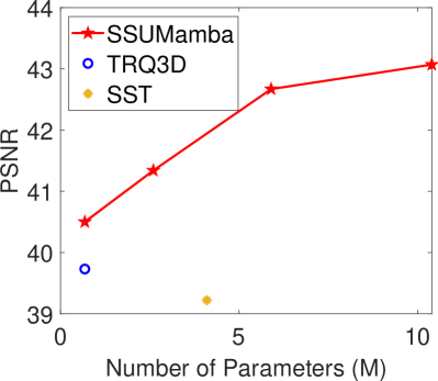
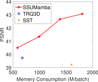
• Building upon the SSAZS Mamba block, we propose a multi-scale SSM-based network, Spatial-Spectral U-Mamba (SSUMamba), for HSI denoising. Experiments demonstrate that SSUMamba achieves better denoising results with fewer parameters and memory consumption per batch than transformer-based methods (as shown in Fig. 1).

The remainder of this article is organized as follows. Section II reviews related works. Section III introduces the details of the proposed SSUMamba. Section IV presents quantitative and visual experiments. Finally, Section V concludes this article.

II Related Work

In this section, we offer a thorough review of HSI denoising, covering both model-based, CNN-based, and transformer-based methods. We also introduce the SSM in computer vision.

II-A Model-based HSI Denoising

Conventional model-based methods exploit sparse and low-rank representations to describe the physical properties of clean hyperspectral images (HSIs) for denoising [12, 21, 22, 23, 24, 25]. For example, BM4D [26], an extension of BM3D [26], utilizes collective sparse representation to capture similarity among nonlocal spatial-spectral cubes. LLRT [27] incorporates an analysis-based hyper-Laplacian prior into the low-rank model, effectively restoring HSIs while preserving their spectral structure. NGMeet [28] uses low-rank Tucker decomposition and matrix rank minimization to capture global spectral correlation and nonlocal self-similarity, respectively. FastHyDe [29] captures spatial-spectral representations by exploiting their sparse, low-rank, and self-similarity characteristics in subspaces. E-3DTV [30] discerns global correlations and local differences across all bands by evaluating the sparsity of gradient maps in subspaces. These model-based approaches typically involve iterative optimization and manual hyperparameter fine-tuning, making them computationally inefficient and less practical for HSI denoising. Some methods have been proposed to combine model-based methods with data-driven learning [31, 32]. However, the inherent design for specifically noise types of the model makes it difficult for these methods to meet the requirements in real-world scenarios where multiple types of noise are present.

II-B CNN-based HSI Denoising

Since CNN showed its power in image denoising [33], deep learning has emerged as a critical approach in HSI denoising due to its robust learning capabilities [34]. Techniques utilizing 3-D convolution and its variations [35, 36, 11] have played a crucial role in capturing local spatial-spectral correlations for HSI denoising. Liu et al. [35] use a 3-D atrous CNN to expand the receptive field for HSI denoising, effectively handling mixture noise types while preserving image details. QRNN3D [11] integrates a recurrent unit after 3-D convolutions to leverage local spatial-spectral and global spectral correlation (GSC). NSSNN [37] combines an attention mechanism with the recurrent unit to extract GSC and non-local spatial features, achieving promising denoising performance. However, due to the limited long sequence modeling capability of CNNs, these methods often fail to capture the complete global spatial-spectral correlation, leading to suboptimal exploitation of 3-D HSIs.

II-C Transformer-based HSI Denoising

Transformers have shown remarkable success in various aspects of hyperspectral information processing, such as classification [38, 39, 40, 41, 42] and image recovery [43, 44, 45]. Hyperspectral imaging inherently involves 3-D data, where all dimensions exhibit strong correlations. While 3-D CNNs have traditionally been used for HSI modeling, the 3-D transformer [46] emerges as a promising alternative. However, suffering from the $\text{O}(n^{2})$ complexity of the self-attention mechanism, the 3-D transformer is often constrained since as the number of bands and image size increase, there is an explosion of space and computation. To address this issue, some methods use the transformer block to capture one of the long-range correlations. TRQ3D [13] incorporates a shifted windowing scheme to model nonlocal spatial relations and let RNNs model the spectral correlation. HSI-BERT [47] directly employs bidirectional encoder representations from transformers (BERTs) to encode semantic context-aware representations within all bands in each pixel to capture spectral correlation. Furthermore, SST [9] utilizes a spatial transformer to model spatial correlation and a spectral transformer to model spectral correlation. However, limited by hardware conditions and the square growth of the transformer, we have always had difficulty in realizing global spatial-spectral correlation modeling in an all-in-one manner based on the transformer.

II-D State Space Model

Recent advancements in the state space model (SSM) [15, 14] have made it widely applicable and opened up a new path for modeling sequentiality. Drawing on the theoretical basis of classical SSM from control theory and leveraging the advantages of modern deep learning, emerging deep SSMs enable efficient computation in learning long-range dependencies over extremely long timesteps. The field of computer vision has also seen an influx of SSM-based approaches [16, 18, 48, 49]. Liu et al. [16] introduced a vision Mamba block with a 2-D selective scan scheme to model the information flow in cross directions. Shi et al. [50] further proposed an omni selective scan mechanism to model information flows to include the feature dimensions. The zigzag scan [19] was introduced to enhance the continuity of information flow. SSM in HSI modeling has been widely explore [51, 52]. Liu et al. [20] apply the SSM to HSI denoising to exploit the bidirectional spatial information. However, the application of SSM to exploit the global spatial-spectral correlation in HSIs denoising remains unexplored.

Figure 2: SSUMamba uses the encoder-decoder framework, incorporating a feature extractor, encoder blocks, Spatial-Spectral Alternating Zigzag Scan (SSAZS) Mamba blocks, decoder blocks with skip connections, and a reconstructor.

Figure 3: The introduced SSAZS Mamba block, which contains residual blocks and a bidirectional SSAZS Mamba layer.

Figure 4: The introduced Spatial-Spectral Alternation Zigzag Scan (SSAZS) (c-h) in a HSI (a) with a shape of $3\times 3\times 3$. The sweep scan in Mamba is shown as (b). We first introduce the spatial-spectral zigzag scan (c) strategy in the 3-D data of HSIs, allowing the SSM to explore the information flow more continuously. We then expand the spatial-spectral zigzag scan to the SSAZS strategy for HSI data, which helps model the information flow in multiple directions from (c) to (h) in HSIs.

III Method

In this section, we first introduce the preliminaries of SSM and Mamba. Then, we provide a detailed exposition of the proposed SSUMamba, including the overall architecture, the Spatial-Spectral Alternating Zigzag Scan (SSAZS) Mamba block, and the design details.

III-A Preliminarie: State Space Models

State Space Models (SSMs) are conceptualized using continuous systems that map a one-dimensional sequence $x(t)\in\mathbb{R}^{L}$ to the output response $y(t)\in\mathbb{R}^{M}$. The SSM is defined by the following ordinary differential equation (ODE):

$$h^{\prime}(t) =Ah(t)+ Bx(t)$$ (1)

$$y(t) =Ch(t)+ Dx(t)$$

where $h(t)\in\mathbb{R}^{N}$ is the hidden state, $A\in\mathbb{R}^{N\times N}$, $B\in\mathbb{R}^{N\times L}$, $C\in\mathbb{R}^{M\times N}$, and $D\in\mathbb{R}^{M\times L}$ are the parameters of the SSM. The hidden state $h(t)$ is updated by the input $x(t)$ and the previous hidden state $h(t-1)$, and the output $y(t)$ is generated by the hidden state $h(t)$ and the input $x(t)$.

Following [15], we consider the case of a single-input single-output system, where $L=M=1$, and omit the $Dx(t)$ term. The ODE in Eq. (1) can be discretized using the zeroth-ord hold (ZOH) as follows:

$$h_{t} =\bar{A}h_{t-1}+\bar{B}x_{t}$$ (2)

$$y_{t} =\bar{C}h_{t}$$

where $\bar{A},\bar{B}$ are discrete parameters from $A,B$ as follows:

$$\bar{A} =e^{\Delta A}$$ (3)

$$\bar{B} =(\Delta A)^{-1}(e^{\Delta A}-I)\cdot\Delta B$$

where $\Delta$ is sampling step.

As we can see, Eq. (2) can be computed similarly to RNNs. To further accelerate the computation, Gu et al. [15] unroll the computation of the SSM into a convolution formulated as follows:

$$\text{y}=\text{x}\ast\bar{\text{K}}$$ (4)

where $\bar{\text{K}}=(C\bar{B},C\bar{A}\bar{B},C\bar{A}^{2}\bar{B},\cdots,C\bar{A}^{k-1}\bar{B})$ is the kernel of the convolution, $\ast$ denotes the convolution operation, and $k$ is the sequence length of input.

In Eq (2), parameters are fixed within all time steps. Gu et al. [14] introduce the Mamba as a method to optimize the parameters of SSM in a selective scan mechanism:

$$\bar{A},\bar{B}=\text{discretize}(\Delta,A,B)$$ (5)

$$y=\text{SSM}(\bar{A},\bar{B},C)(x)$$

where $x,y\in\mathbb{R}^{L\times D}$ are the input and output, respectively. $A\in\mathbb{R}^{D\times N}$ is fixed with diagonal initialization. Parameters $B,C\in\mathbb{R}^{L\times N}$, and $\Delta\in\mathbb{R}^{L\times D}$ are learned in the end-to-end training, $L$ is a length dimension, $D$ and $N$ are numbers of channels. The $\text{discretize}(\cdot)$ is the discretize procedure in [14]. Gu et al. [14] also propose hardware-aware optimization to ensure its efficient implementation.

In this paper, we follow the Mamba framework proposed in [14] and apply it to spatial-spectral modeling processing for HSI denoising.

III-B Overview Architecture

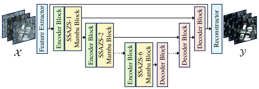
To recover the global spatial-spectral correlation and enhance the 3-D characteristics of HSIs in denoising, we propose the SSUMamba, as shown in Fig. 2. Let $\mathcal{Y}\in\mathbb{R}^{\text{B}\times\text{H}\times\text{W}}$ be a clean HSI with $\text{H}\times\text{W}$ pixels and B bands. When subjected to additive noises $\mathcal{E}$, such as Gaussian noise, impulse noise, stripes, and deadlines, the observed HSI $\mathcal{X}$ can be mathematically represented as:

$$\mathcal{X}=\mathcal{Y}+\mathcal{E}$$ (6)

The Proposed SSUMamba is designed to learn the mapping from $\mathcal{X}$ to $\mathcal{Y}$ for denoising in a U-shaped architecture, including a feature extractor, encoder blocks, Spatial-Spectral Alternating Zigzag Scan (SSAZS) Mamba blocks, decoder blocks, and a reconstructor. The feature extractor and reconstructor are utilized to extract HSI features with a shape of (B, H, W, D), where D represents the number of channels, and to recover the HSI from the features, respectively. The encoder blocks employ downsampling and 3-D convolutions to extract multi-scale features from the observed HSI feature in multi-scale, while the SSAZS Mamba blocks are employed to model the local texture and global spatial-spectral correlation. The decoder blocks use upsampling and 3-D convolutions to reconstruct the features extracted by the encoder blocks and SSAZS Mamba blocks.

III-C Spatial-Spectral Alternating Zigzag Scan Mamba Block

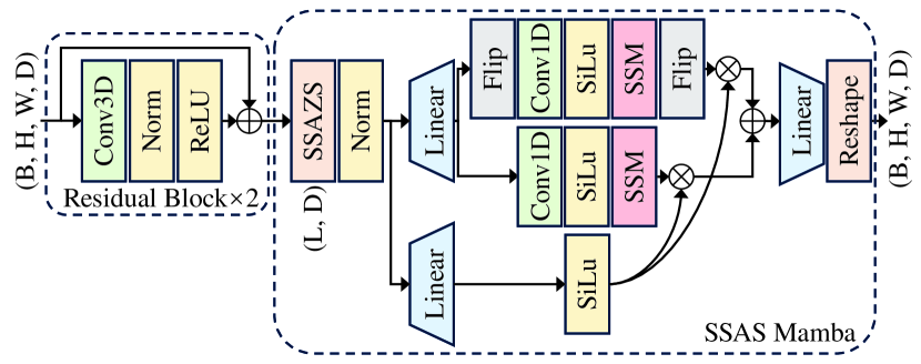
The Mamba model [14] shows compelling characteristics in achieving global receptive fields, dynamic weights, and linear computational complexity. While the sequential nature of Mamba fits well with NLP tasks involving temporal data, it presents significant challenges when applied to HSI data, which is non-sequential and has strong spatial continuity and spectral correlation. To address this issue, we introduce a Spatial-Spectral Alternating Zigzag Scan (SSAZS) Mamba block for HSI modeling. As shown in Fig. 3, the SSAZS Mamba block consists of Residual Blocks and a SSAZS Mamba layer.

Unlike the sequence data, vision data is rich in spatial information [48]. Additionally, HSIs feature strong local spatial-spectral correlation. In our SSAZS Mamba Block, residual blocks with 3-D convolution, Instance Normalization, and Leaky ReLU are applied to the feature to model the local spatial-spectral correlation to enhance the local texture exploration in the SSAZS Mama block.

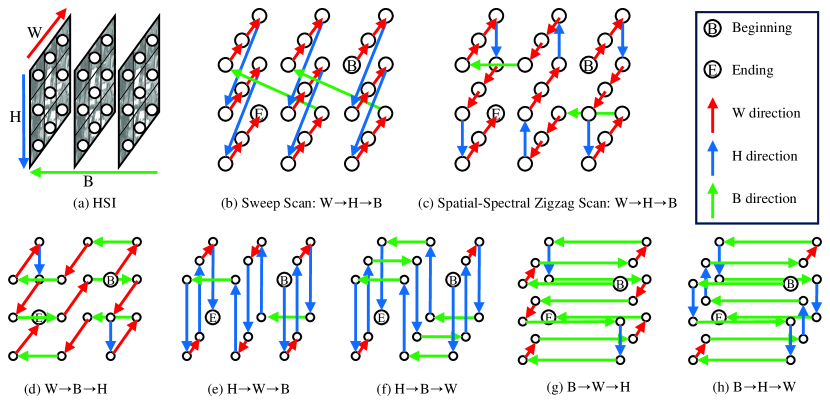
Nevertheless, the SSM models all tokens sequentially. Most current vision SSM-based models lack consideration for spatial continuity in the scan scheme [19, 16, 18]. As shown in Fig. 4(b), the sequence scanning in Mamba defaults to a sweep scan when moving to scan the next line or band, resulting in significant gaps between sequence connections. To address these discontinuities in the scan scheme, we introduce the spatial-spectral zigzag scan in HSI denoising to enhance the continuity of information flow in the SSM. As depicted in Fig. 4(c), we scan the 3-D data of HSI in a zigzag pattern, which allows the SSM to explore a more continuity spatial-spectral information flow.

Moreover, in non-sequential vision data, the correlation among pixels is in more directions [48, 16]. For example, in vision data, a 2-D selective scan [16] is proposed to exploit the 2-D image in 4 directions: H forward scan, H backward scan, W forward scan, and W backward scan. Given that HSIs are 3-D data characterized by strong spatial continuity and spectral correlation, we anticipate information flows in both spatial and spectral dimensions to capture global spatial-spectral correlation. Consequently, we extend the spatial-spectral zigzag scan to a Spatial-Spectral Alternating Zigzag Scan (SSAZS) strategy to thoroughly exploit the information flow in all directions. The SSAZS includes 6 variants with different scanning patterns, illustrated in Fig. 4 (c-h): $\text{W}\rightarrow\text{H}\rightarrow\text{B}$, $\text{W}\rightarrow\text{B}\rightarrow\text{H}$, $\text{H}\rightarrow\text{W}\rightarrow\text{B}$, $\text{H}\rightarrow\text{B}\rightarrow\text{W}$, $\text{B}\rightarrow\text{W}\rightarrow\text{H}$, and $\text{B}\rightarrow\text{H}\rightarrow\text{W}$, where B, H, and W represent the band, height, and width of the HSI, respectively. The first 4 variants will pay attention to the information in the spatial dimension, while the last two variants focus on spectral correlation. We incorporate one of the variants of SSAZS after the residual blocks and flatten the input HSI feature with the shape of (B, H, W, D) into (L, D), where $\text{L}=\text{B}\times\text{H}\times\text{W}$, to make the block scan in a specific pattern. In our SSUMamba, we use 6 SSAZS Mamba blocks with all the 6 variants of SSAZS to accomplish the modeling in all directions in HSIs.

Thanks to SSAZS, Mamba blocks can effectively model information flow in various patterns to capture the 3-D characteristics of HSI. However, these information flows typically proceed sequentially from the beginning point to the ending point. To enhance information flow, we introduce a bidirectional Mamba layer. The features from SSAZS are divided into two parts: one processed in the forward direction and the other in the backward direction. Following the bidirectional Mamba layer, SSAZS achieves comprehensive modeling of global spatial-spectral correlation.

III-D Architecture Design Details

In the standard setting of our SSUMamba, we incorporate 6 SSAZS Mamba blocks with channel set as [32, 64, 64, 128, 128, 256]. The downsampling is enabled in block [2, 4, 6]. The SSUMamba is trained end-to-end to minimize the difference between the predicted clean HSI and the ground truth clean HSI. The loss function is set as:

$$\mathcal{L}=\frac{1}{N}\sum_{i=1}^{N}\|\widehat{\mathcal{Y}}_{i}-\mathcal{Y}_{i}\|_{F}^{2}$$ (7)

where $\mathcal{Y}$ denotes the HSI recovered from the noisy image $\mathcal{X}$ in SSUMamba, $\widehat{\mathcal{Y}}$ denotes the corresponding clean image, and $N$ is the batch size within each iteration. An Adm optimizer with a learning rate of $3\times 10^{-4}$ was used to train the SSUMamba model for 45 epochs and decreased with a factor of 0.5 in the 20th and 35th epochs. The batch size is set as 14. The model was implemented using PyTorch and trained on a single NVIDIA GeForce RTX 3090 GPU.

TABLE I: Comparison of Different Methods on 50 Testing HSIs from ICVL Dataset. The Top Three Values Are Marked as Red, Blue, and Green.

			Model-based methods								Deep learning-based methods
$\sigma$	Index	Noisy	BM4D	MTSNMF	LLRT	NGMeet	LRMR	FastHyDe	LRTF$L_{0}$	E-3DTV	T3SC	MAC-Net	TRQ3D	SST	SSUMamba
			[26]	[22]	[27]	[28]	[21]	[29]	[23]	[30]	[32]	[31]	[13]	[9]	(ours)
[0,15]	PSNR$\uparrow$	33.18	44.39	45.39	45.74	39.63	41.50	48.08	43.41	46.05	49.68	48.21	46.43	50.87	51.34
	SSIM$\uparrow$	.6168	.9683	.9592	.9657	.8612	.9356	.9917	.9315	.9811	.9912	.9915	.9878	.9938	.9946
	SAM$\downarrow$	.3368	.0692	.0845	.0832	.2144	.1289	.0404	.0570	.0560	.0486	.0387	.0437	.0298	.0256
[0,55]	PSNR$\uparrow$	21.72	37.63	38.02	36.80	31.53	31.50	42.86	35.63	40.20	45.15	43.74	44.64	46.39	46.85
	SSIM$\uparrow$	.2339	.9008	.8586	.8285	.6785	.6233	.9800	.8125	.9505	.9810	.9768	.9840	.9872	.9882
	SAM$\downarrow$	.7012	.1397	.234	.2316	.4787	.3583	.0630	.1914	.0993	.0652	.0582	.0487	.0457	.0375
[0,95]	PSNR$\uparrow$	17.43	34.71	34.81	31.89	27.62	27.00	40.84	32.83	37.80	43.10	41.24	43.54	44.83	45.36
	SSIM$\uparrow$	.1540	.8402	.7997	.6885	.5363	.4208	.9734	.7482	.9279	.9734	.9577	.9806	.9838	.9853
	SAM$\downarrow$	.8893	.1906	.3266	.3444	.642	.5142	.0771	.3014	.1317	.0747	.0841	.0523	.0513	.0439
Mixture	PSNR$\uparrow$	13.21	23.36	27.55	18.23	23.61	23.10	27.58	30.93	34.90	34.09	28.44	39.73	39.22	43.07
	SSIM$\uparrow$	.0841	.4275	.6743	.1731	.4448	.3463	.7250	.8378	.9041	.9052	.7393	.9491	.9626	.9726
	SAM$\downarrow$	.9124	.5476	.5326	.6873	.6252	.5144	.4534	.3613	.1468	.2340	.4154	.0869	.0743	.0710

IV Experiments

In this section, we demonstrate the denoising performance of the proposed SSUMamba through synthetic and real-world experiments. Additionally, we conduct further ablation experiments to analyze the performance of each module and varying widths within the network.

IV-A Experimental Settings

IV-A1 Training and Testing Setting

In accordance with [11, 31], we opted for 100 HSIs from the Interdisciplinary Computational Vision Laboratory (ICVL) HSI dataset for training. These HSIs were captured using a Specim PS Kappa DX4 hyperspectral camera, sized at $1392\times 1300$ pixels and covering 31 spectral bands ranging from 400 to 700 nm. They were partitioned into patches measuring $64\times 64\times 31$ and subjected to augmentation through random flipping, cropping, and resizing. The synthetic datasets include the ICVL testing set, Houston 2018 HSI, and Pavia City Center HSI. The real-world datasets comprise the Gaofen-5 (GF-5) Wuhan HSI and the Earth Observing-1 (EO-1) HSI. The number of bands also increases from ICVL to EO-1 HSI, providing a comprehensive evaluation set to test all methods across varying numbers of bands and spectrum characteristics.

IV-A2 Synthetic Data Generation

As indicated by  [53], real-world noises in hyperspectral images (HSIs) typically follow non-independent and identical distribution (non-i.i.d.). Furthermore, remote-sensing HSIs commonly exhibit contamination from a mixture of noises. Hence, in our experiments, we considered non-i.i.d. Gaussian noise and mixture noise. For non-i.i.d. Gaussian noise, we varied the standard deviation within the range of $\sigma\in$ [0, 15], [0, 55], and [0, 95]. The mixture noise comprised the following components: 1) non-i.i.d. Gaussian noise with $\sigma\in$ [0, 95]; 2) impulse noise affecting 1/3 of the bands, with intensities spanning from 10% to 70%; 3) strips affecting 5%-15% of columns on 1/3 of the bands; and 4) dead zones affecting 5%-15% of columns on 1/3 of the bands.

IV-A3 Evaluation Index

To quantitatively assess the denoising performance of all methods, we employed peak signal-to-noise ratio (PSNR), structural similarity (SSIM), and spectral angle mapper (SAM). Higher PSNR and SSIM values, along with smaller SAM values, indicate superior denoising effectiveness.

IV-A4 Comparison Methods

12 methods were used for comparison, including 8 model-based methods, i.e., BM4D [26], MTSNMF [22], LLRT [27], NGMeet [28], LRMR [21], FastHyDe [29], LRTF$L_{0}$ [23], and E-3DTV [30], and 4 deep learning-based methods, i.e., T3SC [32], MAC-Net [31], TRQ3D [13], and SST [9]. For a fair comparison, we retrained one model for all the deep learning-based methods in each noise case.

IV-B Comparison on Synthetic Datasets

To demonstrate the denoising performance both quantitatively and qualitatively, we first present the denoising results on the ICVL testing set, Houston 2018 HSI, and Pavia City Center HSI.

IV-B1 ICVL testing set

The ICVL dataset comprises 50 HSIs from the ICVL dataset for synthetic testing. To alleviate the computational burden associated with certain model-based techniques like NGMeet, all these HSIs were resized to $512\times 512\times 31$. The ICVL dataset is enriched with a greater number of HSIs, offering a comprehensive evaluation platform to assess the performance of all methods under different noise cases. Thus, both Gaussian and mixture noises were included for assessment. Table I illustrates the quantitative analysis, with the top three results highlighted in bold red, bold blue, and bold green, respectively.

FastHyDe demonstrates superior performance among model-based methods in Gaussian noise cases, attributed to its simultaneous modeling of the GSC and NSS of HSIs. For mixture noise cases, methods like LRTF$L_{0}$ and E-3DTV exhibit improved performance. Deep learning-based approaches leverage their data-driven learning capability, outperforming model-based methods consistently. T3SC and MAC-Net leverage physical modeling and data-driven learning, showcasing robustness against Gaussian noise. Constrained with spectral and spatial transformer-based modules, SST shows the best performance among all comparison methods. In summary, SSUMamba stands out as the top performance in all assessed cases. This is attributed to its capability to adeptly capture the domain knowledge of HSIs through global spatial-spectral correlation modeling.

IV-B2 Houston 2018 HSI

TABLE II: Comparison of Different Methods on Houston 2018 HSI. The Top Three Values Are Marked as Red, Blue, and Green.

		Model-based methods								Deep learning-based methods
Index	Noisy	BM4D	MTSNMF	LLRT	NGMeet	LRMR	FastHyDe	LRTF$L_{0}$	E-3DTV	T3SC	MAC-Net	TRQ3D	SST	SSUMamba
		[26]	[22]	[27]	[28]	[21]	[29]	[23]	[30]	[32]	[31]	[13]	[9]	(ours)
PSNR$\uparrow$	11.72	22.76	25.86	15.58	22.36	21.84	27.07	28.75	30.64	29.84	28.83	32.55	31.07	34.74
SSIM$\uparrow$	.0843	.4762	.6933	.1386	.5169	.3914	.7757	.8038	.8570	.8751	.7963	.9194	.9166	.9452
SAM$\downarrow$	.9778	.5168	.4977	.7652	.5728	.4857	.4518	.2221	.1323	.1943	.2356	.1241	.1390	.0993

(a) Clean

(b) Noisy

(c) BM4D [26]

(d) MTSNMF [22]

(e) LLRT [27]

(f) NGMeet [28]

(g) LRMR [21]

(h) FastHyDe [29]

(i) LRTF$L_{0}$ [23]

(j) E-3DTV [30]

(k) T3SC [32]

(l) MAC-Net [31]

(m) TRQ3D [13]

(n) SST [9]

(o) SSUMamba

Figure 5: Denoising results on the Houston 2018 HSI with the mixture noise. The false-color images are generated by combining bands 35, 20, and 5.

(a) Clean

(b) Noisy

(c) BM4D [26]

(d) MTSNMF [22]

(e) LLRT [27]

(f) NGMeet [28]

(g) LRMR [21]

(h) FastHyDe [29]

(i) LRTF$L_{0}$ [23]

(j) E-3DTV [30]

(k) T3SC [32]

(l) MAC-Net [31]

(m) TRQ3D [13]

(n) SST [9]

(o) SSUMamba

Figure 6: Reflectance of pixel (374,182) in the Houston 2018 HSI.

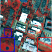
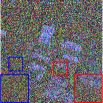
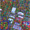
The Houston 2018 HSI was captured using the ITRES CASI hyperspectral imager, comprising $1202\times 4172$ pixels. The Houston HSI contains 48 bands spanning from 380 to 1050 nm. For our experiments, we omit the first 2 bands, which are relatively noisy, and extracted a $512\times 512$ cube from the center of the HSI for synthetic experiments. To replicate real-world noise found in remote-sensing images, we introduced mixture noise to the pristine HSI, resulting in a noisy HSI. Deep learning models trained on the ICVL dataset were then employed for evaluation. However, it is noteworthy that T3SC, TRQ3D, and SST encounter challenges when dealing with HSIs that feature a distinct number of bands compared to the training data. To mitigate this issue, for T3SC, TRQ3D, and SST, we partitioned the provided HSI into multiple sub-images, each containing 31 bands for testing.

The denoising results are showcased in Table II. All deep learning-based methods learn the mixture noise cases in the ICVL dataset and perform better than model-based methods. However, given the substantial divergence between the Houston 2018 HSI and the training set ICVL, deep learning-based techniques face a formidable challenge when tasked with denoising and exhibiting a decline in performance. Our proposed SSUMamba, despite experiencing some performance degradation in instances of significant data discrepancies, still outperforms transformer-based approaches.

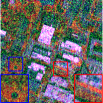
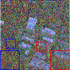
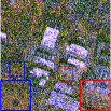
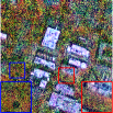
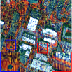
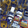
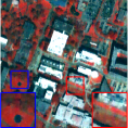
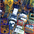
Fig. 5 illustrates the false-color images recovered from all comparison methods. While conventional model-based approaches, tailored for Gaussian noise, struggle with eliminating artifacts such as stripes and artifacts, E-3DTV stands out by employing the $l1$-norm for noise in the mixture noise. Due to spectral variations between the Houston HSI and the ICVL training set, TRQ3D and SST transformers exhibit some degree of failure in Houston image reconstruction. TRQ3D retaining Gaussian noise and stripe artifacts. SST exhibits color distortion, indicating inaccuracies in spectral fidelity relative to the original image, thus revealing limitations in accurately modeling spectral correlations. In contrast, our SSUMamba model utilizes alternating scan Mamba blocks to capture global spatial-spectral correlations effectively. Our method yields highly accurate reconstructions with minimal artifacts, particularly in cases with mixture noise, where detailed information degrades. Exploiting long-range spatial-spectral information can help recover degraded data and substantially improve overall performance.

The spectral reflectances are shown in Fig. 6, where the mixture noise makes the spectral distortion drastic, as in Fig. 6(b). Because model-based methods are susceptible to noise type, they struggle to generate recovered spectra that match clean image spectra in denoising mixture noise. Taking into account the mixed noise, E-3DTV models the low-rankness of the spatial and spectral gradient map in HSI, resulting in the best match with the clean HSI among model-based methods. Deep learning-based T3SC and E-3DTV design for Gaussian noise recover the spectral reflectance with jitters. TRQ3D and SST cannot accommodate the processing as the number of bands in Houston 2018 differs from that in the ICVL training set, resulting in incomplete GSC and less accurate matching of spectral reflectances with clean HSI. Our SSUMamba, with the ability to capture global spatial-spectral correlations, can effectively recover spectral reflectance, demonstrating the best performance in spectral modeling ability among all methods.

IV-B3 Pavia City Center HSI

TABLE III: Comparison of Different Methods on Pavia City Center HSI. The Top Three Values Are Marked as Red, Blue, and Green.

		Model-based methods								Deep learning-based methods
Index	Noisy	BM4D	MTSNMF	LLRT	NGMeet	LRMR	FastHyDe	LRTF$L_{0}$	E-3DTV	T3SC	MAC-Net	TRQ3D	SST	SSUMamba
		[26]	[22]	[27]	[28]	[21]	[29]	[23]	[30]	[32]	[31]	[13]	[9]	(ours)
PSNR$\uparrow$	13.46	21.70	25.15	15.44	23.68	22.72	26.78	26.49	30.44	28.69	27.74	28.23	31.87	35.70
SSIM$\uparrow$	.2181	.5128	.7397	.2760	.7176	.6524	.8361	.8147	.8941	.8656	.8724	.8665	.9234	.9546
SAM$\downarrow$	.8893	.5297	.4094	.7902	.4760	.3771	.4040	.3703	.1134	.2135	.3222	.1961	.1676	.1057

(a) Clean

(b) Noisy

(c) BM4D [26]

(d) MTSNMF [22]

(e) LLRT [27]

(f) NGMeet [28]

(g) LRMR [21]

(h) FastHyDe [29]

(i) LRTF$L_{0}$ [23]

(j) E-3DTV [30]

(k) T3SC [32]

(l) MAC-Net [31]

(m) TRQ3D [13]

(n) SST [9]

(o) SSRT-UNet

Figure 7: Denoising results on the Pavia City Center HSI with the mixture noise. The false-color images are generated by combining bands 65, 45, and 25.

(a) Clean

(b) Noisy

(c) BM4D [26]

(d) MTSNMF [22]

(e) LLRT [27]

(f) NGMeet [28]

(g) LRMR [21]

(h) FastHyDe [29]

(i) LRTF$L_{0}$ [23]

(j) E-3DTV [30]

(k) T3SC [32]

(l) MAC-Net [31]

(m) TRQ3D [13]

(n) SST [9]

(o) SSRT-UNet

Figure 8: Reflectance of pixel (170,100) in the Pavia City Center HSI.

The Pavia City Center HSI was captured using the Reflective Optics System Imaging Spectrometer (ROSIS) sensor spanning from 430 to 860 nm. Following [54], we removed the first 22 noisy bands and added mixture noise on a $200\times 200$ subimage with 80 bands for synthetic experiments. Other experimental settings were maintained in line with those used for the Houston 2018 HSI.

Table III shows a quantitative presentation of the results of the experiment. Model-based E-3DTV calculates sparsity on gradient map subspaces across all HSI bands. Its ability to better reflect spectral correlations and differences allows E-3DTV to outperform TRQ3D, which introduces RNNs to model incomplete spectral correlations in the HSI, especially when the Pavia City Center HSI has different spectral features from the training data. Exploiting long-range correlations in spectral and spatial dimensions, transformer-based SST shows better performance than TRQ3D. However, it still struggles when dealing with testing data with a different number of bands. Our SSUMamba achieves the best performance in the Pavia City Center HSI by exploiting complete global spatial-spectral correlations with SSM.

(a) Original

(b) BM4D [26]

(c) MTSNMF [22]

(d) LLRT [27]

(e) NGMeet [28]

(f) LRMR [21]

(g) FastHyDe [29]

(h) LRTF$L_{0}$ [23]

(i) E-3DTV [30]

(j) T3SC [32]

(k) MAC-Net [31]

(l) TRQ3D [13]

(m) SST [9]

(n) SSRT-UNet

Figure 9: Denoising results on the GF-5 Wuhan HSI. The false-color images are generated by combining bands 152, 83, and 33.

(a) Original

(b) BM4D [26]

(c) MTSNMF [22]

(d) LLRT [27]

(e) NGMeet [28]

(f) LRMR [21]

(g) FastHyDe [29]

(h) LRTF$L_{0}$ [23]

(i) E-3DTV [30]

(j) T3SC [32]

(k) MAC-Net [31]

(l) TRQ3D [13]

(m) SST [9]

(n) SSRT-UNet

Figure 10: Reflectance of pixel (248,273) in the GF-5 Wuhan HSI.

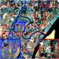
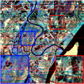
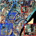
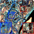
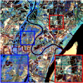
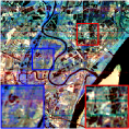
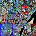
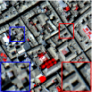
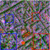
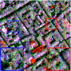
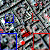
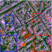
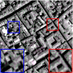
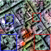
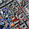
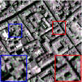
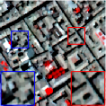
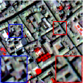
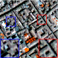
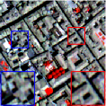
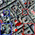
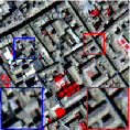
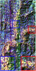
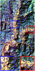
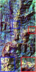
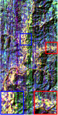
Fig. 7 shows the false-color images recovered by all comparison methods. The model-based methods, designed for Gaussian noise, fail to eliminate artifacts such as stripes and artifacts in the mixture noise. E-3DTV, which models the low-rankness of the spatial and spectral gradient map in HSI, achieves the best performance in the mixture noise. However, it still gets blurred due to the limited ability of spatial correlation modeling. Transformer-based methods, such as TRQ3D and SST, exhibit some degree of failure in reconstruction due to spectral variations between the Pavia City Center HSI and the training set ICVL. Our SSUMamba, which captures global spatial-spectral correlations effectively, yields highly accurate reconstructions with minimal artifacts, particularly in cases with heavy noise, where detailed information degrades. Fig. 8 shows the spectral reflectances of the mixture noise. The proposed SSUMamba effectively exploits global spatial-spectral correlations to recover spectral reflectance, resulting in the best match with the clean HSI among all methods.

(a) Original

(b) BM4D [26]

(c) MTSNMF [22]

(d) LLRT [27]

(e) NGMeet [28]

(f) LRMR [21]

(g) FastHyDe [29]

(h) LRTF$L_{0}$ [23]

(i) E-3DTV [30]

(j) T3SC [32]

(k) MAC-Net [31]

(l) TRQ3D [13]

(m) SST [9]

(n) SSRT-UNet

Figure 11: Denoising results on the EO-1 HSI. The false-color images are generated by combining bands 163, 96, and 30.

(a) Original

(b) BM4D [26]

(c) MTSNMF [22]

(d) LLRT [27]

(e) NGMeet [28]

(f) LRMR [21]

(g) FastHyDe [29]

(h) LRTF$L_{0}$ [23]

(i) E-3DTV [30]

(j) T3SC [32]

(k) MAC-Net [31]

(l) TRQ3D [13]

(m) SST [9]

(n) SSRT-UNet

Figure 12: Reflectance of pixel (151,125) in the EO-1 HSI.

IV-C Comparison on Real-World HSIs

We carried out extra experiments on real-world remote-sensing HSIs to thoroughly evaluate the effectiveness of denoising across various methods. We provide a qualitative comparative analysis to assess the denoising results.

IV-C1 Gaofen-5 Wuhan HSI

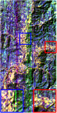
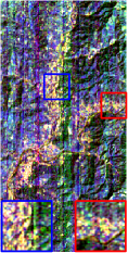
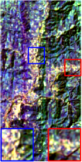
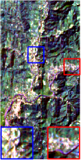
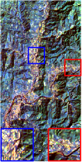
The Gaofen-5 (GF-5) Wuhan HSI was acquired using the Advanced Hyperspectral Imager (AHSI) with a resolution of $300\times 300$ pixels and 155 spectral bands. In our real-world experiment, we applied all comparison methods to the original noisy HSI. The results are presented in Fig. 9, where the original image is degraded by impulse and stripes. Among model-based methods, FastHyDe and LRTF$L_{0}$ achieved better performance thanks to their ability to recover from mixture noise. T3SC and MAC-Net effectively removed most of the stripes in the GF-5 Wuhan HSI. T3SC produced sharper results by learning both spectral and spatial information in a trainable sparse coding model. However, Transformer-based TRQ3D and SST failed to completely remove all the stripes due to limited adaptability to the imaging environment. Our SSUMamba method, which effectively captures global spatial-spectral correlations to learn the deep 3-D features of the HSI, yielded highly accurate reconstructions with minimal artifacts and sharper edges compared to all other methods.

Spectral reflectances are depicted in Fig. 10. The heavy impulse and stripes cause significant spectral distortion, as seen in Fig. 10(a). T3SC and SST process the HSI in patches, leading to incomplete global spatial-spectral correlations and spectral jitters. In contrast, our SSUMamba, which captures global spatial-spectral correlations effectively, can recover spectral reflectance more accurately, resulting in smoother curves that closely resemble the original shape.

IV-C2 Earth Observing-1 HSI

The Earth Observing-1 (EO-1) HSI was acquired by Hyperion with 242 bands and a resolution of $1000\times 400$ pixels. Following [21], the water absorption bands were removed, and the final HSI was cropped to $400\times 200$ pixels with 166 bands. Similar to the experiment with the GF-5 Wuhan HSI, we applied all comparison methods to the original noisy HSI. The results are presented in Fig. 11. The presence of heavier impulse and stripe noise makes the denoising task more challenging. Besides E-3DTV, all other model-based methods failed to effectively remove the stripes and impulse noise due to the heavier noise. Although E-3DTV removed the stripes and impulse noise, it resulted in blurred edges. Among deep learning-based methods, T3SC and TRQ3D successfully removed most of the stripes. However, insufficient modeling of global spatial-spectral correlations resulted in blurring similar to E-3DTV. MAC-Net and SST were unable to remove all the stripes, while SST introduced color distortion. Our SSUMamba effectively learned the deep 3-D nature of the HSI, incorporating spatial and spectral information to produce sharper edges and more accurate colors. Spectral reflectances are shown in Fig. 12, where jitters and discontinuities are evident in Fig. 12(a). SSUMamba achieved smoother and more continuous spectral reflectance.

IV-D Ablation Study

In this section, we present the performance of SSUMamba on different modules to demonstrate their individual contributions to performance. Additionally, we evaluate the impact of network width on the performance of SSUMamba.

IV-D1 Effectiveness of Different Modules

We assess the efficacy of the components introduced in SSUMamba, which include the spatial-spectral zigzag scan, alternating strategy, and bidirectional Mamba. The model was trained on the ICVL training set and tested on the ICVL testing set, Houston 2018 HSI, and Pavia City Center HSI with mixed noise. The results are presented in Table IV. The zigzag scan allows the SSM to scan the HSI in a zigzag pattern, which effectively enhances the continuity of the spatial-spectral information flow. The bidirectional Mamba allows the network to scan the HSI in both forward and backward directions, further refining the multidirectional modeling. The bidirectional Mamba allows the network to scan the HSI in both forward and backward directions, which further refines the multi-directional modeling. Incorporating the zigzag scan and alternating strategy does not introduce additional parameters or computational complexity; rather, it aids the model in exploiting information flows in the 3-D nature of the HSI data in all directions. In summary, the network with Spatial-Spectral Alternating Zigzag Scan (SSAZS) has the optimal performance. Furthermore, the introduction of the bidirectional Mamba further refines the global spatial-spectral correlation modeling, resulting in enhanced performance across all cases.

TABLE IV: Ablation Study on The Effect of Introduced Components.

Zigzag	Alternating	Bidirectional	ICVL			Houston 2018 HSI			Pavia City Center HSI
			PSNR$\uparrow$	SSIM$\uparrow$	SAM$\downarrow$	PSNR$\uparrow$	SSIM$\uparrow$	SAM$\downarrow$	PSNR$\uparrow$	SSIM$\uparrow$	SAM$\downarrow$
✓	✓	✓	43.07	.9726	.0710	34.74	.9452	.0993	35.70	.9546	.1057
✗	✓	✓	42.76	.9701	.0710	34.55	.9444	.1047	35.58	.9557	.1055
✗	✗	✓	42.73	.9710	.0689	34.40	.9444	.1056	35.76	.9507	.1036
✓	✓	✗	42.74	.9701	.0672	34.51	.9435	.1051	35.63	.9528	.1139

TABLE V: Ablation Study on The Impact of Network Width (Channels).

Channels	#Param.	Memory	ICVL			Houston 2018 HSI			Pavia City Center HSI
			PSNR$\uparrow$	SSIM$\uparrow$	SAM$\downarrow$	PSNR$\uparrow$	SSIM$\uparrow$	SAM$\downarrow$	PSNR$\uparrow$	SSIM$\uparrow$	SAM$\downarrow$
32	10.4M	1,802M	43.07	.9726	.0710	34.74	.9452	.0993	35.70	.9546	.1057
24	5.9M	1,386M	42.67	.9711	.0675	33.96	.9374	.1074	34.09	.9440	.1284
16	2.6M	991M	41.34	.9659	.0694	33.80	.9365	.1095	33.63	.9397	.1210
8	0.68M	585M	40.50	.9645	.0725	31.27	.8982	.1516	28.85	.8815	.1839
Methods	#Param.	Memory	ICVL			Houston 2018 HSI			Pavia City Center HSI
			PSNR$\uparrow$	SSIM$\uparrow$	SAM$\downarrow$	PSNR$\uparrow$	SSIM$\uparrow$	SAM$\downarrow$	PSNR$\uparrow$	SSIM$\uparrow$	SAM$\downarrow$
TRQ3D	0.68M	675M	39.73	.9491	.0869	32.55	.9194	.1241	28.23	.8665	.1961
SST	4.1M	1,600M	39.22	.9626	.0743	31.07	.9166	.1390	31.87	.9234	.1676

IV-D2 Impact of Width

We further investigate the effectiveness of network width in our SSUMamba framework. To assess the impact of network width on performance, we conducted experiments with varying numbers of channels, which play a pivotal role in the network width. In the 6 SSAZS Mamba blocks, the channel configuration is set as [$BC,BC\times 2,BC\times 2,BC\times 4,BC\times 4,BC\times 8$], where $BC$ means base channels. We compare the performance of SSUMamba with different numbers of base channels, including 32, 24, 16, and 8. We also compare the results with transformer-based methods, TRQ3D and SST. All networks were trained on the ICVL training set and tested on all synthetic datasets with mixed noise. The results are presented in Table V, where we show the number of parameters and memory consumption per batch in training for networks of different widths. As we can see, the performance of our proposed SSUMamba continues to extend as the width is enhanced. Compared with transformer-based methods, which suffer from the $\text{O}(n^{2})$ complexity, our SSUMamba achieves better performance with fewer parameters and lower memory consumption. This is achieved thanks to the linear complexity facilitated by SSM and global spatial-spectral correlation modeling in our SSAZS Mamba block.

V Conclusion

This paper introduces a SSUMamba for HSI denoising. We incorporate the SSM with linear complexity to enable global spatial-spectral correlation modeling in HSIs. By utilizing the Spatial-Spectral Alternating Zigzag Scan Mamba block, our SSUMamba can effectively exploit the information flow in all directions in the HSI data and enhance the 3-D characteristic. Experimental results with comparison methods demonstrate that our proposed method achieves state-of-the-art performance. The ablation study further validates the effectiveness of the introduced components.

References

- [1] B. Thai and G. Healey, “Invariant subpixel material detection in hyperspectral imagery,” IEEE Trans. Geosci. Remote Sens., vol. 40, no. 3, pp. 599–608, 2002.
- [2] X. Yang, B. Tu, Q. Li, J. Li, and A. Plaza, “Graph evolution-based vertex extraction for hyperspectral anomaly detection,” IEEE Trans. Neural Netw. Learn. Syst., pp. 1–15, 2023.
- [3] L. Gao, X. Sun, X. Sun, L. Zhuang, Q. Du, and B. Zhang, “Hyperspectral anomaly detection based on chessboard topology,” IEEE Trans. Geosci. Remote Sens., vol. 61, pp. 1–16, 2023.
- [4] W. Dong, J. Zhao, J. Qu, S. Xiao, N. Li, S. Hou, and Y. Li, “Abundance matrix correlation analysis network based on hierarchical multihead self-cross-hybrid attention for hyperspectral change detection,” IEEE Trans Geosci Remote Sens, vol. 61, pp. 1–13, 2023.
- [5] F. Xiong, J. Zhou, and Y. Qian, “Material based object tracking in hyperspectral videos,” IEEE Trans. Image Process., vol. 29, pp. 3719–3733, 2020.
- [6] Z. Li, F. Xiong, J. Zhou, J. Lu, and Y. Qian, “Learning a deep ensemble network with band importance for hyperspectral object tracking,” IEEE Trans. Image Process., vol. 32, pp. 2901–2914, 2023.
- [7] F. Luo, T. Zhou, J. Liu, T. Guo, X. Gong, and J. Ren, “Multiscale diff-changed feature fusion network for hyperspectral image change detection,” IEEE Trans. Geosci. Remote Sens., vol. 61, pp. 1–13, 2023.
- [8] N. Li, S. Jiang, J. Xue, S. Ye, and S. Jia, “Texture-aware self-attention model for hyperspectral tree species classification,” IEEE Trans. Geosci. Remote Sens., vol. 62, pp. 1–15, 2024.
- [9] M. Li, Y. Fu, and Y. Zhang, “Spatial-spectral transformer for hyperspectral image denoising,” in Proc. AAAI Conf. Artif. Intell. (AAAI), 2023.
- [10] G. Fu, F. Xiong, J. Lu, J. Zhou, J. Zhou, and Y. Qian, “Hyperspectral image denoising via spatial–spectral recurrent transformer,” IEEE Trans. Geosci. Remote Sens., vol. 62, pp. 1–14, 2024.
- [11] K. Wei, Y. Fu, and H. Huang, “3-D quasi-recurrent neural network for hyperspectral image denoising,” IEEE Trans. Neural Netw. Learn. Syst., vol. 32, no. 1, pp. 363–375, 2021.
- [12] X. Fu, Y. Guo, M. Xu, and S. Jia, “Hyperspectral image denoising via robust subspace estimation and group sparsity constraint,” IEEE Trans. Geosci. Remote Sens., vol. 61, pp. 1–16, 2023.
- [13] L. Pang, W. Gu, and X. Cao, “TRQ3DNet: A 3D quasi-recurrent and transformer based network for hyperspectral image denoising,” Remote Sensing, vol. 14, no. 18, 2022.
- [14] A. Gu and T. Dao, “Mamba: Linear-time sequence modeling with selective state spaces,” arXiv preprint arXiv:2312.00752, 2023.
- [15] A. Gu, K. Goel, and C. Re, “Efficiently modeling long sequences with structured state spaces,” in Proc. Int. Conf. Learn. Represent. (ICLR), 2022.
- [16] Y. Liu, Y. Tian, Y. Zhao, H. Yu, L. Xie, Y. Wang, Q. Ye, and Y. Liu, “Vmamba: Visual state space model,” arXiv preprint arXiv:2401.10166, 2024.
- [17] K. Li, X. Li, Y. Wang, Y. He, Y. Wang, L. Wang, and Y. Qiao, “Videomamba: State space model for efficient video understanding,” arXiv preprint arXiv:2403.06977, 2024.
- [18] L. Zhu, B. Liao, Q. Zhang, X. Wang, W. Liu, and X. Wang, “Vision mamba: Efficient visual representation learning with bidirectional state space model,” arXiv preprint arXiv:2401.09417, 2024.
- [19] V. T. Hu, S. A. Baumann, M. Gui, O. Grebenkova, P. Ma, J. Fischer, and B. Ommer, “Zigma: Zigzag mamba diffusion model,” arXiv preprint arXiv:2403.13802, 2024.
- [20] Y. Liu, J. Xiao, Y. Guo, P. Jiang, H. Yang, and F. Wang, “Hsidmamba: Exploring bidirectional state-space models for hyperspectral denoising,” arXiv preprint arXiv:2404.09697, 2024.
- [21] H. Zhang, W. He, L. Zhang, H. Shen, and Q. Yuan, “Hyperspectral image restoration using low-rank matrix recovery,” IEEE Trans. Geosci. Remote Sens., vol. 52, no. 8, pp. 4729–4743, 2014.
- [22] M. Ye, Y. Qian, and J. Zhou, “Multitask sparse nonnegative matrix factorization for joint spectral–spatial hyperspectral imagery denoising,” IEEE Trans. Geosci. Remote Sens., vol. 53, no. 5, pp. 2621–2639, 2014.
- [23] F. Xiong, J. Zhou, and Y. Qian, “Hyperspectral restoration via gradient regularized low-rank tensor factorization,” IEEE Trans. Geosci. Remote Sens., vol. 57, no. 12, pp. 10 410–10 425, 2019.
- [24] Z. Zha, B. Wen, X. Yuan, J. Zhang, J. Zhou, Y. Lu, and C. Zhu, “Nonlocal structured sparsity regularization modeling for hyperspectral image denoising,” IEEE Trans. Geosci. Remote Sens., vol. 61, pp. 1–16, 2023.
- [25] X. Su, Z. Zhang, and F. Yang, “Fast hyperspectral image denoising and destriping method based on graph laplacian regularization,” IEEE Trans. Geosci. Remote Sens., vol. 61, pp. 1–14, 2023.
- [26] M. Maggioni, V. Katkovnik, K. Egiazarian, and A. Foi, “Nonlocal transform-domain filter for volumetric data denoising and reconstruction,” IEEE Trans. Image Process., vol. 22, no. 1, pp. 119–133, 2012.
- [27] Y. Chang, L. Yan, and S. Zhong, “Hyper-Laplacian regularized unidirectional low-rank tensor recovery for multispectral image denoising,” in Proc. IEEE Conf. Comput. Vis. Pattern Recognit. (CVPR), 2017, pp. 5901–5909.
- [28] W. He, Q. Yao, C. Li, N. Yokoya, Q. Zhao, H. Zhang, and L. Zhang, “Non-local meets global: An iterative paradigm for hyperspectral image restoration,” IEEE Trans. Pattern Anal. Mach. Intell., vol. 44, no. 4, pp. 2089–2107, 2022.
- [29] L. Zhuang and J. M. Bioucas-Dias, “Fast hyperspectral image denoising and inpainting based on low-rank and sparse representations,” IEEE J. Sel. Topics Appl. Earth Observations Remote Sens., vol. 11, no. 3, pp. 730–742, 2018.
- [30] J. Peng, Q. Xie, Q. Zhao, Y. Wang, L. Yee, and D. Meng, “Enhanced 3DTV regularization and its applications on HSI denoising and compressed sensing,” IEEE Trans. Image Process., vol. 29, pp. 7889–7903, 2020.
- [31] F. Xiong, J. Zhou, Q. Zhao, J. Lu, and Y. Qian, “MAC-Net: Model-aided nonlocal neural network for hyperspectral image denoising,” IEEE Trans. Geosci. Remote Sens., vol. 60, pp. 1–14, 2022.
- [32] T. Bodrito, A. Zouaoui, J. Chanussot, and J. Mairal, “A trainable spectral-spatial sparse coding model for hyperspectral image restoration,” in Proc. Adv. Neural Inf. Process. Syst. (NeurIPS), vol. 34, 2021, pp. 5430–5442.
- [33] K. Zhang, W. Zuo, Y. Chen, D. Meng, and L. Zhang, “Beyond a Gaussian denoiser: Residual learning of deep CNN for image denoising,” IEEE Trans. Image Process., vol. 26, no. 7, pp. 3142–3155, 2017.
- [34] A. Maffei, J. M. Haut, M. E. Paoletti, J. Plaza, L. Bruzzone, and A. Plaza, “A single model CNN for hyperspectral image denoising,” IEEE Trans. Geosci. Remote Sens., vol. 58, no. 4, pp. 2516–2529, 2020.
- [35] W. Liu and J. Lee, “A 3-D atrous convolution neural network for hyperspectral image denoising,” IEEE Trans. Geosci. Remote Sens., vol. 57, no. 8, pp. 5701–5715, 2019.
- [36] W. Dong, H. Wang, F. Wu, G. Shi, and X. Li, “Deep spatial–spectral representation learning for hyperspectral image denoising,” IEEE Transactions on Computational Imaging, vol. 5, no. 4, pp. 635–648, 2019.
- [37] G. Fu, F. Xiong, J. Lu, J. Zhou, and Y. Qian, “Nonlocal spatial–spectral neural network for hyperspectral image denoising,” IEEE Trans. Geosci. Remote Sens., vol. 60, pp. 1–16, 2022.
- [38] D. Hong, Z. Han, J. Yao, L. Gao, B. Zhang, A. Plaza, and J. Chanussot, “Spectralformer: Rethinking hyperspectral image classification with transformers,” IEEE Trans. Geosci. Remote Sens., vol. 60, pp. 1–15, 2022.
- [39] S. Zhang, J. Zhang, X. Wang, J. Wang, and Z. Wu, “ELS2T: Efficient lightweight spectral-spatial transformer for hyperspectral image classification,” IEEE Trans. Geosci. Remote Sens., 2023.
- [40] H. Yu, Z. Xu, K. Zheng, D. Hong, H. Yang, and M. Song, “MSTNet: A multilevel spectral–spatial transformer network for hyperspectral image classification,” IEEE Trans. Geosci. Remote Sens., vol. 60, pp. 1–13, 2022.
- [41] H. Yang, H. Yu, K. Zheng, J. Hu, T. Tao, and Q. Zhang, “Hyperspectral image classification based on interactive transformer and cnn with multilevel feature fusion network,” IEEE Geosci. Remote Sens. Lett., vol. 20, pp. 1–5, 2023.
- [42] M. Jiang, Y. Su, L. Gao, A. Plaza, X.-L. Zhao, X. Sun, and G. Liu, “GraphGST: Graph generative structure-aware transformer for hyperspectral image classification,” IEEE Trans. Geosci. Remote Sens., vol. 62, pp. 1–16, 2024.
- [43] F. Wang, J. Li, Q. Yuan, and L. Zhang, “Local–global feature-aware transformer based residual network for hyperspectral image denoising,” IEEE Trans. Geosci. Remote Sens., vol. 60, pp. 1–19, 2022.
- [44] M. Li, J. Liu, Y. Fu, Y. Zhang, and D. Dou, “Spectral enhanced rectangle transformer for hyperspectral image denoising,” in Proc. IEEE Conf. Comput. Vis. Pattern Recognit. (CVPR), June 2023, pp. 5805–5814.
- [45] L. Chen, G. Vivone, J. Qin, J. Chanussot, and X. Yang, “Spectral–spatial transformer for hyperspectral image sharpening,” IEEE Trans. Neural Netw. Learn. Syst., 2023.
- [46] Z. Liu, J. Ning, Y. Cao, Y. Wei, Z. Zhang, S. Lin, and H. Hu, “Video swin transformer,” in Proc. IEEE Conf. Comput. Vis. Pattern Recognit. (CVPR), 2022, pp. 3202–3211.
- [47] J. He, L. Zhao, H. Yang, M. Zhang, and W. Li, “HSI-BERT: Hyperspectral image classification using the bidirectional encoder representation from transformers,” IEEE Trans. Geosci. Remote Sens., vol. 58, no. 1, pp. 165–178, 2020.
- [48] G. Chen, Y. Huang, J. Xu, B. Pei, Z. Chen, Z. Li, J. Wang, K. Li, T. Lu, and L. Wang, “Video mamba suite: State space model as a versatile alternative for video understanding,” arXiv preprint arXiv:2403.09626, 2024.
- [49] J. Ma, F. Li, and B. Wang, “U-mamba: Enhancing long-range dependency for biomedical image segmentation,” arXiv preprint arXiv:2401.04722, 2024.
- [50] Y. Shi, B. Xia, X. Jin, X. Wang, T. Zhao, X. Xia, X. Xiao, and W. Yang, “VmambaIR: Visual state space model for image restoration,” arXiv preprint arXiv:2403.11423, 2024.
- [51] J. X. Yang, J. Zhou, J. Wang, H. Tian, and A. W. C. Liew, “Hsimamba: Hyperpsectral imaging efficient feature learning with bidirectional state space for classification,” arXiv preprint arXiv:2404.00272, 2024.
- [52] J. Yao, D. Hong, C. Li, and J. Chanussot, “Spectralmamba: Efficient mamba for hyperspectral image classification,” arXiv preprint arXiv:2404.08489, 2024.
- [53] Y. Chen, X. Cao, Q. Zhao, D. Meng, and Z. Xu, “Denoising hyperspectral image with non-i.i.d. noise structure,” IEEE Trans. Cybern., vol. 48, no. 3, pp. 1054–1066, 2018.
- [54] W. He, H. Zhang, L. Zhang, and H. Shen, “Hyperspectral image denoising via noise-adjusted iterative low-rank matrix approximation,” IEEE J. Sel. Topics Appl. Earth Observ. Remote Sens., vol. 8, no. 6, pp. 3050–3061, 2015.