Minimax Regret Learning for Data with Heterogeneous Sub-populations

Abstract

Modern complex datasets often consist of various sub-populations. To develop robust and generalizable methods in the presence of sub-population heterogeneity, it is important to guarantee a uniform learning performance instead of an average one. In many applications, prior information is often available on which sub-population or group the data points belong to. Given the observed groups of data, we develop a min-max-regret (MMR) learning framework for general supervised learning, which targets to minimize the worst-group regret. Motivated from the regret-based decision theoretic framework [34, 21], the proposed MMR is distinguished from the value-based or risk-based robust learning methods in the existing literature. The regret criterion features several robustness and invariance properties simultaneously. In terms of generalizability, we develop the theoretical guarantee for the worst-case regret over a super-population of the meta data, which incorporates the observed sub-populations, their mixtures, as well as other unseen sub-populations that could be approximated by the observed ones. We demonstrate the effectiveness of our method through extensive simulation studies and an application to kidney transplantation data from hundreds of transplant centers.

Keywords: Heterogeneous sub-populations; Invariance; Meta analysis; Minimax regret; Robust learning; Worst-case optimization.

1 Introduction

In modern Big Data era, complex datasets in various fields often consist of heterogeneous sub-populations, such as different demographics or socioeconomic statuses in health disparities [26], various cell types in gene expression [19], or diverse domains in natural language processing [4]. Such sub-populations can correspond to heterogeneous covariate distributions, covariate-response relationships, as well as heterogeneous levels of Bayes risk. Due to substantial heterogeneity across sub-populations, predictive models that optimize average criteria over the pooled population may suffer from poor performance in certain sub-populations [3, 36, 38]. It is crucial to develop robust and generalizable statistical learning methods for high-stakes and fairness-critical decision making such as medical diagnosis and criminal justice, which can enjoy good performance uniformly across heterogeneous sub-populations, even on unseen sub-populations different from those in the training data.

In many applications, it is often the case that we have prior information on which sub-population or group each individual data point belongs to, and the number of observed groups can be large. For example, electronic health record (EHR) data collected from multiple hospitals over various time periods naturally form groups based on their sources [28, 10, 35]. Other meta datasets with many groups in pattern recognition and natural language processing can be found in, for example [32] and [16]. In these examples, each group can be viewed as a unique sub-population, which can be potentially different from other groups. Motivated by these observations, we propose a general min-max-regret (MMR) learning framework to enhance robustness against sub-population heterogeneity and generalize performance to the unseen sub-populations that could be approximated by the observed ones. Specifically, we consider a generic loss function $\ell_{\theta}(Z)$ for a data point $Z$, where $\theta$ is the parameter of interest within the space $\Theta$. Given observations from $K$ sub-populations, i.e., $\{Z_{i}^{(k)}\}_{i=1}^{n_{k}}\stackrel{{\scriptstyle\rm IID}}{{\sim}}\mathbb{P}^{({k})}$ for $k=1,\cdots,K$, we propose the following empirical MMR problem that minimizes the worst-group empirical regret:

$$\min_{\theta\in\Theta}\max_{1\leq k\leq K}\left\{{1\over n_{k}}\sum_{i=1}^{n_{k}}\ell_{\theta}(Z_{i}^{(k)})-\min_{\beta\in\Theta}{1\over n_{k}}\sum_{i=1}^{n_{k}}\ell_{\beta}(Z_{i}^{(k)})\right\}.$$ (1)

The principle of MMR originates from the statistical decision theory [34, 21, 20, 7, 17], where the regret measures the difference of the risk/welfare/value between an estimated decision and the oracle optimal decision  [8, 5]. This line of research mostly focuses on specific econometric models, and tries to characterize the analytical forms of the MMR decision rules. The statistical element is to estimate the unknown parameters appeared in their closed forms from data. In contrast, our MMR framework is developed for general loss minimization in supervised learning, which does not rely on a concrete statistical model.

For general supervised learning, the regret criterion has been mainly used as an evaluation metric, but rarely used as a learning objective as in our MMR. Closely related to our objective, [1] proposed minimax regret optimization for robust machine learning. In particular, they considered the data generated from a single population $\mathbb{P}_{0}$, and the objective is to minimize the worst-case regret across distributional shifts near $\mathbb{P}_{0}$. Similar settings were studied in the literature on distributionally robust optimization (DRO) [29]. In comparison, we consider the scenario where the observations originate from $K$ heterogeneous sub-populations. In terms of learning, we can leverage the group information from meta datasets to better characterize and approximate possible distributional shifts, which is the key benefit of aggregating evidence in meta analysis [14].

In terms of worst-case optimization, existing robust learning literature has been focusing on some criteria different from our regret. [12] and [32] proposed group distributionally robust optimization (GDRO) that minimizes the worst-group risk criterion. In terms of regret, this method could be overly pessimistic when some sub-population has a substantially large Bayes risk that dominates the other groups. As a consequence, the GDRO problem may degenerate to the optimization for a dominating risk, regardless of its performance on the other sub-populations. Alternatively, [23] and [11] explored the maximin effect framework that maximizes the worst-group explained variance criterion under the linear regression setting. This approach can be viewed as minimizing the worst-group relative risk compared to a common baseline $\theta_{0}$. By introducing $\theta_{0}$ as a baseline, the resulting estimator would be attracted towards $\theta_{0}$. As a consequence, the performance of this method would rely on a reasonable baseline. Instead of introducing a baseline from prior knowledge, our regret criterion utilizes the sub-population optimal learners as baselines. In this way, MMR does not rely on prior knowledge. Moreover, by removing the sub-population Bayes risks, it can enjoy more robustness and invariance properties compared to the existing methods, which will be further discussed in Section 3.

In terms of theoretical properties, we investigate the generalizability of performance to both the observed and unobserved sub-populations. When the observed $K$ sub-populations are fixed, our MMR estimator seeks to minimize the worst-case regret over all mixtures of these $K$ sub-populations. A similar goal was also considered by GDRO and the maximin effect [23, 12, 11]. Nonetheless, existing works have not analyzed the scope of generalizability beyond those $K$ sub-populations and their mixtures. When there exists a large number of observed sub-populations, it is tempting but unclear whether we can extend the generalizability of performance further beyond. To this end, we provide the worst-case regret guarantee over a super-population of the meta data, which incorporates the observed $K$ sub-populations, their mixtures, as well as other unseen sub-populations that could be approximated by the observed ones. In particular, we consider the observed $K$ sub-populations as a “sample” from the super-population. The proposed MMR estimator aims to minimize the worst-case regret among the super-population instead of the observed ones. To the best of our knowledge, this is the first work to consider a large number of observed instances to approximate the worst case among an unknown set of potential instances in robust learning.

The rest of this paper is organized as follows. We introduce the general MMR learning framework and propose a first-order optimization algorithm with convergence guarantee in Section 2. We further compare our method with existing group robust learning methods in the linear regression setting in Section 3. In particular, several robustness and invariance properties are investigated, and the geometric characterizations of the estimators are provided. In Section 4, we establish the excess worst-case regret guarantees for the empirical MMR estimator. In particular, the worst cases among the mixtures of observed sub-populations and among the super-population are studied respectively. Finally, we validate our findings through extensive simulation studies in Section 5 and a real-world application to kidney transplantation in Section 6.

2 The Min-Max-Regret (MMR) Framework

Suppose the observed dataset consists of $K$ groups: $\{Z_{i}^{(k)}\}_{i=1}^{n_{k}}$ for $1\leq k\leq K$, where $\{n_{k}\}_{k=1}^{K}$ are the numbers of homogeneous data points within groups. Denote $n=\sum_{k=1}^{K}n_{k}$ as the total sample size. To allow cross-group heterogeneity, we consider a super-population $\mathbb{P}$ for the tuple $(\xi,Z)$, where $\xi$ is an unobserved random element, which is referred as the sub-population characteristic, and $Z$ is an observed data point. Conditional on the characteristic $\xi$, the observed data $Z$ follows the sub-population $\mathbb{P}^{(\xi)}$. Denote the support set of $\xi$ as $\Xi$, which consists of all possible realizations of $\xi$ under $\mathbb{P}$. Then the super-population $\mathbb{P}$ can incorporate a family of heterogeneous sub-populations $\{\mathbb{P}^{(\zeta)}\}_{\zeta\in\Xi}$. On the observed dataset, we assume that the data point $Z_{i}^{(k)}$ from the $k$-th group follows the sub-population $\mathbb{P}^{(\xi_{k})}$, which corresponds to some $\xi_{k}$ as an unobserved realization of $\xi$. In this way, data points from different groups can follow distinct sub-populations.

For a data point $Z$, consider some loss function $\ell_{\theta}(Z)$ with respect to the unknown parameter of interest $\theta\in\Theta$, where $\Theta$ is a parameter space. As an example, in linear regression, a data point $Z=(\bm{X}^{\intercal},Y)^{\intercal}$ consists of a covariate vector $\bm{X}\in\mathbb{R}^{p}$ and an outcome variable $Y\in\mathbb{R}$. The loss function for linear regression is the squared loss $\ell_{\theta}(\bm{X},Y)=(Y-\bm{X}^{\intercal}\theta)^{2}$. When considering a homogeneous dataset $\{Z_{i}\}_{i=1}^{n}$, that is, $Z_{i}$’s are independently and identically distributed (IID) from some common population, the vanilla empirical risk minimization (ERM) problem is to solve

$$\min_{\theta\in\Theta}{1\over n}\sum_{i=1}^{n}\ell_{\theta}(Z_{i}).$$

The goal of vanilla ERM is to minimize the population risk $\mathsf{Risk}_{\theta}=\mathbb{E}[\ell_{\theta}(Z)]$ over $\theta\in\Theta$. To evaluate learning performance, the following population regret is often considered as the metric to assess the goodness of an estimate $\widehat{\theta}_{n}$ obtained from data $\{Z_{i}\}_{i=1}^{n}$:

$$R_{\widehat{\theta}_{n}}=\mathsf{Risk}_{\widehat{\theta}_{n}}-\min_{\theta\in\Theta}\mathsf{Risk}_{\theta}.$$

Here, $\min_{\theta\in\Theta}\mathsf{Risk}_{\theta}$ is also known as the Bayes risk.

In the presence of heterogeneous groups of data $\{Z_{i}^{(k)}\}_{i=1}^{n_{k}}\stackrel{{\scriptstyle\rm IID}}{{\sim}}\mathbb{P}^{(\xi_{k})}$ for $1\leq k\leq K$, where $\mathbb{P}^{(\xi_{1})},\cdots,\mathbb{P}^{(\xi_{K})}$ could be distinct sub-populations, one may overlook potential sub-population heterogeneity and consider the pooled ERM problem:

$$\min_{\theta\in\Theta}{1\over n}\sum_{k=1}^{K}\sum_{i=1}^{n_{k}}\ell_{\theta}(Z_{i}^{(k)}).$$ (2)

Suppose $n_{k}\to\infty$ for every $k$, and $n_{k}/n\to\pi_{k}\in(0,1)$ which is the limiting proportion of the $k$-th sub-population. Conditional on the realized sub-population characteristics $\xi_{1},\cdots,\xi_{K}$, the pooled ERM aims to minimize the pooled-population risk $\theta\mapsto\sum_{k=1}^{K}\pi_{k}\mathsf{Risk}_{\theta}(\xi_{k})$, where $\mathsf{Risk}_{\theta}(\xi_{k})=\mathbb{E}^{(\xi_{k})}[\ell_{\theta}(Z)]$ is the sub-population risk on $\mathbb{P}^{(\xi_{k})}$. Due to the heterogeneity among sub-populations $\{\mathbb{P}^{(\xi_{k})}\}_{k=1}^{K}$, the corresponding risk function $\theta\mapsto\mathsf{Risk}_{\theta}(\xi_{k})$ could be distinct across $1\leq k\leq K$. As a result, minimizing the pooled population risk may not perform well on any of the sub-populations. To be specific, we consider the following sub-population regret as the assessment criterion at the sub-population level:

$$R_{\theta}(\xi_{k})=\mathsf{Risk}_{\theta}(\xi_{k})-\min_{\beta\in\Theta}\mathsf{Risk}_{\beta}(\xi_{k});\quad 1\leq k\leq K.$$ (3)

Here, $\min_{\beta\in\Theta}\mathsf{Risk}_{\beta}(\xi)$ is the Bayes risk on the sub-population $\mathbb{P}^{(\xi)}$. It is clear that the pooled-population minimizer can only guarantee the performance on the pooled population $\sum_{k=1}^{K}\pi_{k}\mathbb{P}^{(\xi_{k})}$ as a specific mixture of the sub-populations. It may not certify a small regret $R_{\theta}(\xi_{k})$ at the sub-population level for any of $1\leq k\leq K$.

To robustify the learning performance against sub-population heterogeneity, we propose the empirical min-max-regret (MMR) problem

$$\min_{\theta\in\Theta}\max_{1\leq k\leq K}\left\{{1\over n_{k}}\sum_{i=1}^{n_{k}}\ell_{\theta}(Z_{i}^{(k)})-\min_{\beta\in\Theta}{1\over n_{k}}\sum_{i=1}^{n_{k}}\ell_{\beta}(Z_{i}^{(k)})\right\}.$$ (4)

Here, the inner-most problem $\min_{\beta\in\Theta}{1\over n_{k}}\sum_{i=1}^{n_{k}}\ell_{\beta}(Z_{i}^{(k)})$ is a within-group ERM problem. The middle layer of maximization takes the worst case in terms of the empirical regret as the empirical analog of the sub-population regret $R_{\theta}(\xi_{k})$ in (3). The outer minimization is performed to learn the MMR estimator $\widehat{\theta}$. Conditional on the realized sub-population characteristics $\xi_{1},\cdots,\xi_{K}$, our first goal ($K$-MMR) is to minimize the worst-case regret $\max_{1\leq k\leq K}R_{\theta}(\xi_{k})$ among these realized sub-populations. In view of the super-population where $\xi_{1},\cdots,\xi_{K}$ are IID realizations of $\xi$, our next goal ($\mathbb{P}$-MMR) is to minimize the worst-case regret $\sup_{\zeta\in\Xi}R_{\theta}(\zeta)$ among all realizable sub-populations. In particular, our goal of $\mathbb{P}$-MMR can guarantee the generalizability beyond the realized $K$ sub-populations and their mixtures.

To better understand the goal of $\mathbb{P}$-MMR, we note that existing literature typically assume that the observed $K$ groups are fixed [23, 12]. In view of the super-population, it is equivalent to assuming that the sub-populations $\mathbb{P}^{(\xi_{1})},\cdots,\mathbb{P}^{(\xi_{K})}$ are fixed, and the analysis is conditional on the realized sub-population characteristics $\xi_{1},\cdots,\xi_{K}$. A typical goal of existing literature in robust machine learning is to optimize the worst-case criterion among all mixtures of the fixed sub-populations $\big{\{}\sum_{k=1}^{K}\pi_{k}\mathbb{P}^{(k)}:\pi_{1},\cdots,\pi_{K}\geq 0,\sum_{k=1}^{K}\pi_{k}=1\big{\}}$. In contrast, our $\mathbb{P}$-MMR goal targets the worst case among all realizable sub-populations $\{\mathbb{P}^{(\zeta)}\}_{\zeta\in\Xi}$ and their mixtures, which includes richer distributions than the mixtures of the observed ones.

In addition to targeting the generalizability beyond the realized $K$ sub-populations, the proposed MMR framework considers a different worst-case criterion from existing robust learning methods. In particular, group distributionally robust optimization (GDRO) [12, 32] minimizes the worst-group empirical risk without subtracting the sub-population Bayes risk:

$$\min_{\theta\in\Theta}\max_{1\leq k\leq K}{1\over n_{k}}\sum_{i=1}^{n_{k}}\ell_{\theta}(Z_{i}^{(k)}).$$ (5)

The goal of GDRO aims to minimize the worst-case risk $\max_{1\leq k\leq K}\mathsf{Risk}_{\theta}(\xi_{k})$ instead of regret. In Supplemental Material A, we consider a classification example to illustrate the distinction between MMR and GDRO. In Section 3, we study the linear regression setting, and provide more comparisons of MMR with other methods. In particular, the estimators have closed-form solutions, which could allow for more insightful interpretation and geometric characterization.

In order to solve the empirical MMR problem (4), we propose the first-order optimization in Algorithm 1 for a smooth and strongly convex loss, which can incorporate general supervised learning tasks such as the squared and exponential losses. For the convex but not strongly convex cases, we may introduce $\ell^{2}$-regularization to enhance the strong convexity. The main optimization challenge is that, the objective function in (4) is non-smooth in $\theta$ due to the maximization over groups. Although it remains as a convex function in $\theta$, its sub-gradient set could be non-singleton at certain $\theta$ where at least two worst-case groups have tied regrets. Such ties would be common at the MMR solution $\theta^{\star}$ as pointed out by our Proposition 4 for linear regression. Since sub-gradient descent may have a loose convergence guarantee, we follow [27, Section 2.3] to compute a proper gradient mapping based on majorizaiton, which involves an embedded quadratic programming (QP) problem. More details are provided in Section B in the Supplemental Material. We also propose another dual-based first-order method in Section C. In addition, we instantiate the primal- and dual-based algorithms to the linear regression problem, and further compare their optimization performance with the sub-gradient descent method numerically in Section D.

Assuming the $L$-Lipschitz gradient, $\mu$-strong convexity of the empirical risk function in Assumption B.1 in the Supplemental Material, the sharp convergence guarantee due to strong convexity is obtained below. The proof is provided in Section B.

Proposition 1.

Under Assumption B.1, the output of Algorithm 1 satisfies:

$$\left\|\theta^{(T)}-\theta^{\star}\right\|^{2}\leq\left({L-\mu\over L+\mu}\right)^{T}\left\|\theta^{(0)}-\theta^{\star}\right\|^{2};\quad Q\big{(}\theta^{(T)}\big{)}-Q(\theta^{\star})\leq{L+\mu\over 2}\left({L-\mu\over L+\mu}\right)^{T}\left\|\theta^{(0)}-\theta^{\star}\right\|^{2},$$

where $Q(\theta)$ is the empirical max-regret in (4), $\theta^{\star}$ is the unique solution to $\theta^{\star}=\mathop{\mathrm{argmin}}_{\theta\in\Theta}Q(\theta)$.

Input : Data $\big{\{}Z_{i}^{(k)}\big{\}}_{i=1}^{n_{k}}$ for $1\leq k\leq K$, initialized estimate $\theta^{(0)}\in\Theta$, majorization constant $L>0$, total number of iterations $T$.

1

2For $1\leq k\leq K$, solve the within-group ERM problem: $\mathsf{R}_{k}^{\star}=\min_{\beta\in\Theta}{1\over n_{k}}\sum_{i=1}^{n_{k}}\ell_{\beta}(Z_{i}^{(k)})$;

3 for $t=1,\cdots,T$ do

4       For $1\leq k\leq K$,

5         compute $Q_{k}={1\over n_{k}}\sum_{i=1}^{n_{k}}\ell_{\theta^{(t-1)}}(Z_{i}^{(k)})-\mathsf{R}_{k}^{\star}$ and $\nabla_{k}={1\over n_{k}}\sum_{i=1}^{n_{k}}\nabla\ell_{\theta^{(t-1)}}(Z_{i}^{(k)})$;

6       Let $\mathsf{d}=(Q_{1},\cdots,Q_{K})^{\intercal}$ and $\mathsf{G}\in\mathbb{R}^{K\times K}$ be the Gram matrix with $\mathsf{G}_{kl}=\langle\nabla_{k},\nabla_{l}\rangle$;

7       Solve the following QP for $\gamma^{(t-1)}$:

$$\max_{\gamma\in\Delta^{K-1}}\left\{\mathsf{d}^{\intercal}\gamma-{1\over 2L}\gamma^{\intercal}\mathsf{G}\gamma\right\}$$

8       Update $\theta^{(t)}=\theta^{(t-1)}-L^{-1}\sum_{k=1}^{K}\gamma_{k}^{(t-1)}\nabla_{k}$;

9      

10Solve the QP at $t=T+1$ for $\gamma^{(T)}$;

Output : The MMR estimator $\theta^{(T)}$, the worst-case group proportions $\gamma^{(T)}$.

11

Algorithm 1 First-Order Method for MMR

3 MMR for Linear Regression

The proposed MMR framework in Section 2 is for general supervised learning. In this section, we specifically study the linear regression setting to gain more insights on its structural properties and distinctions from existing methods. Consider $\bm{X}\in\mathbb{R}^{p}$ and $Y\in\mathbb{R}$ as the covariate vector and response, respectively. Suppose we observe $K$ heterogeneous groups of data $\{\bm{X}_{i}^{(k)},Y_{i}^{(k)}\}_{i=1}^{n_{k}}$ from the sub-population $\mathbb{P}^{(\xi_{k})}$ for $k=1,\cdots,K$. The loss function for linear regression is the squared error loss $\ell_{\theta}(\bm{X},Y)=(Y-\bm{X}^{\intercal}\theta)^{2}$, with $\theta\in\Theta\subseteq\mathbb{R}^{p}$.

On the sub-population $\mathbb{P}^{(\xi)}$, let $\beta^{(\xi)}=[\mathbb{E}^{(\xi)}(\bm{X}\bm{X}^{\intercal})]^{-1}\mathbb{E}^{(\xi)}(\bm{X}Y)$ be the sub-population least-squares coefficient vector. Then the sub-population risk function on $\mathbb{P}^{(\xi)}$ can be written as $\mathsf{Risk}_{\theta}(\xi)=\big{(}\theta-\beta^{(\xi)}\big{)}^{\intercal}\mathbb{E}^{(\xi)}(\bm{X}\bm{X}^{\intercal})\big{(}\theta-\beta^{(\xi)}\big{)}+\mathbb{E}^{(\xi)}\big{(}Y-\bm{X}^{\intercal}\beta^{(\xi)}\big{)}^{2}$. Let $\Sigma^{(\xi)}=\mathbb{E}^{(\xi)}(\bm{X}\bm{X}^{\intercal})$ be the sub-population covariate covariance matrix, and $\sigma^{(\xi)}=\big{[}\mathbb{E}^{(\xi)}\big{(}Y-\bm{X}^{\intercal}\beta^{(\xi)}\big{)}^{2}\big{]}^{1/2}$ be the sub-population root mean-square error (RMSE). Then the closed form of $\mathsf{Risk}_{\theta}(\xi)$ suggests that the triplet $\big{(}\beta^{(\xi)},\Sigma^{(\xi)},\sigma^{(\xi)}\big{)}$ is sufficient for characterizing the sub-population risk function. Due to its sufficiency, we parameterize the sub-population characteristic as $\xi=(\beta,\Sigma,\sigma)$. In this way, the closed forms of the sub-population risk and regret functions are respectively

$$\mathsf{Risk}_{\theta}(\xi)=\|\theta-\beta\|_{\Sigma}^{2}+\sigma^{2},~{}\text{and}~{}R_{\theta}(\xi)=\|\theta-\beta\|_{\Sigma}^{2}.$$ (6)

To ensure that the MMR problem in Section 2 is well-defined in this regression setting, we assume the following compactness on both the parameter space $\Theta$ and the set of realizable sub-population characteristics.

Assumption 1.

The parameter space $\Theta\subseteq\mathbb{R}^{p}$ is convex and compact.

Assumption 2.

The support set $\Xi$ of the sub-population characteristic $\xi=(\beta,\Sigma,\sigma)$ is contained in $\Theta\times\mathcal{S}[\underline{$\lambda$},{\widebar{\lambda}}]\times[0,\widebar{\sigma}]$, where $\mathcal{S}[\underline{$\lambda$},{\widebar{\lambda}}]$ is the space of positive definite matrices with eigenvalues belonging to $[\underline{$\lambda$},{\widebar{\lambda}}]$, and $0<\underline{$\lambda$}\leq{\widebar{\lambda}}<+\infty$, $0\leq\widebar{\sigma}<+\infty$.

Based on the $k$-th group of data $\{\bm{X}_{i}^{(k)},Y_{i}^{(k)}\}_{i=1}^{n_{k}}$ from the sub-population $\mathbb{P}^{(\xi_{k})}$ with characteristic $\xi_{k}=(\beta_{k},\Sigma_{k},\sigma_{k})$, we denote $\widehat{\xi}_{k}=\big{(}\widehat{\beta}_{k},\widehat{\Sigma}_{k},\widehat{\sigma}_{k}\big{)}$ the triplet of the within-group estimates: $\widehat{\beta}_{k}\in\mathop{\mathrm{argmin}}_{\beta\in\Theta}{1\over n_{k}}\sum_{i=1}^{n_{k}}\big{(}Y_{i}^{(k)}-\bm{X}_{i}^{(k)\intercal}\beta\big{)}^{2}$, $\widehat{\Sigma}_{k}={1\over n_{k}}\sum_{i=1}^{n_{k}}\bm{X}_{i}^{(k)}\bm{X}_{i}^{(k)\intercal}$, $\widehat{\sigma}_{k}=\big{[}{1\over n_{k}}\sum_{i=1}^{n_{k}}\big{(}Y_{i}^{(k)}-\bm{X}_{i}^{(k)\intercal}\widehat{\beta}_{k}\big{)}^{2}\big{]}^{1/2}$. Then $\widehat{\xi}_{k}$ is an estimate of the $k$-th sub-population characteristic $\xi_{k}$. In the following lemma, we show that the empirical MMR problem (4) is equivalent to substituting $\xi$ by its within-group estimates $\{\widehat{\xi}_{k}\}_{K=1}^{K}$ in the closed form (6) of the sub-population regret.

Lemma 1.

Under the linear regression setting and Assumption 2, the empirical MMR (4), $K$-MMR, and $\mathbb{P}$-MMR problems are equivalent to $\min_{\theta\in\Theta}\max_{1\leq k\leq K}\big{\{}R_{\theta}(\widehat{\xi}_{k})=\big{\|}\theta-\widehat{\beta}_{k}\big{\|}_{\widehat{\Sigma}_{k}}^{2}\big{\}}$, $\min_{\theta\in\Theta}\max_{1\leq k\leq K}\|\theta-\beta_{k}\|_{\Sigma_{k}}^{2}$, and $\min_{\theta\in\Theta}\sup_{(\beta,\Sigma,\sigma)\in\Xi}\|\theta-\beta\|_{\Sigma}^{2}$ respectively.

3.1 Comparisons of Methods

In this section, we discuss the connections and distinctions between the pooled ERM and several robust methods under the linear regression setting. We focus on the analytical forms of these methods given infinite per-group sample sizes to shed lights on their robustness and invariance properties. Our main results are summarized in Table 3.1. In particular, the per-group sample sizes determine the relative proportions of groups contributing to the training algorithms. A group-proportion-invariant method is not affected no matter how the proportions are distributed. In the linear regression setting, the RMSE of the best linear prediction within group is irreducible. The heterogeneity of irreducible RMSEs across groups may generally affect the training algorithms, while the heteroscedasticity-invariant ones are robust against such a heterogeneity. The regression-equivariant property is also considered for a regression coefficient estimator. In particular, if all training data points are simultaneously transformed in a certain manner compatible with the regression model, a regression-equivariant estimator is transformed in the same manner. Such estimators could enjoy better interpretability in practice. Among the compared methods, the proposed MMR possesses all three invariant/equivariant properties. Moreover, it does not suffer from the degeneration to a sub-population coefficient, that is, $\theta^{\star}=\beta_{k}$, as long as there exists certain heterogeneity among groups. More details will be further discussed in this section.

Table 3.1: Comparisons of Pooled ERM, MMR, MMV and GDRO

Method		Group Proportion Invariance	Heteroskedasticity Invariance	Regression Equivariance	Degeneration $\theta^{\star}=\beta_{k}$
Pooled ERM	$\theta^{\star}=\big{(}\sum_{k=1}^{K}\pi_{k}\Sigma_{k}\big{)}^{-1}\sum_{k=1}^{K}\pi_{k}\Sigma_{k}\beta_{k}$	✗	✓	✓	if $\pi_{k}=1$
GDRO	$\displaystyle\min_{\theta\in\Theta}\max_{1\leq k\leq K}\big{\{}\|\theta-\beta_{k}\|_{\Sigma_{k}}^{2}+\sigma_{k}^{2}\big{\}}$	✓	✗	✓	if $\displaystyle\sigma_{k}^{2}\geq\min_{l\neq k}\big{\{}\|\beta_{k}-\beta_{l}\|_{\Sigma_{l}}^{2}+\sigma_{l}^{2}\big{\}}$ (dominating unexplained variance)
MMV	$\displaystyle\min_{\theta\in\Theta}\max_{1\leq k\leq K}\big{\{}\|\theta-\beta_{k}\|_{\Sigma_{k}}^{2}-\|\beta_{k}\|_{\Sigma_{k}}^{2}\big{\}}$	✓	✓	✗	if $\beta_{k}=0$ (zero explained variance)
MMR	$\displaystyle\min_{\theta\in\Theta}\max_{1\leq k\leq K}\|\theta-\beta_{k}\|_{\Sigma_{k}}^{2}$	✓	✓	✓	only if $\beta_{1}=\cdots=\beta_{K}$ (homogeneity)

We first consider the analytical forms of the compared methods. Given the sub-populations $\mathbb{P}^{(\xi_{1})},\cdots,\mathbb{P}^{(\xi_{K})}$ and their asymptotic proportions $\pi_{1},\cdots,\pi_{K}\in(0,1)$ on the training data, the pooled-population minimizer is $\big{(}\sum_{k=1}^{K}\pi_{k}\Sigma_{k}\big{)}^{-1}\sum_{k=1}^{K}\pi_{k}\Sigma_{k}\beta_{k}$, which gives the limiting parameter of the pooled ERM (2). If $\Sigma_{1}=\cdots=\Sigma_{K}>0$, then it further reduces to $\sum_{k=1}^{K}\pi_{k}\beta_{k}$ as a convex aggregation of the sub-population coefficients. For the GDRO estimator, analogous to Lemma 1, its optimization problem (5) is equivalent to $\min_{\theta\in\Theta}\max_{1\leq k\leq K}\big{\{}\big{\|}\theta-\widehat{\beta}_{k}\big{\|}_{\widehat{\Sigma}_{k}}^{2}+\widehat{\sigma}_{k}^{2}\big{\}}$. As $n_{k}\to\infty$ for every $k$, the limiting problem is to replace the empirical characteristic $(\widehat{\beta}_{k},\widehat{\Sigma}_{k},\widehat{\sigma}_{k})$ by the sub-population characteristic $(\beta_{k},\Sigma_{k},\sigma_{k})$ for each $k$. [23] proposed the maximin effect estimator that maximizes the worst-group explained variance. We refer it as the maximin explained variance (MMV) problem, which solves

$$\max_{\theta\in\Theta}\min_{1\leq k\leq K}\Big{\{}V_{\theta}(\xi_{k})=\mathbb{E}^{(\xi_{k})}[Y^{2}-(Y-\bm{X}^{\intercal}\theta)^{2}]\Big{\}}=\max_{\theta\in\Theta}\min_{1\leq k\leq K}\big{\{}2\beta_{k}^{\intercal}\Sigma_{k}\theta-\theta^{\intercal}\Sigma_{k}\theta\big{\}}.$$ (7)

The right hand side of (7) is further equivalent to the min-max problem $\min_{\theta\in\Theta}\max_{1\leq k\leq K}\big{\{}\|\theta-\beta_{k}\|_{\Sigma_{k}}^{2}-\|\beta_{k}\|_{\Sigma_{k}}^{2}\big{\}}$. This suggests the connections between GDRO, MMV and MMR in terms of their equivalent optimization problems as in Table 3.1.

Among the methods in Table 3.1, only the pooled ERM estimator explicitly depends on the asymptotic sub-population proportions $\pi_{1},\cdots,\pi_{K}$ in training. As a consequence, it is not robust for a different distribution of group proportions in testing. For example, if we consider a sub-population that is minor in the training data, then the testing performance of pooled ERM on such a sub-population could be poor. In contrast, robust methods (GDRO, MMV and MMR) do not depend on $\pi_{1},\cdots,\pi_{K}$, and can enjoy enhanced robustness on different testing distributions of proportions.

In terms of the irreducible RMSEs, the pooled ERM, MMV and MMR problems do not depend on $\{\sigma_{k}\}_{k=1}^{K}$, and hence are heteroscedasticity-invariant. In contrast, the GDRO problem has an explicit dependency on the RMSEs. If $\sigma_{k}^{2}\geq\max_{l\neq k}\big{\{}\|\beta_{k}-\beta_{l}\|_{\Sigma_{l}}^{2}+\sigma_{l}^{2}\big{\}}$, that is, the $k$-th sub-population has a dominating RMSE, then the GDRO estimator would degenerate to such an extreme sub-population coefficient $\beta_{k}$. In this case, GDRO only focuses on the worst sub-population regardless of its performance on the other sub-populations. In contrast, the pooled ERM, MMV and MMR do not suffer from such a degeneration by excluding the dependency on the RMSEs.

The equivariance of these estimators under certain natural transformation is also often of interest and importance. The following definition of the regression equivariance property has been studied widely for robust linear regression [31, 24, 13].

Definition 1 (Regression Equivariance [31, Page 116]).

Denote the distribution of the data $\{\bm{X}_{i},Y_{i}\}_{i=1}^{n}$ as $\mathbb{P}_{\{\bm{X}_{i},Y_{i}\}_{i=1}^{n}}$. An estimator $\theta=\theta\big{(}\mathbb{P}_{\{\bm{X}_{i},Y_{i}\}_{i=1}^{n}}\big{)}$ is regression equivariant, if for any $\delta\in\mathbb{R}^{p}$, $\theta\big{(}\mathbb{P}_{\{\bm{X}_{i},Y_{i}+\bm{X}_{i}^{\intercal}\delta\}_{i=1}^{n}}\big{)}=\theta\big{(}\mathbb{P}_{\{\bm{X}_{i},Y_{i}\}_{i=1}^{n}}\big{)}+\delta$.

The regression equivariance property is usually considered in the regression problem without group heterogeneity. As a stylized example, the least-squares estimator is regression equivariant. In the presence of heterogeneous sub-populations, the pooled ERM remains as the vanilla least-squares estimator, and hence is regression-equivariant. Suppose with the sub-population coefficients $\beta_{1},\cdots,\beta_{K}$, the estimators in Table 3.1 could be written as $\theta(\beta_{1},\cdots,\beta_{K})$. The regression equivariance in Definition 1 in this case becomes: for any $\delta\in\mathbb{R}^{p}$, $\theta(\beta_{1}+\delta,\cdots,\beta_{K}+\delta)=\theta(\beta_{1},\cdots,\beta_{K})+\delta$. Consider the optimization problems for GDRO, MMV and MMR in Table 3.1. If $\{\beta_{k}\}_{k=1}^{K}$ are simultaneously translated by $\delta$, then based on a change-of-variable argument, the resulting estimators of GDRO and MMR are both translated by $\delta$ as well. This suggests their regression equivariance. However, such a property is not shared by MMV, and the following Example 1 is a counter example.

Example 1 (MMV is not regression equivariant).

Suppose the univariate covariate $X$ has mean zero and variance 1. For $k=1,2$, on the $k$-th sub-population, the response variable is $Y=X\beta_{k}$, where the sub-population coefficients are $\beta_{1}=1$ and $\beta_{2}=-1$, respectively. By Theorem 2, the MMV estimator is $\theta^{\star}=0$. Suppose $\delta\in\mathbb{R}$ is a translation amount, such that $Y=X(\beta_{k}+\delta)$ on the sub-population $k=1,2$. Then by Theorem 2, the MMV estimator based on the translated data becomes $\theta^{\star}=(\delta-1)\mathbb{I}(\delta\geq 1)+(\delta+1)\mathbb{I}(\delta\leq-1)$. Note that the translation in the resulting estimator is not $\delta$, which suggests that the MMV estimator is not regression-equivariant.

In the presence of sub-population heterogeneity, the regression equivariance property could preserve the additive homogeneous effect across sub-populations. Specifically, suppose the relationship between $\bm{X}$ and $Y$ on the $k$-th sub-population can be written as

$$Y=\underbrace{\bm{X}^{\intercal}\mu}_{\begin{subarray}{c}\text{homogeneous}\\ \text{effect}\end{subarray}}+\underbrace{\bm{X}^{\intercal}\tau_{k}}_{\begin{subarray}{c}\text{heterogeneous}\\ \text{effect}\end{subarray}}+\epsilon;\quad\mathbb{E}^{(\xi_{k})}(\bm{X}\epsilon)=0,$$

where $\mu\in\mathbb{R}^{p}$ and $\tau_{k}\in\mathbb{R}^{p}$ are the homogeneous and heterogeneous effect coefficients, respectively. The sub-population coefficient can be decomposed accordingly as $\beta_{k}=\mu+\tau_{k}$, and $\{\tau_{k}\}_{k=1}^{K}$ incorporate all information of the effect contrasts $\beta_{k}-\beta_{l}=\tau_{k}-\tau_{l}$ for $1\leq k,l\leq K$. If $\theta^{\star}=\theta(\beta_{1},\cdots,\beta_{K})$ is a regression equivariant estimator, then it can be further written as $\theta^{\star}=\mu+\theta(\tau_{1},\cdots,\tau_{K})$. This suggests an interpretation of $\theta^{\star}$ as the homogeneous effect in addition to a heterogeneity adjustment.

The above decomposition also allows that certain properties of a regression-equivariant estimator could only depend on the heterogeneous effects $\{\tau_{k}\}_{k=1}^{K}$, but not on the homogeneous effect $\mu$. As an example, suppose $\mathcal{K}^{\star}\subseteq\{1,\cdots,K\}$ is the set of the worst-case sub-populations of MMR, that is, $\min_{\theta\in\Theta}\max_{1\leq k\leq K}\|\theta-\beta_{k}\|_{\Sigma_{k}}^{2}=\|\theta^{\star}-\beta_{k^{\star}}\|_{\Sigma_{k^{\star}}}^{2}$ is attained by the MMR estimator $\theta^{\star}$ and the worst-case sub-population $k^{\star}\in\mathcal{K}^{\star}$. Then due to the regression equivariance, the set of worst cases $\mathcal{K}^{\star}$ only depends on the heterogeneous effects $\{\tau_{k}\}_{k=1}^{K}$, and $\mathcal{K}^{\star}$ is invariant for any homogeneous effect $\mu$. In contrast, MMV does not enjoy such an invariance. We continue Example 1 to illustrate this phenomenon below.

Example 1 (Continued).

Consider the same setup as in Example 1. By Theorem 3, the MMR for $\delta=0$ is $0$, which coincides with the MMV. Denote $\theta_{\rm MMV}^{\star}(\delta)$ and $\theta_{\rm MMR}^{\star}(\delta)$ as the MMV and MMR estimators after $\delta$-translation, respectively. Then we derive in Example 1 that $\theta_{\rm MMV}^{\star}(\delta)=\mathsf{sign}(\delta)(|\delta|-1)^{+}$, while by translation equivariance, we have $\theta_{\rm MMR}^{\star}(\delta)=\delta$. By Theorem 2, the set of worst cases of MMV is $\mathcal{K}_{\rm MMV}^{\star}(\delta)=1$, if $\delta<-1$; $\mathcal{K}_{\rm MMV}^{\star}(\delta)=\{1,2\}$, if $-1\leq\delta\leq 1$; and $\mathcal{K}_{\rm MMV}^{\star}(\delta)=\{2\}$, if $\delta>1$. In contrast, the set of worst cases of MMR is always $\mathcal{K}_{\rm MMR}^{\star}(\delta)\equiv\{1,2\}$ for any $\delta\in\mathbb{R}$.

In the discussion of Example 1, we note that $\theta_{\rm MMV}^{\star}(\delta)$ could be considered as a shrinkage estimator towards 0. That is, when the translation $\delta$ is small enough (within $[-1,1]$), the resulting MMV estimator remains as $0$. Such a shrinkage effect has been pointed out by [23]. The shrinkage estimators in the literature, such as the James-Stein estimator [15] and LASSO [37], typically assume certain sparsity based on prior knowledge. However, it is unclear why a shrinkage estimator is desired for a heterogeneous regression problem, especially in low dimensions. In Table 3.1, we point out an extreme situation when MMV degenerates. In particular, if one of the sub-population coefficients is zero, then the resulting MMV estimator is shrunk to zero, regardless of the other sub-populations. In this case, MMV could be uninformative for practical use. Such a degeneration is further discussed in the following section.

3.2 Geometric Characterization of MMV and MMR

In this section, we further compare MMV and MMR from the geometric perspective. Our geometric characterizations are illustrated in two toy examples given in Figure 3.1. It suggests the distinctions between MMV and MMR in terms of their estimators, worst cases, and the supporting coefficients. These structural results are investigated in Theorems 2-3 and Proposition 4 in this section.

To facilitate our discussion, we consider the special case that the sub-populations $\{\mathbb{P}^{(\xi_{k})}\}_{k=1}^{K}$ are given as fixed, and their covariate covariance matrices are identical $\Sigma_{1}=\cdots=\Sigma_{K}=\Sigma$. To simplify notations, for the explained variance $V_{\theta}(\xi)$ and the regret $R_{\theta}(\xi)$, where the sub-population characteristic is parameterized as $\xi=(\beta,\Sigma,\sigma)$, we write $V_{\theta}(\beta)$ and $R_{\theta}(\beta)$ as functions of the sub-population coefficient $\beta$ when there is no ambiguity. We also denote $\mathcal{B}=\mathsf{conv}\{\beta_{k}\}_{k=1}^{K}=\big{\{}\sum_{k=1}^{K}\gamma_{k}\beta_{k}:\gamma_{1},\cdots,\gamma_{K}\geq 0,\sum_{k=1}^{K}\gamma_{k}=1\big{\}}$ as the convex hull spanned by the sub-population coefficients $\{\beta_{k}\}_{k=1}^{K}$.

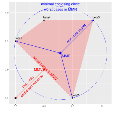
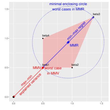
Figure 3.1: Illustration of MMV and MMR with four sub-population coefficients $\beta_{1},\beta_{2},\beta_{3},\beta_{4}\in\mathbb{R}^{2}$ and $\Sigma$ as the identity matrix. The MMV estimator is the closest point from $\mathcal{B}=\mathsf{conv}\{\beta_{1},\beta_{2},\beta_{3},\beta_{4}\}$ to the origin. The MMR estimator is the centroid of the minimal enclosing circle of $\mathcal{B}$. The squared distance between $\mathcal{B}$ and the origin is the max-min explained variance. The squared radius of the enclosing circle is the min-max regret. In the left plot, the supporting coefficients for MMV are $\beta_{1}$ and $\beta_{2}$, and the line segment joining them is the exposed face of worst cases for MMV. The supporting coefficients for MMR are $\beta_{1},\beta_{2},\beta_{3}$ on the enclosing circle, and the enclosing circle consists of the worst cases for MMR. In the right plot, $\beta_{1}$ is the only supporting coefficient for MMV, and $\beta_{1}$ itself is the MMV estimator. This corresponds to the “one-worst-case-dominate” phenomenon. In contrast, the supporting coefficients for MMR are $\beta_{1}$ and $\beta_{2}$, and the MMR estimator is not determined by a single sub-population coefficient.

In the following Theorem 2, we extend the characterization results for MMV in [23] and [11]. In particular, we further characterize the adversarial sub-populations that attain the max-min explained variance. The worst-case coefficients constitute an exposed face of $\mathcal{B}$, which is defined below.

Definition 2 ([30, Exposed Face, Section 18]).

Suppose $C\subseteq\mathbb{R}^{p}$ is convex and contained in a half-space, where the boundary hyperplane of the half-space is $H$. Then $F=C\cap H$ is called an exposed face of $C$.

Theorem 2 (Geometry of MMV).

Consider $\theta^{\star}$ as the solution to the MMV problem (7). Assume that $\Theta\supseteq\mathcal{B}$ and $\Sigma_{1}=\cdots=\Sigma_{K}=\Sigma>0$. We have

$$\theta^{\star}\in\mathop{\mathrm{argmin}}_{\theta\in\mathcal{B}}\|\theta\|_{\Sigma}^{2}.$$

Let $\mathcal{K}^{\star}=\left\{k:\langle\beta_{k},\theta^{\star}\rangle_{\Sigma}=\|\theta^{\star}\|_{\Sigma}^{2}\right\}$ be the supporting set. Then $\mathcal{B}^{\star}=\mathsf{conv}\{\beta_{k}\}_{k\in\mathcal{K}^{\star}}$ is an exposed face of $\mathcal{B}$, which consists of the worst cases that attain the max-min explained variance. That is, $V^{\star}=\max_{\theta\in\Theta}\min_{1\leq k\leq K}V_{\theta}(\beta_{k})=\|\theta^{\star}\|_{\Sigma}^{2}=V_{\theta^{\star}}(\beta)$ for any $\beta\in\mathcal{B}^{\star}$. Moreover, we have $\theta^{\star}\in\mathcal{B}^{\star}$, and $\theta^{\star}$ is also the worst-case coefficient that attains the max-min explained variance $V_{\theta^{\star}}(\theta^{\star})=V^{\star}$.

In terms of geometry, the MMV estimator is a convex combination of the worst-case sub-population coefficients. Such a convex combination is closest to the origin in terms of the ellipsoidal-norm based on $\Sigma$. The MMV estimator is also one of the worst-case coefficients attaining the max-min explained variance. As a consequence, the MMV estimator could be conservative when some sub-populations are exceptionally “poor” for linear regression. As an extreme case, if one of the sub-populations has a zero least-squares coefficient vector, or equivalently, the covariates are uncorrelated with the response variable on such a sub-population, then the best linear prediction on this sub-population has zero explained variance. Such a sub-population must be the worst case in Theorem 2, resulting in a zero MMV estimator. More generally, if on some mixture of the sub-populations, the covariates are uncorrelated with the response variable, then the MMV estimator becomes zero. Such a phenomenon suggests that MMV may be conservative when linear regression fits poorly on some adversarial sub-populations or their mixtures.

Theorem 2 suggests that the worst cases of MMV constitute an exposed face of $\mathcal{B}$, and the MMV estimator lies on such an exposed face. In comparison, we show in the following Theorem 3 that the worst cases of MMR constitute a bounding ellipsoid enclosing $\mathcal{B}$, and the MMR estimator is the centroid of such an ellipsoid.

Theorem 3 (Geometry of MMR).

Consider $\theta^{\star}$ as the solution to the $K$-MMR problem in Lemma 1. Assume that $\Theta\supseteq\mathcal{B}$ and $\Sigma_{1}=\cdots=\Sigma_{K}=\Sigma>0$. We have

$$(\theta^{\star},R^{\star})\in\mathop{\mathrm{argmin}}_{\theta\in\Theta,R\geq 0}\big{\{}R~{}\text{subject to}~{}\|\theta-\beta_{k}\|_{\Sigma}^{2}\leq R,~{}1\leq k\leq K\big{\}}.$$

In particular, $\mathcal{E}^{\star}=\{\beta\in\mathbb{R}^{p}:\|\theta^{\star}-\beta\|_{\Sigma}^{2}\leq R^{\star}\}$ is the minimal bounding ellipsoid enclosing $\mathcal{B}$. Let $\partial\mathcal{E}^{\star}=\{\beta\in\mathbb{R}^{p}:\|\theta^{\star}-\beta\|_{\Sigma}^{2}=R^{\star}\}$ be the boundary of $\mathcal{E}^{\star}$, and $\mathcal{K}^{\star}=\{k:\beta_{k}\in\partial\mathcal{E}^{\star}\}$ be the supporting set. Then $\partial\mathcal{E}^{\star}$ consists of the worst cases that attain the min-max regret. That is, $R^{\star}=\min_{\theta\in\Theta}\max_{1\leq k\leq K}R_{\theta}(\beta_{k})=R_{\theta^{\star}}(\beta)$ for any $\beta\in\partial\mathcal{E}^{\star}$. Moreover, we have $\theta^{\star}\in\mathsf{conv}\{\beta_{k}\}_{k\in\mathcal{K}^{\star}}$, and $R_{\theta^{\star}}(\theta^{\star})=0$.

Similar to MMV, the MMR estimator can also be represented as a convex combination of the worst-case coefficients. In terms of geometry, it corresponds to the centroid of the bounding ellipsoid $\mathcal{E}^{\star}$ such that $\mathcal{E}^{\star}\supseteq\mathcal{B}$. The boundary of such an ellipsoid $\partial\mathcal{E}^{\star}$ consists of the worst cases of MMR, which is determined by the supporting coefficients $\{\beta_{k^{\star}}\}_{k^{\star}\in\mathcal{K}^{\star}}$ on this boundary. In contrast to MMV, the MMR estimator is not a worst-case sub-population coefficient. Instead, it corresponds to the most favorable sub-population on which the MMR estimator incurs no regret.

We further establish the connection between MMV and MMR through their dual optimization problems in the following Proposition 4. In particular, both estimators are convex aggregations of sub-population coefficients, and their dual problems optimize for different objectives over the convex aggregation weights. The supports of the optimized weights are also the supporting sets for their respective worst cases.

Proposition 4 (Duality for MMV and MMR).

Consider the same setups and assumptions as in Theorems 2 and 3, where $\theta_{\mathrm{MMV}}^{\star}$ and $\theta_{\mathrm{MMR}}^{\star}$ are the MMV and MMR estimators, corresponding to the max-min explained variance $V^{\star}$, min-max regret $R^{\star}$, and the supporting sets of worst cases $\mathcal{K}_{\mathrm{MMV}}^{\star}$ for MMV, and $\mathcal{K}_{\mathrm{MMR}}^{\star}$ for MMR, respectively. Let $\mathsf{B}=[\beta_{1};\cdots;\beta_{K}]\in\mathbb{R}^{p\times K}$ be the matrix of sub-population coefficients, $\mathsf{G}=\mathsf{B}^{\intercal}\Sigma\mathsf{B}\in\mathbb{R}^{K\times K}$ be the associated Gram matrix, and $\mathsf{d}=(\mathsf{G}_{11},\cdots,\mathsf{G}_{KK})^{\intercal}$ be the diagonal vector of $\mathsf{G}$. Then we have $\theta_{\mathrm{MMV}}^{\star}=\mathsf{B}\gamma_{\mathrm{MMV}}^{\star}$ and $\theta_{\mathrm{MMR}}^{\star}=\mathsf{B}\gamma_{\mathrm{MMR}}^{\star}$, where

$$\gamma_{\mathrm{MMV}}^{\star}\in\mathop{\mathrm{argmin}}_{\gamma\in\Delta^{K-1}}\big{\{}\mathcal{V}(\gamma)=\gamma^{\intercal}\mathsf{G}\gamma\big{\}};\quad\gamma_{\mathrm{MMR}}^{\star}\in\mathop{\mathrm{argmax}}_{\gamma\in\Delta^{K-1}}\big{\{}\mathcal{R}(\gamma)=\mathsf{d}^{\intercal}\gamma-\gamma^{\intercal}\mathsf{G}\gamma\big{\}}.$$

Moreover, $V^{\star}=\mathcal{V}(\gamma_{\mathrm{MMV}}^{\star})$, $R^{\star}=\mathcal{R}(\gamma_{\mathrm{MMR}}^{\star})$, $\mathcal{K}_{\mathrm{MMV}}^{\star}=\big{\{}k:\gamma_{\mathrm{MMV},k}^{\star}>0\big{\}}$, and $\mathcal{K}_{\mathrm{MMR}}^{\star}=\big{\{}k:\gamma_{\mathrm{MMR},k}^{\star}>0\big{\}}$. There exists a dual optimal solution to MMV such that $|\mathcal{K}_{\mathrm{MMV}}^{\star}|=1$ if and only if $\mathcal{K}_{\mathrm{MMV}}^{\star}=\{k^{\star}\}$ and $\|\beta_{k^{\star}}\|_{\Sigma}^{2}\leq\min_{k\neq k^{\star}}\langle\beta_{k^{\star}},\beta_{k}\rangle_{\Sigma}$. In contrast, there exists a dual optimal solution to MMR such that $|\mathcal{K}_{\mathrm{MMR}}^{\star}|=1$ if and only if $\beta_{1}=\cdots=\beta_{K}$.

Remark 1 (Convex Aggregations).

In Proposition 4, both the MMV and MMR estimators are characterized in the form $\theta^{\star}=\mathsf{B}\gamma^{\star}=\sum_{k=1}^{K}\gamma_{k}^{\star}\beta_{k}$, which can be viewed as the least-squares coefficient on the mixture of sub-populations $\sum_{k=1}^{K}\gamma_{k}^{\star}\mathbb{P}^{(\xi_{k})}$.

The dual objectives for MMV and MMR differ in the term $\mathsf{d}^{\intercal}\gamma$, which leads to different aggregation weights in their estimators. To shed more lights on their relationships, suppose the linear system $2\mathsf{G}\gamma^{\circ}-\mathsf{d}=0$ has a feasible solution $\gamma^{\circ}\in\mathbb{R}^{K}$. Note that $\gamma^{\circ}\notin\Delta^{K-1}$ in general. The dual problem for MMR in Proposition 4 can be further written as $\gamma_{\mathrm{MMR}}^{\star}\in\mathop{\mathrm{argmin}}_{\gamma\in\Delta^{K-1}}\left(\gamma-\gamma^{\circ}\right)^{\intercal}\mathsf{G}\left(\gamma-\gamma^{\circ}\right)$. It is then clear that MMV attracts the aggregation weight vector $\gamma_{\mathrm{MMV}}^{\star}$ to zero, while MMR attracts $\gamma_{\mathrm{MMR}}^{\star}$ to $\gamma^{\circ}$. For the MMR problem, we further establish in the following Lemma 2 that, $\gamma_{\mathrm{MMR}}^{\star}$ can be viewed as the projection of any equi-regret weight vector onto $\Delta^{K-1}$. In this way, MMR aims to achieve regret parity [9] among sub-populations.

Lemma 2.

Consider the dual problem for MMR in Proposition 4. Define the class of equi-regret linear aggregation weights $\Gamma=\big{\{}\gamma=(\gamma_{1},\cdots,\gamma_{K})^{\intercal}\in\mathbb{R}^{K}:R_{\theta}(\beta_{1})=\cdots=R_{\theta}(\beta_{K}),~{}\theta=\sum_{k=1}^{K}\gamma_{k}\beta_{k}\big{\}}$. If $2\mathsf{G}\gamma^{\circ}-\mathsf{d}=0$ has a feasible solution $\gamma^{\circ}\in\mathbb{R}^{K}$, then $\Gamma\neq\emptyset$ and $\gamma^{\circ}\in\Gamma$. For any $\widetilde{\gamma}^{\circ}\in\Gamma$, we have $\gamma_{\mathrm{MMR}}^{\star}\in\mathop{\mathrm{argmin}}_{\gamma\in\Delta^{K-1}}\big{(}\gamma-\widetilde{\gamma}^{\circ}\big{)}^{\intercal}\mathsf{G}\big{(}\gamma-\widetilde{\gamma}^{\circ}\big{)}$.

In terms of the supporting sets $\mathcal{K}_{\mathrm{MMV}}^{\star}$ and $\mathcal{K}_{\mathrm{MMR}}^{\star}$, our Proposition 4 further characterizes the “one-worst-case-dominate” phenomenon through the conditions for $|\mathcal{K}_{\mathrm{MMV}}^{\star}|=1$ and $|\mathcal{K}_{\mathrm{MMR}}^{\star}|=1$. For MMV, the worst case $k^{\star}$ could dominate when its sub-population least-squares explained variance $\|\beta_{k^{\star}}\|_{\Sigma}^{2}=\mathsf{Cov}^{(\xi_{k^{\star}})}(\bm{X}^{\intercal}\beta_{k^{\star}},Y)$ is smaller than the explained variance $\langle\beta_{k^{\star}},\beta_{k}\rangle_{\Sigma}=\mathsf{Cov}^{(\xi_{k})}(\bm{X}^{\intercal}\beta_{k^{\star}},Y)$ when $\beta_{k^{\star}}$ is deployed to the $k$-th sub-population for $k\neq k^{\star}$. One example could be referred to the right plot in Figure 3.1. Such an adversarial case could happen if linear regression is fitted poorly on the $k^{\star}$-th sub-population. In contrast, as long as the sub-populations have certain heterogeneity, such that their least-squares coefficients are not identical, MMR would never be dominated by a single sub-population.

Before the end of this section, we also note that the MMR estimator can certify certain guarantee in terms of the worst-case explained variance criterion. Specifically, the following Proposition 5 suggests that the sub-optimality of the MMR estimator in terms of the worst-case explained variance is at most the amount of min-max regret $R^{\star}$. If $R^{\star}$ is relatively small compared to the amount of max-min explained variance $V^{\star}$, then the MMR estimator can also be approximately optimal in the worst-case explained variance criterion.

Proposition 5.

Consider the same setups and assumptions as in Theorems 2 and 3. With the max-min explained variance $V^{\star}$ and the min-max regret $R^{\star}$, the MMR estimator $\theta_{\rm MMR}^{\star}$ satisfies $V^{\star}-\min_{1\leq k\leq K}V_{\theta_{\rm MMR}^{\star}}(\beta_{k})\leq R^{\star}$.

4 Theoretical Properties

In this section, we consider the theoretical properties of $\widehat{\theta}_{K,n}$ as the solution to the general empirical MMR problem (4). Here, the indices $K$ and $n$ indicate the observed $K$ groups and the total sample size $n$, respectively. We aim to establish the excess worst-case regret guarantees for the empirical MMR relative to the $K$-min-max regret $\min_{\theta\in\Theta}\max_{1\leq k\leq K}R_{\theta}(\xi_{k})$ in Section 4.1, and the $\mathbb{P}$-min-max regret $\inf_{\theta\in\Theta}\sup_{\zeta\in\Xi}R_{\theta}(\zeta)$ in Section 4.2, respectively.

4.1 Guarantees in the $K$-MMR Criterion

We consider two sets of generic conditions that can be established based on the concentration theories for ERM. In particular, within each group, as the per-group sample size is sufficiently large, these conditions require that the within-group empirical risk difference concentrates at the sub-population risk difference with high probability. For $1\leq k\leq K$, we denote $\beta_{k}\in\mathop{\mathrm{argmin}}_{\beta\in\Theta}\mathbb{E}^{(\xi_{k})}\big{[}\ell_{\beta}\big{(}Z_{1}^{(k)}\big{)}\big{]}$ as the sub-population risk minimizer.

Condition 1a.

For every $1\leq k\leq K$ and $t\geq 0$, with $\mathbb{P}^{(\xi_{k})}$-probability at least $1-2e^{-t}$, we have

$$\sup_{\theta\in\Theta}\left|{1\over n_{k}}\sum_{i=1}^{n_{k}}\left[\ell_{\theta}\big{(}Z_{i}^{(k)}\big{)}-\ell_{\beta_{k}}\big{(}Z_{i}^{(k)}\big{)}\right]-\mathbb{E}^{(\xi_{k})}\left[\ell_{\theta}\big{(}Z_{1}^{(k)}\big{)}-\ell_{\beta_{k}}\big{(}Z_{1}^{(k)}\big{)}\right]\right|\leq r_{n_{k}}(t),$$

for some $r_{n_{k}}(t)$ as a deterministic upper bound that depends on the sample size $n_{k}$ for the $k$-th group and the parameter $t\geq 0$.

Condition 1b ([2]).

For every $1\leq k\leq K$, $t\geq 0$ and $\eta>1$, with $\mathbb{P}^{(\xi_{k})}$-probability at least $1-2e^{-t}$, for all $\theta\in\Theta$, we have

$$\mathbb{E}^{(\xi_{k})}\left[\ell_{\theta}\big{(}Z_{1}^{(k)}\big{)}-\ell_{\beta_{k}}\big{(}Z_{1}^{(k)}\big{)}\right]\leq{\eta\over\eta-1}{1\over n_{k}}\sum_{i=1}^{n_{k}}\left[\ell_{\theta}\big{(}Z_{i}^{(k)}\big{)}-\ell_{\beta_{k}}\big{(}Z_{i}^{(k)}\big{)}\right]+\eta r_{n_{k}}^{2}(t);$$

$${1\over n_{k}}\sum_{i=1}^{n_{k}}\left[\ell_{\theta}\big{(}Z_{i}^{(k)}\big{)}-\ell_{\beta_{k}}\big{(}Z_{i}^{(k)}\big{)}\right]\leq{\eta+1\over\eta}\mathbb{E}^{(\xi_{k})}\left[\ell_{\theta}\big{(}Z_{1}^{(k)}\big{)}-\ell_{\beta_{k}}\big{(}Z_{1}^{(k)}\big{)}\right]+\eta r_{n_{k}}^{2}(t),$$

for some $r_{n_{k}}(t)$ as a deterministic upper bound that depends on the sample size $n_{k}$ for the $k$-th group and the parameter $t\geq 0$.

Note that Condition 1a is a general uniform concentration condition, but could lead to a sub-optimal rate in $r_{n_{k}}(t)$. If $\Theta$ has a finite VC dimension $\mathfrak{C}<+\infty$, then $r_{n_{k}}(t)$ is typically $\mathcal{O}(\sqrt{(\mathfrak{C}+t)/n_{k}})$. Condition 1b is motivated from the local Rademacher complexities [22, 2]. In particular, if the loss is uniformly bounded, and the following variance-expectation condition holds: $\mathsf{Var}^{(\xi_{k})}\big{[}\ell_{\theta}\big{(}Z_{1}^{(k)}\big{)}-\ell_{\beta_{k}}\big{(}Z_{1}^{(k)}\big{)}\big{]}\leq B\mathbb{E}^{(\xi_{k})}\big{[}\ell_{\theta}\big{(}Z_{1}^{(k)}\big{)}-\ell_{\beta_{k}}\big{(}Z_{1}^{(k)}\big{)}\big{]}$ for some universal constant $B<+\infty$, then Condition 1b could be established with a “fast rate” $r_{n_{k}}^{2}(t)$ compared to the standard rate $r_{n_{k}}(t)$ in Condition 1a. Such a variance-expectation condition can be satisfied if the loss $\theta\mapsto\ell_{\theta}\big{(}Z_{1}^{(k)}\big{)}$ is uniformly Lipschitz and strongly convex.

Based on either of Conditions 1a and 1b, we establish the following excess $K$-MMR guarantee for the empirical MMR. In particular, we take the “union bound” of $K$ per-group concentrations, which contributes to a $\log K$ term in the resulting excess $K$-MMR bound.

Theorem 6 (Excess $K$-MMR Guarantee).

Suppose $\widehat{\theta}_{K,n}$ solves the empirical MMR problem (4), and $\mathcal{R}_{K}^{\star}=\min_{\theta\in\Theta}\max_{1\leq k\leq K}R_{\theta}(\xi_{k})$ is the $K$-min-max regret. Assume either of Conditions 1a and 1b. Let $r(t)=\max_{1\leq k\leq K}r_{n_{k}}(t+\log K)$. Then for every $t\geq 0$, with probability at least $1-2e^{-t}$ conditional on $\xi_{1},\cdots,\xi_{K}$, we have

$$\max_{1\leq k\leq K}R_{\widehat{\theta}_{K,n}}(\xi_{k})-\mathcal{R}_{K}^{\star}\leq\begin{cases}4r(t),&\text{under Condition \ref{cond:regret_error}};\\ 4\sqrt{3\mathcal{R}_{K}^{\star}}r(t)+(4+2\sqrt{6})r^{2}(t),&\text{under Condition \ref{cond:regret_error_local}}.\end{cases}$$

Remark 2 (Fast Rate with Homogeneous Sub-Populations).

Under Condition 1b, a fast rate $r^{2}(t)$ can be possible if $\mathcal{R}_{K}^{\star}=0$, that is, $\beta_{1}=\cdots=\beta_{K}$. For example, [2, Corollary 3.7] established Condition 1b with $r_{n}^{2}(t)=\mathcal{O}\big{(}{\mathfrak{C}\log(n/\mathfrak{C})+t\over n}\big{)}$, where $\mathfrak{C}$ is the VC-dimension of $\Theta$. Then Theorem 6 implies the same rate if the sub-populations are homogeneous. A similar phenomenon was pointed out by [2, Section 5.2] and [1, Theorem 4].

4.2 Guarantees in the $\mathbb{P}$-MMR Criterion

In this section, we further establish the generalizability of robustness beyond the $K$ realized sub-populations in terms of the $\mathbb{P}$-MMR criterion. Specifically, we consider $\{\xi_{k}\}_{k=1}^{K}$ as IID observed instances of the random element $\xi$ from the super-population. That is, the observed sub-populations $\mathbb{P}^{(\xi_{1})},\cdots,\mathbb{P}^{(\xi_{K})}$ are realizations of the random sub-population $\mathbb{P}^{(\xi)}$. As a result, for every $\theta\in\Theta$, the regret $R_{\theta}(\xi)$ is a real-valued random variable, where the randomness is due to $\xi$. We call such a random variable as the regret profile. For fixed $\theta\in\Theta$, the randomness of the regret profile $R_{\theta}(\xi)$ is due to the sampling of a sub-population $\mathbb{P}^{(\xi)}$ and the regret heterogeneity among realizable sub-populations $\{R_{\theta}(\zeta)\}_{\zeta\in\Xi}$.

Suppose for every fixed $\theta\in\Theta$, the worst-case regret $\mathcal{R}(\theta)=\sup_{\zeta\in\Xi}R_{\theta}(\zeta)$ among the super-population is finite. Then $\mathbb{P}$-MMR aims to solve the super-population MMR problem $\min_{\theta\in\Theta}\mathcal{R}(\theta)$. In practice, we only observe $K$ realizations $\xi_{1},\cdots,\xi_{K}$ of $\xi$ and compute $\widehat{\mathcal{R}}_{K}(\theta)=\max_{1\leq k\leq K}R_{\theta}(\xi_{k})$. Then we anticipate that under certain conditions, as the number of groups $K$ increases, we have $\widehat{\mathcal{R}}_{K}(\theta)\to\mathcal{R}(\theta)$ for every fixed $\theta$, and uniformly over $\theta\in\Theta$. Such a goal motivates the following concentration condition for the regret profile.

Condition 2 (Locally Sub-Weibull Regret Profile).

There exists some universal parameters $\alpha,t_{0}>0$ and $\nu<+\infty$, such that for every $\theta\in\Theta$, the support of $R_{\theta}(\xi)$ has a finite upper limit $\mathcal{R}(\theta)<+\infty$, and $\mathcal{R}(\theta)-R_{\theta}(\xi)$ is locally sub-Weibull with the order parameter $\alpha$ and the scale parameter $\nu$ in a $t_{0}$-neighborhood of 0. That is,

$$\mathbb{P}\left\{\mathcal{R}(\theta)-R_{\theta}(\xi)\leq\nu t\right\}\geq 1-e^{-t^{\alpha}};\quad 0\leq t\leq t_{0}.$$

Condition 2 is motivated from the sufficient and necessary condition for the weak convergence of $K^{1/\alpha}\big{\{}\mathcal{R}(\theta)-\widehat{\mathcal{R}}_{K}(\theta)\big{\}}$ to a Weibull-type extreme value distribution [6] for fixed $\theta\in\Theta$. We further require that the parameters $\alpha,\nu,t_{0}$ are universal constants across all $\theta\in\Theta$, which is necessary for such a weak convergence to be simultaneous.

Let $\mathscr{R}=\{R_{\theta}(\xi):\theta\in\Theta\}$ be the class of regret profiles, which is considered as a class of measurable functions of the random element $\xi$. We assume a parametric complexity for $\mathscr{R}$ in terms of the bracketing number.

Condition 3 (Complexity for the Class of Regret Profiles).

There exists a universal constant $0<A<+\infty$ and a finite $\mathfrak{C}<+\infty$, such that $\log\mathcal{N}_{[]}(r,\mathscr{R},\mathcal{L}^{\infty})\leq\mathfrak{C}\log{A\over r}$ for $0\leq r\leq A$. Here, $\mathcal{N}_{[]}(r,\mathscr{R},\mathcal{L}^{\infty}(\mathbb{P}))$ is the minimum number of $r$-brackets in $\mathcal{L}^{\infty}$ to cover $\mathscr{R}$.

With Conditions 2 and 3 in addition to either of Conditions 1a and 1b, we are able to establish the following $\mathbb{P}$-MMR guarantee for the empirical MMR.

Theorem 7 (Excess $\mathbb{P}$-MMR Guarantee).

Suppose $\widehat{\theta}_{K,n}$ solves the empirical MMR problem (4), and $\mathcal{R}^{\star}=\inf_{\theta\in\Theta}\mathcal{R}(\theta)$ is the $\mathbb{P}$-min-max regret. Assume Conditions 2, 3 and either of Conditions 1a and 1b. Let $r_{K}(t)=\max_{1\leq k\leq K}r_{n_{k}}(t+\log K)$ and $r_{\mathbb{P}}(t)=(\max\{1,\alpha^{-1/\alpha}\}+A)\nu\left({\mathfrak{C}\log(K/\mathfrak{C})+\mathfrak{C}\log(1/\nu)+t\over K}\right)^{1/\alpha}$. Then for every $K,t\geq 0$ satisfying ${\mathfrak{C}\over K}\big{(}{1\over\alpha}\log{K\over\mathfrak{C}}+\log{1\over\nu}\big{)}\leq t_{0}^{\alpha}/2$ and $t\leq t_{0}^{\alpha}K/2$, with probability at least $1-3e^{-t}$, we have

$$\mathcal{R}(\widehat{\theta}_{K,n})-\mathcal{R}^{\star}\leq\begin{cases}4r_{K}(t)+r_{\mathbb{P}}(t),&\text{under Condition \ref{cond:regret_error}};\\ 4\sqrt{3\mathcal{R}^{\star}}r_{K}(t)+(4+2\sqrt{6})r_{K}^{2}(t)+r_{\mathbb{P}}(t),&\text{under Condition \ref{cond:regret_error_local}}.\end{cases}$$

Compared to Theorem 6, the results in Theorem 7 incorporate the additional generalization error $r_{\mathbb{P}}(t)$ due to the concentration of $\big{\{}\mathcal{R}(\theta)-\widehat{\mathcal{R}}_{K}(\theta)\big{\}}_{\theta\in\Theta}$. If the rate of convergence in Condition 1a or 1b is $r_{n_{k}}(t)=\mathcal{O}(\sqrt{(\mathfrak{C}+t)/n_{k}})$, then the excess $\mathbb{P}$-MMR bound is $\mathcal{O}_{\mathbb{P}}\Big{(}\sqrt{\mathfrak{C}+\log K\over n_{\min}}+\big{(}{\mathfrak{C}\log(K/\mathfrak{C})\over K}\big{)}^{1/\alpha}\Big{)}$ with $n_{\min}=\min_{1\leq k\leq K}n_{k}$. Moreover, analogous to Remark 2, a fast rate $\mathcal{O}_{\mathbb{P}}\big{(}{\mathfrak{C}+\log K\over n_{\min}}+\big{(}{\mathfrak{C}\log(K/\mathfrak{C})\over K}\big{)}^{1/\alpha}\big{)}$ could be achieved if $\mathcal{R}^{\star}=0$, in which case all realizable sub-populations are homogeneous.

We further instantiate the excess $\mathbb{P}$-MMR guarantee for the linear regression setting in Section 3. To satisfy Conditions 1a, 2, 3, the following two assumptions are sufficient. More details on justifying these conditions are discussed in Supplemental Material E.5.

Assumption 3 (Sub-Gaussianity).

On every sub-population $\mathbb{P}^{(\xi_{k})}$, both $\Sigma_{k}^{-1/2}\bm{X}$ and $\Sigma_{k}^{-1/2}\bm{X}(Y-\bm{X}^{\intercal}\beta_{k})$ are sub-Gaussian with the universal parameter $\widebar{\sigma}^{2}<+\infty$ in Assumption 2.

Assumption 4 (Sub-Weibull).

Denote $\beta(\xi)=\mathop{\mathrm{argmin}}_{\beta\in\Theta}\mathbb{E}^{(\xi)}(Y-\bm{X}^{\intercal}\beta)^{2}$ and $\Sigma(\xi)=\mathbb{E}^{(\xi)}(\bm{X}\bm{X}^{\intercal})$. Assume that there exist some universal parameters $\alpha,t_{0}>0$ and $\nu_{\beta},\nu_{\Sigma}<+\infty$, such that for every fixed $\zeta\in\Xi$, we have

$$\mathbb{P}\left\{\big{\|}\beta(\xi)-\beta(\zeta)\big{\|}_{2}\leq\nu_{\beta}t,\big{\|}\Sigma(\xi)-\Sigma(\zeta)\big{\|}_{2}\leq\nu_{\Sigma}t\right\}\geq 1-e^{-t^{\alpha}};\quad 0\leq t\leq t_{0}.$$

Corollary 8 (Excess $\mathbb{P}$-MMR Guarantee for Linear Regression).

Consider the setup in Theorem 7 for the linear regression problem under Assumptions 1, 2, 3, 4. Let $D=\sup_{\theta_{1},\theta_{2}\in\Theta}\|\theta_{1}-\theta_{2}\|_{2}$, $\nu=2D\widebar{\lambda}\nu_{\beta}+D^{2}\nu_{\Sigma}$. Then there exists some universal constant $C<+\infty$, such that for every $n_{\min},K,t\geq 0$ satisfying $n_{\min}\geq p$, ${p\over K}\big{(}{1\over\alpha}\log{K\over p}+\log{1\over\nu}\big{)}\leq t_{0}^{\alpha}/2$ and $t\leq\min\{n_{\min},t_{0}^{\alpha}K/2\}$, with probability at least $1-3e^{-t}$, we have

$$\mathcal{R}(\widehat{\theta}_{K,n})-\mathcal{R}^{\star}\leq \quad C(2D\widebar{\lambda}^{1/2}\widebar{\sigma}+D^{2}\widebar{\lambda}\widebar{\sigma}^{2})\sqrt{p+\log K+t\over n_{\min}}$$

$$+(\max\{1,\alpha^{-1/\alpha}\}+1.5D)\nu\left({p\log(K/p)+p\log(1/\nu)+t\over K}\right)^{1/\alpha}.$$

5 Simulation Studies

In this section, we compare the proposed MMR approach with the pooled ERM, GDRO, and MMV in terms of the robustness and generalizability on extensive numerical studies. To assess the robustness against various sources of heterogeneity, we generate data from multiple linear models. In this setup, we sample regression coefficients for each linear model from a mixture of two uniform distributions. By altering the weights between two uniforms, it is flexible to examine the impact of the distribution of regression coefficients on four methods. Specifically, we first sample $c=1$ with probability $\pi$ and $c=0$ with probability $1-\pi$. Then we randomly generate the regression coefficients from $\mathsf{Uniform}(\mathsf{B}_{c})$, where $\mathsf{B}_{0}$ is the unit ball centered at $(1,3\times\bm{1}_{p-1}^{\top})^{\top}$ and $\mathsf{B}_{1}$ is the ball centered at $3\times\bm{1}_{p}$ with radius $3$. Let $\Theta=\mathsf{B}_{0}\cup\mathsf{B}_{1}$ be the parameter space. Following the above data generation process, we independently sample the regression coefficients $\{\beta_{k}\}_{k=1}^{K}$ for $K=100$ groups. For each group given $\beta_{k}$, we further generate the data $\{\bm{X}_{i}^{(k)},Y_{i}^{(k)}\}_{i=1}^{n_{k}}$ based on the following linear regression model: $\bm{X}_{i}^{(k)}\sim\mathcal{N}(\mathbf{0},\mathsf{I}_{p})$, $\epsilon_{i}^{(k)}\sim\mathcal{N}(0,p+\sigma^{2}\|\beta_{k}\|_{2}^{2})$, $\bm{X}_{i}^{(k)}\mathchoice{\mathrel{\hbox to0.0pt{$\displaystyle\perp$\hss}\mkern 2.0mu{\displaystyle\perp}}}{\mathrel{\hbox to0.0pt{$\textstyle\perp$\hss}\mkern 2.0mu{\textstyle\perp}}}{\mathrel{\hbox to0.0pt{$\scriptstyle\perp$\hss}\mkern 2.0mu{\scriptstyle\perp}}}{\mathrel{\hbox to0.0pt{$\scriptscriptstyle\perp$\hss}\mkern 2.0mu{\scriptscriptstyle\perp}}}\epsilon_{i}^{(k)}$, and $Y_{i}^{(k)}={\bm{X}_{i}^{(k)\intercal}}\beta_{k}+\epsilon_{i}^{(k)}.$ Here, the within-group Bayes risk $p+\sigma^{2}\|\beta_{k}\|_{2}^{2}$ depends on the group coefficient $\beta_{k}$. The larger $\sigma^{2}$ leads to a larger magnitude of the cross-group heteroscedasticity. We set $\pi=0.2$, $\sigma^{2}=0.5$, and the sample size per group as $n_{k}=1,000$ by default.

We compare four methods in four different settings. The first three settings investigate three types of robustness properties, respectively, including group distributional shift, heteroscedasticity invariance, and regression equivariance. The fourth setting further considers the impact of varying the number of groups and the sample size per group.

Specifically, for the first three settings, we visualize the estimator of each method given infinite sample points from all realizable sub-populations. In particular, we examine the impact of different types of heterogeneity on their locations. Subsequently, for each of the four settings, we evaluate the generalizability of the prediction performance of their empirical estimates. We report the worst-case regret, risk, unexplained variance, and the average risk on $K_{\rm test}=10,000$ testing sub-populations, where the regression coefficients $\big{\{}\beta_{k}^{(\operatorname{test})}\big{\}}_{k=1}^{K_{\rm test}}$ are independently sampled from the aforementioned mixture of two uniforms. Such testing regression coefficients are generally different from the training ones, which helps to assess the generalizability of methods to those unseen sub-populations drawn from the same super-population. More details for the evaluation metrics are provided in Supplemental Material F.

5.1 Setting 1: Invariance to Group Distributional Shift

In this subsection, we investigate the invariance property of four methods to the group distributional shift. In particular, group distributional shift is common in real-world applications. For example, it often occurs when the observed data are not sufficiently representative of all possible sub-populations. To mimic this situation, we vary the weight $\pi$ between two uniform distributions when sampling regression coefficients for each group. As $\pi$ decreases, we observe more data from more groups whose regression coefficients are sampled from $\mathsf{B}_{0}$.

For ease of visualization, we first set $p=2$ and plot the sampled regression coefficients as circles in Figure 5.1. Darker colors and larger sizes of the circles indicate higher Bayes risks. Figure 5.1 shows the locations of four estimators when $\pi=1,0.5,0.2$ from left to right respectively. When $\pi=1$, the pooled estimator coincides with our MMR estimator. As $\pi$ decreases, there are more groups with regression coefficients sampled on the left side. As a result, the pooled estimator deviates towards the left. In contrast, the other population estimators remain the same. In particular, as suggested by geometric characterization in Section 3.2, the MMR estimator remains at the centroid of the minimal bounding ellipsoid of the support $\Theta$. The MMV estimator is the one in $\Theta$ that is closest to the origin.

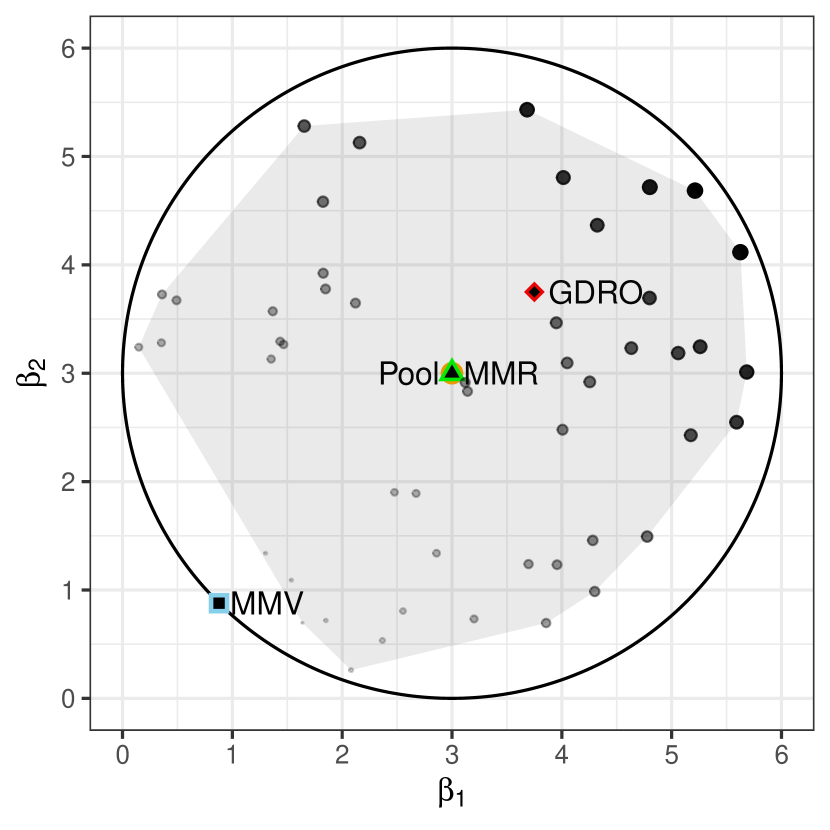
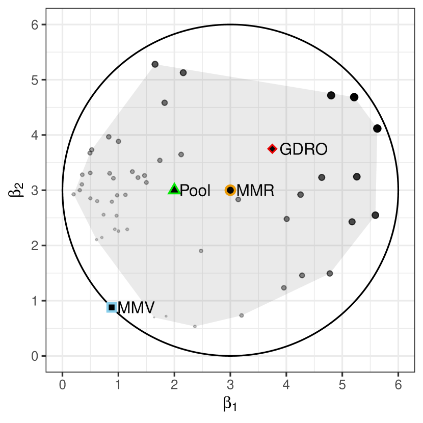
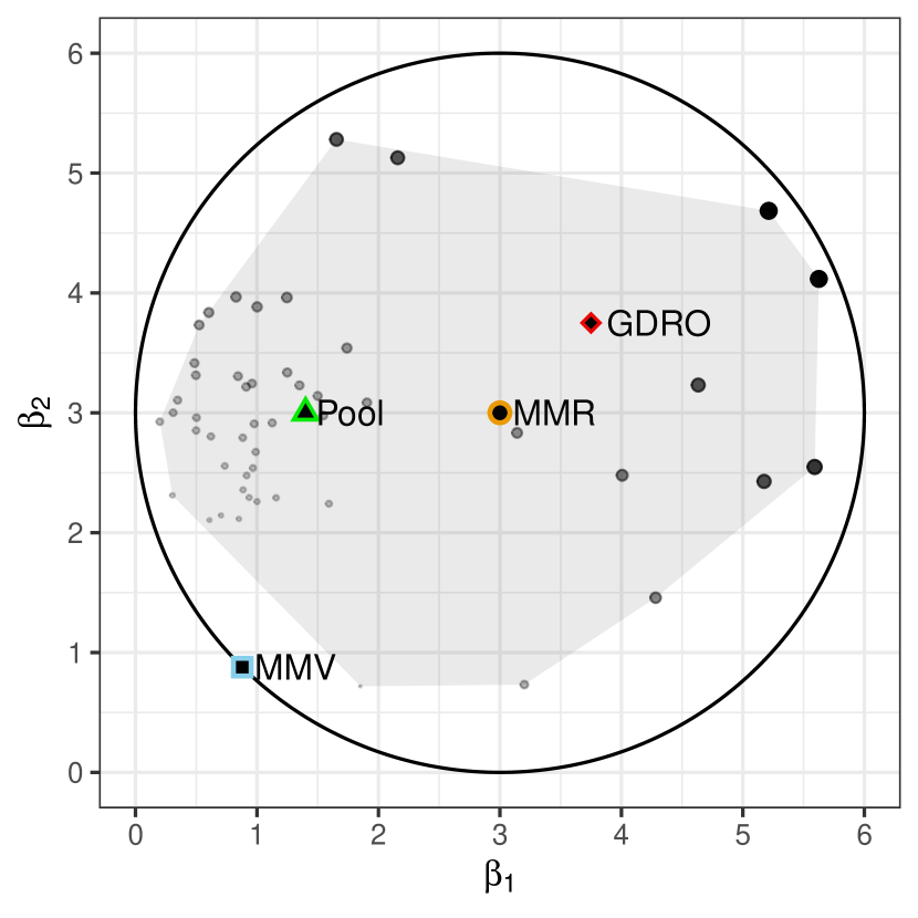
Figure 5.1: Locations of four population estimators in the presence of group distributional shift. Left: $\pi=1$; Middle: $\pi=0.5$; Right: $\pi=0.2$.

We further set $p=5$ and vary $\pi$ in the range of $\{0.2,0.4,0.6,0.8,1.0\}$ to assess the generalizability of the prediction performance of their empirical estimates. Figure F.3 in the Supplemental Material summarizes the results, where each row corresponds to a particular evaluation metric. As expected, each of the four methods performs almost the best in terms of the evaluation metrics that they aim to optimize for, respectively. The testing worst-case regrets for these methods are provided in Figure 5.2. As shown in the first column, the pooled estimate that optimizes the empirical average risk is more sensitive to the group distributional shift than the other three estimates. As $\pi$ decreases, the pooled estimate experiences a substantial increase in the worst-case regret. In contrast, the MMR, GDRO, and MMV estimates perform stably at various $\pi$ values. When $\pi=1$, i.e., the pooled estimator coincides with the MMR estimator, their empirical estimates achieve almost the same prediction performance.

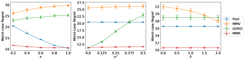
Figure 5.2: The worst-case regret for four empirical estimates on the test data. From left to right: the results under group distributional shift, heteroscedasticity, and additive homogeneous effect.

5.2 Setting 2: Invariance to Heteroscedasticity

We study the heteroscedasticity invariance property of four methods by varying the heterogeneity of the Bayes risks across groups. In particular, the Bayes risk of the $k$-th group is $p+\sigma^{2}\|\beta_{k}\|_{2}^{2}$, which is identical across $k$’s if $\sigma^{2}=0$. As $\sigma^{2}$ increases, the magnitude of group heteroscedasticity grows.

Figure F.1 in the Supplemental Material shows how the locations of four population estimators vary in the presence of heteroscedasticity. When $\sigma^{2}=0$ and there is no heteroscedasticity, the GDRO estimator aligns with the MMR estimator. However, as $\sigma^{2}$ gradually increases, the GDRO estimator shifts while the other estimators remain unchanged. In particular, the GDRO estimator moves closer to the groups with larger Bayes risks. When certain groups have substantially larger Bayes risks than the others, they dominate the worst-case risk optimization of GDRO. In the extreme case, this may lead to the degeneration of GDRO as discussed in Table 3.1.

In addition, we compare the prediction performance of their empirical estimates when varying $\sigma^{2}$ in the range of $\{0,0.125,0.25,0.375,0.5\}$. In the second column of Figure 5.2, the worst-case regret of the GDRO estimate increases substantially as $\sigma^{2}$ becomes large, while the other three estimates perform robustly. This suggests that in the presence of groups with high Bayes risks, the performance of GDRO is predominantly driven by these groups, and its performance on the other groups may be overlooked.

5.3 Setting 3: Regression Equivariance

We further investigate the regression equivariance property of four methods. Consider an additive homogeneous effect $\delta\times\bm{1}_{p}$ on the regression coefficients, that is, the coefficients for each group increase by the same amount $\delta$ entrywise. A methood with the regression equivariance property would preserve this additive homogeneous effect. Figure F.2 in the Supplemental Material shows the locations of four population estimators when $\delta=0,-1,-2$ from left to right, respectively. We can see that all estimators except for the MMV estimator are shifted by the same amount, and thereby suggest their regression equivariance property. In comparison, the MMV estimator is drawn towards zero and may even degenerate to exactly zero when the support set covers the origin.

We apply the same homogeneous effect to the test data and evaluate the prediction performance of the empirical estimates. We vary $\delta$ in the range of $\{0,0.5,1,1.5,2\}$. The third column of Figure 5.2 indicates that the MMV estimate suffers from instability in the worst-case regret due to the lack of equivariance property.

Overall, as discussed in Section 3, the MMR estimator enjoys the invariance and equivariance properties simultaneously. It also achieves robust prediction performance under various heterogeneities, and enjoys the lowest worst-case regret when compared to the other three estimates.

5.4 Setting 4: Varying Sample Size per Group and Group Size

Finally, we examine the effect of varying the training sample size per group and the number of groups. We first set the number of groups as $25$ and vary the sample size per group from $100$ to $1,600$. The results are provided in Figure F.4 in the Supplemental Material. As shown on the left of Figure F.4, the stable curve observed for large sample sizes suggests the convergence of the worst-case regret of the empirical estimate. Moreover, we set the sample size as $1,000$ and vary the number of groups from $25$ to $400$. As shown on the right of Figure F.4, the MMR method further improves its generalizability after observing data from more sub-populations. These confirm the theoretical guarantees in Section 4.

6 Kidney Transplantation Data Example

In this section, we apply the proposed method to mortality risk prediction after kidney transplantation and investigate its robustness against various data perturbations. Kidney transplantation is the primary renal replacement therapy for patients suffering from end-stage renal disease, a lethal and costly disease with increasing incidence rates and healthcare expenditures [33]. Successful kidney transplantation can significantly improve patient outcomes and reduce healthcare expenses compared to dialysis. However, the demand for donor kidneys far exceeds the supply, leading to long waiting lists for patients [18]. Therefore, it is crucial to develop an accurate risk prediction model to optimize organ allocation and improve patient post-transplantation outcomes. Nonetheless, developing such a model is challenging due to heterogeneity among different transplant centers. Factors such as patient and donor characteristics, data availability and quality, etc., can vary across transplant centers, making it difficult to achieve robust performance.

To address this challenge, we use data from the Organ Procurement and Transplantation Network, which consists of data from multiple transplant centers. The response variable of interest is the failure time, defined as the duration in years between the transplantation and the occurrence of graft failure or death. We consider multiple patient characteristics as covariates, including age at transplantation, race, gender, BMI, dialysis duration, comorbidity conditions such as glomerulonephritis, polycystic kidney disease, diabetes, and hypertension, as well as donor characteristics like cold ischemic time, donation after cardiac death, and expanded criteria donor status. Among over 200 transplant centers authorized to perform kidney transplants in the United States, we focus on analyzing data from the top 100 centers with the best data availability. Our analysis ends up with a total of 41,799 patients who underwent kidney transplants but eventually experienced failure. The number of patients per transplant center ranges from 210 to 1,255. Given the high skewness of the failure time variable, we have applied the Box-Cox transformation to our response variable.

6.1 Sensitivity Analysis via Data Perturbation

In Supplemental Material G, we first perform group-wise regression to assess the degree of heterogeneity across different transplant centers. Our analysis has revealed a certain degree of heterogeneity in both regression coefficients and the variability in Bayes risks across transplant centers. Our goal is to develop an estimator that enjoys robust predictive performance across centers. To provide a more comprehensive evaluation of the robustness of our proposed method, we have considered additional data perturbations to assess the potential impact of varying degrees and sources of heterogeneity. First, data quality can differ across transplant centers, with one aspect of potential heterogeneity being the accuracy of measurements. Furthermore, there are other potential effect modifiers that could change the magnitude of the association between observed covariates and mortality rate and, importantly, they may vary from center to center. An example is the quality of post-transplant care, including factors such as medication adherence and management of immunosuppressive therapy, which results in another source of heterogeneity. Thus, we take a sensitivity analysis approach to investigate robustness against such heterogeneity by considering the following group-level data perturbations.

Consider the group $k^{*}$ with the largest sum of regression residuals. Such a group has large influence on the worst-group predictive performance. For the $k^{*}$-th group of data, we perform the following data perturbations. First, to account for potential heterogeneity in data quality, we add $\kappa$ times a standard normal random variable to the response variable. Here $\kappa$ reflects the magnitude of additional noise added to the original data. Second, to account for potential effect modifiers, we add an inner product between $\delta=\rho\times\bm{1}_{p}$ and the covariate vector to the response variable. Here $\rho$ reflects the magnitude of effect modification. Precisely, we perturb a response $Y_{i}^{(k^{*})}$ to $Y_{i}^{(k^{*})}+\rho\cdot\bm{1}_{p}^{\top}{\bm{X}_{i}^{(k^{*})}}+\sqrt{\kappa}\varepsilon_{i}$, where $\varepsilon_{i}$ is a standard normal variable. The data from other groups are maintained in its original form.

In the sensitivity analysis, we explore two scenarios by fixing $\kappa$ at $0$ or $1$ and varying $\rho$ over the range $\{0,0.02,0.04,\ldots,0.40\}$. Alternatively, we fix $\rho$ at $0$ or $0.4$ and vary $\kappa$ over the range $\{0,0.05,0.1,\ldots,1\}$. In particular, a larger $\rho$ leads to greater heterogeneity in the regression coefficients, whereas a larger $\kappa$ enlarges group heteroskedasticity.

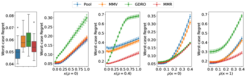
Figure 6.1: Left: the worst-case regret on the testing data without data perturbation ($\kappa=0$ and $\rho=0$). Right four panels: the worst-case regret under various data perturbation designs.

6.2 Results

We compare the proposed MMR method with the pooled ERM, GDRO, and MMV methods in terms of robustness against the above data perturbations. Specifically, we reserve $100$ random samples per group for testing and use the remaining samples for training. To evaluate prediction performance, we report the average worst-case regret on the test set over $30$ replicates. As shown on the left side of Figure 6.1, four methods achieve comparable worst-case regrets on the original data ($\rho=0$ and $\kappa=0$), while the pooled estimate performs slightly better. As we increase the magnitude of heterogeneity in measurement errors or potential effect modification, the proposed MMR method consistently achieves a performance comparable to or superior to that of the other three methods. The top right of Figure 6.1 indicates that the GDRO method is particularly sensitive to increases in the disparity of Bayes risks between groups. The rate at which the worst-case regret increases for the GDRO estimate is markedly faster than that for the other three estimates. In addition, as shown on the bottom right of Figure 6.1, when the effect modification on one group increases (i.e., when $\rho$ gets larger), the performances of the pooled and MMV estimators decrease considerably. Overall, the MMR method demonstrates uniform performance across different groups through the worst-group regret guarantee. In particular, our MMR method has better adaptability to various data qualities and latent effect modifiers among transplant centers than the other three methods.

7 Summary

In this work, we have introduced a general min-max-regret (MMR) learning framework. We aim to improve the model robustness and generalizability across heterogeneous sub-populations under the regret criterion. In the context of linear regression, our robust regret-based method can achieve several robustness and invariance properties simultaneously, including the group proportion invariance, heteroscedasticity invariance, as well as the regression equivariance. We have also investigated the MMR problem and its duality for linear regression, which sheds lights on its geometric characterization (solving the minimal bounding ellipsoid problem), the worst-case sub-populations that support the estimator, and the attraction to regret parity in its dual problem. Moreover, we have established the generalizability guarantees on the worst-case regret over both of the observed sub-populations and the unseen ones from a super-population. This is particularly useful when the training data involve a large number of groups “sampled” for meta analysis.

There are several future directions to be explored based on the proposed framework. In this work, we consider MMR in the context of supervised learning. It would be interesting to employ the MMR framework in other problem setups. For example, it could be extended to learning optimal treatment regimes in precision medicine and the development of robust policies in statistical decision making [25]. In addition, our proposed algorithm focuses on a general smoothed and strongly convex loss. Another interesting direction is to develop algorithms for non-smooth, non-convex losses, such as the zero-one loss in classification. These extensions would further broaden the applicability of the MMR framework.

References

- [1] Alekh Agarwal and Tong Zhang “Minimax Regret Optimization for Robust Machine Learning under Distribution Shift” In Proceedings of the 35th Conference on Learning Theory, 2022, pp. 2704–2729
- [2] Peter L Bartlett, Olivier Bousquet and Shahar Mendelson “Local rademacher complexities” In The Annals of Statistics 33.4, 2005, pp. 1497–1537
- [3] Su Lin Blodgett, Lisa Green and Brendan O’Connor “Demographic Dialectal Variation in Social Media: A Case Study of African-American English” In Proceedings of the 2016 Conference on Empirical Methods in Natural Language Processing, 2016, pp. 1119–1130 DOI: 10.18653/v1/D16-1120
- [4] Daniel Cer, Mona Diab, Eneko Agirre, Iñigo Lopez-Gazpio and Lucia Specia “SemEval-2017 Task 1: Semantic Textual Similarity Multilingual and Crosslingual Focused Evaluation” In Proceedings of the 11th International Workshop on Semantic Evaluation, 2017, pp. 1–14 DOI: 10.18653/v1/S17-2001
- [5] Yifan Cui “Individualized decision-making under partial identification: Three perspectives, two optimality results, and one paradox” In Harvard Data Science Review 3.3, 2021, pp. 1–19
- [6] Laurens de Haan and Ana Ferreira “Extreme Value Theory: An Introduction” Springer New York, 2006
- [7] Jeff Dominitz and Charles F Manski “Minimax-regret sample design in anticipation of missing data, with application to panel data” In Journal of Econometrics 226.1 Elsevier, 2022, pp. 104–114
- [8] Jeff Dominitz and Charles Manski F “More data or better data? A statistical decision problem” In The Review of Economic Studies 84.4 Oxford University Press, 2017, pp. 1583–1605
- [9] Cynthia Dwork, Moritz Hardt, Toniann Pitassi, Omer Reingold and Richard Zemel “Fairness through awareness” In Proceedings of the 3rd Innovations in Theoretical Computer Science Conference, 2012, pp. 214–226
- [10] Damian Gola, Jeanette Erdmann, Kristi Läll, Reedik Mägi, Bertram Müller-Myhsok, Heribert Schunkert and Inke R König “Population bias in polygenic risk prediction models for coronary artery disease” In Circulation: Genomic and Precision Medicine 13.6 Am Heart Assoc, 2020, pp. e002932
- [11] Zijian Guo “Statistical inference for maximin effects: Identifying stable associations across multiple studies” To appear In Journal of the American Statistical Association Taylor & Francis, 2023
- [12] Weihua Hu, Gang Niu, Issei Sato and Masashi Sugiyama “Does Distributionally Robust Supervised Learning Give Robust Classifiers?” In Proceedings of the 35th International Conference on Machine Learning 80, 2018, pp. 2029–2037 URL: https://proceedings.mlr.press/v80/hu18a.html
- [13] Mia Hubert, Peter J Rousseeuw and Stefan Aelst “High-Breakdown Robust Multivariate Methods” In Statistical Science 23.1 JSTOR, 2008, pp. 92–119
- [14] Takuya Ishihara and Toru Kitagawa “Evidence aggregation for treatment choice” In arXiv preprint arXiv:2108.06473, 2021
- [15] W James and Charles Stein “Estimation with Quadratic Loss” In Proceedings of the 4th Berkeley Symposium on Mathematical Statistics and Probability, 1961, pp. 361–379
- [16] Pang Wei Koh, Shiori Sagawa, Henrik Marklund, Sang Michael Xie, Marvin Zhang and Akshay Balsubramani “WILDS: A Benchmark of in-the-Wild Distribution Shifts” In Proceedings of the 38th International Conference on Machine Learning, 2021, pp. 5637–5664
- [17] Lihua Lei, Roshni Sahoo and Stefan Wager “Policy Learning under Biased Sample Selection” In arXiv preprint arXiv:2304.11735, 2023
- [18] Amy Lewis, Angeliki Koukoura, Georgios-Ioannis Tsianos, Athanasios Apostolos Gargavanis, Anne Ahlmann Nielsen and Efstathios Vassiliadis “Organ donation in the US and Europe: The supply vs demand imbalance” In Transplantation Reviews 35.2, 2021, pp. 100585 DOI: https://doi.org/10.1016/j.trre.2020.100585
- [19] Hongyang Li, Daniel Quang and Yuanfang Guan “Anchor: Trans-cell type prediction of transcription factor binding sites” In Genome research 29.2 Cold Spring Harbor Lab, 2019, pp. 281–292
- [20] Charles F Manski “Econometrics for decision making: Building foundations sketched by haavelmo and wald” In Econometrica 89.6 Wiley Online Library, 2021, pp. 2827–2853
- [21] Charles F Manski “Statistical treatment rules for heterogeneous populations” In Econometrica 72.4 Wiley Online Library, 2004, pp. 1221–1246
- [22] Pascal Massart “Some applications of concentration inequalities to statistics” In Annales de la Faculté des sciences de Toulouse 9.2, 2000, pp. 245–303
- [23] Nicolai Meinshausen and Peter Bühlmann “Maximin effects in inhomogeneous large-scale data” In The Annals of Statistics 43.4 Institute of Mathematical Statistics, 2015, pp. 1801–1830
- [24] Lamine Mili and Clint W Coakley “Robust estimation in structured linear regression” In The Annals of Statistics 24.6 Institute of Mathematical Statistics, 1996, pp. 2593–2607
- [25] Weibin Mo, Zhengling Qi and Yufeng Liu “Learning optimal distributionally robust individualized treatment rules” In Journal of the American Statistical Association 116.534 Taylor & Francis, 2021, pp. 659–674
- [26] National Academies of Sciences, Engineering, and Medicine “The state of health disparities in the United States” In Communities in Action: Pathways to Health Equity, 2017, pp. 57–97
- [27] Yurii Nesterov “Lectures on Convex Optimization” Springer Cham, 2018
- [28] Bret Nestor, Matthew BA McDermott, Willie Boag, Gabriela Berner, Tristan Naumann, Michael C Hughes, Anna Goldenberg and Marzyeh Ghassemi “Feature robustness in non-stationary health records: Caveats to deployable model performance in common clinical machine learning tasks” In Machine Learning for Healthcare Conference, 2019, pp. 381–405
- [29] Hamed Rahimian and Sanjay Mehrotra “Distributionally robust optimization: A review” In arXiv preprint arXiv:1908.05659, 2019
- [30] Ralph Tyrell Rockafellar “Convex Analysis” Princeton University Press, 1970 DOI: doi:10.1515/9781400873173
- [31] Peter J Rousseeuw and Annick M Leroy “Robust regression and outlier detection” John Wiley & Sons, 1987
- [32] Shiori Sagawa, Pang Wei Koh, Tatsunori B Hashimoto and Percy Liang “Distributionally robust neural networks for group shifts: On the importance of regularization for worst-case generalization” In arXiv preprint arXiv:1911.08731, 2019
- [33] Rajiv Saran, Bruce Robinson, Kevin C Abbott, Lawrence YC Agodoa, Jennifer Bragg-Gresham and Rajesh Balkrishnan “US renal data system 2016 annual data report: Epidemiology of kidney disease in the United States” In American Journal of Kidney Diseases 65.5 Elsevier, 2017, pp. A7–A8
- [34] Leonard J Savage “The theory of statistical decision” In Journal of the American Statistical Association 46.253 Taylor & Francis, 1951, pp. 55–67
- [35] Harvineet Singh, Vishwali Mhasawade and Rumi Chunara “Generalizability challenges of mortality risk prediction models: A retrospective analysis on a multi-center database” In PLoS Digital Health 1.4 Public Library of Science San Francisco, CA USA, 2022, pp. e0000023
- [36] Rachael Tatman “Gender and Dialect Bias in YouTube’s Automatic Captions” In Proceedings of the 1st ACL Workshop on Ethics in NLP, 2017, pp. 53–59 DOI: 10.18653/v1/W17-1606
- [37] Robert Tibshirani “Regression shrinkage and selection via the lasso” In Journal of the Royal Statistical Society Series B: Statistical Methodology 58.1 Oxford University Press, 1996, pp. 267–288
- [38] John R Zech, Marcus A Badgeley, Manway Liu, Anthony B Costa, Joseph J Titano and Eric Karl Oermann “Variable generalization performance of a deep learning model to detect pneumonia in chest radiographs: A cross-sectional study” In PLoS Medicine 15.11 Public Library of Science San Francisco, CA USA, 2018, pp. e1002683