Privacy-aware Berrut Approximated Coded Computing for Federated Learning

Abstract

Federated Learning (FL) is an interesting strategy that enables the collaborative training of an AI model among different data owners without revealing their private datasets. Even so, FL has some privacy vulnerabilities that have been tried to be overcome by applying some techniques like Differential Privacy (DP), Homomorphic Encryption (HE), or Secure Multi-Party Computation (SMPC). However, these techniques have some important drawbacks that might narrow their range of application: problems to work with non-linear functions and to operate large matrix multiplications and high communication and computational costs to manage semi-honest nodes. In this context, we propose a solution to guarantee privacy in FL schemes that simultaneously solves the previously mentioned problems. Our proposal is based on the Berrut Approximated Coded Computing, a technique from the Coded Distributed Computing paradigm, adapted to a Secret Sharing configuration, to provide input privacy to FL in a scalable way. It can be applied for computing non-linear functions and treats the special case of distributed matrix multiplication, a key primitive at the core of many automated learning tasks. Because of these characteristics, it could be applied in a wide range of FL scenarios, since it is independent of the machine learning models or aggregation algorithms used in the FL scheme. We provide analysis of the achieve privacy and complexity of our solution and, due to the extensive numerical results performed, it can be observed a good trade-off between privacy and precision.

I Introduction

Federated Learning (FL) [1] emerged as an adequate strategy to support collaborative training of AI models without sharing private data. The philosophy is not complex: (i) each worker node (or data owner) trains a local version of the AI model using its own private data; (ii) then, it shares the model (parameter, gradients, etc., depending on the AI algorithm) with a central computation node (or aggregator) which is in charge of (iii) assembling a global model, i.e. combining the partial knowledge of each node to obtain a global knowledge; and finally, (iv) sharing the global model with all the worker nodes in the collaborative (federated) network. This process is repeated until the global model converges. Despite its apparent simplicity, there are important challenges that arise in this new FL schemes, such as overheads in communication, management of non identically distributed computational resources and/or data, identification of suitable techniques to aggregate different models or privacy leaks because of the exchange of the AI models information.

In this paper, we exclusively focus on the privacy concerns that have been highlighted in the literature [2, 3], such as the possibility of membership inference attacks [4, 5], inferring class representatives [6], inferring properties [7] or even being able to reconstruct the original data by inverting gradients [8]. These concerns have led to the emergence of different privacy enhancing technologies (PET) focused on trying to avoid privacy leaks [9], being the most used strategies the following ones:

1. Differential privacy (DP) [10] adds noise to the dataset before being locally used in the training stage, but it requires a high precision loss in order to achieve high privacy requirements.

2. Homomorphic encryption (HE) [11] performs computations directly on the encrypted domain, but it requires high computation resources and it is difficult to apply with non-linear functions.

3. Secure Multi-Party Computation (SMPC) [12], closely related to the problem of secret sharing, allows a group of nodes to collaboratively compute a function over an input while keeping it secret. It entails high communication overheads and it cannot generally handle non-linear functions.

However, these techniques have also some drawbacks. First, when dealing with semi-honest nodes, it is needed to add additional strategies to neutralize their behaviour, which increases the communication and computational costs and it would finally have a high impact in the scalability of the FL system [13].

Besides, and since HE and SMPC are not suitable to deal with non-linear functions, the application of these techniques may narrow the range of AI models and aggregation algorithms used in FL schemes [14]. This would entail, first, usability implications, since there are AI models that cannot be applied in specific fields [15, 16] and second, security implications, since some robust aggregation algorithms to deal with malicious nodes cannot be used [17, 18]. Additionally to the non-linear issues, managing matrix multiplications, which is needed in different AI algorithms, requires from high computation resources, aspect that has been addressed in the literature [19, 20, 21].

Within this context, we propose to face the problem from the perspective of a large-scale distributed computing system, since FL naturally matches this scheme: a complex computation (global learning model) is distributedly performed by several worker nodes. Anyway, large-scale distributed computing systems have to deal with two important issues: communication overheads and straggling nodes. The former is due to the exchange of intermediate results in order to be able to collaboratively obtain the final one. The latter is due to slow worker nodes that reduce the runtime of the whole computation. Preciselly, the Coded Distributed Computing (CDC) paradigm [22, 23] arose to reduce both problems by combining coding techniques and redundant computation approaches. However, the CDC techniques cannot simultaneously guarantee privacy and work with non-linear functions. Besides, CDC schemes are usually applied for decentralized computations (one master node and one input dataset), but for FL (multiple datasets) it is more appropriate to work with a scheme like secret sharing protocols [24, 25], whose most famous approach is the Shamir Secret Sharing (SSS) [26]. In this context, we propose a CDC-based solution with the following contributions:

• A CDC solution able to guarantee privacy and also able to manage non-linear functions. Recently, a CDC approach, the Berrut Approximated Coded Computing (BACC) [27], was proposed to manage non-linear function in large distributed computation architectures. Thus, our first contribution defines a computation scheme that adds input privacy to the BACC algorithm, which we have coined as Privacy-aware Berrut Approximated Coded Computing (PBACC) scheme. In order to check the privacy-precision cost, We have performed a theoretical analysis of the privacy in PBACC.

• Extend the PBACC scheme to a multi-input secret sharing configuration, suitable for FL scenarios. Thus, our second contribution, coined as Private BACC Secret Sharing (PBSS), is based on the Shamir Secret Sharing, but assuring a secure FL aggregation process. We have also performed a theoretical analysis of the computational complexity of PBSS.

• Adapt the PBACC scheme to support optimized secure matrix multiplication. Due to the coding process, PBACC introduces additional computational load when multiplying matrices. Thus, our third contribution focuses on providing an appropriate multiplication mechanism that allows large matrix multiplication with three improvements: privacy-awareness, block partition and simultaneous encoding. We have also performed a theoretical analysis of the achieved privacy and a complexity analysis of our proposal.

In order to validate our proposal (PBSS), we have performed different experiments in FL settings to compare its behaviour in presence of stragglers with the original BACC with secret sharing without privacy. We have compared the precision of both schemes when dealing with non-linear functions and complex matrix multiplications. More specifically, we have performed experiments with three typical activation functions in machine learning algorithms (ReLU, Sigmoid and Swish) and two typical non-linear aggregation methods to combine learning models (Binary Step and Median) [14]. Besides, we have checked the performance of our proposal (PBSS) when operating complex matrices. In all cases the results are really promising, since the cost of adding privacy even in presence of stragglers is not significant in terms of precision.

The rest of the paper is organized as follows. Section II briefly reviews some relevant works related to our proposal, and includes a description of the BACC approach [27]. Section III describes our first contribution PBACC and includes an analysis of the achieved privacy. In Section IV, we detail how to extend PBACC to a multi-input secret sharing setting (PBSS) and the analysis its computational complexity. In Section V we detail our contribution to extend our scheme for matrix multiplication, including the privacy and complexity analysis. In Section VI we test our proposal and, finally, Section VII summarizes the main conclusions of this work, and outlines some future work.

II Related Work

Coded distributed computing (CDC) techniques  [28, 22, 23] combine coding theory and distributed computing to alleviate the two main problems in large distributed computation. First, the high communication load due to the exchange of intermediate operations. This has been applied, for instance, in [29] for data shuffling, reducing communication bottlenecks by exploiting the excess in storage (redundancy). Second, the delay due to straggling nodes, which has been used in MapReduce schemes, for instance, to encode Map tasks even when not all the nodes had finished their computations [30].

Private Coded Distributed Computing (PCDC) [31] is a subset of Coded Distributed Computing (CDC) that focuses on preserving privacy of input data. Generally speaking, PCDC approaches try to compute a function among a set of distributed nodes but keeping the input data in secret. Thus, a central element divides the data into coded pieces that are shared with the computation nodes. Computation nodes, then, apply the goal function on these pieces of information (also known as shares). These partial results are, finally, sent to the central element to build the final result. The main research challenge in PCDC is trying to reduce the number of nodes that are required to carry out the computation of a given function.

One remarkable approach in the PCDC field is the Lagrange Coded Computing (LCC) [32], which has been proposed as a unified solution for computing general multivariate polynomials (goal function) by using the Lagrange interpolation polynomial to create computation redundancy. LCC is resilient against stragglers, secure against malicious (Byzantine) nodes and adds privacy to the data set. Besides, and compare to other previous approaches, LCC reduces storage needs as well as reduces the communication and randomness overhead. However, LCC also has some important limitations: (i) it does not work with non-linear functions, (ii) it is numerically unstable when the input data are rational numbers or when the number of nodes is too large, and (iii) it relies on quantizing the input into the finite field. With the aim of overcoming the last of them, an extension of LCC for the analog domain was recently proposed [33]: Analog LCC (ALCC). However, it cannot solve the other issues related to the Lagrange interpolation.

The Berrut Approximated Coded Computing (BACC) [27] offers a solution to the LCC or ALCC previously mentioned issues. BACC approximately computes arbitrary goal functions (not only polynomials) by dividing the calculus into an arbitrary large number of nodes (workers). The error of the approximation was theoretically proven to be bounded. However, BACC does not include any privacy guarantee.

All the previously mentioned CDC schemes are suitable for computations with one master node and one input data set. In FL settings, where there are multiple input data sets, one per node (worker), it would be more adequate to use the philosophy of the polynomial sharing approach [34], based on the Shamir Secret sharing (SSS) [26] approach. In SSS the private information (secret) is split up in parts or shares, which are sent to the workers. The secret cannot be reassembled unless a sufficient number of nodes work together to reconstruct the original information.

Related to this last issue within SMPC, emerges the recurring problem of multiplying large matrices in a scalable and secure way. It is specially difficult to reduce communication and computation overheads (scalability) while maintaining privacy in the data and, besides, being resilient to stragglers. There are some approaches in the literature to face these issues, like  [34], which proposes a method for secure computation of massive matrix multiplication offloading the task to clusters of workers, or [35], a scheme for secure matrix multiplication in presence of colluding nodes.  [36] proposes entangled polynomial codes to break the cubic barrier of the recovery threshold for batch distributed matrix multiplications and [37] proposes a coding scheme for batch distributed matrix multiplication resistant to stragglers.

III PBACC: Berrut Approximated Coded Computing with Privacy

As previously mentioned, we have selected the Berrut Approximated Coded Computing (BACC) [27] as our building block for distributed computing because it works with non-linear computations, it is numerically stable, and has a lower computational complexity. However, BACC does not offer privacy guarantees, which is the issue we solved with our first contribution PBACC. In presence of colluding nodes, we define the privacy leakage of the scheme as the mutual information between the data and the messages captured by the curious nodes. This mutual information can be upper bounded by the value of the Shannon capacity of an equivalent MIMO channel.

III-A Preliminaries

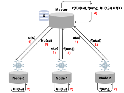
Figure 1: Decentralized computation of a function using BACC for 3 nodes.

Given an arbitrary matrix function $f:\mathbb{V}\rightarrow\mathbb{U}$ over some input data $\mathbf{X}=(X_{0},\dots,X_{K-1})$, where $\mathbb{U}$ and $\mathbb{V}$ are vector spaces of real matrices, BACC performs the approximate evaluation of $f(\mathbf{X})=\bigl{(}f(X_{1}),\dots,f(X_{K-1})\bigr{)}$, where $X_{i}\in\mathbb{V}$, in a numerically stable form and with a bounded error. The computation is executed in a decentralized configuration with one master node, who owns the data, and $N$ worker nodes in charge of computing $f(\cdot)$ at some interpolation points which encode $\mathbf{X}$ in a form that prevents the workers to learn much information about the data. The general procedure is depicted in Fig. 1, and explained next.

III-A1 Encoding and Sharing

To perform the encoding of the input data $\mathbf{X}$, the following rational function $u:\mathbb{C}\rightarrow\mathbb{V}$ is composed by the master node

$$u(z)=\sum_{i=0}^{K-1}\frac{\frac{(-1)^{i}}{(z-\alpha_{i})}}{\sum_{j=0}^{K-1}\frac{(-1)^{j}}{(z-\alpha_{j})}}X_{i},$$ (1)

for some distinct points $\boldsymbol{\alpha}=(\alpha_{0},\dots,\alpha_{K-1})\in\mathbb{R}^{K}$. By definition, it is easy to verify that $u(\alpha_{j})=X_{j}$, for $j\in\{0,\dots,K-1\}$. In the original BACC, it is suggested to choose the interpolation points $\boldsymbol{\alpha}$ as the Chebyshev points of first kind $\alpha_{j}=\operatorname{Re}(e^{\imath(2j+1)\pi/(2K)})$ where $\imath=\sqrt{-1}$. Then, the master node selects $N$ points $\{z_{j}:j=0,\dots,N-1\}$, computes $u(z_{j})$, and assigns this value to worker $j$. In [27], it is suggested to choose $\{z_{j}:j=0,\dots,N-1\}$ as the Chebyshev points of second kind $z_{j}=\operatorname{Re}(e^{\imath j\pi/(N-1)})$.

III-A2 Computation

Upon receiving $u(z_{j})$, worker $j$ computes $v_{j}=f\bigl{(}u(z_{j})\bigr{)}$.

III-A3 Communication

Worker $j$ sends the result $v_{j}$ to the master node.

III-A4 Decoding and recovery

When the master collects $n\leq N$ results from the subset $\mathcal{F}$ of fastest nodes, it approximately calculates $f(X_{j})$, for $j=\{0,\dots,K-1\}$, using the decoding function based on the Berrut rational interpolation

$$r_{\mathrm{Berrut},\mathcal{F}}(z)=\sum_{i=0}^{n}\frac{\frac{(-1)^{i}}{(z-\tilde{z}_{i})}}{\sum_{j=0}^{n}\frac{(-1)^{j}}{(z-\tilde{z}_{j})}}f(u(\tilde{z}_{i})),$$

where $\tilde{z}_{i}\in\mathcal{S}$ are the interpolation points $\mathcal{S}=\{\cos\frac{j\pi}{N-1},j\in\mathcal{F}\}$ from the $n$ faster nodes. At this moment, the master node computes the approximation $f(X_{i})\approx r_{\mathrm{Berrut},\mathcal{F}}(\alpha_{i})$, for $i\in\{0,\dots,K-1\}$.

III-B PBACC: Adding privacy to BACC

As explained, the original BACC distributed computing solution is based on the rational interpolation function (1) and the choice of $\boldsymbol{\alpha}$ as interpolation points, so that $u(\alpha_{i})=X_{i}$ for all $i$. For the purpose of adding privacy, and similar to other works [38, 39], we introduce $T$ random coefficients into the encoding function, where $T$ is a design parameter. The encoding function is now

$$w(z) =\sum_{i=0}^{K-1}\frac{\frac{(-1)^{j}}{(z-\alpha_{i})}}{\sum_{j=0}^{K+T-1}\frac{(-1)^{j}}{(z-\alpha_{j})}}X_{i}+\sum_{i=0}^{T-1}\frac{\frac{(-1)^{K+i}}{(z-\alpha_{K+i})}}{\sum_{j=0}^{K+T-1}\frac{(-1)^{j}}{(z-\alpha_{j})}}R_{i}$$ (2)

$$=\sum_{i=0}^{K+T-1}\frac{\frac{(-1)^{j}}{(z-\alpha_{i})}}{\sum_{j=0}^{K+T-1}\frac{(-1)^{j}}{(z-\alpha_{j})}}W_{i},$$

where $\mathbf{W}=(X_{0},\dots,X_{K-1},R_{0},\dots,R_{T-1})=(W_{0},\dots,W_{K+T-1})$. Here, $\{R_{0}:i=1,\dots,T-1\}$ are random data points independently generated according to a given distribution $\mathcal{G}$ to be specified later. To be able to accomplish the interpolation of the values of $f(X_{i})$ for all $i$, we propose to select as interpolation points, the Chebyshev points of first kind, and as evaluation points the shifted points $\beta_{j}=b+\alpha_{j}=b+\operatorname{Re}(e^{\imath(2j+1)\pi/(2T)})$ where $b\in\mathbb{R}$, for $j=0,\dots,T-1$. Clearly, adding the randomness coefficients in (2) does not modify the identities $w(\alpha_{i})=X_{i}$ for $0\leq i<K$. The proposed scheme will be referred to as Privacy-aware Berrut Approximated Coded Computing (PBACC) hereafter.

III-C Measuring the privacy of PBACC

Our focus is this paper is not on perfect information-theoretical privacy, where the adversaries cannot learn anything about the local data sets of honest clients, but on bounded information leakage. Therefore, similar to other works [33, 40], we use the mutual information $I(\mathbf{X};\mathbf{Y})$, which is a measure of the statistical correlation of two random variables $\mathbf{X}$ and $\mathbf{Y}$, as the privacy leakage metric. One of the variables $\mathbf{X}$ will correspond to the private input, while the other $\mathbf{Y}$ will represent the encoded output, and is a worst-case for the information accessible to the curious or semi-honest colluding nodes. Specifically, we assume that, in our system, up to $T$ nodes can be honest but curious, or semi-honest in short. This means that these nodes, whose identities are unknown to the remaining honest nodes, can attempt to disclose information on the private data $\mathbf{X}$ by means of observation $\mathbf{Y}$ of the encoded information and direct message exchange among them. Notice that semi-honest nodes respect the computation protocol, i.e., they do not inject malicious or malformed messages to deceive the master node.

Generally, the exact computation of $I(\mathbf{X};\mathbf{Y})$ under the described threat model is not feasible. Instead, since our goal is to obtain a bounded leakage assurance, we leverage the existent results about the capacity of a Multi-Input Multi-Output (MIMO) channel under some specific constraints [41], to bound the mutual information, using similar techniques to [33]. Such bound is based in the fact that a MIMO channel with $K$ transmitter antennas and $T$ receiver antennas is, conceptually from an information-theoretic perspective, equivalent to a signal composed of the $K$ encoded elements of the input in BACC, and an observation cooperatively formed by the $T$ colluding nodes, which collect and possibly process these encoded messages to infer information about the data. In this configuration, the encoded noise of the channel acts as the element that provides security, since it reduces the amount of information received by the colluding nodes. We assume for the analysis that follows that the noise is Gaussian (so the channel is an AWGN vector channel).

Now, for this privacy analysis, we start with the encoding function (2), written as $w(z)=\sum_{i=0}^{K-1}X_{i}q_{i}(z)+\sum_{i=K}^{K+T-1}R_{i-K}q_{i}(z)$, where

$$q_{i}(z)=\frac{\frac{(-1)^{i}}{(z-\alpha_{i})}}{\sum_{j=0}^{K+T-1}\frac{(-1)^{j}}{(z-\alpha_{j})}}$$

is one of the rational interpolating terms. Without loss of generality, we assume that each entry of $X_{i}$ is a realization of a random variable with a distribution supported in the interval $D_{s}\triangleq[-s,s]$, for all $i=\{0,\dots,K-1\}$, and that the random coefficients $R_{i}\sim\mathcal{N}(0,\frac{\sigma_{n}^{2}}{T})$, where $\mathcal{N}(0,a)$ denotes the Gaussian distribution with zero mean and variance $a$. Note that, having a finite support $D_{s}$, $X_{i}$ has finite power. If we denote $\mathbf{Y}=(w(z_{i_{1}}),w(z_{i_{2}}),\dots,w(z_{i_{T}}))^{T}$, for the messages observed by the $T$ colluding adversaries $\mathcal{T}=\{i_{1},i_{2},\dots,i_{T}\}$, where $z_{i_{h}}$ are some of the Chebyshev points of second kind, we can write

$$\mathbf{Y}=Q_{T}\mathbf{X}+\tilde{Q}_{T}\mathbf{R},$$ (3)

where the matrices $Q_{T}$ and $\tilde{Q}_{T}$ are given by

$$Q_{T}\triangleq\begin{pmatrix}q_{0}(z_{i_{1}})&\ldots&q_{K-1}(z_{i_{1}})\\ q_{0}(z_{i_{2}})&\ldots&q_{K-1}(z_{i_{2}})\\ \vdots&\ddots&\vdots\\ q_{0}(z_{i_{T}})&\ldots&q_{K-1}(z_{i_{T}})\end{pmatrix}_{T\times K},$$

$$\tilde{Q}_{T}\triangleq\begin{pmatrix}q_{K}(z_{i_{1}})&\ldots&q_{K+T-1}(z_{i_{1}})\\ q_{K}(z_{i_{2}})&\ldots&q_{K+T-1}(z_{i_{2}})\\ \vdots&\ddots&\vdots\\ q_{K}(z_{i_{T}})&\ldots&q_{K+T-1}(z_{i_{T}})\end{pmatrix}_{T\times T}.$$

The amount of information revealed to $\mathcal{T}$ —the information leakage $I_{L}$— is defined in this work as the worst-case achievable mutual information for the colluding nodes [40]

$$I_{L}\triangleq\max_{\mathcal{T}}\sup_{P_{\mathbf{X}}:|X_{i}|\leq s|,\forall i\in[K]}I(\mathbf{Y};\mathbf{X}),$$

where $P_{\mathbf{X}}$ is the probability density function of $\mathbf{X}$, and the maximization applies to any $\mathcal{T}\subset[N]$. As $\|X_{i}\|\leq s$, this implies that the power $\mathbb{E}[\|X_{i}\|]^{2}\leq s^{2}$. Therefore, the latter equation can be re-written as

$$I_{L}\leq\max_{\mathcal{T}}\sup_{P_{\mathbf{X}}:\mathbb{E}[\|X_{i}\|^{2}]\leq s^{2}}I(\mathbf{Y};\mathbf{X}).$$ (4)

In order to bound $I_{L}$, since the noise used for privacy in BACC is Gaussian, we consider an equivalent formulation of (3) as a MIMO channel with $K$ transmitter antennas and $T$ receiver antennas, so the input-output relation can be defined as

$$\mathbf{Y}=H\mathbf{X}+\mathbf{Z},$$

where $H_{T\times K}$ is the channel gain matrix known by both transmitter and receiver, and $\mathbf{Z}_{T\times 1}$ is a vector of additive Gaussian noise with 0 mean. Further, let us denote the covariance matrix of the vector $\mathbf{Z}$ as $\Sigma_{\mathbf{Z}}$. Using known results on the capacity of a MIMO channel with the same power allocation constraint and correlated noise [41],

$$C=\sup_{P_{\mathbf{X}}}I(\mathbf{Y};\mathbf{X})=\log_{2}|I_{T}+PH\Sigma^{-1}_{\mathbf{Z}}H^{\dagger}|,$$

where $P$ is the maximum power of each transmitter antenna, $I_{T}$ is the identity matrix of order $T$ and $|\cdot|$ is the determinant of a matrix. Thus, using (4) and assuming that the noise is uncorrelated, we have

$$\ I_{L}\leq\max_{\mathcal{T}}\log_{2}\bigl{|}I_{T}+\frac{s^{2}T}{\sigma^{2}_{n}}\tilde{\Sigma}_{T}^{-1}\Sigma_{T}\bigr{|},$$

where $\tilde{\Sigma}_{T}\triangleq\tilde{Q}_{T}\tilde{Q}_{T}^{\dagger}$ and $\Sigma_{T}\triangleq Q_{T}Q_{T}^{\dagger}$.

Since the information leakage grows with $K$, the privacy metric $\imath_{L}$ of BACC is defined in this paper as the normalized value of $I_{L}$, namely $\imath_{L}=\frac{I_{L}}{K}$, and we will say that BACC has $\epsilon$-privacy if $\imath_{L}<\epsilon$, where $\epsilon>0$ is the target security parameter of the scheme and represents the maximum amount of leaked information per data point that is allowed for a fixed number of colluding nodes $T$. The value of this parameter will strongly depend on the specific ML model or application under consideration at each case.

IV PBSS: PBACC with Secret Sharing

While PBACC provides quantifiable privacy for distributed computations, it is not yet valid for FL, since it only supports a single data owner (the master). The workers are just delegated nodes for the computation tasks. In contrast, in FL the roles are reversed: the clients perform local training and are also the data owners, whereas the aggregator node is the central entity doing the model aggregation. Therefore, to be useful for general FL frameworks, PBACC needs to be enhanced to a multi-input secret sharing configuration, one that allows a set of nodes to collaboratively compute a function, either training or aggregation, whose final results can be decoded by the central aggregator. After the protocol is defined, it is also essential to measure its communication and computation costs in each phase, so that it proves scalable in addition to privacy-preserving. In the following, the Private BACC Secret Sharing (PBSS) protocol is presented (Section IV-A), and its computational complexity is analyzed (Section IV-B).

IV-A Private BACC Secret Sharing (PBSS) protocol

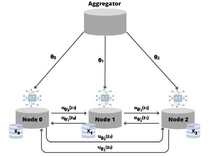
(a) Phase 1 of PBSS- Sharing.

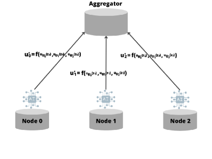
(b) Phase 2 of PBSS - Computation and communication.

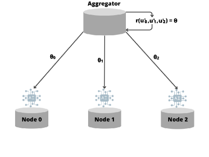
(c) Phase 3 of PBSS - Reconstruction phase.

Figure 2: PBSS phases

Suppose a collection of $N$ nodes, each one having a private data vector $\mathbf{X}^{(i)}=\begin{pmatrix}X_{0}^{(i)}&\ldots&X_{K-1}^{(i)}\end{pmatrix}^{T}$, where the input data $\mathbf{X}^{(i)}\in\mathbb{R}^{K\times L}$ is owned by node $i$, for $i\in\{0,\dots,N-1\}$. The PBSS consists of three phases, that are detiled as follows:

Phase 1 - Sharing: The first phase is based on classical Shamir Secret Sharing [26]. The client node $i$ composes the following encoded polynomial quotient

$$v_{\mathbf{X}^{(i)}}(z) =\sum_{j=0}^{K-1}\frac{\frac{(-1)^{j}}{(z-\alpha_{j})}}{\sum_{k=0}^{K+T-1}\frac{(-1)^{k}}{(z-\alpha_{k})}}X_{j}^{(i)}$$ (5)

$$+\sum_{j=0}^{T-1}\frac{\frac{(-1)^{j+K}}{(z-\alpha_{j})}}{\sum_{k=0}^{K+T-1}\frac{(-1)^{j}}{(z-\alpha_{k})}}R_{j}^{(i)},$$

for some distinct interpolation points associated to the the data $\mathbf{X}^{(i)}$, $\boldsymbol{\alpha}=(\alpha_{0},\dots,\alpha_{K-1})\in\mathbb{R}^{K}$, which we choose again as the Chebyshev points of first kind $\alpha_{j}=\cos\left(\frac{(2j+1)\pi}{2K}\right)$, and some distinct interpolation points associated to the $R^{(i)}_{j}$, $\alpha_{K},\dots,\alpha_{K+T-1}\in\mathbb{R}$, which are selected as the shifted Chebyshev points of first kind $\alpha_{K+j}=b+\cos\left(\frac{(2j+1)\pi}{2K}\right)$. The rational function $v_{\mathbf{X}^{(i)}}(z)$ is evaluated at the set $\{z_{j}\}$, for $j=0,\dots,N-1$, using $z_{j}=\cos(\frac{j\pi}{N-1})$, the Chebyshev points of second kind. Finally, the random coefficients $R_{j}^{(i)}$ are distinct $1\times L$ vectors drawn from a Gaussian distribution $\mathcal{N}(0,\frac{\sigma_{n}^{2}}{T})$. The evaluation $v_{\mathbf{X}^{(i)}}(z_{j})$ is the share created from the client node $i$ and sent to the node $j$, as explained below. The sharing phase is represented in Fig. 2a assuming there are three workers owning their own private data set ($X_{j}$) and locally computing a local AI model. As it is shown, the aggregator sends the global model ($\theta$) to the nodes, so they can complete a new round of their learning task. The parameters of the global model are codified, using the function $u()$ established in eq. (5), and shared with the three nodes. After this codification part, the PBSS scheme acts: each node $j$ receives the shares created using the evaluation point $z_{j}$, and computes the aggregation function $f()$ over the codified parameters $u_{\theta^{\prime}_{i}}(z_{j})$. In this case, the input data to be secured for the node $i$ is $\theta^{\prime}_{i}$, the model updates after the local computation is done.

Phase 2 - Computation and communication: In this phase, the node $i$ calculates an arbitrary function $f$ using a set of polynomial quotient evaluations shared from the rest of nodes $\{v_{\mathbf{X}^{(0)}}(z_{i}),u_{\mathbf{X}^{(1)}}(z_{i}),\dots,u_{\mathbf{X}^{(N-1)}}(z_{i})\}$, where $u_{\mathbf{X}^{(j)}}(z_{i})$ is the evaluation of the rational function corresponding to the input $X^{(j)}$ owned by the $j$-th node, and shared with node $i$. The client node $i$ computes $f\bigl{(}v_{\mathbf{X}^{(j)}}(z_{i})\bigr{)},\quad j=\{0,\dots,N-1\}$ and sends the result to the master node. This phase is schematically represented in Fig. 2b, where the obtained results $f(u_{\theta^{\prime}_{i}}(z_{j}))$ are sent to the aggregator.

Phase 3 - Reconstruction: In this last phase, the aggregator node (i.e., the master) reconstructs the value of the objective function over all the inputs using the results obtained from the subset $\mathcal{F}$ of the fastest workers, computing the reconstruction function

$$r_{\mathrm{Berrut},\mathcal{F}}(z)=\sum_{i=0}^{n}\frac{\frac{(-1)^{i}}{(z-\tilde{z}_{i})}}{\sum_{j=0}^{n}\frac{(-1)^{j}}{(z-\tilde{z}_{j})}}f\bigl{(}v(\tilde{z}_{i})\bigr{)},$$ (6)

where $\tilde{z}_{i}\in\mathcal{S}=\{\cos\frac{j\pi}{N-1},j\in\mathcal{F}\}$ are the interpolation points. At this moment, the master node finds the approximation $f(X^{(i)}_{j})\approx r_{\mathrm{Berrut},\mathcal{F}}(\alpha_{j})$, for all $j\in\{0,\dots,K-1\}$ and $i\in\{0,\dots,N-1\}$.

Fig. 2c shows the reconstruction phase for a secure aggregation. When the aggregator receives the results $f(u_{\theta^{\prime}_{0}}(z_{j}),$ $u_{\theta^{\prime}_{1}}(z_{j}),$ $\dots,$ $u_{\theta^{\prime}_{N-1}}(z_{j}))$ from each node, it can apply the decoding function $r()$ to decode the global model. After that, the aggregator would compute some arbitrary aggregation algorithm, e.g., SGD or any of its many variants in the literature (FedAvg [42], SCAFFOLD [43] or FedGen [44]). Finally, the aggregator sends the updated global model to the worker nodes, so the process can be repeated until convergence is achieved.

IV-B Computational Complexity

IV-B1 Sharing

In this phase, a client node $i$ computes two sets of points $Z$ and $\hat{Z}$ as

$$Z(j) =\cos\left(\frac{(2j+1)\pi}{2(K+T)}\right),\quad j=0,\dots,K+T-1,$$

$$\hat{Z}(j) =\cos\left(\frac{j\pi}{N-1}\right),\quad j=0,\dots,N-1,$$

so the complexity is $\mathcal{O}(K+T+N)$. Then, the node encodes the input data via (5) for every value of $z=\{0,\dots,N-1\}$, so having a complexity of $\mathcal{O}(N(K+T))$. Finally, $N$ messages are sent from node $i$ to the rest of the nodes, which implies that the total number of messages $M$ exchanged in the network grows quadratically with the total number of nodes, i.e., $M=N(N-1)$, with the size of the each message proportional to the number of columns $L$ of the input.

IV-B2 Computation and Communication

In this phase, client node $i$ computes $f(u(z_{i}))$, for the arbitrary function $f$, with $u(z_{i})$ a coded share of size $1\times L$, thus with a $\mathcal{O}(L)$ complexity. This is followed by transmission of the result wto the master node, so $N$ messages are exchanged at most, each one with size proportional to $L$.

IV-B3 Reconstruction:

In this phase, the master node decodes the final result using a subset $\mathcal{F}$ of the results submitted by the clients, computing the function (6) over the set $\mathcal{F}$ of received responses, which grows with $K$, $L$ and $n=|\mathcal{F}|$. This implies that the complexity of the decoding step is $\mathcal{O}(K(2n+L))$.

Since $\text{len}(Z)=K+T$, the total computational complexity is $\mathcal{O}(K(2n+L)+3K+3T+N+L)$. For the communication complexity, $N(N-1)+N$ messages of a size proportional to $L$ are exchanged at most.

V Matrix multiplication with BSS

The other key primitive operation that our proposed framework should support for FL is the matrix multiplication. Interpolation with rational functions, like in the Berrut approximation, does not allow the product of matrices in a straightforward way due to the fact that encoding compresses the input matrix, making linear combinations of its rows. We show in this Section how to adapt BACC to enable the approximate multiplication of two real matrices, both without and with privacy guarantees. The metric proposed to measure the privacy leakage of the matrix multiplications is also defined.

However, our method has two main limitations: (i) the inability to reconstruct the final result when the number of worker nodes is lower than the number of rows of the input matrices, and (ii) high communication costs in comparison to BSS. As massive input matrices are common in machine learning, these two limitations might hinder the utility of the technique for large models. We mitigate the aforementioned problems using two ideas: first, by encoding multiple rows of a matrix in the same interpolation point; and secondly, by using block matrix multiplication for large matrices, where the input matrix in partitioned in vertical blocks.

V-A Approximate Matrix Multiplication without privacy

The proposed method has the following steps:

V-A1

The input matrices $A$ and $B$ are encoded using the same rational function $u_{i}(z)=q_{i}(z)X_{i}$, with $X_{1}=A$, $X_{2}=B$ and

$$q_{i}(z)=\frac{\frac{(-1)^{i}}{(z-\alpha_{i})}}{\sum_{j=0}^{K-1}\frac{(-1)^{j}}{(z-\alpha_{j})}},\quad i=1,2.$$

But instead of adding the rows of the matrices together, we keep them in place, thus composing coded shares of the same size as the original matrix. Hence, a share $u(\tilde{z})$ corresponding to the point $\tilde{z}$ would be composed as follows: $u(\tilde{z})=\begin{pmatrix}u_{0}(\tilde{z})&u_{1}(\tilde{z})&\ldots&u_{K-1}(\tilde{z})\end{pmatrix}^{T}$.

V-A2

Node $k$ receives two coded shares $u^{(A)}(z_{k})=u_{1}(z_{k})$ and $u^{(B)}(z_{k})=u_{2}(z_{k})$ corresponding to the two input matrices $A$ and $B$ $A=\begin{pmatrix}A_{0}&A_{1}&\ldots&A_{K-1}\end{pmatrix}^{T}$, $B=\begin{pmatrix}B_{0}&B_{1}&\ldots&B_{K-1}\end{pmatrix}^{T}$ for $A_{i}\in\mathbb{R}^{1\times d}$, $B_{i}\in\mathbb{R}^{\times l\ell}$. Once the node $k$ has the operands, it computes the matrix multiplication so $f(u^{(A)}(z_{k}),u^{(B)}(z_{k}))=u^{(A)}(z_{k})\bigl{(}u^{(B)}(z_{k})\bigr{)}^{T}$.

V-A3

Node $k$ divides each column $j$ of $u^{(A)}(z_{k})\bigl{(}u^{(B)}(z_{k})\bigr{)}^{T}$ by the factor $q_{j}(z_{k})$, so

$$g(u(z_{k}))=\begin{pmatrix}\frac{u_{0}^{(A)}(z_{k})\bigl{(}u_{0}^{(B)}(z_{k})\bigr{)}^{T}}{q_{0}(z_{k})}&\ldots&\frac{u_{0}^{(A)}(z_{k})\bigl{(}u_{K-1}^{(B)}(z_{k})\bigr{)}^{T}}{q_{K-1}(z_{k})}\\ \frac{u_{1}^{(A)}(z_{k})\bigl{(}u_{0}^{(B)}(z_{k})\bigr{)}^{T}}{q_{0}(z_{k})}&\ldots&\frac{u_{1}^{(A)}(z_{k})\bigl{(}u_{K-1}^{(B)}(z_{k})\bigr{)}^{T}}{q_{K-1}(z_{k})}\\ \vdots&\ddots&\vdots\\ \frac{u_{K-1}^{(A)}(z_{k})\bigl{(}u_{0}^{(B)}(z_{k})\bigr{)}^{T}}{q_{0}(z_{k})}&\ldots&\frac{u_{K-1}^{(A)}(z_{k})\bigl{(}u_{K-1}^{(B)}(z_{k})\bigr{)}^{T}}{q_{K-1}(z_{k})}\\ \end{pmatrix}$$ (7)

for all $j=0,\dots,K-1$. Since $u_{i}^{(A)}(z_{k})=q_{i}(z_{k})A_{i}$, we can rewrite (7) as

$$g(u(z_{k}))=\begin{pmatrix}\frac{q_{0}(z_{k})A_{0}q_{0}(z_{k})B_{0}^{T}}{q_{0}(z_{k})}&\ldots&\frac{q_{0}(z_{k})A_{0}q_{K-1}(z_{k})B_{K-1}^{T}}{q_{K-1}(z_{k})}\\ \frac{q_{1}(z_{k})A_{1}q_{0}(z_{k})B_{0}^{T}}{q_{0}(z_{k})}&\ldots&\frac{q_{1}(z_{k})A_{1}q_{K-1}(z_{k})B_{K-1}^{T}}{q_{K-1}(z_{k})}\\ \vdots&\ddots&\vdots\\ \frac{q_{K-1}(z_{j})A_{K-1}q_{0}(z_{k})B_{0}^{T}}{q_{0}(z_{k})}&\ldots&\frac{q_{K-1}(z_{k})A_{K-1}q_{K-1}(z_{k})B_{K-1}^{T}}{q_{K-1}(z_{k})}\end{pmatrix},$$

which simplifies to

$$\begin{pmatrix}q_{0}(z_{k})A_{0}B_{0}^{T}&\ldots&q_{0}(z_{k})A_{0}B_{K-1}^{T}\\ q_{1}(z_{k})A_{1}B_{0}^{T}&\ldots&q_{1}(z_{k})A_{1}B_{K-1}^{T}\\ \vdots&\ddots&\vdots\\ q_{K-1}(z_{k})A_{K-1}B_{0}^{T}&\ldots&q_{K-1}(z_{k})A_{K-1}B_{K-1}^{T}\end{pmatrix}=$$

$$\operatorname{diag}\bigl{(}q_{0}(z_{k}),\dots,q_{K-1}(z_{k})\bigr{)}\begin{pmatrix}A_{0}B_{0}^{T}&\ldots&A_{0}B_{K-1}^{T}\\ A_{1}B_{0}^{T}&\ldots&A_{1}B_{K-1}^{T}\\ \vdots&\ddots&\vdots\\ A_{K-1}B_{0}^{T}&\ldots&A_{K-1}B_{K-1}^{T}\end{pmatrix}$$

V-A4

Node $k$ sums all the rows of $g(u_{z_{k}})$ into one, reconstructing the original compressed Berrut form

$$f(u(z_{k}))=\begin{pmatrix}\sum_{i=0}^{K-1}q_{i}(z_{k})A_{i}B_{0}^{T}&\ldots&\sum_{i=0}^{K-1}q_{i}(z_{k})A_{i}B_{K-1}^{T}\end{pmatrix},$$ (8)

and shares the result with the central node, which decodes the final result using the same decoding function as the original scheme

$$r_{\mathrm{Berrut},\mathcal{F}}(z)=\sum_{i\in\mathcal{F}}\frac{\frac{(-1)^{i}}{(z-\tilde{z}_{i})}}{\sum_{j=0}^{n}\frac{(-1)^{j}}{(z-\tilde{z}_{j})}}f(u(\tilde{z}_{i})).$$

Recalling the explanation of BACC in Section II, what the decoding operation does is to approximately calculate the value of the function at the points $\alpha_{0},\alpha_{1},\dots,\alpha_{K-1}$, so $r_{\mathrm{Berrut},\mathcal{F}}(\alpha_{i})\approx f(X_{i})$. In order to achieve successful decoding work, it is required that $u(\alpha_{i})=X_{i}$. As the shares have the form $\sum_{i=0}^{K-1}q_{i}(z_{j})X_{i}$, this is equivalent to saying that, when $u$ is evaluated in $\alpha_{i}$, $q_{i}(z_{j})=1$, and the rest of $q_{k}(z_{j})=0$ for all $k\neq i$. For applying this to our matrix multiplication, we can easily check using (8) that if $q_{i}(z_{j})=1$ and $q_{k}(z_{j})=0$ for all $k\neq i$, the resulting row is $f\bigl{(}u(z_{j})\bigr{)}[\alpha_{i}]=\begin{pmatrix}A_{i}B_{0}^{T}&A_{i}B_{1}^{T}&\ldots&A_{i}B_{K-1}^{T}\end{pmatrix}$, which is exactly the value of row $i$ of $AB^{T}$, and this holds for any $i$.

V-B Matrix multiplication with privacy

The process to add privacy to matrix multiplications is identical to the one explained previously for BSS. Nevertheless, the encoding step has to be modified in order to introduce the random coefficients. To accomplish this, we use the same rational function proposed initially, $u_{i}(z)=q_{i}(z)X_{i}+q_{K+i}(z)R_{K+i}$, i.e., using

$$q_{i}(z)=\frac{\frac{(-1)^{i}}{(z-\alpha_{i})}}{\sum_{j=0}^{K+T}\frac{(-1)^{j}}{(z-\alpha_{j})}},$$

except that the rows $k$ of the input matrix are not added together, but remain in the original position, and the randomness terms are added directly to each row $k$ multiplied by the factor $q_{k}(z_{j})$. Specifically,

$$u(z_{j}) =\begin{pmatrix}u_{0}(z_{j})&u_{1}(z_{j})&\ldots&u_{K-1}(z_{j})\end{pmatrix}^{T}$$ (9)

$$=\begin{pmatrix}q_{0}(z_{j})X_{0}+q_{0}(z_{j})q_{K}(z_{j})R_{0}\\ q_{1}(z_{j})X_{1}+q_{1}(z_{j})q_{K+1}(z_{j})R_{1}\\ \vdots\\ q_{K-1}(z_{j})X_{K-1}+q_{K-1}(z_{j})q_{K+T-1}(z_{j})R_{T-1}\end{pmatrix}.$$

Combining (7) and (9) and simplifying terms, we get

$$f(u(z_{j}))=\begin{pmatrix}q_{0}(z_{j})A_{0}B_{0}^{T}+\tilde{q}_{0,0}(z_{j})&\ldots&q_{0}(z_{j})A_{0}B_{K-1}^{T}+\tilde{q}_{0,K-1}(z_{j})\\ \vdots&\ddots&\vdots\\ q_{K-1}(z_{j})A_{K-1}B_{0}^{T}+\tilde{q}_{K-1,0}(z_{j})&\ldots&q_{K-1}(z_{j})A_{K-1}B_{K-1}^{T}+\tilde{q}_{K-1,K-1}(z_{j})\end{pmatrix},$$

for $\tilde{q}_{i,j}(z)=q_{i}(z)q_{K+j}(z)A_{i}R^{(B)}_{j}+q_{i}(z)a_{K+j}(z)B^{T}_{j}R^{(A)}_{i}+q_{i}(z)q_{K+i}(z)q_{K+j}(z)R^{(A)}_{i}R^{(B)}_{j}$. Adding all the rows together, we end up with a share like this

$$f(u(z_{j}))=\begin{pmatrix}\sum\limits_{i=0}^{K-1}q_{i}(z_{j})A_{i}B_{0}^{T}+\sum\limits_{i=0}^{K-1}\tilde{q}_{i,0}(z_{j})&\ldots&\sum\limits_{i=0}^{K-1}q_{i}(z_{j})A_{i}B_{K-1}^{T}+\sum\limits_{i=0}^{K-1}\tilde{q}_{i,K-1}(z_{j})\end{pmatrix}.$$ (10)

Now, we can check using (10) that, if $q_{i}(z_{j})=1$ and $q_{k}(z_{j})=0$ for all $k\neq i$, the resulting row is $f(u(z_{j}))=(A_{i}B_{0}^{T},A_{i}B_{1}^{T},\ldots,A_{i}B_{K-1})^{T}$ which is exactly the value of the row $i$ of $AB^{T}$, and is satisfied for any $i$. It is worth to mention that only one random row is being added per row of data ($T=K$) to facilitate the calculation, but the conditions hold for any number of random coefficients. The remaining steps of the multiplication procedure are identical to those defined in the previous Section.

V-C Privacy Analysis

Since the method developed for multiplying matrices using Berrut coding requires keeping the size of the original matrix, and is rooted in the addition of random coefficients to every row individually, the privacy analysis will be done on individual rows. Therefore, the function to be analyzed is

$$u_{i,v}(z)=X_{i}q_{i}(z)+\sum_{j=K+i}^{K+i+v-1}R_{j}q_{j}(z),$$ (11)

where $i=0,\dots,K-1$, and $v=0,1,2,\dots$ denote the number of random coefficients added per row. Consequently, the total number of added coefficients are $T=K\times v$, and the scaling factor $q_{i}(z)$ is

$$q_{i}(z)=\frac{\frac{(-1)^{i}}{(z-\alpha_{i})}}{\sum_{j=0}^{K+T-1}\frac{(-1)^{j}}{(z-\alpha_{j})}}.$$

We use $\mathcal{T}=\{j_{1},\dots,j_{T}\}$ as the set of $T$ colluding nodes, and the corresponding matrix of the coded elements of $X_{i}$ as $L_{\mathcal{T},X_{i}}\triangleq\begin{pmatrix}q_{i}(z_{j_{1}})&q_{i}(z_{j_{2}})&\ldots&q_{i}(z_{j_{T}})\end{pmatrix}^{T}$, and

$$\tilde{L}_{\mathcal{T},X_{i}}\triangleq\begin{pmatrix}q_{K+i}(z_{j_{1}})q_{i}(z_{j_{1}})&\ldots&q_{K+i+v-1}(z_{j_{1}})q_{i}(z_{j_{1}})\\ q_{K+i}(z_{j_{2}})q_{i}(z_{j_{2}})&\ldots&q_{K+i+v-1}(z_{j_{2}})q_{i}(z_{j_{2}})\\ \vdots&\ddots&\vdots\\ q_{K+i}(z_{j_{T}})q_{i}(z_{j_{T}})&\ldots&q_{K+i+v-1}(z_{j_{T}})q_{i}(z_{j_{T}})\end{pmatrix},$$

of size $T\times v$. The resultant mutual information upper bound is therefore

$$I_{L}(T,i)\leq\max_{\mathcal{T}:|\mathcal{T}|=T}\log_{2}|I_{T}+\frac{s^{2}T}{\sigma^{2}_{n}}\tilde{\Sigma}_{\mathcal{T}}^{-1}\Sigma_{\mathcal{T}}|,$$

where $\tilde{\Sigma}_{\mathcal{T}}=\tilde{L}_{\mathcal{T}}\tilde{L}_{\mathcal{T}}^{\dagger}$ and $\Sigma_{\mathcal{T}}=L_{\mathcal{T}}L_{\mathcal{T}}^{\dagger}$. Like the arguments in Section III-C, this result is an upper bound that measures the privacy leakage of the scheme. In this case, the privacy metric refers to an individual row of $i$ of the input matrix and $c$ colluding nodes, so we define our privacy metric $\imath_{L}$ for a fixed number $T$ of semi-honest nodes as the averaged version of the mutual information

$$\imath_{L}=\frac{\sum_{i=0}^{K-1}I_{L}(T,i)}{K}<\epsilon.$$

V-D Large Matrix Multiplication

Multiplication of large matrices arises frequently and plays a key role in many applications of machine learning and artificial intelligence. In this Section, we introduce two simple methods for coded distributed private matrix multiplications (also valid for coded computing of other functions) when the input matrices are large in comparison to the number of nodes collaborating in the computation. A first technique for drastically cutting the computational complexity consist of encoding multiple rows of the matrices using the same interpolation point. Such change does not prevent the scheme to still compute a function, but it allows to do it with a considerably lower number of worker nodes compared to the length of the inputs. A second alternative technique is to split the input matrices vertically in blocks. This has the major advantage of reducing substantially the communication and computation overheads, since, as we have explained, arbitrary functions (including matrix multiplications) can be computed distributively over encoded blocks, and then reconstructed completely in the decoding step.

V-D1 Encoding Multiple rows per point

Until now, the Berrut Secret Sharing scheme takes as a basis the rational function (5). A consequence of the fact that this function encodes one row of the matrix in each interpolation point is that the communications costs decrease, since each encoded share always has length $1$. However, this advantage can become a problem in cases where the number of worker nodes is much smaller than the length of the inputs, as there could be some undecodable rows of the final result.

A simple way to solve this is to assign a fixed number of rows $r$ to each interpolation point, using the modified encoding function

$$u^{\prime}(z)=\sum_{i=0}^{P-1}\mathbf{X}^{\prime}_{i}t_{i}(z)+\sum_{i=P}^{P+S-1}\mathbf{R}^{\prime}_{i-K}t_{i}(z),$$

where $\mathbf{X}^{\prime}_{i}=\begin{pmatrix}X^{T}_{ri}&X^{T}_{ri+1}&\dots&X^{T}_{ri+r-1}\end{pmatrix}^{T}$ with $P=K/r$, $\mathbf{R}^{\prime}_{i}=\begin{pmatrix}R^{T}_{ri}&R^{T}_{ri+1}&\dots&R^{T}_{ri+r-1}\end{pmatrix}^{T}$ with $S=T/r$, and

$$t_{i}(z)=\frac{\frac{(-1)^{i}}{(z-\alpha_{i})}}{\sum_{j=0}^{P+S-1}\frac{(-1)^{j}}{(z-\alpha_{j})}}.$$

Thanks to this approach, it is possible to guarantee that $P<N$ by adjusting the number of rows per point, $r$. Aside from this change, the rest of the steps in encoding and decoding remain the same. Achieving a similar gain for matrix multiplications is not so direct, because the encoded matrix has exactly the same size as the input matrix. In substitution of the basis function for each coded row used initially for coded private multiplication, i.e. (11) we suggest to use the modified version is

$$u^{\prime}_{i,v}(z)=\mathbf{X}^{\prime}_{i}t_{i}(z)+\sum_{j=P+i}^{P+i+V}\mathbf{R}^{\prime}_{j-P}t_{j}(z),$$

with $P=K/r$ and $V=T/r$. This new embedding implies that the encoded matrix is now $U^{\prime}_{z_{j}}=(u^{\prime}_{0}(z_{j}),u^{\prime}_{1}(z_{j}),\dots,u^{\prime}_{P-1}(z_{j}))^{T}$, so it follows that

$$u^{\prime}_{i}(z_{j})=\begin{pmatrix}t_{ri}(z_{j})X_{ri}+q_{ri}(z_{j})t_{K+qi}(z_{j})R_{ri}\\ t_{ri}(z_{j})X_{ri+1}+q_{ri}(z_{j})t_{K+qi}(z_{j})R_{ri+1}\\ \vdots\\ t_{ri}(z_{j})X_{ri+q-1}+q_{ri}(z_{j})t_{K+qi}(z_{j})R_{ri+r-1}\end{pmatrix}.$$

After the matrix multiplication is performed over the coded shares, and the readjustment of the result columns (cf. Section V-A) are done, all the $u^{\prime}_{i}(z_{j})$ are added together for $i\in\{0,1,\dots,P-1\}$, so the final share has $r$ rows instead of $1$. We should remark that this approach can be used either for approximation of arbitrary functions or for matrix multiplication, equally.

V-D2 Block partition of matrices

The second method proposed in this paper to reduce communication and computation costs of multiplying large matrices —other matrix operations are supported as well—, is based on splitting the original matrices vertically (i.e., by columns) in blocks or submatrices. Accordingly, let us write the input matrices in the form $A=\begin{pmatrix}\hat{A}_{0}&\hat{A}_{1}&\ldots&\hat{A}_{b-1}\end{pmatrix}$, $B=\begin{pmatrix}\hat{B}_{0}&\hat{B}_{1}&\ldots&\hat{B}_{b-1}\end{pmatrix}$, where $\hat{A}_{x}$ and $\hat{B}_{y}$ are the blocks $x$ and $y$ contained in $A$ and $B$, respectively, each block having $h$ columns. The objective is to (approximately) compute $f(A,B)=A^{T}B$, which is clearly

$$A^{T}B\triangleq\begin{pmatrix}\hat{A}_{0}^{T}\hat{B}_{0}&\ldots&\hat{A}_{0}^{T}\hat{B}_{b-1}\\ \hat{A}_{1}^{T}\hat{B}_{0}&\ldots&\hat{A}_{1}^{T}\hat{B}_{b-1}\\ \vdots&\ddots&\vdots\\ \hat{A}_{b-1}^{T}\hat{B}_{0}&\ldots&\hat{A}_{b-1}^{T}\hat{B}_{b-1}\end{pmatrix}.$$

We assume that there are at least $b^{2}$ client nodes in the system, so that each node receives from the master two shares corresponding $\hat{A}_{x}$ and $\hat{B}_{y}$, for all possible combinations of $x$ and $y$. Identifying node $j$ with its pair of indices $(x,y)$ (a specific block), it will calculate the share

$$\hat{f}_{(x,y)}(u(z_{j}))=\begin{pmatrix}\frac{u_{hx}^{(\hat{A}_{x})}(z_{j})u_{hy}^{(\hat{B}_{y})}(z_{j})}{q_{hy}(z_{j})}&\ldots&\frac{u_{hx}^{(\hat{A}_{x})}(z_{j})u_{hy+h-1}^{(\hat{B}_{y})}(z_{j})}{q_{hy+h-1}(z_{j})}\\ \frac{u_{hx+1}^{(\hat{A}_{x})}(z_{j})u_{hy}^{(\hat{B}_{y})}(z_{j})}{q_{hy}(z_{j})}&\ldots&\frac{u_{hx+1}^{(\hat{A}_{x})}(z_{j})u_{hy+h-1}^{(\hat{B}_{y})}(z_{j})}{q_{hy+h-1}(z_{j})}\\ \vdots&\ddots&\vdots\\ \frac{u_{hx+h-1}^{(\hat{A}_{x})}(z_{j})u_{hx}^{(\hat{B}_{x})}(z_{j})}{q_{hx}(z_{j})}&\ldots&\frac{u_{hy+h-1}^{(\hat{A}_{y})}(z_{j})u_{hy+h-1}^{(\hat{B}_{y})}(z_{j})}{q_{hy+h-1}(z_{j})}\end{pmatrix},$$

and then adds together all the rows of $\hat{f}_{(x,y)}(u(z_{j}))$ into a single value. The master node will use all the results of the block $(x,y)$ to decode $\hat{A}_{x}^{T}\hat{B}_{y}$. Once all the blocks are decoded, the matrix product can be reconstructed. Obviously, both the multiple encoding per point and block matrix multiplication as described in this Section can be jointly used.

V-E Complexity analysis

The global computation and communication cost for coded private computation of matrices can be obtained as follows.

V-E1 Sharing phase

the cost is similar to normal BSS (cf. Section IV-B), but the size of the messages grows linearly with $KL$, where $K$ and $L$ denote the rows and columns of the input matrix, respectively. Two variants can be distinguished: (i) Encoding multiple rows in each interpolation point, for which the analysis is identical and the computational cost is unchanged; (ii) Block partitioning: in this case the length of messages transmitted in the sharing phase is reduced, since the size of blocks is linear in $KH$, with $H=L/b$ the number of columns of each block, and in $b$, the total number of vertical blocks in which the input matrix was divided. Note that $H<l$ for $b>1$.

V-E2 Computation and Communication phases

here, each node $i$ computes a matrix product over two coded shares, with a computational complexity $\mathcal{O}(KL)$. After completing this step, the columns of the resulting share are re-scaled by a constant factor, which requires $\mathcal{O}(C)$ elementary operations assuming that $C$ is the number of columns, and all the rows of the resulting share are lumped together $\sum_{i=0}^{K-1}u_{i}(z_{w})$, which requires $K-1$ additions. Hence, the total complexity is $\mathcal{O}(K+C)$. Note that, for calculating a single function, $C=L$, but for matrix multiplications $C=K$. Finally, each node shares the result with the master node, so $N$ messages are exchanged at most, of size proportional to $L$. We consider again the two possible enhancements of efficiency: (i) Encoding multiple rows in each interpolation point. Not all rows are added together, so the sum gets reduced to complexity $\mathcal{O}(K/r)$, where $r$ is the number of rows encoded in each interpolation point. However, the size of the messages is now greater, equal to $rL$; (ii) Block partitioning. The computation complexity is reduced, the blocks have $h$ columns instead of $L$, so the complexity is $\mathcal{O}(Kh)$. The size of the messages is reduced as well, as the results shared among the nodes scale with $h=L/b$.

V-E3 Reconstruction phase

Similar to normal BSS.

When multiple rows encode each interpolation point, the complexity of the decoding step now scales with $K/r$, $2n$ and $rL$, so the complexity is $\mathcal{O}(\frac{K}{r}(2n+rL))$. Instead, dividing the inputs in vertical blocks, the complexity of the decoding step now scales with $b$, $K$, $2n$ and $h$, and it is $\mathcal{O}(bK(2n+h))$. Since $K+T$, the total computational complexity is $\mathcal{O}(K(2n+L)+KL+3K+3T+N+C)$. For the communication cost, $N^{2}$ messages are required, each one of a size that scales with $KL$, and $N$ messages with a size proportional to $\ell$, are exchanged at most. Analyzing the two features for dealing with large inputs, we obtain that: (i) with multiple rows per interpolation point: The total computational complexity is $\mathcal{O}(\frac{K}{r}(2n+rL)+KL+2K+K/r+3T+N+C)$. Regarding communication, $N^{2}$ messages with a size that scales with $KL$, and $N$ messages with a size that scales with $rL$, are exchanged at most; (ii) Input divided in vertical blocks: The total computational complexity is $\mathcal{O}(bK(2n+h)+Kh+3K+3T+N+C)$. As for communication, $N^{2}$ messages with size $Kh$, and $N$ messages with size $h$, are exchanged at most.

VI Results

We provide in this Section numerical results obtained after performing two sets of experiments. First, computations of non-linear functions relevant to FL, comprising the developments of PBACC (Sect. III) and BSS (Sect. IV). Specifically, we tested several common activation functions (ReLU, Sigmoid and Swish) and also typical functions used in non-linear aggregation methods (Binary Step, and Median). Secondly, we conducted tests related to matrix multiplications, demonstrating the adaptations of BSS for this setting (Sect. V). Matrix products with normal and sparse matrices have been computed.

The experimental design is as follows. First, we fix a maximum privacy leakage $\epsilon$ in order to obtain the values of the other parameters to ensure that privacy level is achieve in presence of a semi-honest minority of colluding nodes ($25$% of total). These values are summarized in Table I. After that, we measure the numerical precision in presence of stragglers with the aim of comparing this precision to the one obtained with the original BSS scheme (without any form of privacy). Our goal is calculate the cost (in terms of precision) of adding privacy. Finally, for non-linear computations we also compare BSS with basic differential privacy: an alternative technique to compute non-linear functions. It is worth mentioning that, since we work in a multi-input configuration, the actual computed result $r()$ will be the addition of the function values over each individual input, so $r=\sum_{i=0}^{N-1}f(X^{(i)})$.

TABLE I: Parameters for the experimental settings.

Symbol	Description	Value
$N$	Number of nodes	$200$
$K$	Length of each input	$1000$
$s$	Max value that any element of the input can take	$100$
$\sigma_{n}$	Standard deviation of the randomness in PBSS	$10000$
$T$	Number of random coefficients	$1000$
$\sigma_{dp}$	Standard deviation of randomness added in DP	$30$
$r$	Rows per interpolation point	$50$

Working under a very pessimistic scenario, where all the encoded private information would be inferred if all the workers collude, the theoretical maximum privacy leakage is $\imath_{L}=H(X)=\log(2s)\approx 14.28$ bits. With the parameters listed in Table I, if a minority of $50$ nodes collude, the maximum information that could be obtained is approximately $0.197$ bits, which means that, at least, $98.62\%$ of information remains secure. For FL settings this is a good security level, but the parameters in Table I can be adjusted accordingly if a tighter privacy is desired.

VI-A Computation with non-linear functions

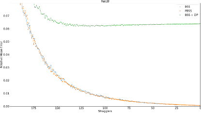
(a) ReLU computation comparison.

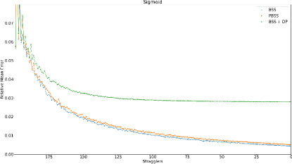
(b) Sigmoid computation comparison.

Stragglers	BSS	PBSS	BSS + DP
$100$	$0.006874037$	$0.006209476$	$0.062076736$
$50$	$0.002417026$	$0.002503581$	$0.063198365$
$0$	$0.000577592$	$0.000655003$	$0.063969884$

Stragglers	BSS	PBSS	BSS + DP
$100$	$0.010227901$	$0.011458554$	$0.028995183$
$50$	$0.006560695$	$0.007300909$	$0.028202122$
$0$	$0.004400018$	$0.005110319$	$0.027956606$

Figure 3: Numerical precision with activation functions ReLU and Sigmoid.

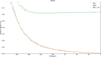
(a) Swish computation comparison.

Stragglers	BSS	PBSS	BSS + DP
$100$	$0.006389195$	$0.006893500$	$0.062273931$
$50$	$0.002165249$	$0.002500792$	$0.063192200$
$0$	$0.000596237$	$0.000675981$	$0.063865781$

Figure 4: Numerical precision with Swish activation function.

We have compared our proposal (PBSS) to the original BSS without privacy (BSS) and the original BSS adding a differential privacy scheme (BSS + DP). As it was previously mentioned, we have tested our proposal with three non-linear functions that are often used as activation functions in machine learning solutions: ReLU (Fig. 3a), Sigmoid (Fig. 3b) and Swish (Fig. 4a). We have used the normalized relative mean error as performance metric

$$\text{RME}=\frac{\|\frac{\tilde{Y}-Y}{Y}\|_{1}}{\text{len}(Y)},$$

where $Y$ is he exact result, $\tilde{Y}$ is its approximation, $\|\cdot\|_{1}$ is the entrywise $1$-norm of a matrix and $\text{len}()$ the total number of elements of a matrix (the division is done element by element).

Tables in Fig.3 show a summary of the the RME value when receiving different number of results from workers: $100$, $150$ and $200$, i.e. when the stragglers are $100$ nodes, $50$ nodes or $0$ nodes, respectively (note that the number of workers $N=200$ is defined in Table I).

As expected, since ReLU and Swish are similar functions, their behaviours are also similar. In both cases PBSS and BSS improve the numerical precision when the number of received results increases. However, the results obtained when applying BSS plus differential privacy are not so good. They do not improve when the number of results is higher than $50$, offering less privacy ($\sigma=30$) with no guarantees against colluding nodes. Therefore, the original BSS proposal (without privacy) offers slightly better results than our proposal (PBSS), being this a little cost to pay to include privacy in the computation. Precisely, the cost can be measured in terms of percentage of accuracy loss, being approximately $0.008\%$ for ReLU, $0.071\%$ for Sigmoid, and $0.008\%$ for Swish.

According to the results shown in Fig.3, the Sigmoid function seems to be harder to approximate than ReLU and Swish, since the precision obtained is lower than in the other two functions under BSS and PBSS. The precision performs better with Sigmoid than with ReLU or Swish using BSS + DP when the number of stragglers is less than $50$, although it does not outperform the results of our proposal.

We have also tested the precision results when using two typical aggregation functions in FL: Binary Step and the Median. As Fig. 5b shows, Median is harder to approximate than Binary Step (Fig. 5a). Since the errors for the aggregation functions are larger than in the previous case, more rounds would be needed for reaching model convergence that without including privacy.

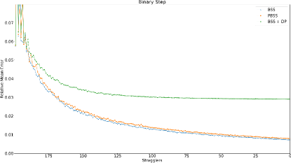
(a) Binary Step computation comparison.

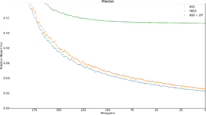
(b) Median computation comparison.

Stragglers	BSS	PBSS	BSS + DP
$100$	$0.012875861$	$0.013881484$	$0.030098946$
$50$	$0.009368434$	$0.010180803$	$0.029364728$
$0$	$0.007248344$	$0.007854828$	$0.029014532$

Stragglers	BSS	PBSS	BSS + DP
$100$	$0.044372558$	$0.049100067$	$0.116038774$
$50$	$0.031538214$	$0.034423612$	$0.113759435$
$0$	$0.022517222$	$0.025564940$	$0.112916117$

Figure 5: Precision results using different aggregation functions (Binary Step and Median). The Tables contain the relative errors.

To sum up, the errors we have obtained for the activation functions with PBSS are quite close to the ones obtained without privacy (BSS), working with large matrices ($K=1000$) and for a reasonable privacy level ($\imath_{L}=0.197$ bits). Thus, PBSS could be suitable for secure federated learning for classic machine learning models (linear/logistic regressions, neural networks, convolutional neural networks, etc.). Besides, the results obtained for the two aggregation methods, suggest that PBSS would fit in FL settings where the objective is to securely aggregate a model resilient to malicious adversaries. Additionally, PBSS should also be able to approximate complex aggregations that require comparisons (Binary step), e.g., in survival analysis with Cox regression. That said, as the errors for the aggregation functions are larger than in the previous case, it is likely that this will have an impact on the number of rounds it takes the model to converge.

VI-B Testing Matrix Multiplications

We also tested our proposal for matrix multiplications with two types of operations: common matrix multiplications (two inputs) and matrix multiplication in blocks (two inputs divided in blocks). We computed the numerical precision in presence of stragglers to compare our PBSS with the original BSS (without privacy) in order to evaluate the trade-off between privacy and accuracy. The matrices were randomly generated with entries drawn from a uniform distribution.

Fig. 6 shows the precision results when using the common matrix multiplication scheme proposed in Section V-B using conventional matrices (Fig. 6a) and sparse matrices (Fig. 6b. In both cases, PBSS offers almost identical results than the original scheme without privacy (BSS), so adding privacy does not have a high cost in performance. Anyway, it is worthy to mention that, as expected, the lower the number of stragglers the better the result achieved. But, differently to the results of the previous analysis (non-linear functions and aggregation functions in Section VI-A, BSS and PBSS perform worse in presence of stragglers, so they needs from more results to reduce the error. This behaviour is even more accentuated with sparse matrices.

Fig. 7 shows the precision results when applying the matrix multiplication scheme proposed in Section V-D2, where we detailed a way to divide the encoding of a matrix in vertical blocks, in such a way that the multiplication of matrices can be done in smaller blocks. For our analysis, we have used conventional matrices (Fig. 7a) and sparse matrices (Fig. 7b. As it can be seen in the tables of results and in the graphs, the numerical precision are identical as the matrix multiplications without dividing the matrices.

(a) Conventional Matrix multiplication.

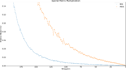
(b) Sparse Matrix Multiplication.

Stragglers	BSS	PBSS
$100$	$0.005357120$	$0.031209873$
$50$	$0.002866487$	$0.012143143$
$0$	$0.000995137$	$0.001074013$

Stragglers	BSS	PBSS
$100$	$0.007925727$	$0.051045426$
$50$	$0.003098950$	$0.017392449$
$0$	$0.000970545$	$0.001014285$

Figure 6: Common Matrix Multiplications computation. The Tables show the relative errors.

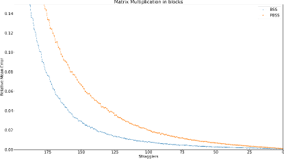
(a) Conventional Matrix multiplication divided in 2 vertical blocks.

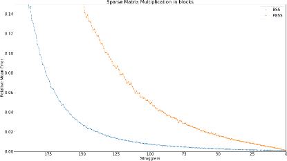
(b) Sparse Matrix multiplication divided in 2 vertical blocks.

Stragglers	BSS	PBSS
$100$	$0.008055111$	$0.019841101$
$50$	$0.002768221$	$0.006725834$
$0$	$0.000952427$	$0.000965228$

Stragglers	BSS	PBSS
$100$	$0.007520580$	$0.048800873$
$50$	$0.002710397$	$0.016400029$
$0$	$0.000928929$	$0.000949479$

Figure 7: Matrix Multiplications in blocks. The Tables show the relative errors for private (PBSS) and non-private (BSS) computations.

Similarly to what happens with the non-linear computations, the matrix products with PBSS show precision very close to BSS when the total number of collected results is high. However, matrix multiplication is specially sensitive to the presence of stragglers. This behaviour is even more notorious when computing sparse matrices. Thus, the privacy level in networks with a high proportion of straggler nodes must be carefully defined, but it is possible to provide strong privacy guarantees in homogeneous networks.

VII Conclusions

In this paper we proposed a solution, coined as Private BACC Secret Sharring (PBSS), able to assure privacy in FL and, simultaneously, able to deal with three important aspects that other previous approaches in literature have not solved: (i) working properly with non-linear functions, (ii) working properly with large matrix multiplications, (iii) reduce the high communications overheads due to the presence of semi-hones nodes and (iv) manage stragglers nodes without a high impact on precision. PBSS operate with the model parameters in the coded domain, ensuring output privacy in the nodes without any additional communication cost. Besides, our proposal could be leveraged in secure federated learning for the training of a wide range of machine learning algorithm, since it does not depend on the specific algorithms and it is able to operate with large matrix multiplication.

Since, as we have checked in our analysis, the errors for the aggregation functions are higher than those obtained for activation functions, we are currently working on providing suitable solutions for more complex model aggregation mechanisms in FL. Additionally, we expect to check the security guarantees in more realistic scenarios using well know attacks against our FL proposal.

References

- [1] M. Khan, F. G. Glavin, and M. Nickles, “Federated learning as a privacy solution - an overview,” Procedia Computer Science, vol. 217, pp. 316–325, 2023, 4th Int. Conf. on Industry 4.0 and Smart Manufacturing. [Online]. Available: https://www.sciencedirect.com/science/article/pii/S1877050922023055
- [2] L. Lyu, H. Yu, X. Ma, C. Chen, L. Sun, J. Zhao, Q. Yang, and S. Y. Philip, “Privacy and robustness in federated learning: Attacks and defenses,” IEEE Trans. on neural networks and learning systems, 2022.
- [3] L. Lyu, H. Yu, and Q. Yang, “Threats to federated learning: A survey,” arXiv preprint arXiv:2003.02133, 2020.
- [4] N. Carlini, S. Chien, M. Nasr, S. Song, A. Terzis, and F. Tramèr, “Membership inference attacks from first principles,” in 43rd IEEE Symp. on Security and Privacy, SP 2022, San Francisco, CA, USA, May 22-26, 2022. IEEE, 2022, pp. 1897–1914.
- [5] H. Hu, Z. Salcic, L. Sun, G. Dobbie, P. S. Yu, and X. Zhang, “Membership inference attacks on machine learning: A survey,” ACM Computing Surveys, vol. 54, no. 11s, pp. 1–37, 2022.
- [6] Z. Wang, M. Song, Z. Zhang, Y. Song, Q. Wang, and H. Qi, “Beyond inferring class representatives: User-level privacy leakage from federated learning,” in IEEE INFOCOM 2019-IEEE conference on computer communications. IEEE, 2019, pp. 2512–2520.
- [7] L. Melis, C. Song, E. De Cristofaro, and V. Shmatikov, “Exploiting unintended feature leakage in collaborative learning,” in 2019 IEEE Symp. on security and privacy (SP). IEEE, 2019, pp. 691–706.
- [8] J. Geiping, H. Bauermeister, H. Dröge, and M. Moeller, “Inverting gradients-how easy is it to break privacy in federated learning?” Adv. in neural information processing systems, vol. 33, pp. 16 937–16 947, 2020.
- [9] X. Yin, Y. Zhu, and J. Hu, “A comprehensive survey of privacy-preserving federated learning: A taxonomy, review, and future directions,” ACM Computing Surveys, vol. 54, no. 6, pp. 1–36, 2021.
- [10] C. Dwork, “Differential privacy,” in Int. Colloquium on Automata, Languages, and Programming. Berlin, Heidelberg: Springer, 2006, pp. 1–12.
- [11] M. Chase, H. Chen, J. Ding, S. Goldwasser, S. Gorbunov, J. Hoffstein, K. Lauter, S. Lokam, D. Moody, T. Morrison, A. Sahai, and V. Vaikuntanathan, “Security of homomorphic encryption,” HomomorphicEncryption.org, Redmond, WA, Tech. Rep., July 2017.
- [12] D. Evans, V. Kolesnikov, and M. Rosulek, “A pragmatic introduction to secure multi-party computation,” Foundations and Trends® in Privacy and Security, vol. 2, pp. 70–246, 2018.
- [13] P. K. et al., “Advances and open problems in federated learning,” Foundations and Trends in Machine Learning, vol. 14, no. 1–2, pp. 1–210, 2021. [Online]. Available: http://dx.doi.org/10.1561/2200000083
- [14] S. Sharma, S. Sharma, and A. Athaiya, “Activation functions in neural networks,” Towards Data Sci, vol. 6, no. 12, pp. 310–316, 2017.
- [15] B. George, S. Seals, and I. Aban, “Survival analysis and regression models,” Journal of Nuclear Cardiology, vol. 21, no. 4, pp. 686–694, 2014. [Online]. Available: https://www.sciencedirect.com/science/article/pii/S1071358123073154
- [16] S. Huda, J. Yearwood, H. F. Jelinek, M. M. Hassan, G. Fortino, and M. Buckland, “A hybrid feature selection with ensemble classification for imbalanced healthcare data: A case study for brain tumor diagnosis,” IEEE Access, vol. 4, pp. 9145–9154, 2016.
- [17] K. Pillutla, S. M. Kakade, and Z. Harchaoui, “Robust aggregation for federated learning,” IEEE Trans. on Signal Processing, vol. 70, pp. 1142–1154, 2022.
- [18] S. Li, E. Ngai, and T. Voigt, “Byzantine-robust aggregation in federated learning empowered industrial iot,” IEEE Trans. on Industrial Informatics, vol. 19, no. 2, pp. 1165–1175, 2023.
- [19] R. Yuster and U. Zwick, “Fast sparse matrix multiplication,” ACM Trans. Algorithms, vol. 1, no. 1, p. 2–13, jul 2005. [Online]. Available: https://doi.org/10.1145/1077464.1077466
- [20] S. Smith, N. Ravindran, N. D. Sidiropoulos, and G. Karypis, “Splatt: Efficient and parallel sparse tensor-matrix multiplication,” in 2015 IEEE Int. Parallel and Distributed Processing Symposium, 2015, pp. 61–70.
- [21] Z. Zhang, H. Wang, S. Han, and W. J. Dally, “Sparch: Efficient architecture for sparse matrix multiplication,” in 2020 IEEE Int. Symp. on High Performance Computer Architecture (HPCA), 2020, pp. 261–274.
- [22] S. Li and S. Avestimehr, “Coded computing: Mitigating fundamental bottlenecks in large-scale distributed computing and machine learning,” Foundations and Trends in Communications and Information Theory, vol. 17, no. 1, pp. 1–148, 2020. [Online]. Available: http://dx.doi.org/10.1561/0100000103
- [23] J. S. Ng, W. Y. B. Lim, N. C. Luong, Z. Xiong, A. Asheralieva, D. Niyato, C. Leung, and C. Miao, “A survey of coded distributed computing,” 2020.
- [24] A. Beimel, “Secret-sharing schemes: A survey,” in Int. Conf. on coding and cryptology. Springer, 2011, pp. 11–46.
- [25] A. K. Chattopadhyay, S. Saha, A. Nag, and S. Nandi, “Secret sharing: A comprehensive survey, taxonomy and applications,” Computer Science Review, vol. 51, p. 100608, 2024.
- [26] A. Shamir, “How to share a secret,” Commun. ACM, vol. 22, no. 11, pp. 612–613, nov 1979. [Online]. Available: https://doi.org/10.1145/359168.359176
- [27] T. Jahani-Nezhad and M. A. Maddah-Ali, “Berrut approximated coded computing: Straggler resistance beyond polynomial computing,” IEEE Trans. on Pattern Analysis and Machine Intelligence, vol. 45, no. 1, pp. 111–122, 2023.
- [28] S. Li, M. A. Maddah-Ali, Q. Yu, and A. S. Avestimehr, “A fundamental tradeoff between computation and communication in distributed computing,” IEEE Trans. on Inf. Theory, vol. 64, no. 1, pp. 109–128, 2017.
- [29] K. Lee, M. Lam, R. Pedarsani, D. Papailiopoulos, and K. Ramchandran, “Speeding up distributed machine learning using codes,” IEEE Trans. on Inf. Theory, vol. 64, no. 3, pp. 1514–1529, 2017.
- [30] S. Li, M. A. Maddah-Ali, and A. S. Avestimehr, “Coded mapreduce,” in 2015 53rd Annual Allerton Conf. on Communication, Control, and Computing (Allerton). IEEE, 2015, pp. 964–971.
- [31] S. Ulukus, S. Avestimehr, M. Gastpar, S. A. Jafar, R. Tandon, and C. Tian, “Private retrieval, computing, and learning: Recent progress and future challenges,” IEEE J. on Selected Areas in Communications, vol. 40, no. 3, pp. 729–748, 2022.
- [32] Q. Yu, S. Li, N. Raviv, S. M. M. Kalan, M. Soltanolkotabi, and S. A. Avestimehr, “Lagrange coded computing: Optimal design for resiliency, security, and privacy,” in Proc. of the 22nd Int. Conf. on Artificial Intelligence and Statistics, vol. 89. PMLR, 16–18 Apr 2019, pp. 1215–1225. [Online]. Available: https://proceedings.mlr.press/v89/yu19b.html
- [33] M. Soleymani, H. Mahdavifar, and A. S. Avestimehr, “Analog lagrange coded computing,” IEEE J. on Selected Areas in Information Theory, vol. 2, no. 1, pp. 283–295, 2021.
- [34] H. A. Nodehi and M. A. Maddah-Ali, “Secure coded multi-party computation for massive matrix operations,” in arXiv preprint arXiv:1908.04255, 2019.
- [35] M. Kim, H. Yang, and J. Lee, “Fully private and secure coded matrix multiplication with colluding workers,” ICT Express, vol. 9, no. 4, pp. 722–727, 2023. [Online]. Available: https://www.sciencedirect.com/science/article/pii/S2405959523000115
- [36] Q. Yu and A. S. Avestimehr, “Entangled polynomial codes for secure, private, and batch distributed matrix multiplication: Breaking the "cubic" barrier,” in 2020 IEEE Int. Symp. on Information Theory (ISIT), 2020, pp. 245–250.
- [37] T. Jahani-Nezhad and M. A. Maddah-Ali, “Codedsketch: A coding scheme for distributed computation of approximated matrix multiplication,” IEEE Trans. on Inf. Theory, vol. 67, no. 6, pp. 4185–4196, 2021.
- [38] J. Zhu, Q. Yan, X. Tang, and S. Li, “Symmetric private polynomial computation from lagrange encoding,” IEEE Trans. on Information Theory, vol. 68, no. 4, pp. 2704–2718, Apr. 2022.
- [39] N. Raviv and D. A. Karpuk, “Private polynomial computation from lagrange encoding,” in 2019 IEEE Int. Symp. on Information Theory (ISIT). IEEE, Jul. 2019.
- [40] I. Issa, A. B. Wagner, and S. Kamath, “An operational approach to information leakage,” IEEE Trans. on Information Theory, vol. 66, no. 3, pp. 1625–1657, 2020.
- [41] L. Schumacher, K. Pedersen, and P. Mogensen, “From antenna spacings to theoretical capacities - guidelines for simulating mimo systems,” in The 13th IEEE Int. Symp. on Personal, Indoor and Mobile Radio Communications, vol. 2, 2002, pp. 587–592 vol.2.
- [42] H. B. McMahan, E. Moore, D. Ramage, S. Hampson, and B. A. y Arcas, “Communication-efficient learning of deep networks from decentralized data,” in Int. Conf. on Artificial Intelligence and Statistics, 2016. [Online]. Available: https://api.semanticscholar.org/CorpusID:14955348
- [43] S. P. Karimireddy, S. Kale, M. Mohri, S. Reddi, S. Stich, and A. T. Suresh, “SCAFFOLD: Stochastic controlled averaging for federated learning,” in Proc. of the 37th Int. Conf. on Machine Learning, vol. 119. PMLR, 13–18 Jul 2020, pp. 5132–5143. [Online]. Available: https://proceedings.mlr.press/v119/karimireddy20a.html
- [44] Z. Zhu, J. Hong, and J. Zhou, “Data-free knowledge distillation for heterogeneous federated learning,” in Proc. of the 38th Int. Conf. on Machine Learning, ser. Proc. of Machine Learning Research, M. Meila and T. Zhang, Eds., vol. 139. PMLR, 18–24 Jul 2021, pp. 12 878–12 889. [Online]. Available: https://proceedings.mlr.press/v139/zhu21b.html