Optimization without retraction on the random generalized Stiefel manifold

Abstract

Optimization over the set of matrices that satisfy $X^{\top}BX=I_{p}$, referred to as the generalized Stiefel manifold, appears in many applications involving sampled covariance matrices such as canonical correlation analysis (CCA), independent component analysis (ICA), and the generalized eigenvalue problem (GEVP). Solving these problems is typically done by iterative methods, such as Riemannian approaches, which require a computationally expensive eigenvalue decomposition involving fully formed $B$. We propose a cheap stochastic iterative method that solves the optimization problem while having access only to a random estimate of the feasible set. Our method does not enforce the constraint in every iteration exactly, but instead it produces iterations that converge to a critical point on the generalized Stiefel manifold defined in expectation. The method has lower per-iteration cost, requires only matrix multiplications, and has the same convergence rates as its Riemannian counterparts involving the full matrix $B$. Experiments demonstrate its effectiveness in various machine learning applications involving generalized orthogonality constraints, including CCA, ICA, and GEVP.

1 Introduction

Many problems in machine learning and engineering, including the canonical correlation analysis (CCA) (Hotelling, 1936), independent component analysis (ICA) (Comon, 1994), linear discriminant analysis (McLachlan, 1992), and the generalized eigenvalue problem (GEVP) (Saad, 2011), can be formulated as the following optimization problem

$$\begin{gathered}\min_{X\in{\mathrm{St}_{B}(p,n)}}f(X):=\mathbb{E}[f_{\xi}(X)],\\ {\mathrm{St}_{B}(p,n)}:=\left\{X\in\mathbb{R}^{n\times p}|X^{\top}BX=I_{p}\right\}\text{ and }B=\mathbb{E}[B_{\zeta}],\end{gathered}$$ (1)

where the objective function $f$ is the expectation of $L$-smooth functions $f_{\xi}$, and $B\in\mathbb{R}^{n\times n}$ is a positive definite matrix defined as the expectation $B=\mathbb{E}_{\zeta}[B_{\zeta}]\succ 0$, and $\xi,\zeta$ are independent random variables. We assume that individual random matrices $B_{\zeta}$ do not need to be of full rank and are only positive semi-definite. The feasible set ${\mathrm{St}_{B}(p,n)}\subset\mathbb{R}^{n\times p}$ defines a smooth manifold referred to as the generalized Stiefel manifold.

In the deterministic case, when we have access to the matrix $B$, the optimization problem can be solved by Riemannian techniques (Absil et al., 2008; Boumal, 2023). Riemannian methods produce a sequence of iterates belonging to the set ${\mathrm{St}_{B}(p,n)}$, often by repeatedly applying a retraction that maps tangent vectors to points on the manifold. In the case of ${\mathrm{St}_{B}(p,n)}$ retractions require non-trivial linear algebra operations such as eigenvalue or Cholesky decomposition. On the other hand, optimization on ${\mathrm{St}_{B}(p,n)}$ also lends itself to infeasible optimization methods, such as the augmented Lagrangian method. Such methods are also typically employed in deterministic setting when the feasible set does not have a convenient projection, e.g. by the lack of a closed-form expression or because they require solving an expensive optimization problem themselves (Bertsekas, 1982). Infeasible approaches produce iterates that do not strictly remain in the feasible set but gradually converge to it by solving a sequence of unconstrained optimization problems. However, solving the optimization subproblems in each iteration might be computationally expensive and the methods are sensitive to the choice of hyper-parameters, both in theory and in practice.

In this paper, unlike in the aforementioned areas of study, we consider the setting (1) where the feasible set itself is stochastic, i.e. the matrix $B$ is unknown and is an expectation of random estimates $B_{\zeta}$, for which, neither Riemannian methods nor infeasible optimization techniques, are well-suited. In particular, we are interested in the case where we only have access to i.i.d. samples from $\xi$ and $\zeta$, and not to the full function $f$ and matrix $B$.

Figure 1: Illustration of the landing field on the random feasible set.

We design an iterative landing method requiring only a random estimates $B_{\zeta}$ that provably converges to a critical point of (1) while performing only matrix multiplications. The main principle of the method is depicted in the diagram in Figure 1 and is inspired by the recent line of work, but for the deterministic feasible set of the orthogonal set (Ablin & Peyré, 2022) and the Stiefel manifold (Gao et al., 2022b; Ablin et al., 2023; Schechtman et al., 2023). Instead of performing retractions after each iteration, the proposed algorithm only tracks an approximate distance to the constraint by following an unbiased estimator of the direction towards the manifold, while remaining within an initially prescribed $\varepsilon$-safe region, and finally “lands” on, i.e. converges to, the manifold.

The proposed stochastic landing iteration for solving (1) is a simple, cheap, and stochastic update rule

$$\begin{gathered}X^{k+1}=X^{k}-\eta_{k}\Lambda_{\xi^{k},\zeta^{k},\zeta^{\prime k}}(X^{k})\\ \text{with}\quad\Lambda_{\xi,\zeta,\zeta^{\prime}}(X)=\Psi_{\xi,\zeta,\zeta^{\prime}}(X)+\omega\nabla\mathcal{N}_{\zeta,\zeta^{\prime}}(X),\end{gathered}$$ (2)

in $\mathbb{R}^{n\times p}$ whose two components are

$$\begin{gathered}\Psi_{\xi,\zeta,\zeta^{\prime}}(X)=2\,{\mathrm{skew}}\left(\nabla f_{\xi}(X)X^{\top}B_{\zeta}\right)B_{\zeta^{\prime}}X\\ \nabla\mathcal{N}_{\zeta,\zeta^{\prime}}(X)=2B_{\zeta}X\left(X^{\top}B_{\zeta^{\prime}}X-I_{p}\right)\end{gathered},$$ (3)

where $\omega>0$, $\nabla\mathcal{N}_{\zeta,\zeta^{\prime}}(X)$ is an unbiased stochastic estimator of the gradient of $\mathcal{N}(X)=\frac{1}{2}\|X^{\top}BX-I_{p}\|_{\mathrm{F}}^{2}$, and ${\mathrm{skew}}(A)=(A-A^{\top})/2$. The above landing field formula (2) applies in the general case when both the function $f$ and the constraint matrix $B$ are stochastic; the deterministic case is recovered by substituting $\nabla f_{\xi}=\nabla f$ and $B_{\zeta}=B_{\zeta^{\prime}}=B$. Note that in many applications of interest, $B_{\zeta}=\sum_{i=1}^{r}x_{i}x_{i}^{\top}/r$ is a subsampled covariance matrix with batch-size $r$, that is of rank $r$ when $r\leq n$. Unlike retractions, the landing method benefits in this setting since the cost of multiplication by $B_{\zeta}$, which is the dominant cost of (2) becomes $\mathcal{O}(npr)$ instead of $\mathcal{O}(n^{2}p)$ where $r$ is the batch size. The landing method never requires to form the matrix $B$, thus having space complexity defined by only saving the iterates: $\mathcal{O}(np)$ instead of $\mathcal{O}(n^{2})$.

We prove that the landing iteration converges to an $e$-critical point, i.e. a point for which the Riemannian gradient is bounded by $e$ and $\|\mathcal{N}(X)\|\leq e$, with a fixed step size in the deterministic case (Theorem 2.7) and with decaying step size in the stochastic case (Theorem 2.8), with a rate that matches that of deterministic (Boumal et al., 2019) and stochastic Riemannian gradient descent (Bonnabel, 2013) on ${\mathrm{St}_{B}(p,n)}$. The advantages of the landing field in (2) are that i) its computation involves only parallelizable matrix multiplications, which is cheaper than the computations of the Riemannian gradient and retraction and ii) it handles gracefully the stochastic constraint, while Riemannian approaches need form the full estimate of $B$.

While the presented theory holds for a general smooth, possibly non-convex objective $f$, a particular problem that can be either phrased as (1) or framed as an optimization over the product manifold of two ${\mathrm{St}_{B}(p,n)}$ is CCA, which is a widely used technique for measuring similarity between datasets (Raghu et al., 2017). CCA aims to find the top-$p$ most correlated principal components $X,Y\in\mathbb{R}^{n\times p}$, for two zero-centered datasets $D_{1}=(d_{1}^{1},\dots,d_{1}^{N}),D_{2}=(d_{2}^{1},\dots,d_{2}^{N})\in\mathbb{R}^{n\times N}$ of $N$ iid samples from two different distributions and is formulated as

$$\begin{gathered}\min_{X,Y\in\mathbb{R}^{n\times p}}\mathbb{E}_{i}\left[-\operatorname{Tr}(X^{\top}d_{1}^{i}(d_{2}^{i})^{\top}Y)\right]\\ X^{\top}\mathbb{E}_{i}[d_{1}^{i}(d_{1}^{i})^{\top}]X=I_{p}\text{ and }Y^{\top}\mathbb{E}_{i}[d_{2}^{i}(d_{2}^{i})^{\top}]Y=I_{p},\end{gathered}$$ (4)

where the expectations are w.r.t. the uniform distribution over $\{1,\ldots,N\}$. Here, the constraint matrices $B_{\zeta}$ correspond to individual or mini-batch sample covariances, and the constraints are that the two matrices $X,Y\in\mathbb{R}^{n\times p}$ are in the generalized Stiefel manifold.

The rest of the introduction gives a brief overview on the current optimization techniques for solving (1) and its forthcoming generalization (5) when the feasible set is deterministic, since we are not aware of existing techniques for (1) with stochastic feasible set. The rest of the paper is organized as follows.

• In Section 2 we give a form to a generalized landing algorithm for solving a smooth optimization problem $\min_{x\in\mathcal{M}}f(x)$ on a smooth manifold $\mathcal{M}$ defined below in  (5), which under suitable assumptions, converges to a critical point with the same sublinear rate $\mathcal{O}(1/K)$, as its Riemannian counterpart (Boumal et al., 2019), see Theorem 2.7, where $K$ is the iteration number. Unlike previous works (Schechtman et al., 2023; Ablin et al., 2023), our analysis is based on a smooth merit function allowing us to obtain a convergence result for the stochastic variant of the algorithm, when having an unbiased estimator for the landing field, see Theorem 2.8.

• In Section 3 we build on the general theory developed in the previous section and prove that the update rule for the generalized Stiefel manifold in (2) converges to a critical point of (1), both in the deterministic case with the rate $\mathcal{O}(1/K)$, and in expectation with the rate $\mathcal{O}(1/\sqrt{K})$ in the case when both the gradient of the objective function and the feasible set are stochastic estimates.

• In Section 4 we numerically demonstrate the efficiency of the proposed method on a deterministic example of solving a generalized eigenvalue problem, stochastic CCA and ICA.

Notation. We denote vectors by lower case letters $x,y,z,\ldots$, matrices with uppercase letters $X,Y,Z,\ldots$, and $I_{n}$ denotes the $n\times n$ identity matrix. Let $\mathrm{D}f(x)[v]=\lim_{t\rightarrow 0}(f(x+tv)-f(x))/t$ denote the derivative of $f$ at $x$ along $v$. The $\|\cdot\|$ denotes the $\ell_{2}$-norm or the Frobenius norm for matrices, whereas $\|\cdot\|_{2}$ denotes the operator norm induced by $\ell_{2}$-norm.

1.1 Prior work related to the optimization on the generalized Stiefel manifold

Riemannian optimization.

A widely used approach to solving the optimization problems constrained to manifolds as in (5) are the techniques from Riemannian optimization. These methods are based on the observation that smooth sets can be locally approximated by a linear subspace, which allows to extend classical Euclidean optimization methods, such as gradient descent and the stochastic gradient descent to the Riemannian setting. For example, Riemannian gradient descent iterates $x^{k+1}=\mathrm{Retr}_{\mathcal{M}}(x^{k},-\eta_{k}{\mathrm{grad}}f(x^{k}))$, where $\eta_{k}>0$ is the stepsize at iteration $k$, ${\mathrm{grad}}f(x^{k})$ is the Riemannian gradient that is computed as a projection of $\nabla f(x^{k})$ on the tangent space of $\mathcal{M}$ at $x^{k}$, and $\mathrm{Retr}$ is the retraction operation, which projects the updated iterate along the direction $-\eta_{k}{\mathrm{grad}}f(x^{k})$ on the manifold and is accurate up to the first-order, i.e., $\mathrm{Retr}_{\mathcal{M}}(x,d)=x+d+o(\|d\|)$. Retractions allow the implementation of Riemannian counterparts to classical Euclidean methods on the generalized Stiefel manifold, such as Riemannian (stochastic) gradient descent (Bonnabel, 2013; Zhang & Sra, 2016), trust-region methods (Absil et al., 2007), and accelerated methods (Ahn & Sra, 2020); for an overview, see (Absil et al., 2008; Boumal, 2023).

	Matrix factorizations	Complexity
Polar	matrix inverse square root	$\mathcal{O}(n^{2}p)$
SVD-based	SVD	$\mathcal{O}(n^{2}p)$
Cholesky-QR	Cholesky, matrix inverse	$\mathcal{O}(n^{2}p)$
$\Lambda(X)$ formula in (2)	None	$\min\{\mathcal{O}(n^{2}p),\mathcal{O}(npr)\}$

Table 1: Cost comparison of retractions and the landing formula on the generalized Stiefel manifold. The matrices are of size $n\times p$ with $p\leq n$, and $r$ is the rank of the stochastic matrices $B_{\zeta}$. Matrix factorizations are hard to parallelize. The retractions do not allow for reduced complexities when $B_{\zeta}$ is low-rank and are not suited for stochastic $B_{\zeta}$.

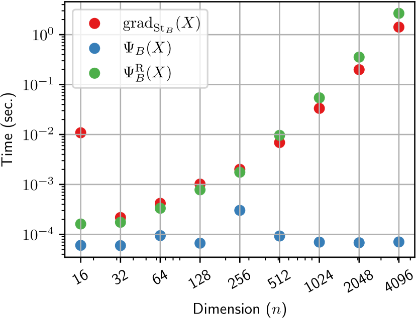
(a) Descent directions.

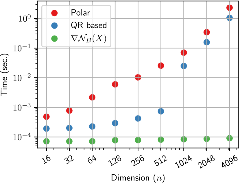
(b) Retractions.

Figure 7: Comparison of per-iteration computational time for different problem sizes of the descent directions of algorithms in Fig. 3 and the cost of retractions compared to $\nabla\mathcal{N}(X)$, both in the deterministic setting when $n=p=r$, for which the matrix multiplication in $\Psi_{B}(X)$ and $\nabla_{\mathcal{N}}(X)$ are at the disadvantage. Computation time of randomly generated $B,X\in\mathbb{R}^{n\times n}$ averaged over $100$ runs with CUDA implementation using cupy.

There are several ways to compute a retraction to the generalized Stiefel manifold, which we summarize in Table 1 and we give a more detailed explanation in Appendix A. Overall, we see that the landing field (2) is much cheaper to compute than all these retractions in two cases: i) when $n\simeq p$, then the bottleneck in the retractions becomes the matrix factorization, which, although they are of the same complexity as matrix multiplications, are much more expensive and hard to parallelize, ii) when $n$ gets extremely large, the cost of all retractions grows quadratically with $n$, while the use of mini-batches of size $r$ allows computing the landing field in linear time. We demonstrate numerically the practical cost of computing retractions in Fig 7(b) in the appendices.

Infeasible optimization methods.

A popular approach for solving constrained optimization is to employ the squared $\ell_{2}$-penalty method by adding the $\omega\mathcal{N}(X)$ regularizer to the objective. However, unlike the landing method, the iterates of the squared penalty method do not converge to the constraint exactly for any fixed choice of $\omega$ and converge only when $\omega$ are increasing in iterations (Nocedal & Wright, 2006). In contrast, the landing method provably converges to the constraint for any fixed $\omega>0$, which is enabled by the gradient component having a Riemannian interpretation and being orthogonal to the normalizing component.

Infeasible methods, such as the augmented Lagrangian methods, with an augmented Lagrangian function $\mathcal{L}(x,\lambda)$, such as the one introduced later in (9), by updating the solution vector $x$ and the vector of Lagrange multipliers $\lambda$ respectively (Bertsekas, 1982). This is typically done by solving a sequence of optimization problems of $\mathcal{L}(\cdot,\lambda_{k})$ followed by a first-order update of the multipliers $\lambda_{k+1}=\lambda_{k}-\beta h(x_{k})$ depending on the penalty parameter $\beta$. The iterates are gradually pushed towards the constraint by increasing the penalty parameter $\beta$. However, each optimization subproblem may be expensive, and the methods are sensitive to the choice of the penalty parameter $\beta$.

Recently, a number of works explored the possibility of infeasible methods for optimization on Riemannian manifolds, when the feasible set is deterministic, in order to eliminate the cost of retractions, which can be limiting in some situations, e.g. when the evaluation of stochastic gradients is cheap. The works of (Gao et al., 2019a, 2022a) proposed a modified augmented Lagrangian method which allows for fast computation and better better bounds on the penalty parameter $\beta$. (Ablin & Peyré, 2022) designed a simple iterative method called landing, consisting of two orthogonal components, to be used on the orthogonal group, which was later expanded to the Stiefel manifold (Gao et al., 2022b; Ablin et al., 2023). (Schechtman et al., 2023) expanded the landing approach to be used on a general smooth constraint using a non-smooth merit function. More recently, (Goyens et al., 2023) analysed the classical Fletcher’s augmented Lagrangian for solving smoothly constrained problems through the Riemannian perspective and proposed an algorithm that provably finds second-order critical points of the minimization problem.

1.2 Methods for the GEVP and CCA

Stochastic Matrix factorizations Total operation count complexity for $e$-criticality Memory AppGrad^* (Ma et al., 2015) - SVD $\mathcal{O}((n^{2}p\kappa_{B}+p^{2}n)\delta^{-1}\log(1/e)+Nn^{2})$ $n^{2}$ CCALin (Ge et al., 2016) - linear solver $\mathcal{O}((n^{2}p\sqrt{\kappa_{B}}+p^{2}n)\delta^{-1}\log(1/e)+Nn^{2})$ $n^{2}$ rgCCALin (Xu & Li, 2020) - linear solver $\mathcal{O}((n^{2}p\sqrt{\kappa_{B}}+p^{2}n)\delta^{\prime-2}\log(1/e)+Nn^{2})$ $n^{2}$ LazyCCA (Allen-Zhu & Li, 2017) - linear solver $\mathcal{O}((n^{2}p\sqrt{\kappa_{B}}+p^{2}n)\delta^{-1/2}\log(1/e)+Nn^{2})$ $n^{2}$ MSG (Arora et al., 2017) ✓ inverse square root $\mathcal{O}(n^{3}(p(\sigma^{\prime})^{2}+p^{2}\kappa_{B}^{2})/e^{2})$ $n^{2}$ $\Lambda(X)$ formula^$\dagger$ in (2) ✓ None $\mathcal{O}(\kappa_{B}^{5}\sigma^{2}np/e^{2})$ $np$

Table 2: Overview of CCA and GEVP solvers for finding top-$p$ vectors simultaneously that achieve $e$-critical point, i.e. $\|{\mathrm{grad}}f(X^{k})\|\leq e$. We assume that the number of samples is much greater than the dimension, i.e. $N\gg n$ and denote $\kappa_{B}=\beta_{1}/\beta_{n}$ to be the condition number of $B$. Deterministic methods depend on the gap $\delta=\beta_{p}-\beta_{p+1}$, while stochastic methods are independent of the $\delta$ and depend on the variance, where $\sigma^{\prime}$ is the variance of the data $x$, whereas $\sigma$ is the variance of the covariance estimate $xx^{\top}$. The first three methods achieve linear rate $\mathcal{O}(\log(1/e))$, while the last two methods have sublinear rate $\mathcal{O}(1/e^{2})$. “Stochastic” marks methods with convergence analysis for the stochastic case. Deterministic methods require forming the matrix $B$ at the start with additional cost $\mathcal{O}(Nn^{2})$. ^*marks local convergence result to the minimum and ^$\dagger$marks convergence to a critical point.

Deterministic methods.

A lot of effort has been spent in recent years on finding fast and memory-efficient solvers for CCA and the GEVP, that seeks to find a solution to $Ax=\lambda Bx$, both of which can be framed as (1). The majority of the existing methods specialized for CCA and GEVP that compute the top-$p$ vector solution aim to circumvent the need to compute $B^{-\frac{1}{2}}$ or $B^{-1}$, e.g. by using an approximate solver to compute the action of multiplying with $B^{-1}$. The classic Lanczos algorithm for computation of eigenvalues can be adapted to the GEVP by noting that we can look for standard eigenvectors of $B^{-1}A$, see (Saad, 2011, Algorithm 9.1). (Ma et al., 2015) proposes AppGrad which performs a projected gradient descent with $\ell_{2}$-regularization and proves its convergence when initialized sufficiently close to the minimum. The work of (Ge et al., 2016) proposes GenELinK algorithm based on the block power method, using inexact linear solvers, that has provable convergence with a rate depending on $1/\delta$, where $\delta=\beta_{p}-\beta_{p+1}$ is the eigenvalue gap. (Allen-Zhu & Li, 2017) improves upon this in terms of the eigenvalue gap and proposes the doubly accelerated method LazyCCA, which is based on the shift-and-invert strategy with iteration complexity that depends on $1/\sqrt{\delta}$. (Xu & Li, 2020) present a first-order Riemannian algorithm that computes gradients using fast linear solvers to approximate the action of $B^{-1}$ and performs polar retraction. (Meng et al., 2021) presents a Riemannian optimization technique that finds top-$p$ vectors using online estimates of the covariance matrices with $\mathcal{O}(n^{2}p)$ per-iteration computational cost and convergence rate of $\mathcal{O}(1/K)$.

Stochastic methods.

While the stochastic CCA problem is of high practical interest, fewer works consider it. Although several of the aforementioned deterministic solvers can be implemented for streaming data using sampled information (Ma et al., 2015; Wang et al., 2016; Meng et al., 2021), they do not analyse stochastic convergence. The main challenge comes from designing an unbiased estimator for the whitening part of the method that ensures the constraint $X^{\top}BX=I$ in expectation. (Arora et al., 2017) propose a stochastic approximation algorithm, MSG, that keeps a running weighted average of covariance matrices used for projection, requiring computing $B^{-1/2}$ at each iteration. Additionally, the work of (Gao et al., 2019b) proves stochastic convergence of an algorithm based on the shift-and-invert scheme and SVRG to solve linear subproblems, but only for the top-$1$ setting.

Comparison with the landing.

Constrained optimization methods such as the augmented Lagrangian methods and Riemannian optimization techniques can be applied on stochastic problems only when the gradient of the objective function is random, however, not on problems when the feasible set is stochastic. The landing method has provable global convergence guarantees with the same asymptotic rate as its Riemannian counterpart, while also allowing for stochasticity in the constraint. Our work is conceptually related to the recently developed infeasible methods (Ablin & Peyré, 2022; Ablin et al., 2023; Schechtman et al., 2023), with the key difference of constructing a smooth merit function for a general constraint $h(x)$, which is necessary for the convergence analysis of stochastic iterative updates that can have error in the normal space of $\mathcal{M}$. In Table 2 we show the overview of relevant GEVP/CCA methods by comparing their asymptotic operations cost required to converge to an $e$-critical point. The operation count takes into account both the number of iterations and the per-iteration cost, which is bounded asymptotically for the landing in Proposition 3.4. Despite the landing iteration (2) being designed for a general non-convex smooth problem (1) and not being tailored specifically to GEVP/CCA, we achieve theoretically interesting rate, which outperforms the other methods for well-conditioned matrices, when $\kappa$ is small, and when the variance of samples is small. Additionally, we provide an improved space complexity $\mathcal{O}(np)$ by not having to form the full matrix $B$ and only to save the iterates.

2 Generalized landing with stochastic constraints

This section is devoted to analyzing the landing method in the general case where the constraint is given by the zero set of a smooth function. We will later use these results in Section 3 devoted to extending and analyzing the landing method (2) on ${\mathrm{St}_{B}(p,n)}$. The theory presented here improves on that of Schechtman et al. (2023) in two important directions. First, we generalize the notion of relative descent direction, which allows us to consider a richer class than that of geometry-aware orthogonal directions (Schechtman et al., 2023, Eq.18). Second, we do not require any structure on the noise term $\tilde{E}$ defined later in (10), for the stochastic case, while A2(iii) in (Schechtman et al., 2023) requires the noise to be in the tangent space. This enhancement is due to the smoothness of our merit function $\mathcal{L}$, while Schechtman et al. (2023) consider a non-smooth merit function. Importantly, for the case of ${\mathrm{St}_{B}(p,n)}$ with the formula given in (2), there is indeed noise in the normal space, rendering Schechtman et al. (2023)’s theory inapplicable, while we show in the next section that Theorem 2.8 applies in that case.

Given a continuously differentiable function $f:\mathbb{R}^{d}\rightarrow\mathbb{R}$, we address the optimization problem:

$$\min_{x\in\mathbb{R}^{d}}f(x)\qquad\mathrm{s.\,t.}\quad x\in\mathcal{M}=\left\{x\in\mathbb{R}^{d}\,:\,h(x)=0\right\},$$ (5)

where $h:\mathbb{R}^{d}\rightarrow\mathbb{R}^{q}$ is continuously differentiable, non-convex, $q\in\mathbb{N}$ represents the number of constraints, and $\mathcal{M}$ defines a smooth manifold set. We will consider algorithms that stay within an initially prescribed $\varepsilon$-proximity region

$$\mathcal{M}^{\varepsilon}=\left\{x\in\mathbb{R}^{d}\,:\,\|h(x)\|\leq\varepsilon\right\}.$$ (6)

The first assumption we make is a blanket assumption from $f$ having a smooth derivative. The second one requires that the differential $\mathrm{D}h(x)^{*}$ inside the $\varepsilon$-safe region has bounded singular values.

Assumption 2.1 (Smoothness of the objective).

The objective function $f:\mathbb{R}^{d}\rightarrow\mathbb{R}$ is continuously differentiable and its gradient is $L_{f}$-Lipschitz.

Assumption 2.2 (Smoothness of the constraint).

Let $\mathrm{D}h(x)^{*}:\mathbb{R}^{q}\rightarrow\mathbb{R}^{d}$ be the adjoint of the differential of the constraint function $h$. The adjoint of the differential has bounded singular values for $x$ in the safe $\varepsilon$-region, i.e., $\forall x\in\mathcal{M}^{\varepsilon}:\quad\bar{C}_{h}\leq\sigma\left(\mathrm{D}h(x)^{*}\right)\leq C_{h}.$ Additionally, the gradient $\nabla\mathcal{N}(x)$ of the penalty term $\mathcal{N}(x)=\frac{1}{2}\|h(x)\|^{2}$ is Lipschitz continuous with constant $L_{\mathcal{N}}$ over $\mathcal{M}^{\varepsilon}$.

Assumption 2.1 is standard in optimization. Assumption 2.2 is necessary for the analysis of smooth constrained optimization (Goyens et al., 2023) and holds, e.g., when $\mathcal{M}^{\varepsilon}$ is a compact set, $\mathrm{D}h(x)^{*}$ is smooth, and $\mathrm{D}h(x)$ has full rank for all $x\in\mathcal{M}^{\varepsilon}$. Next, we define a relative gradient descent direction $\Psi(x)$, which is an extension of the Riemannian gradient outside of the manifold.

Definition 2.1 (Relative descent direction).

A relative descent direction $\Psi(x):\mathbb{R}^{d}\rightarrow\mathbb{R}^{d}$, with a parameter $\rho>0$ that may depend on $\varepsilon$ satisfies:

1. $\forall x\in\mathcal{M}^{\varepsilon},\quad\forall v\in\mathrm{span}(\mathrm{D}h(x)^{*}):\left\langle\Psi(x),\,v\right\rangle=0$;

2. $\forall x\in\mathcal{M}^{\varepsilon},\quad\left\langle\Psi(x),\,\nabla f(x)\right\rangle\geq\rho\|\Psi(x)\|^{2}$;

3. $\forall x\in\mathcal{M},\quad\left\langle\Psi(x),\,\nabla f(x)\right\rangle=0$ if and only if $x$ is a critical point of $f$ on $\mathcal{M}$.

In short, the relative descent direction must be orthogonal to the normal space $\mathrm{span}(\mathrm{D}h(x)^{*})$ while remaining positively aligned with the Euclidean gradient $\nabla f(x)$. While there may be many examples of relative descent directions, a particular example is the Riemannian gradient of $f$ with respect to the sheet manifold $h(x)=c$ when $\|c\|\leq\varepsilon$. Note, the above definition is not scale invariant to $\rho$, i.e. taking $c\Psi(x)$ for $c>0$ will result in $c\rho$, and this is in line with the forthcoming convergence guarantees deriving upper bound on $\|\Psi(x)\|$.

Proposition 2.2 (Riemannian gradient is a relative descent direction).

The Riemannian gradient of $f$ with respect to the sheet manifold $h(x)=c$, defined as

$${\mathrm{grad}}f(x)=\nabla f(x)-\mathrm{D}h(x)^{*}\left(\mathrm{D}h(x)^{*}\right)^{\dagger}\nabla f(x),$$ (7)

where $c\in\mathbb{R}^{p}$ is an error term such that $\|c\|\leq\varepsilon$, $\mathrm{D}h(x)$ denotes a differential, and $\mathrm{D}h(x)^{*}\left(\mathrm{D}h(x)^{*}\right)^{\dagger}$ acts as a projection on the normal space of $h(x)=c$ at $x$, is a relative descent direction on $\mathcal{M}^{\varepsilon}$ with $\rho=1$.

The proof can be found in the appendices in Subsection C.1. Such extension of the Riemannian gradient to the whole space was already considered by Gao et al. (2022b) in the particular case of the Stiefel manifold and by Schechtman et al. (2023). We now define the general form of the deterministic landing iteration as

$$x^{k+1}=x^{k}-\eta_{k}\Lambda(x^{k})\,\text{with}\,\Lambda(x)=\Psi(x)+\omega\nabla\mathcal{N}(x),$$ (8)

where $\Psi(x)$ is a relative descent direction described in Def. 2.1, $\nabla\mathcal{N}(x)$ is the gradient of the penalty $\mathcal{N}(x)=\frac{1}{2}\|h(x)\|^{2}$ weighted by the parameter $\omega>0$, $\nabla\mathcal{N}(x)=\mathrm{D}h(x)^{*}h(x)$, and $\|\cdot\|$ is the $\ell_{2}$-norm. The stochastic iterations, where noise is added at each iteration, will be introduced later in (10). Condition (i) in Def. 2.1 guarantees that $\left\langle\nabla\mathcal{N}(x),\,\Psi(x)\right\rangle=0$, so that the two terms in $\Lambda$ are orthogonal.

Note that we can use any relative descent directions as $\Psi$ depending on the specific problem. The Riemannian gradient in (7) is just one special case, which has some shortcomings. Firstly, it requires a potentially expensive projection $\mathrm{D}h(x)^{*}\left(\mathrm{D}h(x)^{*}\right)^{\dagger}$. Secondly, if the constraint involves a random noise on $h$, formula (7) it does not give an unbiased formula in expectation. An important contribution of the present work is the derivation of a computationally convenient form for the relative descent direction in the specific case of the generalized Stiefel manifold in Section 3.

We now turn to the analysis of the convergence of this method. The main object allowing for the convergence analysis is Fletcher’s augmented Lagrangian

$$\mathcal{L}(x)=f(x)-\left\langle h(x),\,\lambda(x)\right\rangle+\beta\|h(x)\|^{2},$$ (9)

with the Lagrange multiplier $\lambda(x)\in\mathbb{R}^{p}$ defined as $\lambda(x)=(\mathrm{D}h(x)^{*})^{\dagger}[\nabla f(x)].$ The differential of $\lambda(x)$ must be smooth, which is met when $h$ is continuously differentiable and $\mathcal{M}^{\varepsilon}$ is a compact set.

Assumption 2.3 (Multipliers of Fletcher’s augmented Lagrangian).

The norm of the differential of the multipliers of Fletcher’s augmented Lagrangian is bounded: $\sup_{x\in\mathcal{M}^{\varepsilon}}\|\mathrm{D}\lambda(x)\|\leq C_{\lambda}.$

Proposition 2.3 (Lipschitz constant of Fletcher’s augmented Lagrangian).

Fletcher’s augmented Lagrangian $\mathcal{L}$ in (9) is $L_{\mathcal{L}}$-smooth on $\mathcal{M}^{\varepsilon}$, with $L_{\mathcal{L}}=L_{f+\lambda}+L_{\mathcal{N}}$, where $L_{f+\lambda}$ is the smoothness constant of $f(x)+\left\langle\lambda(x),\,h(x)\right\rangle$ and $L_{\mathcal{N}}$ is that of $\mathcal{N}(x)$.

The following two lemmas show that there exists a positive step-size $\eta$ that guarantees that the next landing iteration stays within $\mathcal{M}^{\varepsilon}$ provided that the current iterate is inside $\mathcal{M}^{\varepsilon}$.

Lemma 2.4 (Upper bound on the safe step size).

Let $x\in\mathcal{M}^{\varepsilon}$ and consider the iterative update $\tilde{x}=x-\eta\Lambda(x)$, where $\eta>0$ is a step size and $\Lambda(x)$ is the landing field in (8). If the step size satisfies $\eta\leq\eta(x)$ with

$$\eta(x ):=\frac{1}{{L_{\mathcal{N}}\|\Lambda(x)\|^{2}}}\Big{(}\omega\|\nabla\mathcal{N}(x)\|^{2}+$$

$$\sqrt{\omega^{2}\|\nabla\mathcal{N}(x)\|^{4}+L_{\mathcal{N}}\|\Lambda(x)\|^{2}(\varepsilon^{2}-\|h(x)\|^{2})}\Big{)}$$

where $L_{\mathcal{N}}$ is from Assumption 2.2, then the line segment from the current to the next iterate remains in the safe region.

The proof can be found in the appendices in Subsection C.2. Next, we require that the norm of the relative descent direction must remain bounded in the safe region.

Assumption 2.4 (Bounded relative descent direction).

We require that $\sup_{x\in\mathcal{M}^{\varepsilon}}\|\Psi(x)\|\leq C_{\Psi}.$

This holds, for instance, if $\nabla f$ is bounded in $\mathcal{M}^{\varepsilon}$, using Def. 2.1 (ii) and Cauchy-Schwarz inequality. Under this assumption, we can lower bound the safe step in Lemma 2.4 for all $x\in\mathcal{M}^{\varepsilon}$, implying that there is always a positive step size that keeps the next iterate in the safe region.

Lemma 2.5 (Non-disappearing safe step size).

The upper bound on the safe step size in Lemma 2.4 is lower bounded as $\eta(x)\geq\min\left\{\frac{\varepsilon}{\sqrt{2L_{\mathcal{N}}}C_{\Psi}},\,\frac{\omega\bar{C}_{h}^{2}\varepsilon^{2}}{L_{\mathcal{N}}(C_{\Psi}^{2}+\omega^{2}C_{h}\varepsilon^{2})}\right\}\enspace\text{for all }x\in\mathcal{M}^{\varepsilon}$ where $C_{h},\bar{C}_{h},C_{\Psi}>0$ are constants from Assumption 2.2 and 2.4.

The proof can be found in Subsection C.3.

Lemma 2.6.

Let $\mathcal{L}(x)$ be Fletcher’s augmented Lagrangian in (9) with $\beta{\geq}(\frac{\rho}{4C_{h}^{2}}+\frac{C_{\lambda}}{2C_{h}}+\frac{C_{\lambda}^{2}}{C_{h}^{2}})/\omega$, where $\rho$ is defined in Def. 2.1. We have that $\left\langle\nabla\mathcal{L}(x),\,\Lambda(x)\right\rangle\geq\frac{\rho}{2}\left(\|\Psi(x)\|^{2}+\|h(x)\|^{2}\right).$

The proof can be found in the appendices in Subsection C.4. This critical lemma shows that $\mathcal{L}$ is a valid merit function for the landing iterations and allows the study of convergence of the method with ease. The following statement combines Lemma 2.6 with the bound on the safe step size in Lemma 2.5 to prove sublinear convergence to a critical point on the manifold.

Theorem 2.7 (Deterministic landing).

The landing iteration in (8) starting from $x_{0}\in\mathcal{M}^{\varepsilon}$ satisfies

$$\frac{1}{K}\sum_{k=0}^{K}\|\Psi(x^{k})\|^{2} \leq 4\frac{\mathcal{L}(x^{0})-\mathcal{L}^{*}}{\eta\rho K},$$

$$\frac{1}{K}\sum_{k=0}^{K}\|h(x_{k})\|^{2} \leq 4\frac{\mathcal{L}(x^{0})-\mathcal{L}^{*}}{\eta\rho\omega^{2}K}.$$

for $\eta\leq\min\left\{\frac{\rho}{2L_{\mathcal{L}}},\frac{\rho}{2L_{\mathcal{L}}C_{h}^{2}},\frac{\varepsilon}{\sqrt{2L_{\mathcal{N}}}C_{\Psi}},\,\frac{\omega\bar{C}_{h}^{2}\varepsilon^{2}}{L_{\mathcal{N}}(C_{\Psi}^{2}+\omega^{2}C_{h}\varepsilon^{2})}\right\}$ and $\mathcal{L}^{*}=\min_{x\in\mathcal{M}^{\varepsilon}}\mathcal{L}(x)$.

The proof is given in Subsection C.5 and implies the iterates $x^{k}$ converge to a critical point with the sublinear rate $\mathcal{O}(1/K)$.

Due to the smoothness of Fletcher’s augmented Lagrangian in the $\mathcal{M}^{\varepsilon}$ region, we can extend the convergence result to the stochastic setting, where the iterates are

$$x^{k+1}=x^{k}-\eta_{k}\left[\Lambda(x^{k})+\tilde{E}(x^{k},\Xi^{k})\right],$$ (10)

where the $\Xi^{k}$ are random i.i.d. variables and $\tilde{E}(x^{k},\Xi^{k})$ is the random error term at iteration $x^{k}$, and $\Lambda(x^{k})$ is the landing field in (8). We require the landing update in (10) to be an unbiased estimator with bounded variance.

Assumption 2.5 (Zero-centered and bounded variance).

There exists $\gamma>0$ such that for all $x\in\mathcal{M}^{\varepsilon}$, we have $\mathbb{E}_{\Xi}[\tilde{E}(x,\Xi)]=0$ and $\mathbb{E}_{\Xi}[\|\tilde{E}(x,\Xi)\|^{2}]\leq\gamma^{2}$.

We obtain the following result with decaying step sizes.

Theorem 2.8 (Stochastic landing).

The stochastic landing iteration in (10) with a diminishing step size $\eta_{k}=\eta_{0}\times(1+k)^{-1/2}$, whose updates are unbiased estimators with bounded variance as in Assumption 2.5 and assuming the line segments between the iterates remain within $\mathcal{M}^{\varepsilon}$ with probability one, produces iterates for which

$$\inf_{k\leq K}\mathbb{E}\left[\|\Psi(x_{k})\|^{2}\right]\leq\frac{4}{\rho\eta_{0}\sqrt{K}}\left(\mathcal{L}(x^{0})-\mathcal{L}^{*}+c\gamma^{2}\log(K)\right)$$

$$\inf_{k\leq K}\mathbb{E}\left[\|h(x)\|^{2}\right]\leq\frac{4}{\rho\omega^{2}\eta_{0}\sqrt{K}}\left(\mathcal{L}(x^{0})-\mathcal{L}^{*}+c\gamma^{2}\log(K)\right),$$

where $c=\frac{\eta_{0}L_{\mathcal{L}}}{2}$ for $\eta_{0}\leq\frac{\rho}{2L_{\mathcal{L}}}\min\left\{1,C_{h}^{-2}\right\}$ and $\mathcal{L}^{*}=\min_{x\in\mathcal{M}^{\varepsilon}}\mathcal{L}(x)$.

The theorem is proved in subsection C.6. Unlike in the deterministic case in Lemma 2.4, without further assumption on the distribution of $\Xi^{k}$, it cannot be ensured that the iterates $x^{k}$, or the line segments connecting them, are within $\mathcal{M}^{\varepsilon}$ with probability one. Under the assumption that the line segments between the iterates remain in the safe region, we recover the same convergence rate as Riemannian SGD in the non-convex setting for a deterministic constraint (Bonnabel, 2013), but in our case, we require only an online estimate of the random manifold constraint.

3 Landing on the generalized Stiefel manifold

This section builds on the results of the previous Section 2 and proves that the simple landing update rule $X^{k+1}=X^{k}-\eta_{k}\Lambda(X^{k})$, as defined as in (2), converges to the critical points of (1). The generalized Stiefel manifold ${\mathrm{St}_{B}(p,n)}$ is defined by the constraint function $h(X)=X^{\top}BX-I_{p}$, and we have $\nabla\mathcal{N}(X)=2BX(X^{T}BX-I_{p})$. We now derive the quantities required for Assumption 2.2.

Proposition 3.1 (Smoothness constants for the generalized Stiefel manifold).

Smoothness constants in Assumption 2.2 for the generalized Stiefel manifold are

$$C_{h}=2\sqrt{(1+\varepsilon)\kappa}\qquad\text{and}\qquad\bar{C}_{h}=2\sqrt{(1-\varepsilon)\kappa^{-1}},$$

where $\kappa$ is the condition number of $B$.

Proof is presented in Subsection D.2. We show two candidates for the relative descent direction:

Proposition 3.2 (Relative descent directions for the generalized Stiefel manifold).

The following three formulas are viable relative descent directions on the generalized Stiefel manifold.

$$\Psi_{B}(X) =2{\mathrm{skew}}(\nabla f(X)X^{\top}B)BX$$ (11)

$$\Psi^{\mathrm{R}}_{B}(X) =2{\mathrm{skew}}(B^{-1}\nabla f(X)X^{\top})BX$$ (12)

with $\Psi_{B}(X)$ having $\rho_{B}=1/(\kappa(1+\varepsilon))$ and $\Psi^{\mathrm{R}}_{B}(X)$ having $\rho^{\mathrm{R}}_{B}=\beta_{n}^{2}/(\kappa(1+\varepsilon))$ for $\kappa=\beta_{1}/\beta_{n}$, where $\beta_{i}$ denotes the $i^{\mathrm{th}}$ eigenvalue of $B$.

Proof is given in Subsection D.3. The formula for the relative descent $\Psi_{B}^{\mathrm{R}}(X)$ can be derived as a Riemannian gradient for ${\mathrm{St}_{B}(p,n)}$ in a metric derived from a canonical metric on the standard Stiefel manifold via specific isometry; see Appendix E. The fact that $\Psi_{B}(X)$ above meets the conditions of Def. 2.1 allows us to define the deterministic landing iterations as $X^{k+1}=X^{k}-\eta^{k}\Lambda(X^{k})$ with

$$\Lambda(X)=2\,{\mathrm{skew}}(\nabla f(X)X^{\top}B)BX+2\omega BX(X^{T}BX-I_{p}),$$ (13)

and Theorem 2.7 applies to these iterations, showing that they converge to critical points.

3.1 Stochastic generalized Stiefel case

One of the main features of the formulation in (13) is that it seamlessly extends to the stochastic case when both the objective $f$ and the constraint matrix $B$ are expectations. Indeed, using the stochastic estimate $\Lambda_{\xi,\zeta,\zeta^{\prime}}$ defined in Eq. (2), we have $\mathbb{E}_{\xi,\zeta,\zeta^{\prime}}[\Lambda_{\xi,\zeta,\zeta^{\prime}}(X)]=\Lambda(X)$. The stochastic landing iterations are, therefore, of the same form as section 2, (10). To apply Theorem 2.8 we need to bound the variance of $\tilde{E}(X,\Xi)=\Lambda_{\xi,\zeta,\zeta^{\prime}}(X)-\Lambda(X)$ where the random variable $\Xi$ is the triplet $(\xi,\zeta,\zeta^{\prime})$ using standard U-statistics techniques (Van der Vaart, 2000).

Proposition 3.3 (Variance estimation of the generalized Stiefel landing iteration).

Let $\sigma_{B}^{2}$ be the variance of $B_{\zeta}$ and $\sigma_{G}^{2}$ the variance of $\nabla f_{\xi}(X)$. We have that

$$\begin{gathered}\mathbb{E}_{\Xi}[\|\tilde{E}(X,\Xi)\|^{2}]\leq\sigma_{G}^{2}p_{B}^{2}\frac{(1+\varepsilon)^{2}}{\beta_{n}^{2}}\\ +\sigma_{B}^{2}\frac{1+\varepsilon}{\beta_{n}}\left(4\Delta(p_{B}+\beta_{1}^{2})+p_{N}+(1+\varepsilon)^{2}\right),\end{gathered}$$ (14)

with $p_{B}=\mathbb{E}[\|B_{\zeta}\|_{2}^{2}]$, $p_{N}=\frac{1+\varepsilon}{\beta_{n}}\sigma_{B}^{2}+\varepsilon$ and $\Delta=\sup_{X\in{\mathrm{St}^{\varepsilon}_{B}(p,n)}}\|\nabla f(X)X^{\top}\|^{2}_{2}$.

The proof is found in subsection D.4. Note, that as expected, the variance in (14) cancels when both variances $\sigma_{B}$ and $\sigma_{G}$ cancel. A consequence of Proposition 3.3 is that Theorem 2.8 applies in the case of the stochastic landing method on the generalized Stiefel manifold, and more specifically, also for solving the GEVP.

Proposition 3.4.

(Landing complexity for GEVP) For $L_{\mathcal{L}}=\mathcal{O}(L_{f}+L_{\mathcal{N}})$ we have that the asymptotic number of iterations the stochastic landing algorithm takes to achieve $e$-critical point for the generalized eigenvalue problem where $f(X)=-\frac{1}{2}\operatorname{Tr}(X^{\top}AX)$ and $h(X)=X^{\top}BX-I$ is:

$$\mathcal{O}\left(\left(\kappa\beta_{1}\sigma_{G}^{2}+\left(1+\beta_{1}^{-2}\right)\sigma_{B}^{2}\right)\beta_{1}\kappa^{3}(\kappa+\alpha_{1}+\beta_{1})\frac{np}{e^{2}}\right),$$

where $\alpha_{i},\beta_{i}$ denote the eigenvalues of $A,B$ in decreasing order and $\kappa$ is the condition number of $B$.

The proof is given in subsection D.5. Note that the bound above assumes $L_{\mathcal{L}}=\mathcal{O}(L_{f}+L_{\mathcal{N}})$, which are derived in Lemma D.1 and does not take into account the middle term of $\mathcal{L}(X)$ in (9).

4 Numerical experiments

Generalized eigenvalue problem.

We compare the methods on the deterministic top-$p$ GEVP that consists of solving $\min_{X\in\mathbb{R}^{n\times p}}-\frac{1}{2}\operatorname{Tr}(X^{\top}AX)$ for $X\in{\mathrm{St}_{B}(p,n)}$. The two matrices are randomly generated with a condition number $\kappa=100$ and with the size $n=1000$ and $p=500$; see further specifics in Appendix B.

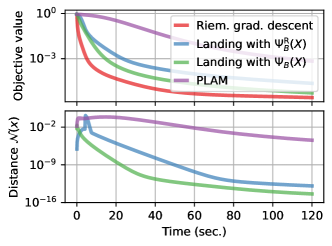
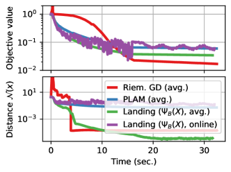
Figure 2: Generalized eigenvalue problem ($n=1000,p=500$).

Figure 3: Stochastic CCA on the split MNIST dataset for $p=5$. An epoch takes roughly $2.5$ sec.

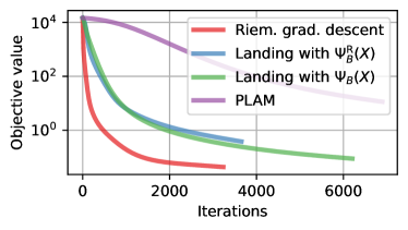
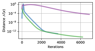
Figure 5: Deterministic computation of the generalized eigenvalue problem with $n=1000,p=500$, the condition number of the two matrices $\kappa=100$. Each algorithm is given a time limit of $120$ seconds.

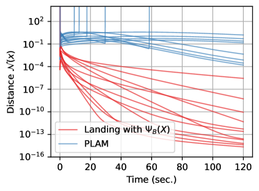
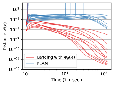
Figure 8: Comparison of the sensitivity to the choice of the step-size $\eta$ and $\omega$ of the landing with $\Psi_{B}(X)$ and the PLAM method (Gao et al., 2022a) in the generalized eigenvalue problem experiment presented in Fig. 3 with $n=1000,p=500$, and the condition number of the two matrices $\kappa=100$. On the right we show log-log scale to better see the effect in earlier iterations. Both parameters are picked as in the experiment for Fig. 3 and multiplied by a scalar from the set $\{0.25,0.75,1.25,1.75\}$ for all possible pair combinations.

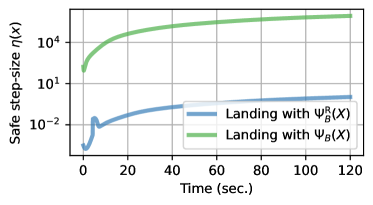
Figure 9: Numerical evaluation of the upper safe-step bound $\eta(X)$ in Lemmma 2.4 per time, which ensures that the iterates stay in ${\mathrm{St}^{\varepsilon}_{B}(p,n)}$, for the two landing methods tested in Fig. 3 with the $L_{\mathcal{N}}$ bounded for the GEVP as in Lemma D.1. We see that the upper bound is only mildly restricting and becomes even less restricting as the iterates come close to a stationary point.

Fig. 3 shows the timings of four methods with fixed stepsize: Riemannian steepest descent with QR-based Cholesky retraction (Sato & Aihara, 2019), the two landing methods with either $\Psi^{\mathrm{R}}_{B}(X)$ and $\Psi_{B}(X)$ in Prop. 3.2, and the PLAM method (Gao et al., 2022a). The landing method with $\Psi_{B}(X)$ converges the fastest in terms of time, due to its cheap per-iteration computation, which is also demonstrated in Fig. 5 and Fig. 7 in the appendices. It can be also observed, that the landing method with $\Psi_{B}(X)$ is more robust to the choice of parameters $\eta$ and $\omega$ compared to PLAM, which we show in Fig. 8 and Fig. 10 in the appendices, and is in line with the equivalent observations previously made for the orthogonal manifold (Ablin & Peyré, 2022, Fig. 9). In Fig. 9 in the appendices we track numerically the value of the upper bound $\eta(X)$ of the safe stepsize in Lemma 2.4, which shows that it is mildly restricting at the start and becomes relaxed as the iterations approach a critical point.

Stochastic CCA and ICA.

For stochastic CCA, we use the standard benchmark problem, in which the MNIST dataset is split in half by taking left and right halves of each image, and compute the top-$p$ canonical correlation components by solving (4).

The stochastic ICA is performed by solving

$$\min_{X\in\mathbb{R}^{n\times n}}\frac{1}{N}\sum_{i=1}^{N}\sum_{j=1}^{n}\sigma([AX]_{i,j}),\,\mathrm{s.t.}\,X\in\mathrm{St}_{\frac{1}{N}A^{\top}A}(n,n)$$

where $\sigma(x)=\log(\mathrm{cosh}(x))$ is performed elementwise and $\sigma^{\prime}(x)=\mathrm{tanh}(x)$. We generate the matrix $A$ as $A=SB^{\top}$, where $S\in\mathbb{R}^{N\times n}$ is a random orthogonal $n\times n$ mixing matrix, the number of samples $N=100\,000$ and $n=10$.

Fig. 3 and Fig. 4 show the timings for the Riemannian gradient descent with rolling averaged covariance matrix and the landing algorithm with $\Psi_{B}(X)$ in its online and averaged form for the CCA and the ICA experiment respectively. The averaged methods keep track of the covariance matrices during the first pass through the dataset, which is around $3$ sec. and $0.6$ sec. respectively, after which they have the exact fully sampled covariance matrices. The online methods have always only the sampled estimate with the batch size of $r=512$. The stepsize for all the methods is $\eta=0.1$ and $\omega=1$; in practice, the hyperparameters can be picked by grid-search as is common for stochastic optimization methods.

The online landing method outperforms the averaged Riemannian gradient descent in the online setting in terms of the objective value after only a few passes over the data, e.g. at the $3$ sec. mark and the $0.6$ sec. mark respectively, which corresponds to the first epoch, at which point each sample appeared just once. After the first epoch, the rolling avg. methods get the advantage of the exact fully sampled covariance matrix and, consequently, have better distance $\mathcal{N}(X)$, but at the cost of requiring $\mathcal{O}(n^{2})$ memory for the full covariance matrix. The online method does not form $B$ and requires only $\mathcal{O}(np)$ memory. The behavior is also consistent when $p=10$ as shown in Fig. 6 in the appendices.

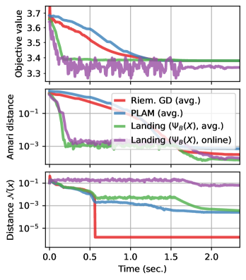
Figure 4: Stochastic ICA on the synthetic dataset for $n=10$.

5 Conclusion

We extend the theory of the landing method from the Stiefel manifold to the general case of a smooth constraint $h(x)=0$. We improve the existing analysis by using a smooth Lagrangian function, which allows us to also consider situations when we have only random estimates of the manifold, and we wish our iterates to be in the feasible set defined by an expectation. We show that random generalized Stiefel manifold, which is central to problems such as stochastic CCA, ICA, and the GEVP, falls into the category of random manifold constraints and derive specific bounds for it. The analysis yields improved complexity bounds for stochastic GEVP when the matrices are well-conditioned.

Acknowledgments

This work was supported by the Fonds de la Recherche Scientifique-FNRS under Grant no T.0001.23. Simon Vary is a beneficiary of the FSR Incoming Post-doctoral Fellowship.

Impact statement.

This paper presents theoretical work which aims to advance the field of machine learning. There is no broad impact other than the consequences discussed in the paper.

Appendix A Summary of retractions on the generalized Stiefel manifold

For an update to a matrix $X\in{\mathrm{St}_{B}(p,n)}$ following the direction $Z\in\mathbb{R}^{n\times p}$ there are several ways to compute a retraction.

• The Polar decomposition (Yger et al., 2012) uses

  $$\mathrm{Retr}_{\mathrm{St}_{B}}(X,Z)=(X+Z)\left(I_{p}+Z^{\top}BZ\right)^{-1/2},$$ (15)

  where it is necessary to compute matrix product and a matrix square root inverse, amounting to $\mathcal{O}(n^{2}p)$ flops.

• Mishra & Sepulchre (2016) observed that the aforementioned polar decomposition can be expressed as $UV^{\top}$ in terms of an SVD-like decomposition of $X+Z=U\Sigma V^{\top}$, where $U,V$ are orthogonal in respect to $B$-inner product, whose main cost is the eigendecomposition of $(X+Z)^{\top}B(X+Z)$.

• Recently, (Sato & Aihara, 2019) proposed the Cholesky-QR based retraction

  $$\mathrm{Retr}_{\mathrm{St}_{B}}(X,Z)=(X+Z)R^{-1},$$ (16)

  where $R\in\mathbb{R}^{p\times p}$ comes from Cholesky factorization of $R^{\top}R=(X+Z)^{\top}B(X+Z)$. The flops required for the computation amount to $\mathcal{O}(n^{2}p)$, which comes from the matrix multiplications, the Cholesky factorization of an $p\times p$ matrix, and finally, the inverse multiplication by a small triangular $p\times p$ matrix requires $\mathcal{O}(p^{3})$ to form and $\mathcal{O}(np^{2})$ to multiply with.

Appendix B Additional experiments and figures

For the experiment showed in Fig. 3, we generate the matrix $A\in\mathbb{R}^{n\times n}$ to have equidistant eigenvalues $\lambda(A)_{i}\in[1/\kappa,1]$ and $B\in\mathbb{R}^{n\times n}$ has exponentially decaying eigenvalues $\lambda(B)_{i}\in[1/\kappa,1]$. We pick the step-size $\eta$ parameter to be $\eta=0.01$ for the Riemannian gradient descent, the landing with $\Psi_{B}^{\mathrm{R}}(X)$, and PLAM, and $\eta=200$ for the landing with $\Psi_{B}(X)$ and we run a grid-search with step-sizes $c\eta$, where $c\in[1/4,1/2,1,2,4,8]$. The normalizing parameter $\omega$ is chosen to be $\omega=10^{5}$ for the landing with $\Psi_{B}^{\mathrm{R}}(X)$, $\omega=0.1$ for the landing with $\Psi_{B}(X)$, and $\omega=200$ for PLAM.

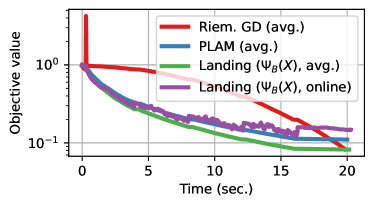
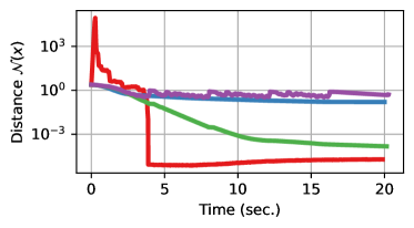
Figure 6: Stochastic canonical correlation analysis on the split MNIST dataset for $p=10$ canonical components.

(a) $\eta/8$

(b) $\eta/4$

(c) $\eta/2$

(d) $2\eta$

(e) $4\eta$.

Figure 10: Robustness of the convergence towards the ${\mathrm{St}_{B}(p,n)}$ for the landing with $\Psi_{B}(X)$ in the experiment for Fig. 3 based on the multiplied perturbations of $\eta$ and $\omega$ parameters with the values from $\{1/8,1/4,1/2,2,4\}$.

Appendix C Proofs for Section 2

C.1 Proof of Proposition 2.2

Proof.

It follows from the definition (7) and $\mathrm{D}h(x)\mathrm{D}h(x)^{*}\left(\mathrm{D}h(x)^{*}\right)^{\dagger}=\mathrm{D}h(x)$ that $\mathrm{D}h(x)({\mathrm{grad}}f(x))=0$, which implies the first condition in Definition 2.1 holds, i.e., $\left\langle{\mathrm{grad}}f(x),\,v\right\rangle=0$ for all $v\in\mathrm{span}(\mathrm{D}h(x)^{*})$. Since $\mathrm{D}h(x)^{*}\left(\mathrm{D}h(x)^{*}\right)^{\dagger}\nabla f(x)\in\mathrm{span}(\mathrm{D}h(x)^{*})$, we have

$$\|{\mathrm{grad}}f(x)\|^{2} =\left\langle{\mathrm{grad}}f(x),\,{\mathrm{grad}}f(x)\right\rangle$$

$$=\left\langle{\mathrm{grad}}f(x),\,\nabla f(x)-\mathrm{D}h(x)^{*}\left(\mathrm{D}h(x)^{*}\right)^{\dagger}\nabla f(x)\right\rangle$$

$$=\left\langle{\mathrm{grad}}f(x),\,\nabla f(x)\right\rangle,$$

which verifies the second condition with $\rho=1$ and the third condition with ${\mathrm{grad}}f(x)=0$ for a critical point $x\in\mathcal{M}$. ∎

C.2 Proof of Lemma 2.4

Proof.

For ease of notation we denote the current iterate $x$ and the subsequent iterate as $\tilde{x}=x-\eta\Lambda(x)$. From $L_{\mathcal{N}}$-Lipschitz of $\mathcal{N}$ we have

$$\mathcal{N}(\tilde{x}) \leq\mathcal{N}(x)+\left\langle\nabla\mathcal{N}(x),\,-\eta\Lambda(x)\right\rangle+\frac{\eta^{2}L_{\mathcal{N}}}{2}\|\Lambda(x)\|^{2}$$ (17)

$$=\mathcal{N}(x)-\eta\omega\|\nabla\mathcal{N}(x)\|^{2}+\frac{\eta^{2}L_{\mathcal{N}}}{2}\|\Lambda(x)\|^{2},$$ (18)

where in the first line we use that $\mathcal{N}(x)$ has Lipschitz gradient with the constants $L_{\mathcal{N}}$ for $x$ in the safe-region. To guarantee $h(\tilde{x})\leq\varepsilon$, we have to ensure that

$$\mathcal{N}(x)-\eta\omega\|\nabla\mathcal{N}(x)\|^{2}+\frac{\eta^{2}L_{\mathcal{N}}}{2}\|\Lambda(x)\|^{2}\leq\frac{\varepsilon^{2}}{2}.$$ (19)

Solving the quadratic inequality in (19) for the positive root $\eta>0$ yields the results. ∎

C.3 Proof of Lemma 2.5

Proof.

Assume that $\|\nabla\mathcal{N}(x)\|\geq\bar{C}_{h}\|h(x)\|$ is lower bounded in $\mathcal{M}^{\varepsilon}$. We proceed to lower bound the numerator of the safe-step size bound in Lemma 2.4 by making it independent of $x\in\mathcal{M}^{\varepsilon}$ as follows

$$\omega\|\nabla\mathcal{N}(x)\|^{2}+ \sqrt{\omega^{2}\|\nabla\mathcal{N}(x)\|^{4}+L_{\mathcal{N}}\|\Lambda(x)\|^{2}(\varepsilon^{2}-\|h(x)\|^{2})}$$

$$\geq\omega\bar{C}_{h}^{2}\|h(x)\|^{2}+\sqrt{\omega^{2}\bar{C}_{h}^{4}\|h(x)\|^{4}+L_{\mathcal{N}}\|\Psi(x)\|^{2}\left(\varepsilon^{2}-\|h(x)\|^{2}\right)}$$ (20)

$$\geq\omega\bar{C}_{h}^{2}\|h(x)\|^{2}\left(1+\frac{1}{\sqrt{2}}\right)+\frac{1}{\sqrt{2}}\|\Psi(x)\|\sqrt{L_{\mathcal{N}}\left(\varepsilon^{2}-\|h(x)\|^{2}\right)}$$ (21)

$$\geq\sqrt{\frac{L_{\mathcal{N}}}{2}}\|\Psi(x)\|(\varepsilon-\|h(x)\|)+\left(1+\frac{1}{\sqrt{2}}\right)\omega\bar{C}_{h}^{2}\|h(x)\|^{2}$$ (22)

where the first inequality comes from using bounds from Assumption 2.2, the second inequality comes from $\sqrt{a+b}\geq(\sqrt{a}+\sqrt{b})/\sqrt{2}$ for $a,b\geq 0$, and the final inequality from the fact that $\sqrt{a-b}\geq\sqrt{a}-\sqrt{b}$ for $a,b\geq 0$ and $a\geq b$. As a result we have that the upper bound in Lemma 2.4 is lower-bounded by

$$\eta(x)\geq\frac{\sqrt{\frac{L_{\mathcal{N}}}{2}}\|\Psi(x)\|(\varepsilon-\|h(x)\|)+\left(1+\frac{1}{\sqrt{2}}\right)\omega\bar{C}_{h}^{2}\|h(x)\|^{2}}{L_{\mathcal{N}}\left(\|\Psi(x)\|^{2}+\omega^{2}C_{h}^{2}\|h(x)\|^{2}\right)},$$ (23)

using the fact that $\|\Lambda(x)\|^{2}=\|\Psi(x)\|^{2}+\omega^{2}\|\nabla\mathcal{N}(x)\|^{2}$ and $\|\nabla\mathcal{N}(x)\|^{2}\leq C_{h}^{2}\|h(x)\|^{2}$. Since the minimum of (23) in terms of $\|h(x)\|\in[0,\varepsilon]$ is on the boundary, when $\|h(x)\|=0$ or $\|h(x)\|=\varepsilon$, we can further lower bound the safe step size as

$$\eta(x)\geq\min\left\{\frac{\varepsilon}{\sqrt{2L_{\mathcal{N}}}C_{\Psi}},\,\frac{\omega\bar{C}_{h}^{2}\varepsilon^{2}}{L_{\mathcal{N}}(C_{\Psi}^{2}+\omega^{2}C_{h}\varepsilon^{2})}\right\}$$ (24)

where we used for the minimum at $\|h(x)\|=0$ and the bound $\sup_{x\in\mathcal{M}^{\varepsilon}}\|\Psi(x)\|\leq C_{\Psi}$. ∎

C.4 Proof of Lemma 2.6

Proof.

The inner product has two parts

$$\left\langle\nabla\mathcal{L}(x),\,\Lambda(x)\right\rangle =\mathrm{D}\mathcal{L}(x)[\Lambda(x)]$$

$$=\mathrm{D}\mathcal{L}(x) [\Psi(x)]+\omega\mathrm{D}\mathcal{L}(x)[\nabla\mathcal{N}(x)].$$ (25)

We expand the first term of the right hand side of (25) as

$$\mathrm{D}\mathcal{L}(x)[\Psi(x)] =\left\langle\nabla f(x),\,\Psi(x)\right\rangle-\left\langle(\mathrm{D}h(x)^{*})^{\dagger}\nabla f(x),\,\mathrm{D}h(x)\Psi(x)\right\rangle$$

$$\qquad-\left\langle\mathrm{D}\lambda(x)[\Psi(x)],\,h(x)\right\rangle+2\beta\left\langle\nabla\mathcal{N}(x),\,\Psi(x)\right\rangle$$

$$=\left\langle\nabla f(x),\,\Psi(x)\right\rangle-\left\langle\mathrm{D}\lambda(x)[\Psi(x)],\,h(x)\right\rangle$$ (26)

where we use that $\nabla\|h(x)\|^{2}=2\nabla\mathcal{N}(x)$ and that the second and the third term are zero due to the orthogonality of $\Psi(x)$ with the span of $\mathrm{D}h(x)^{*}$. We expand the second term of the right hand side of in (25) as

$$\mathrm{D}\mathcal{L}(x)[\nabla\mathcal{N}(x)] =\left\langle\nabla f(x),\,\nabla\mathcal{N}(x)\right\rangle-\left\langle(\mathrm{D}h(x)^{*})^{\dagger}\nabla f(x),\,\mathrm{D}h(x)\nabla\mathcal{N}(x)\right\rangle$$

$$\qquad-\left\langle\mathrm{D}\lambda(x)[\nabla\mathcal{N}(x)],\,h(x)\right\rangle+2\beta\|\nabla\mathcal{N}(x)\|^{2}$$

$$=\left\langle(I_{n}-\mathrm{D}h(x)^{*}(\mathrm{D}h(x)^{*})^{\dagger})\nabla f(x),\,\nabla\mathcal{N}(x)\right\rangle$$

$$\qquad-\left\langle\mathrm{D}\lambda(x)[\nabla\mathcal{N}(x)],\,h(x)\right\rangle+2\beta\|\nabla\mathcal{N}(x)\|^{2}$$

$$=-\left\langle\mathrm{D}\lambda(x)[\nabla\mathcal{N}(x)],\,h(x)\right\rangle+2\beta\|\nabla\mathcal{N}(x)\|^{2},$$ (27)

where in the second equality we move the adjoint $\mathrm{D}h(x)^{*}$ in the second inner product to the left side and join it with the first inner product. The third equality comes from the fact that due to the projection of $\nabla f(x)$ on the orthogonal complement of $\mathrm{D}h(x)^{*}$ and $\nabla\mathcal{N}(x)=\mathrm{D}h(x)^{*}h(x)$ are orthogonal.

Joining the two components (26) and (27) together we get

$$\langle\nabla\mathcal{L}(x),\,\Lambda(x)\rangle =\left\langle\nabla f(x),\,\Psi(x)\right\rangle-\left\langle\mathrm{D}\lambda(x)[\Lambda(x)],\,h(x)\right\rangle+2\beta\omega\|\nabla\mathcal{N}(x)\|^{2}$$

$$\geq\rho\|\Psi(x)\|^{2}-C_{\lambda}\left(\|\Psi(x)\|+\omega\|\nabla\mathcal{N}(x)\|\right)\|h(x)\|+2\beta\omega\|\nabla\mathcal{N}(x)\|^{2}$$

$$\geq\rho\|\Psi(x)\|^{2}+\omega(2\beta C_{h}-C_{\lambda})C_{h}\|h(x)\|^{2}-C_{\lambda}\|\Psi(x)\|\|h(x)\|$$

$$\geq\rho\|\Psi(x)\|^{2}+\omega(2\beta C_{h}-C_{\lambda})C_{h}\|h(x)\|^{2}-C_{\lambda}\left(\alpha\|\Psi(x)\|^{2}+\alpha^{-1}\|h(x)\|^{2}\right)$$

$$\geq\left(\rho-C_{\lambda}\alpha\right)\|\Psi(x)\|^{2}+(2\omega\beta C_{h}^{2}-\omega C_{h}C_{\lambda}-\alpha^{-1}C_{\lambda})\|h(x)\|^{2}$$

$$\geq\frac{\rho}{2}\left(\|\Psi(x)\|^{2}+\|h(x)\|^{2}\right)$$

where the first inequality comes from $\left\langle\nabla f(x),\,\Psi(x)\right\rangle\geq\rho\|\Psi(x)\|^{2}$ in Def. 2.1 combined with the bound $\sup_{x\in\mathcal{M}^{\varepsilon}}\|\mathrm{D}\lambda(x)\|\leq C_{\lambda}$ and the triangle inequality, the second inequality comes from bounding $\|\nabla\mathcal{N}(x)\|\leq C_{h}\|h(x)\|$ using Assumption 2.2 and rearranging terms, the third inequality comes from using the AG-inequality $\sqrt{ab}\leq(a+b)/2$ with $a=\alpha\|h(x)\|$ and $b=\alpha^{-1}\|\Psi(x)\|$ for an arbitrary $\alpha>0$, in the fourth inequality we only rearrange terms, and finally, in the fifth inequality we choose $\alpha=\rho/(2C_{\lambda})$ and use that $\beta=(\frac{\rho}{4C_{h}^{2}}+\frac{C_{\lambda}}{2C_{h}}+\frac{C_{\lambda}^{2}}{C_{h}^{2}})/\omega$. ∎

C.5 Proof of Theorem 2.7

Proof.

Due to $x_{0}\in\mathcal{M}^{\varepsilon}$ and the step size being smaller than the bound in Lemma 2.5, we have that all iterates remain in the safe region $x^{k}\in\mathcal{M}^{\varepsilon}$. By smoothness of Fletcher’s augmented Lagrangian and the fact that the segment $[x^{k},x^{k+1}]\in{\mathrm{St}^{\varepsilon}_{B}(p,n)}$ by $\eta$ being a safe-stepsize from Lemma 2.4, we can expand

$$\mathcal{L}(x^{k+1}) \leq\mathcal{L}(x^{k})-\eta\left\langle\Lambda(x^{k}),\,\nabla\mathcal{L}(x^{k})\right\rangle+\frac{L_{\mathcal{L}}\eta^{2}}{2}\|\Lambda(x^{k})\|^{2}$$ (28)

$$\leq\mathcal{L}(x^{k})-\frac{\eta\rho}{2}\left(\|\Psi(x^{k})\|^{2}+\omega^{2}\|h(x^{k})\|^{2}\right)+\frac{L_{\mathcal{L}}\eta^{2}}{2}\|\Lambda(x^{k})\|^{2}$$ (29)

$$\leq\mathcal{L}(x^{k})-\frac{\eta}{2}\Big{(}\left(\rho-L_{\mathcal{L}}\eta\right)\|\Psi(x^{k})\|^{2}+\omega^{2}\left(\rho-\eta L_{\mathcal{L}}C_{h}^{2}\right)\|h(x^{k})\|^{2}\Big{)},$$ (30)

where in the second inequality we used the results of Lemma 2.6, and in the third inequality we use the bound on $\|\nabla\mathcal{N}(x)\|\leq C_{h}\|h(x)\|$ by Assumption 2.2. By the step size $\eta<\min{\left\{\frac{\rho}{2L_{\mathcal{L}}},\frac{\rho}{2L_{\mathcal{L}}C_{h}^{2}}\right\}}$ we have

$$\frac{\eta\rho}{4}\|\Psi(x^{k})\|^{2}+\frac{\eta\rho\omega^{2}}{4}\|h(x)\|^{2}\leq\mathcal{L}(x^{k})-\mathcal{L}(x^{k+1}).$$ (31)

Telescopically summing the first $K$ terms gives

$$\frac{\eta\rho}{4}\sum_{k=0}^{K}\|\Psi(x^{k})\|^{2}+\frac{\eta\rho\omega^{2}}{4}\sum_{k=0}^{K}\|h(x)\|^{2}\leq\mathcal{L}(x^{0})-\mathcal{L}(x^{K+1})\leq\mathcal{L}(x^{0})-\mathcal{L}^{*},$$

which implies that the inequalities hold individually also

$$\frac{\eta\rho}{4}\sum_{k=0}^{K}\|\Psi(x^{k})\|^{2}\leq\mathcal{L}(x^{0})-\mathcal{L}^{*}\qquad\text{and}\qquad\frac{\eta\rho\omega^{2}}{4}\sum_{k=0}^{K}\|h(x)\|^{2}\leq\mathcal{L}(x^{0})-\mathcal{L}^{*}.$$

∎

C.6 Proof of Theorem 2.8

Proof.

Let $x^{k+1}=x^{k}-\eta\tilde{\Lambda}(x^{k})$, where we denote $\tilde{\Lambda}(x^{k})=\Lambda(x^{k})+\tilde{E}(x^{k},\Xi^{k})$ the unbiased estimator of the landing update, and we assume that the line segment between the iterates remain within $\mathcal{M}^{\varepsilon}$. By the Lipschitz continuity of the gradient of Fletcher’s augmented Lagrangian inside of $\mathcal{M}^{\varepsilon}$, we have

$$\mathbb{E} \left[\mathcal{L}(x^{k+1})\right]\leq\mathbb{E}\Big{[}\mathcal{L}(x^{k})-\eta\left\langle\tilde{\Lambda}(x^{k}),\,\nabla\mathcal{L}(x^{k})\right\rangle+\frac{L_{\mathcal{L}}\eta^{2}}{2}\|\tilde{\Lambda}(x^{k})\|^{2}\Big{]}$$

$$\leq\mathcal{L}(x^{k})-\eta\left\langle\Lambda(x^{k}),\,\nabla\mathcal{L}(x^{k})\right\rangle+\frac{L_{\mathcal{L}}\eta^{2}}{2}\left(\|\Lambda(x^{k})\|^{2}+\gamma^{2}\right)$$

$$\leq\mathcal{L}(x^{k})-\frac{\eta\rho}{2}\left(\|\Psi(x^{k})\|^{2}+\omega^{2}\|h(x)\|^{2}\right)+\frac{L_{\mathcal{L}}\eta^{2}}{2}\left(\|\Lambda(x^{k})\|^{2}+\gamma^{2}\right)$$

$$\leq\mathcal{L}(x^{k})+\frac{L_{\mathcal{L}}\eta^{2}}{2}\gamma^{2}-\frac{\eta}{2}\left(\left(\rho-L_{\mathcal{L}}\eta\right)\|\Psi(x^{k})\|^{2}+\omega^{2}\left(\rho-\eta L_{\mathcal{L}}C_{h}^{2}\right)\|h(x^{k})\|^{2}\right),$$

where the first inequality comes from taking an expectation of the Lipschitz-continuity of $\mathcal{L}(x)$, in the second inequality we take the expectation inside of the inner product using the fact that $\tilde{\Lambda}(x^{k})$ is zero-centered and has bounded variance, the third and the last inequality comes as a consequence of Lemma 2.6. By the step size being smaller than $\eta<\min{\left\{\frac{\rho}{2L_{\mathcal{L}}},\frac{\rho}{2L_{\mathcal{L}}C_{h}^{2}}\right\}}$ we have that

$$\frac{\eta\rho}{4}\|\Psi(x^{k})\|^{2}+\frac{\eta\rho\omega^{2}}{4}\|h(x)\|^{2}\leq\mathcal{L}(x^{k})-\mathcal{L}(x^{k+1})+\frac{L_{\mathcal{L}}\eta^{2}}{2}\gamma^{2}$$

Telescopically summing the first $K$ terms gives

$$\frac{\eta\rho}{4}\sum_{k=1}^{K}\|\Psi(x^{k})\|^{2}+\frac{\eta\rho\omega^{2}}{4}\sum_{k=0}^{K}\|h(x^{k})\|^{2} \leq\mathcal{L}(x^{0})-\mathcal{L}(x^{K+1})+\frac{L_{\mathcal{L}}\eta^{2}\gamma^{2}}{2}\sum_{k=0}^{K}(1+k)^{-1}$$ (32)

$$\leq\mathcal{L}(x^{0})-\mathcal{L}^{*}+\frac{L_{\mathcal{L}}\eta^{2}\gamma^{2}}{2}\log(K)$$

which implies that the inequalities hold also individually

$$\inf_{k\leq K}\|\Psi(x^{k})\|^{2} \leq\frac{4}{\rho\eta_{0}\sqrt{K}}\left(\mathcal{L}(x^{0})-\mathcal{L}^{*}+\frac{\eta_{0}L_{\mathcal{L}}\gamma^{2}}{2}\log(K)\right),$$

$$\inf_{k\leq K}\|h(x^{k})\|^{2} \leq\frac{4}{\rho\omega^{2}\eta_{0}\sqrt{K}}\left(\mathcal{L}(x^{0})-\mathcal{L}^{*}+\frac{\eta_{0}L_{\mathcal{L}}\gamma^{2}}{2}\log(K)\right),$$

where we used that $\inf_{k\leq K}\|\Psi(x^{k})\|^{2}\leq\sum_{k=0}^{K}\eta_{k}\|\Psi(x^{k})\|^{2}\left(\sum_{k=0}^{K}\eta_{k}\right)^{-1}$ and the fact that $\sum_{k\leq K}\eta_{k}\geq\eta_{0}\sqrt{K}$. ∎

Appendix D Proofs for Section 3

D.1 Specific forms of $\mathrm{D}h(x),\lambda(X)$ for ${\mathrm{St}_{B}(p,n)}$

We begin by showing the specific form of the formulations derived in the previous section for the case of the generalized Stiefel manifold. Differentiating the generalized Stiefel constraint yields $\mathrm{D}h(X)[V]=X^{\top}BV+V^{\top}BX$ and the adjoint is derived as

$$\left\langle\mathrm{D}h(X)^{*}[V],\,W\right\rangle=\left\langle V,\,\mathrm{D}h(X)[W]\right\rangle =\left\langle V,\,W^{T}BX+X^{T}BW\right\rangle=\left\langle 2BX{\mathrm{sym}}(V),\,W\right\rangle,$$ (33)

as such we have that $\mathrm{D}h(X)^{*}[V]=2BX{\mathrm{sym}}(V)$. Consequently

$$\mathrm{D}h(X)\mathrm{D}h(X)^{*}[V]=2{\mathrm{sym}}(V)X^{\top}B^{2}X+2X^{\top}B^{2}X{\mathrm{sym}}(V),$$ (34)

and the Lagrange multiplier $\lambda(X)$ is defined in the case of the generalized Stiefel manifold as the solution to the following Lyapunov equation

$$2\lambda(X)X^{\top}B^{2}X+2X^{\top}B^{2}X\lambda(X)=X^{\top}B\nabla f(X)+\nabla f(X)^{\top}BX.$$ (35)

Importantly, due to $\lambda(X)$ being the unique solution to the linear equation and $\nabla f(X)$ being smooth, $\lambda(X)$ is also smooth with respect to $X$, and as a smooth function defined over a compact set ${\mathrm{St}^{\varepsilon}_{B}(p,n)}$, its operator norm is bounded $\sup_{X\in{\mathrm{St}^{\varepsilon}_{B}(p,n)}}\|\mathrm{D}\lambda(X)\|_{F}\leq C_{\lambda}$ as required by Assumption 2.3.

D.2 Proof of Proposition 3.1

Proof.

For $\|X^{\top}BX-I_{p}\|_{F}\leq\varepsilon$, $X=U\Sigma V^{\top}$ be the singular value decomposition of $X$, and $QDQ^{\top}$ be the spectral decomposition of $B$. We then have

$$\varepsilon^{2}\geq\|X^{\top}BX-I_{p}\|_{\mathrm{F}}^{2} =\|\Sigma U^{\top}QD(U^{\top}Q)^{\top}\Sigma-I_{p}\|_{\mathrm{F}}^{2}$$ (36)

where $\beta_{i},\sigma_{i}$ are the positive eigenvalues of $B$ and the singular values of $X$ respectively in the decreasing order. This implies that

$$\sqrt{(1-\varepsilon)/\beta_{1}}\leq\sigma_{i}\leq\sqrt{(1+\varepsilon)/\beta_{n}}.$$ (37)

The above bound gives that the singular values of $\mathrm{D}h(X)^{*}=2BX$ are in the interval $[2\sqrt{(1-\varepsilon)\kappa^{-1}},2\sqrt{(1+\varepsilon)\kappa}]$ which in turn gives the constants $C_{h},\bar{C}_{h}$. ∎

Lemma D.1 (Lipschitz constants for the generalized eigenvalue problem).

Let $f=-\frac{1}{2}\operatorname{Tr}(X^{\top}AX)$ and $\mathcal{N}(X)=\|X^{\top}BX-I_{p}\|_{F}^{2}$ as in the optimization problem corresponding to the generalized eigenvalue problem. We have that, for $X\in{\mathrm{St}^{\varepsilon}_{B}(p,n)}$, the Lipschitz constant for $\nabla\mathcal{N}$ is $L_{\mathcal{N}}=\beta_{1}\varepsilon+2(1+\varepsilon)\kappa$ and the for $\nabla f$ is $L_{f}=\alpha_{1}$ where $\alpha_{1}$ is the largest eigenvalue of $A$.

Proof.

Take $X,Y\in{\mathrm{St}_{B}(p,n)}$, we have that $\nabla\mathcal{N}(X)=BX(X^{\top}BX)$, thus

$$\nabla\mathcal{N}(X)-\nabla\mathcal{N}(Y) =B\left(X(X^{\top}BX-I_{p})-Y(Y^{\top}BY)\right)$$ (38)

$$=B(X-Y)(X^{\top}BX-I_{p})+B(X^{\top}BX-Y^{\top}BY)$$ (39)

$$=B(X-Y)(X^{\top}BX-I_{p})+BY(X-Y)^{\top}BX+BYY^{\top}B(X-Y)$$ (40)

Taking the Frobenius norm and by the triangle inequality we get

$$\|\nabla\mathcal{N}(X)-\nabla\mathcal{N}(Y)\| \leq\|X-Y\|\left(\|B\|\|X^{\top}BX-I_{p}\|+\|B\|^{2}\|X\|\|Y\|+\|B\|^{2}\|Y\|^{2}\right)$$ (41)

$$\leq\|X-Y\|(\beta_{1}\varepsilon+2(1+\varepsilon)\kappa),$$ (42)

where we used the fact that $X\in{\mathrm{St}^{\varepsilon}_{B}(p,n)}$ and we have that $\|X\|_{2}\leq\sqrt{(1+\varepsilon)\kappa}$ and the same for $Y\in{\mathrm{St}^{\varepsilon}_{B}(p,n)}$.

When $f=\frac{1}{2}\operatorname{Tr}(X^{\top}AX)$, we have that $\|\nabla f(X)-\nabla f(Y)\|\leq\|A\|_{2}\|X-Y\|$.

∎

D.3 Proof of Proposition 3.2

Proof.

For ease of notation we denote $G=\nabla f(X)\in\mathbb{R}^{n\times p}$. The first property Definition 2.1 (i) comes from

$$\left\langle{\mathrm{skew}}(GX^{\top}B)BX,\,BXS\right\rangle=0,$$ (43)

which holds for a symmetric matrix $S$, since a skew-symmetric matrix is orthogonal in the trace inner product to a symmetric matrix,

The second property (ii) is a consequence of the following

$$\left\langle\Psi_{B}(X),\,G\right\rangle =\left\langle{\mathrm{skew}}(GX^{T}B)BX,\,G\right\rangle$$

$$= \|{\mathrm{skew}}(GX^{T}B)\|_{\mathrm{F}}^{2}\geq\frac{1}{(1+\varepsilon)\kappa}\|\Psi_{B}(X)\|_{\mathrm{F}}^{2},$$

where we use the bounds on $\|BX\|_{2}\leq\sqrt{(1+\varepsilon)\kappa}$ derived in the proof of Proposition 3.1 in (37) for $\kappa=\beta_{1}/\beta_{n}$ the condition number of $B$.

To show the third property (iii), we first consider a critical point $X\in{\mathrm{St}_{B}(p,n)}$, for which must hold

$$G=BXS,$$ (44)

for some $S\in{\mathrm{sym}}(p)$ due to the constraints being symmetric and that $X^{\top}BX=I_{p}$ by feasibility. We have that at the critical point defined in (44), the relative descent direction is

$$\Psi_{B}(X) ={\mathrm{skew}}(GX^{\top}B)BX={\mathrm{skew}}(BXSX^{\top}B)BX=0,$$ (45)

where the second equality is the consequence of (44) and the third equality comes from the fact that $BXSX^{\top}B$ is symmetric.

To show the other side of the implication, that $\Psi_{B}(X)=0$ combined with feasibility imply that $X$ is a critical point, we consider

$$0=\Psi(x)={\mathrm{skew}}(GX^{\top}B)BX=GX^{\top}B^{2}X-BXG^{\top}BX$$ (46)

which, since $X^{\top}B^{2}X\in\mathbb{R}^{p\times p}$ is invertible, is equivalent to

$$G=BXG^{\top}BX\left(X^{\top}B^{2}X\right)^{-1}.$$ (47)

For $X$ to be a critical point, we must have that $G^{\top}BX\left(X^{\top}B^{2}X\right)^{-1}$ is symmetric:

$$G^{\top}BX\left(X^{\top}B^{2}X\right)^{-1}=\left(X^{\top}B^{2}X\right)^{-1}X^{\top}BG,$$ (48)

which, after multiplying by $\left(X^{\top}B^{2}X\right)$ from both sides and rearranging terms, is equivalent to

$$X^{\top}B{\mathrm{skew}}(BXG^{\top})BX=0,$$ (49)

that is true from multiplying (46) by $X^{\top}B$ from the left.

For the other choice of relative gradient $\Psi_{B}^{\mathrm{R}}(X)={\mathrm{skew}}(B^{-1}GX^{\top})BX$, letting $M=B^{-1}GX^{\top}$, we find

$$\langle\Psi_{B}^{\mathrm{R}}(X),G\rangle =\langle{\mathrm{skew}}(M),BMB\rangle$$ (50)

$$=\langle{\mathrm{skew}}(M),{\mathrm{skew}}(BMB)\rangle$$ (51)

$$=\langle{\mathrm{skew}}(M),B{\mathrm{skew}}(M)B\rangle$$ (52)

$$\geq\|{\mathrm{skew}}(M)\|_{\mathrm{F}}^{2}\beta_{n}^{2}$$ (53)

and similarly as before, it holds $\|\Psi_{B}^{\mathrm{R}}(X)\|^{2}\leq\|{\mathrm{skew}}(M)\|_{\mathrm{F}}^{2}(1+\varepsilon)\kappa$ which in turn leads to $\langle\Psi_{B}^{\mathrm{R}}(X),G\rangle\geq\frac{\beta_{n}^{2}}{(1+\varepsilon)\kappa}\|\Psi_{B}\|^{2}$ ∎

D.4 Proof of Proposition 3.3

Proof.

We start by deriving the bound on the variance of the normalizing component $\nabla\mathcal{N}(X)$. Consider $U$ and $V$ to be two independent random matrices taking i.i.d. values from the distribution of $B_{\zeta}$ with variance $\sigma_{B}^{2}$. We have that

$$\mathrm{Var}\left[UX(X^{\top}VX-I_{p})\right]=\mathbb{E}_{U,V}\left[\|UX(X^{\top}VX-I_{p})-BX(X^{\top}BX-I_{p})\|^{2}\right]$$ (54)

Introducing the random marginal $BX(X^{\top}VX-I_{p})$, we further decompose

$$\mathrm{Var}\left[UX(X^{\top}VX-I_{p})\right] =\mathbb{E}_{U,V}\left[\|UX(X^{\top}VX-I_{p})-BX(X^{\top}VX-I_{p})\|^{2}\right]$$ (55)

$$\qquad+\mathbb{E}_{V}\left[\|BX(X^{\top}VX-I_{p})-BX(X^{\top}BX-I_{p})\|^{2}\right].$$ (56)

The first term in the above is upper bounded as

$$\mathbb{E}_{U,V}\left[\|UX(X^{\top}VX-I_{p})-BX(X^{\top}VX-I_{p})\|^{2}\right] \leq\mathbb{E}_{U,V}\left[\|U-B\|_{\mathrm{F}}^{2}\|X(X^{\top}VX-I_{p})\|_{2}^{2}\right]$$ (57)

$$=\sigma_{B}^{2}\mathbb{E}_{V}[\|X(X^{\top}VX-I_{p})\|_{2}^{2}]$$ (58)

and the second is controlled by

$$\mathbb{E}_{V}\left[\|BX(X^{\top}VX-I_{p})-BX(X^{\top}BX-I_{p})\|^{2}\right] =\mathbb{E}_{V}\left[\|BXX^{\top}(V-B)X\|^{2}\right]$$ (59)

$$\leq\sigma_{B}^{2}\|B\|_{2}^{2}\|X\|_{2}^{6}.$$ (60)

Taking things together

$$\mathrm{Var}\left[UX(X^{\top}VX-I_{p})\right] \leq(\mathbb{E}_{V}[\|X(X^{\top}VX-I_{p})\|_{2}^{2}]+\|B\|_{2}^{2}\|X\|_{2}^{6})\sigma_{B}^{2}$$ (61)

$$\leq\left(\frac{1+\varepsilon}{\beta_{n}}\mathbb{E}_{V}[\|X^{\top}VX-I_{p}\|_{2}^{2}]+\frac{(1+\varepsilon)^{3}}{\beta_{n}}\right)\sigma_{B}^{2},$$ (62)

where for the second inequality we can use the bounds on the singular values of $X\in{\mathrm{St}^{\varepsilon}_{B}(p,n)}$.

Similarly, the variance of the first term in the landing is controlled by introducing yet another random variable $G$ that takes values from $\nabla f_{\xi}(X)$. We use the U-statistics variance decomposition twice to get

$$\mathrm{Var}[{\mathrm{skew}} \left(GX^{\top}U\right)VX]=$$

$$\mathbb{E}_{G,U,V}[\|{\mathrm{skew}}((G-\nabla f(X))X^{\top}U)VX\|^{2}]$$

$$+\mathbb{E}_{U,V}[\|{\mathrm{skew}}(\nabla f(X)X^{\top}(U-B))VX\|^{2}]$$

$$+\mathbb{E}_{V}[\|{\mathrm{skew}}(\nabla f(X)X^{\top}B)(V-B)X\|^{2}]$$

which leads to the bound

$$\mathrm{Var}[{\mathrm{skew}} \left(GX^{\top}U\right)VX]\leq\sigma_{G}^{2}\mathbb{E}_{U}[\|UX\|_{2}^{2}]^{2}$$

$$\qquad+\sigma_{B}^{2}(\|\nabla f(X)X^{\top}\|_{2}^{2}\mathbb{E}_{U}[\|UX\|_{2}^{2}]$$

$$\qquad+\|\nabla f(X)X^{\top}B\|_{2}^{2}\|X\|_{2}^{2})$$

Joining the two bounds above, we get the result. ∎

D.5 Proof of Proposition 3.4

Proof.

Same as in the proof of Theorem 2.8, by telescopically summing and averaging the iterates in (32), we arrive at the inequality

$$\frac{\eta\rho}{4K} \sum_{k=1}^{K}\|\Psi_{B}(X^{k})\|^{2}+\frac{\eta\rho\omega^{2}}{4K}\sum_{k=0}^{K}\|h(X^{k})\|^{2}$$

$$\quad\leq\frac{\mathcal{L}(X^{0})-\mathcal{L}(X^{K+1})}{K}+\frac{L_{\mathcal{L}}\eta^{2}\gamma^{2}}{2},$$

which implies also that the following two inequalities hold individually

$$\frac{1}{K}\sum_{k=1}^{K}\|\Psi_{B}(X^{k})\|^{2} \leq\frac{2}{\rho}\left(2\frac{\mathcal{L}(X^{0})-\mathcal{L}(X^{K+1})}{K\eta}+L_{\mathcal{L}}\eta\gamma^{2}\right)$$ (63)

$$\frac{1}{K}\sum_{k=0}^{K}\|h(X^{k})\|^{2} \leq\frac{2}{\rho\omega^{2}}\left(2\frac{\mathcal{L}(X^{0})-\mathcal{L}(X^{K+1})}{K\eta}+L_{\mathcal{L}}\eta\gamma^{2}\right).$$ (64)

In the above we see that the optimal step-size given $K$ iterations is

$$\eta^{*}=\frac{\sqrt{2(L(X^{K+1})-L(X^{0}))}}{\sqrt{KL_{\mathcal{L}}}\gamma}$$ (65)

and the value of the parenthesis on the right-hand side becomes $2\sqrt{2(\mathcal{L}(X^{0})-\mathcal{L}(X^{K}))L_{\mathcal{L}}/K}\gamma$. We thus need

$$K=32L_{\mathcal{L}}\gamma^{2}\frac{\mathcal{L}(X^{0})-\mathcal{L}(X^{K})}{e^{2}\rho^{2}}$$ (66)

iterations to decrease $\inf_{k\leq K}\mathbb{E}\|\Psi(X^{k})\|\leq e$ and similarly, but with extra $\omega^{4}$ in the denominator, for the constraint $\inf_{k\leq K}\mathbb{E}\|h(X^{k})\|\leq e$.

Consider batch $r=1$, since each iteration cost $npr$, we have the following number flops to get $e$-critical point

$$32L_{\mathcal{L}}\gamma^{2}\frac{\mathcal{L}(X^{0})-\mathcal{L}(X^{K})}{e^{2}\rho^{2}}np.$$ (67)

Taking that $L_{\mathcal{L}}=\mathcal{O}(\alpha_{1}+\beta_{1}+\kappa)$ from the previous Lemma D.1 and by the fact that $\rho=\mathcal{O}(1/\kappa)$, we have that we require $\mathcal{O}(\gamma^{2}\kappa^{2}(\kappa+\alpha_{1}+\beta_{1})np/e^{2})$ flops.

It remains to estimate the variance of the landing $\gamma$ in terms of the variances of $\sigma_{G},\sigma_{B}$ using Proposition 3.3, which states:

$$\gamma^{2}\leq\sigma_{G}^{2}p_{B}^{2}\frac{(1+\varepsilon)^{2}}{\beta_{n}^{2}}+\sigma_{B}^{2}\frac{1+\varepsilon}{\beta_{n}}\left(4\Delta(p_{B}+\beta_{1}^{2})+p_{N}+(1+\varepsilon)^{2}\right).$$ (68)

Here we have that $p_{N}=\frac{1+\varepsilon}{\beta_{n}}\sigma_{B}^{2}+\varepsilon$, $\Delta=\sup_{X\in{\mathrm{St}^{\varepsilon}_{B}(p,n)}}\|\nabla f(X)X^{\top}\|^{2}_{2}$, and $p_{B}=\mathbb{E}_{\zeta}\|B_{\zeta}\|_{2}^{2}$ which can be bounded as $p_{B}\leq\beta_{1}^{2}+\sigma_{B}^{2}$. When the variance of the constraint is small and we have that $\sigma_{B}<\beta_{1}$ we get $p_{B}\leq 2\beta_{1}^{2}$ and

$$\gamma^{2}\leq 8\kappa^{2}\beta_{1}^{2}\sigma_{G}^{2}+\left(24\beta_{1}\kappa+10/\beta_{n}\right)\sigma_{B}^{2}+\frac{4}{\beta_{n}}\sigma_{B}^{4}$$ (69)

where we also use that $\varepsilon<1$. This gives an asymptotic bound

$$\gamma^{2}\leq\mathcal{O}\left(\kappa^{2}\beta_{1}^{2}\sigma_{G}^{2}+\left(\beta_{1}\kappa+\beta_{n}^{-1}\right)\sigma_{B}^{2}+\sigma_{B}^{4}/\beta_{n}\right),$$ (70)

leading to the asymptotic number of floating point operations for $e$-criticality to be

$$\left(\kappa^{2}\beta_{1}^{2}\sigma_{G}^{2}+\left(\beta_{1}\kappa+\beta_{n}^{-1}\right)\sigma_{B}^{2}+\sigma_{B}^{4}/\beta_{n}\right)\frac{\kappa^{2}(\kappa+\alpha_{1}+\beta_{1})np}{e^{2}},$$ (71)

where the leading term is

$$\left(\kappa\beta_{1}\sigma_{G}^{2}+\left(1+\beta_{1}^{-2}\right)\sigma_{B}^{2}\right)\frac{\beta_{1}\kappa^{3}(\kappa+\alpha_{1}+\beta_{1})np}{e^{2}}.$$ (72)

∎

Appendix E Riemannian interpretation of $\Psi_{B}^{\mathrm{R}}(X)$ in Prop. 3.2

Similar to the work of (Gao et al., 2022b), we can provide a geometric interpretation of the relative descent direction $\Psi_{B}^{\mathrm{R}}(X)$ as a Riemannian gradient in a canonical-induced metric and the isometry between the standard Stiefel manifold ${\mathrm{St}(p,n)}$ and the generalized Stiefel manifold ${\mathrm{St}_{B}(p,n)}$. Let

$${\mathrm{St}_{B,M}(p,n)}:=\{X:X^{\top}BX=M\},$$

for $B,M\succ 0$, which is the sheet manifold of ${\mathrm{St}_{B}(p,n)}$, and consider a map

$$\Phi_{B,M}:{\mathrm{St}(p,n)}\to{\mathrm{St}_{B,M}(p,n)}:Y\mapsto B^{-\frac{1}{2}}YM^{\frac{1}{2}}.$$

The map $\Phi_{B,M}$ acts as a diffeomorphism of the set of the full rank $\mathbb{R}^{n\times p}$ matrices onto itself and maps the standard Stiefel manifold ${\mathrm{St}(p,n)}$ to the generalized Stiefel manifold ${\mathrm{St}_{B,M}(p,n)}$. It is easy to obtain the tangent space at $X\in{\mathrm{St}_{B,M}(p,n)}$ via the standard definition:

$$\mathrm{T}_{X}{\mathrm{St}_{B,M}(p,n)} =\{\xi\in\mathbb{R}^{n\times p}:\xi^{T}BX+X^{T}B\xi=0\}$$

$$=\{X(X^{T}BX)^{-1}\Omega+B^{-1}X_{\perp}K:\Omega^{T}+\Omega=0,\Omega\in\mathbb{R}^{p\times p},K\in\mathbb{R}^{(n-p)\times p}\}$$

$$=\{WBX:W^{T}+W=0,W\in\mathbb{R}^{n\times n}\}$$

$$=\{\Phi_{B,M}(\zeta):\zeta\in\mathrm{T}_{\Phi^{-1}_{B,M}(X)}{\mathrm{St}(p,n)}\}$$

Consider the canonical metric on the standard Stiefel manifold ${\mathrm{St}(p,n)}$:

$$g_{Y}^{{\mathrm{St}(p,n)}}(Z_{1},Z_{2})=\left\langle Z_{1},\,(I-\frac{1}{2}YY^{T})Z_{2}\right\rangle$$

Using the map $\Phi_{B,M}$, we define the metric $g^{{\mathrm{St}_{B,M}(p,n)}}$ which makes $\Phi_{B,M}$ an isometry as. Hence, we have that this metric is defined as

$$g^{{\mathrm{St}_{B,M}(p,n)}}_{X}(\xi,\zeta) =g^{{\mathrm{St}(p,n)}}_{\Phi_{B}^{-1}(X)}(\Phi_{B}^{-1}(\xi),\Phi_{B}^{-1}(\zeta))$$

$$=\left\langle\xi,\,(B-\frac{1}{2}BX(X^{T}BX)^{-1}X^{T}B)\zeta(X^{T}BX)^{-1}\right\rangle.$$

Consequently, the corresponding normal space of ${\mathrm{St}_{B,M}(p,n)}$ is

$$\mathrm{N}_{X}{\mathrm{St}_{B,M}(p,n)} =\{X(X^{T}BX)^{-1}S:S^{T}=S,S\in\mathbb{R}^{p\times p}\}.$$

The form of the derived tangent and normal spaces allow us to derive their projection operators $P_{X}$ and $P_{X}^{\perp}$ respectively as

$$P_{X}^{\perp}(Y) =X(X^{T}BX)^{-1}{\mathrm{sym}}(X^{T}BY),$$

$$P_{X}(Y) =Y-X(X^{T}BX)^{-1}{\mathrm{sym}}(X^{T}BY).$$

Since $\Phi_{B,M}$ is isometric, the Riemannian gradient w.r.t. $g^{{\mathrm{St}_{B,M}(p,n)}}$ can be computed directly by

$${\mathrm{grad}}_{B,M}f(X) =\Phi_{B,M}({\mathrm{grad}}_{Y}f(Y))$$

$$=\Phi_{B,M}({\mathrm{grad}}_{\Phi_{B,M}^{-1}(X)}f(\Phi_{B,M}^{-1}(X)))$$

$$=B^{-\frac{1}{2}}{\mathrm{grad}}_{\Phi_{B,M}^{-1}(X)}f(\Phi_{B,M}^{-1}(X))M^{\frac{1}{2}}$$

$$=2B^{-\frac{1}{2}}{\mathrm{skew}}\left(\nabla f(\Phi_{B,M}^{-1}(X))(\Phi_{B,M}^{-1}(X))^{T}\right)\Phi_{B,M}^{-1}(X)M^{\frac{1}{2}}$$

$$=2{\mathrm{skew}}(B^{-\frac{1}{2}}\nabla f(B^{\frac{1}{2}}XM^{-\frac{1}{2}})M^{-\frac{1}{2}}X^{T})BX$$

$$=2{\mathrm{skew}}(B^{-\frac{1}{2}}B^{-\frac{1}{2}}\nabla f(X)M^{\frac{1}{2}}M^{-\frac{1}{2}}X^{T})BX$$

$$=2{\mathrm{skew}}(B^{-1}\nabla f(X)X^{T})BX.$$

Hence, akin to the work of (Gao et al., 2022b) for the standard Stiefel manifold, we derived the equivalent Riemannian interpretation of $\Psi_{B}^{\mathrm{R}}(X)$ and the landing algorithm for the generalized Stiefel manifold ${\mathrm{St}_{B}(p,n)}$. Note, the formula for $\Psi_{B}^{\mathrm{R}}(X)$ involves computing an inverse of $B$ and thus does not allow a simple unbiased estimator to be used in the stochastic case, as opposed to $\Psi_{B}(X)$.

References

• Ablin & Peyré (2022) Ablin, P. and Peyré, G. Fast and accurate optimization on the orthogonal manifold without retraction. In Proceedings of the 25th International Conference on Artificial Intelligence and Statistics, volume 51, Valencia, Spain, 2022. PMLR.
• Ablin et al. (2023) Ablin, P., Vary, S., Gao, B., and Absil, P.-A. Infeasible Deterministic, Stochastic, and Variance-Reduction Algorithms for Optimization under Orthogonality Constraints. arXiv preprint arXiv:2303.16510, 2023.
• Absil et al. (2007) Absil, P.-A., Baker, C., and Gallivan, K. Trust-Region Methods on Riemannian Manifolds. Foundations of Computational Mathematics, 7(3):303–330, July 2007. doi: 10.1007/s10208-005-0179-9.
• Absil et al. (2008) Absil, P.-A., Mahony, R., and Sepulchre, R. Optimization Algorithms on Matrix Manifolds, volume 36. Princeton University Press, Princeton, NJ, January 2008. ISBN 978-1-4008-3024-4. doi: 10.1515/9781400830244.
• Ahn & Sra (2020) Ahn, K. and Sra, S. From Nesterov’s Estimate Sequence to Riemannian Acceleration. In Proceedings of Machine Learning Research, volume 125, pp.  1–35, 2020.
• Allen-Zhu & Li (2017) Allen-Zhu, Z. and Li, Y. Doubly Accelerated Methods for Faster CCA and Generalized Eigendecomposition. In Proceedings of the 34th International Conference on Machine Learning, volume 70, Sydney, Australia, 2017.
• Arora et al. (2017) Arora, R., Marinov, T. V., Mianjy, P., and Srebro, N. Stochastic approximation for canonical correlation analysis. In Guyon, I., Luxburg, U. V., Bengio, S., Wallach, H., Fergus, R., Vishwanathan, S., and Garnett, R. (eds.), Advances in Neural Information Processing Systems, volume 30. Curran Associates, Inc., 2017.
• Bertsekas (1982) Bertsekas, D. P. Constrained Optimization and Lagrange Multiplier Methods. Athena Scientific, 1982. ISBN 1-886529-04-3.
• Bonnabel (2013) Bonnabel, S. Stochastic Gradient Descent on Riemannian Manifolds. IEEE Transactions on Automatic Control, 58(9):2217–2229, September 2013. ISSN 0018-9286, 1558-2523. doi: 10.1109/TAC.2013.2254619.
• Boumal (2023) Boumal, N. An introduction to optimization on smooth manifolds. Cambridge University Press, 2023. doi: 10.1017/9781009166164. URL https://www.nicolasboumal.net/book.
• Boumal et al. (2019) Boumal, N., Absil, P. A., and Cartis, C. Global rates of convergence for nonconvex optimization on manifolds. IMA Journal of Numerical Analysis, 39(1):1–33, 2019. doi: 10.1093/imanum/drx080.
• Comon (1994) Comon, P. Independent component analysis, A new concept? Signal Processing, 36(3):287–314, April 1994. ISSN 01651684. doi: 10.1016/0165-1684(94)90029-9.
• Gao et al. (2019a) Gao, B., Liu, X., and Yuan, Y.-x. Parallelizable Algorithms for Optimization Problems with Orthogonality Constraints. SIAM Journal on Scientific Computing, 41(3):A1949–A1983, January 2019a. ISSN 1064-8275, 1095-7197. doi: 10.1137/18M1221679.
• Gao et al. (2022a) Gao, B., Hu, G., Kuang, Y., and Liu, X. An orthogonalization-free parallelizable framework for all-electron calculations in density functional theory. SIAM Journal on Scientific Computing, 44(3):B723–B745, 2022a. doi: 10.1137/20M1355884. URL https://doi.org/10.1137/20M1355884.
• Gao et al. (2022b) Gao, B., Vary, S., Ablin, P., and Absil, P.-A. Optimization flows landing on the Stiefel manifold. IFAC-PapersOnLine, 55(30):25–30, 2022b. ISSN 2405-8963. doi: https://doi.org/10.1016/j.ifacol.2022.11.023. URL https://www.sciencedirect.com/science/article/pii/S2405896322026519. 25th IFAC Symposium on Mathematical Theory of Networks and Systems MTNS 2022.
• Gao et al. (2019b) Gao, C., Garber, D., Srebro, N., Wang, J., and Wang, W. Stochastic Canonical Correlation Analysis. Journal of Machine Learning Research, 20:1–46, 2019b.
• Ge et al. (2016) Ge, R., Jin, C., Kakade, S., Netrapalli, P., and Sidford, A. Efficient Algorithms for Large-scale Generalized Eigenvector Computation and Canonical Correlation Analysis. In Proceedings of the 33th International Conference on Machine Learning, volume 48, New York, NY, USA, 2016.
• Goyens et al. (2023) Goyens, F., Eftekhari, A., and Boumal, N. Computing second-order points under equality constraints: Revisiting Fletcher’s augmented Lagrangian, April 2023.
• Hotelling (1936) Hotelling, H. Relations between two sets of variates. Biometrika, 28(3-4):321–377, 1936. ISSN 0006-3444. doi: 10.1093/biomet/28.3-4.321.
• Ma et al. (2015) Ma, Z., Lu, Y., and Foster, D. Finding Linear Structure in Large Datasets with Scalable Canonical Correlation Analysis. In Proceedings of the 32nd International Conference on Machine Learning, 2015.
• McLachlan (1992) McLachlan, G. J. Discriminant Analysis and Statistical Pattern Recognition. John Wiley & Sons, 1992. ISBN 9780471615316.
• Meng et al. (2021) Meng, Z., Chakraborty, R., and Singh, V. An Online Riemannian PCA for Stochastic Canonical Correlation Analysis. In 35th Conference on Neural Information Processing Systems (NeurIPS 2021), 2021.
• Mishra & Sepulchre (2016) Mishra, B. and Sepulchre, R. Riemannian Preconditioning. SIAM Journal on Optimization, 26(1):635–660, January 2016. ISSN 1052-6234, 1095-7189. doi: 10.1137/140970860.
• Nocedal & Wright (2006) Nocedal, J. and Wright, S. J. Numerical Optimization. Springer, New York, NY, USA, 2e edition, 2006.
• Raghu et al. (2017) Raghu, M., Gilmer, J., Yosinski, J., and Sohl-Dickstein, J. SVCCA: Singular Vector Canonical Correlation Analysis for Deep Learning Dynamics and Interpretability. In 31st Conference on Neural Information Processing Systems, Long Beach, CA, USA, 2017.
• Saad (2011) Saad, Y. Numerical Methods for Large Eigenvalue Problems. Society for Industrial and Applied Mathematics, 2011. doi: 10.1137/1.9781611970739.
• Sato & Aihara (2019) Sato, H. and Aihara, K. Cholesky QR-based retraction on the generalized Stiefel manifold. Computational Optimization and Applications, 72(2):293–308, March 2019. ISSN 0926-6003, 1573-2894. doi: 10.1007/s10589-018-0046-7.
• Schechtman et al. (2023) Schechtman, S., Tiapkin, D., Muehlebach, M., and Moulines, E. Orthogonal Directions Constrained Gradient Method: From non-linear equality constraints to Stiefel manifold. In Proceedings of Thirty Sixth Conference on Learning Theory, volume 195, pp.  1228–1258. PMLR, 2023.
• Van der Vaart (2000) Van der Vaart, A. W. Asymptotic statistics, volume 3. Cambridge university press, 2000.
• Wang et al. (2016) Wang, W., Wang, J., Garber, D., Garber, D., and Srebro, N. Efficient Globally Convergent Stochastic Optimization for Canonical Correlation Analysis. In Proceedings of the 30th International Conference on Neural Information Processing Systems, 2016.
• Xu & Li (2020) Xu, Z. and Li, P. A Practical Riemannian Algorithm for Computing Dominant Generalized Eigenspace. In Proceedings of the 36th Conference on Uncertainty in Artificial Intelligence, volume 124, pp.  819–828. PMLR, 2020.
• Yger et al. (2012) Yger, F., Berar, M., Gasso, G., and Rakotomamonjy, A. Adaptive Canonical Correlation Analysis Based On Matrix Manifolds. In Proceedings of the 29th International Conference on Machine Learning, 2012.
• Zhang & Sra (2016) Zhang, H. and Sra, S. First-order Methods for Geodesically Convex Optimization. In Conference on Learning Theory (COLT 2016), volume 49, pp.  1–22, 2016.