2021

[1]Bettina Finzel

[1]Cognitive Systems, University of Bamberg, Weberei 5, Bamberg, 96047, Germany

When a Relation Tells More Than a Concept: Exploring and Evaluating Classifier Decisions with CoReX

Explanations for Convolutional Neural Networks (CNNs) based on relevance of input pixels might be too unspecific to evaluate which and how input features impact model decisions. Especially in complex real-world domains like biomedicine, the presence of specific concepts (e.g., a certain type of cell) and of relations between concepts (e.g., one cell type is next to another) might be discriminative between classes (e.g., different types of tissue). Pixel relevance is not expressive enough to convey this type of information. In consequence, model evaluation is limited and relevant aspects present in the data and influencing the model decisions might be overlooked. This work presents a novel method to explain and evaluate CNN models, which uses a concept- and relation-based explainer (CoReX). It explains the predictive behavior of a model on a set of images by masking (ir-)relevant concepts from the decision-making process and by constraining relations in a learned interpretable surrogate model. We test our approach with several image data sets and CNN architectures. Results show that CoReX explanations are faithful to the CNN model in terms of predictive outcomes. We further demonstrate that CoReX is a suitable tool for evaluating CNNs supporting identification and re-classification of incorrect or ambiguous classifications.

1 Introduction

In recent years, research in Explainable Artificial Intelligence (XAI) has produced a vast amount of explanatory methods that make transparent what deep learning models, such as Convolutional Neural Networks (CNNs), have learned Adadi and Berrada (2018); Arrieta et al (2020); Schwalbe and Finzel (2023). Most methods developed for CNNs highlight pixels or groups of pixels in images that were relevant to class predictions for individual samples (via heatmaps), e.g., LIME Ribeiro et al (2016), or layer-wise relevance propagation (LRP) Lapuschkin (2019). It remains the task of the human to interpret what features the highlighted image regions contain and to evaluate whether meaningful features were learned for class discrimination. As long as it is a matter of the presence of relevant or irrelevant simple features, such visual explanations are sufficiently expressive to fit the evaluation task. However, as soon as several feature expressions apply simultaneously (colors, textures, shapes, etc.) and also when the spatial constellation of features in an image contribute to the characterization of a class, heatmaps reach their limits. In such cases, explanatory approaches are needed that ascribe meaningful and distinguishable concepts to the learned features and which can take into account relations between these concepts.

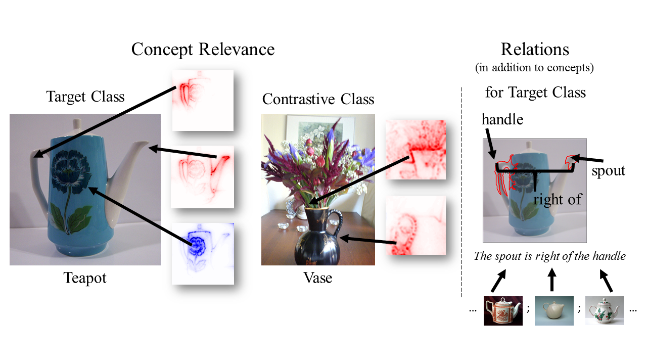
Figure 1: Explaining why a sample image belongs to the target class “teapot” by contrasting it with a sample from the contrastive class “vase” based on identified concepts (handle, spout) and their relations (“spout right of handle”)

In general, concepts are defined as mental representations for categories of objects Smith and Medin (2013). Concepts can be referred to with natural language, typically nouns. For instance, the objects in Figure 1 are referred to as ‘vase’ and as ‘teapot’. Natural categories such as different animals and also many human-made objects often have no crisp decision boundary Rosch (1973). Depending on the shape, and the presence of a handle or lid, an object might be identified as a teapot or not. Many concepts are members of a super-concept (a teapot belongs to crockery) and also have sub-concepts (e.g., Japanese teapots) Rosch (1973). Often, concepts can be characterized by the structure of their parts Simons (2000). For instance, a handle, a spout, and a lid are parts of a teapot.

In machine learning, concept learning is a special case of classification learning which approximates a binary target function that decides whether an instance belongs to a target class (concept) or not Mitchell (1997). In knowledge representation, ontologies are used to model domains of discourse by concept hierarchies Simons (2000). To derive such ontologies, concept analysis has been introduced Wille (2005). In general, the inclusion of domain knowledge can lead to more expressiveness and allows for more comprehensive evaluations of learned models. For example, knowledge about spatial relations can be used to perform reasoning on the structure of found concepts in images Renz (2002). In the spatial domain, reasoning on position, orientation, and distance are of particular interest (‘It is a teapot and not a vase because there is a handle right of a spout.’, see image on the right in Figure 1). Why considering concepts and relations at the same time? The separation of classes (here: “teapot” or “vase”) may be based on a common set of present concepts (e.g., handle, spout, flowers) and may therefore only be explainable if relevance of and spatial relations between those concepts are taken into account. Our approach extracts and localizes concepts for similar classes based on concept relevance representing the contribution of conjunct pixel groups to an image classification. Concepts positively contributing to a classification get positive relevance scores (red in Figure 1), negatively contributing concepts get negative scores (blue in Figure 1), whereas irrelevant concepts get a score near or equal zero (hwhite in Figure 1). Concepts can be labelled according to their appearance in images, where they have the highest absolute relevance score. We can learn from the above “teapot vs. vase” example that high relevance scores may correlate with similar concepts across classes (e.g., spout, handle) or that classes may differ by concept relevance (e.g., negative relevance for flowers on teapots). For our selected teapot example, we can explain the classification for the teapot by the relation “The example shows a teapot and not a vase, because the spout is right of the handle”, which holds, e.g., for all teapots oriented to the right in contrast to vases. Apparently, this finding does not hold for all teapots, but for a sub-group or cluster within the data.

For many real-world domains, objects are more or less typical members of their category Rosch (1973). Where categories are similar, it is more difficult to correctly classify objects near the category border McKee et al (2014). A vase with a bulbous body might be confused with a teapot; a teapot missing a handle might be confused with a vase. The same problem occurs in critical domains such as medicine. For instance, whether a tissue sample is indicative of a tumor class is harder to decide for borderline cases than for prototypical tissue patterns Bruckert et al (2020).

The application of XAI methods supports humans in comprehending how black box models such as CNNs derive a specific class output for a given input instance. This information can be used to examine the learned model. For instance, Clever Hans effects can be identified, that is, that the model output is right, but for the wrong reason, e.g., an image is classified as a horse, but based on copyright text or the background Lapuschkin et al (2019); Stammer et al (2021). Furthermore, learned models might be prone to make more classification errors near the decision boundaries between classes than near the center of the decision area. Several XAI methods have been proposed to support the exploration of decision boundaries of learned models. First, example-based explanations providing information about prototypes and critics have been suggested Kim et al (2016). Furthermore, contrastive explanations, where the neighborhood of a classified example in the instance space is explored have been shown to be highly efficient Teso and Kersting (2019); Miller (2021); Rabold et al (2022); Stammer et al (2021). Finally, cluster analysis, where clusters may be formed around very common or unusual or biased samples, has been demonstrated to be helpful Lapuschkin et al (2019). In general, contrastive explanations provide information about what has to be given or what has to be absent to make an object an instance of a specific concept. When used to explain a model to a human, contrastive examples uncover classification errors which might be corrected by providing new examples or constraints on the learning and prediction process to shift the decision boundary Teso and Kersting (2019); Dash et al (2022).

Attribution and backpropagation methods explain class predictions of a CNN (or other model types) by relating the class output to relevant features in the input. For image data, these features correspond to pixels or groups of pixels. Prediction boundaries are observed then on the prediction level, that is, evaluating whether a (contrastive) example is classified correctly or not. More recently, different approaches have been proposed to take into account information represented in intermediate convolutional layers of CNNs which will be discussed below Bau et al (2017); Fong and Vedaldi (2018); Rabold et al (2019); Achtibat et al (2022, 2023). Given information about concepts represented in intermediate layers of a CNN together with relations between such concepts allows us to provide more specific explanations, namely whether the prediction is based on the right concepts and relations or not. Representing both, concepts and relations in a human-understandable way further supports meaningful interaction with data, explanations, and the model itself.

Given that heatmaps cannot adequately explain the classification of a CNN model on complex, spatially-descriptive image data and that human-understandable explanations are needed that allow the decision boundary to be explored, we present a novel approach: the Concept- and relation-based explainer (CoReX). Our approach learns relations on top of concepts with the help of Inductive Logic Programming (ILP), which is inherently interpretable Muggleton et al (2018). CoReX makes the following contribution to the state of the art:

• It combines relevance-based concept extraction with interpretable relational learning to validate the predictive performance of a CNN w.r.t. contrastive classes that cannot be distinguished easily solely based on concepts, but rather general, domain-relevant spatial relations. Combining relevance information with ILP has already been researched Srinivasan et al (2019), but not for extracted concepts and not for intermediate layers of CNNs.

• For a collection of data sets (abstract, in-the-wild, scientific), we show quantitatively that our novel, combined explainer is faithful to a CNN model’s predictive outcomes. We further extend the quantitative evaluation of fidelity by a concept-based ablation study, that examines the performance of a CNN, when the CNN is permitted to use relevant and / or irrelevant concepts. We further qualitatively show that constraining relations in the learned interpretable relational model supports the identification and re-classification of incorrect or ambiguous image classifications. We provide a complete code basis to perform experiments presented here.

• In order to facilitate the exploration and adaptation of a CNN model’s decision boundary, we include contrastive explanations and relation-based cluster analysis into our approach.

Consequently, our main research question is, whether CoReX can identify concepts and relations from features learned by a CNN that are representative of contrastive classes and that are the main contributors to a model’s predictive performance. We further examine the explanatory capabilities of CoReX toward rectifiable models, in particular, its suitability for interactive learning by constraints with a human-in-the-loop.

The paper is organized as follows: In Section 2 we present works that are related to our approach. Section 3 introduces the technical background as a basis to the implementation of CoReX and defines important terminology. CoReX itself is described in Section 4. In Section 5 we introduce used materials and experimental settings in preparation of our evaluation, which is presented in Section 6, including quantitative and qualitative results. We conclude this article with future prospects in Section 7.

2 Related Work

Our approach to concept- and relation-based explanations relates to methods for disentangling representations in intermediate layers of CNNs. Furthermore, we focus on contrastive explanations which support identifying classification errors on decision boundaries. This type of explanation is especially relevant for explainable interactive approaches of machine learning (XIML).

2.1 Concepts, Relations, and Disentangled Representations

Research in human perception Miller and Johnson-Laird (2013) shows that the classification of an image depends not only on information about shape and texture but also on the constituents it is composed of and their relations. These constituents typically are concepts that can be named. Global explanations of categories typically rely on verbal or symbolic descriptions of their defining concepts and relations Du et al (2020). For instance, the concept of a grandparent can be explained as a person who is the parent of a parent Muggleton et al (2018); Rabold et al (2022) or the concept of a teapot could be explained as an item having a spout, a handle, and a lid where the lid is on top and the spout is on the side (see Figure  1). This observation that perception considers composition and relations has inspired approaches to disentangling representations.

One of the first approaches, NetDissect Bau et al (2017), considers a predefined pool of concepts given as objects, textures, and colors and finds units in convolution layers in a CNN whose activation maps are highly correlated with ground-truth masks of concepts in an image data set. The authors could confirm that representations at different layers disentangle different categories of meaning and that such disentanglements support interpretability of the representation learned by hidden units. Net2Vec Fong and Vedaldi (2018) is a modification of NetDissect, which learns a concept segmentation layer for locating concepts on images. The weight vector of this layer can then be understood as an embedding for the concept. Both methods rely on a predefined set of concepts and predefined masks which restricts explainability to the preconceptions of the model designers.

A recent method that builds upon the relevance-based approach LRP Lapuschkin (2019) is Concept Relevance Propagation CRP Achtibat et al (2022, 2023). CRP provides interpretable and class-specific features as concepts that are identified through class-conditioned decomposition of relevance maps instead of activation. In contrast to NetDissect and Net2Vec, CRP is able to automatically find sets of pixels that represent interpretable features in terms of concepts. Instead of comparing upscaled activation maps with ground-truth masks as in the previous approaches, CRP propagates class-specific relevance all the way to the input layer. We introduce the method in more detail in Section 4. A survey on other related concept-based explanation methods can be found in a recent survey by Poeta et al. Poeta et al (2023).

Approaches to relational symbolic learning, such as Inductive Logic Programming (ILP, Muggleton (1991)) explicitly learn conceptual structures. ILP-learned models are sets of rules for a target concept defined over sub-concepts and their relations. The set of rules constitutes a global explanation of a concept. Local explanations are generated when the model is evaluated for a specific instance Finzel (2024). The reasoning trace generated for the instantiated rule constitutes the explanation Finzel et al (2024). ILP has been applied as an explanatory surrogate model for image classification with CNNs Rabold et al (2020). Furthermore, approaches to generating contrastive explanations based on ILP models have been proposed Rabold et al (2022); Finzel et al (2024). An extensive survey on these and related methods can be found in Schwalbe and Finzel (2023).

2.2 Explanations for Interactive Learning

While measures of predictive accuracy give an overall indication of the quality of a learned model w.r.t. its performance on new inputs, explanations can provide a more specific understanding of the inner workings of a model. Global explanations reflect the general structure of a model. For relational data, ILP models constitute global explanations. ILP models can be learned stand-alone or in neuro-symbolic settings Manhaeve et al (2021). For relevance maps generated with LRP, Spectral Relevance Analysis (SpRAy) has been proposed Lapuschkin et al (2019) as an approach for global explanation generation. SpRAy applies spectral clustering on LRP explanations and thereby identifies different decision behaviors of the learned model. Prototypes are another form of global explanations which highlight the typical pattern of examples which are classified as belonging to a specific class Kim et al (2016).

While global explanations help to understand the general structure of the model, local explanations allow for understanding the class decision of a model for a specific instance. Heatmaps are an instance of local explanations in the form of visualizations on input images. Contrastive explanations can be given globally – by aligning two prototypes Artelt and Hammer (2021); Miller (2021) – or locally, by contrasting the current instance with one which is similar but belonging to a different class Herchenbach et al (2022); Rabold et al (2022); Finzel et al (2024). Contrastive explanations have been identified as especially helpful to understand the underlying reasons of classification errors. Therefore, they are helpful as guidance for interactive approaches to machine learning. Explanatory Interactive Machine Learning (XIML) has been introduced as a term for approaches that combine explanation generation and interactive model correction based on such explanations Teso and Kersting (2019). Corrections are given by revising not only erroneous class decisions (i.e., labels) but also the explanations, thereby constraining model adaption Teso et al (2022); Schramowski et al (2020).

3 Background and Terminology

This section introduces the theoretical background of methods integral to our approach as well as the basic terminology relevant to this work.

3.1 Extracting Visual Features with CRP

The basis to CRP Achtibat et al (2022, 2023) is LRP Lapuschkin (2019); Montavon et al (2019). LRP can be used to compute the contribution of individual pixels to a predictive outcome (relevance maps visualized as heatmaps). This is achieved by decomposing the relevance that is aggregated in an output neuron through a backward pass. We shortly introduce its basic computational rule:

$$R_{i}^{(l)}=\sum_{j}\frac{a_{i}w_{ij}}{\Sigma_{i}a_{i}w_{ij}}R_{j}^{(l+1)}$$ (1)

The relevance of a neuron $i$ in a layer $l$ can be determined as follows. Given the relevance $R_{j}$ of a neuron $j$ in a higher layer $(l+1)$ (e.g., the output neuron), the backward relevance flow from $j$ to $i$ is derived from dividing the product of the activation $a_{i}$ and the weight $w_{ij}$ by the sum of all activation weight products. If there is more than one neuron in $l+1$, the ratios get summed up by the outer sum $\sum_{j}$. Applying this rule in a complete backward pass leads to assigning relevance to every pixel $p$ of the input image. This score is computed in a conservative manner, meaning that $\sum_{p}R_{p}=f(x)$ holds for a classifier $f(x)$ on input $x$. The rule presented in Equation 1 has variants for different layers Montavon et al (2019). Selecting the best variant for the given CNN architecture is crucial to the quality of relevance computation. Here, we apply the $\epsilon$-variant, which was developed for intermediate layers in CNNs. These layers are usually convolutional layers. Thus, the rule works well for our approach as we only consider relevance in the last convolutional layer. The benefit of the $\epsilon$ rule is, that it preserves the most salient relevance and reduces noise resulting from weight sharing in convolutions Montavon et al (2019).

The relevance values of all pixels of an input constitute a relevance map. The CRP method we use to extract concepts is based on the assumption that a relevance map does not describe just one individual concept. Various filters contribute to the relevance that is distributed across pixels in an image Achtibat et al (2023). The advantage of CRP over LRP is that it can compute a class-conditional relevance map $R(x\mid y)$ for input $x$ w.r.t. a class $y$ and concept-conditional relevance maps by masking (intermediate) network outputs before applying LRP. It extends LRP as noted in Equation 1:

$$R_{i}^{(l)}(x\mid\theta\cup\theta_{l})=\frac{a_{i}w_{ij}}{\sum_{i}{a_{i}w_{ij}}}*\delta_{jc_{l}}*R_{j}^{l+1}(x\mid\theta)$$ (2)

Conditioning the relevance is achieved by setting all but the desired layer outputs to zero by multiplying a model output $f_{j}(x)$ with a Kronecker-Delta $\delta_{jy}$, such that $R_{j}^{L}(x\mid y)=\delta_{jy}f_{j}^{L}(x)$, where $L$ denotes an output layer. Here, $j$ is a convolutional layer represented by a tensor $(p,q,j)$, where $p,q$ denote the first and the second spatial axis of the tensor and $j$ the concept-axis, i.e., the filter. Conditioning the relevance by $\theta$ is possible for an individual network output for one or more filters in a convolutional layer. Achtibat et al. further assume that each filter encodes one particular concept throughout all model applications since their weights stay the same Achtibat et al (2022, 2023). This is the basis for ”filtering” specific concepts that were learned by the model.

The impact of a single concept $c$ on the prediction outcome of $x$ is represented by the sum of relevance in the respective layer (see Equation 3). It helps to select the concepts contributing most to a prediction. Achtibat et al. use Relevance Maximization (RelMAx) to find for every concept a set of input samples (reference samples), where the concept contributed most to the prediction (see Equation 4).

$$R^{l}(x\mid\theta_{l})=\sum_{i}R_{i}^{l}(x\mid\theta_{c})$$ (3)

$$\tau_{max}^{rel}(x)=\max_{i}R_{i}(x\mid\theta).$$ (4)

By using a concept-specific constraint $\theta$ on RelMax, a set of reference samples from the target class is selected. For this set, a human expert can decide upon the overall concept label for the filtered pixel regions in reference samples. We integrated this component into our implementation in order to optionally support labeling of concepts by human users (e.g., a teapot handle). Localization of a concept within a reference image is done by extracting the receptive field information Achtibat et al (2022, 2023). The rest of the image is then masked out to emphasize on the region of interest, where the concept displays. As this work focuses on the technical evaluation of our proposed approach, we did not integrate the reference sampling into our experiments, however, we used it for validity checks on identified concepts. Furthermore, reference sampling helps to label concepts more efficiently. Presenting reference samples to a (human) labeler according to the relevance rank of a concept helps to prioritize which concepts should be labeled first. In Section 4, we will explain how we take advantage of concept ranking to learn an interpretable relational surrogate model on fewer data, yet faithful to a CNN model’s predictions.

In advance to describing how we learn a surrogate model on top of extracted concepts and their relations, it is worth mentioning that CRP assigns concepts with positive or negative relevance, depending on whether they contribute to a decision in favor of the target class or not (likewise to LRP Lapuschkin (2019)). A relevance value equal or near zero defines a low or missing contribution in any direction. To be able to interpret the explanations produced by our approach, we define the meaning of relevance such that if the relevance of some concept $c$ is positive, this concept is located in the image region for desirable reasons. If the relevance of some concept (not necessarily the same $c$) is negative, the concept should not be there, whichever concept is located at the relevant pixel area instead of the desired one. We want to point out that images cannot contain nothing. If a concept of interest is not displayed, there always will be another concept, pixel group or pixel value with possibly no defined meaning instead.

3.2 Learning Symbolic Hypotheses with ILP

ILP is a machine learning approach that allows for induction and deduction. It has been introduced back in the year 1991 by Stephen Muggleton Muggleton (1991). Learned models are logic programs, which are induced from examples. These logic programs can then be executed to derive explanations for classifications. The overall goal of ILP is to derive a hypothesis $H$, also called theory, from a set of examples $E^{+}$ belonging to the target class and a set of examples $E^{-}$ not belonging to the target class and background knowledge $B$. The background knowledge $B$ holds features of examples and optionally reasoning rules (called domain theory) to derive further properties, e.g., transitive relations. $H$ is induced such that $\forall e\in E^{+}:B\cup H\models e$ and $\forall e\in E^{-}:B\cup H\not\models e$. The first condition demands $H$ to be complete, i.e., covering all positive examples $E^{+}$. The second condition demands it to be consistent, i.e., not covering negative examples $E^{-}$.

These formal properties make ILP susceptible to noise in the underlying data. This apparent downside comes in favor for generating explanations for flawed models since ILP will not be robust to examples incorrectly labeled by some base model, the explanandum. When instances contain noisy concepts or relations which the model deems to be important, hypotheses generated by ILP can make the noise explicit to the user which in turn gives them the power to evaluate the model as well as the data.

For theory induction, this work uses the Prolog-based ILP Framework Aleph Srinivasan (2007). The basic procedure that is performed by Aleph follows four steps. First, for as long as there is an example in $E^{+}$, a candidate example $e\in E^{+}$ gets selected. In the second step, a most specific clause (so-called bottom clause) is constructed, which entails the selected example and adheres to $B$. Then, Aleph searches for a rule that is more general than the bottom clause, i.e., a subset of all literals in the current clause. Aleph tests which examples from $E^{+}$ or $E^{-}$ are covered by the rule and finally removes all (now redundant) examples from the list of candidate examples, that are already covered. This procedure is repeated until all examples are covered, either by a rule or added to the theory as instances without generalization Srinivasan (2007).

4 Method

Our approach is illustrated in Figure 2. It combines (1) extracting concepts from visual features learned by CNNs with CRP, and (2) learning symbolic hypotheses by means of relations with ILP, where we integrate spatial relational knowledge for a more expressive evaluation of the CNN output. The visual and verbal explanations resulting from (1) and (2) are the basis for providing (3) contrastive explanations, and (4) rule-based cluster analysis for a given explanandum. To evaluate the importance of the concepts and relations that are learned by the surrogate ILP model, we then suppress concepts in learned CNN models by (5) masking the respective concepts before application on the same data, and we suppress relations by (6) constraining relations in the ILP model to identify and re-classify samples based on human domain-knowledge.

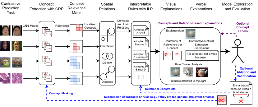
Figure 2: Overview of our CoReX approach for explaining and evaluating CNN image classifications with concept- and relation-based explanations and constraints (concept masking and relational constraints)

4.1 Building Background Knowledge from Concepts

In Section 3 we introduced how concepts are extracted from the relevance of filters in convolutional layers of CNN models. In principle, we only analyze the last convolutional layer of our utilized models for concept extraction. More details on the architectures of our models and their parameters are given in Section 5. For the preparation of learning a surrogate model with ILP, we store concepts in the background knowledge $B$ as introduced earlier. That means, we write a first-order-logic 2-ary predicate to the Prolog background knowledge for each example image if a concept is present (see first line of part D in Figure 3).

Depending on the architecture of the respective CNN model, the amount of extracted concepts can be large ($>$ 500) as noted in Section B of the appendix. One observation we make is that the majority of these concepts often has low relevance values. This does not necessarily imply that these concepts are useless, however, it is probable that many of them can be removed without seriously harming the performance of a CNN model. For improved computational performance, we therefore decided to write only the concepts to the background knowledge that have a relevance, which exceeds a predefined relevance threshold. Since every model may produce a different distribution of relevance dependent on the data set under consideration, we set the threshold according to a quantile of the relevance distribution. This can result in varying amounts of concepts in the background knowledge accross data sets, however, this strategy is more flexible and less biased compared to a fixed amount of concepts or a fixed value for a threshold.

In our experimental results in Section 6, we speak of three different kinds of concepts. Based on the thresholding, we distinguish between relevant concepts (in the background knowledge) and irrelevant concepts (not in the background knowledge). Within the concepts that are in the background knowledge, we further introduce another category of concepts: the concepts from the background knowledge that are included in the rules of the interpretable surrogate model after learning a theory with ILP.

Besides storing predicates for concepts that exceed the relevance threshold, we also compute spatial relations between these concepts.

4.2 Integration of Spatial Relational Knowledge

The Prolog background knowledge that basically consists of concepts with positive or negative relevance, can be additionally enriched by knowledge that is generally applicable to the image data domain, such as spatial relations. The relations are labeled according to existing spatial frameworks. In particular, we integrate a symbolic representation of relations from the DE-9 Intersection Model Clementini and Felice (1996), orientation in a 8-cell grid and categorized distance. For each framework, we first localize the pre-computed concepts with the help of concept relevance, we then transform the conjunct pixel regions into polygons and relate the polygons in accordance to the respective spatial framework. We then store the labeled relations in Prolog syntax as 3-ary predicates with 2-ary predicates as arguments for denoting the relevance sign of a concept (see bottom lines of part D in Figure 3). An overview of all possible predicates is presented in Section A of the appendix.

4.3 Model Truth and Explainer Truth

A useful interpretable surrogate model should produce outcomes similar to the machine learning model in question as a precondition to providing explanations faithfully. In particular, observing the output of the base model and the output of the interpretable explainer gives insight in how closely an explainer resembles the model’s predictive behavior. To compare the two, we use the terms model truth $\hat{y}_{d}$ and explainer truth $\overset{e}{y}_{d}$ for a given sample $d$. These terms manifest what the model or the explainer deem to be true for $d$. Both of these give either 1 or 0 depending on whether $d$ was being rendered as belonging to a target class or not. We use this notation and terminology for evaluating the fidelity of an explainer (see Subsection 5.3).

Having introduced concept extraction, rule induction on concepts, spatial relations between them and evaluation terminology, we put all components together that form our approach and introduce its algorithmic foundation in the next section.

4.4 Algorithm

We summarize the main procedure of CoReX as presented in Algorithm 1. For all positive and negative model truth examples, background knowledge $B$ for ILP is generated. For one example $e$, concept relevance maps $C_{l}$ are found by CRP on all selected layers $l\in L$. The most important concepts exceeding the relevance threshold $\tau$ are used to localize polygons $P_{e}$ fitted on the relevance maps. Utilizing spatial calculi, relations between the polygons are then found and stored in symbolic form. This information is then used to induce a logic theory $H$ in form of rules by Aleph. Optionally, it is possible to provide the CRP procedure with a parameter $\varphi$ for masking concepts. Furthermore, in ILP it is possible to add a set of constraints $\phi$ on concepts and relations that must not appear in learned theories.

Algorithm 1 CoReX Algorithm

Input: Original model $f$, positive/negative model truth samples $E^{+}$/$E^{-}$, set of probed layers $L$, optional masking $\varphi$, relevance threshold $\tau$, set of possible relations $S$, optional ILP constraints $\phi$

1:$B\leftarrow\text{domain theory}$

2:for all $\odot\in\{+,-\}$ do

3:     for all $e\in E^{\odot}$ do

4:         $P_{e}\leftarrow\emptyset$

5:         for all $l\in L$ do

6:              $C_{l}\leftarrow\text{crp}(e,f,l,\varphi)$

7:              $C^{*}_{l}\leftarrow\text{filter\_concepts}(e,l,q)$

8:              for all $c\in C^{*}_{l}$ do

9:                  $P_{e}\leftarrow P_{e}\cup\text{localize}(c,\tau)$

10:              end for

11:         end for

12:         $R_{e}\leftarrow\text{find\_relations}(P_{e},S)$

13:         $B\leftarrow B\cup R_{e}$

14:     end for

15:end for

16:$H\leftarrow\text{induce}(E^{+},E^{-},B,\phi)$

17:return H

An exemplary rule for our running example of separating teapots from vases is presented below. It expresses that some sample A belongs to the target class (here: teapot) if there are two concepts in A (concept “spout” and concept “handle”), both concepts contributing with positive relevance (“pos”), and it holds that the “spout is located right of the handle” (as presented in Figure 1).

    is_class(A) :-
        right_of(A, pos(A, spout), pos(A, handle)).
    

The rule results from the process presented in Figure 3. For each $e\in E^{+}$ and $e\in E^{-}$ we get the classification of $e$ and the CRP-based concepts, conditioned by the target (see step A in Figure 3). We then localize and polygonize the extracted concepts (step B). Then, spatial relations between polygons are computed (step C) and the resulting relations are transferred into Prolog syntax as input to ILP (step D). A theory is induced (step E) and finally, evaluation analysis or explanations take place (steps in F). For explanations, the Prolog syntax is translated into natural language based on a fixed scheme.

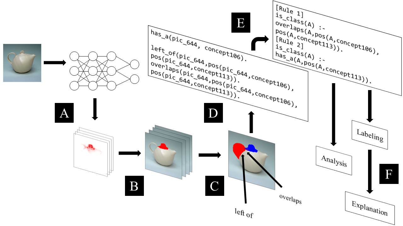
Figure 3: Overview of the process of generating explanations with ILP from extracted concepts and learned relations

5 Experiments

This section presents the materials, metrics and the experimental setting of our evaluation.

5.1 Models

For our experiments, we use two CNN architectures well established, especially for LRP-based explanation methods, namely VGG16 Simonyan and Zisserman (2015) and ResNet50 He et al (2016). For both architectures exist optimized variants of the $\epsilon$ rule for the computation of concept relevances Achtibat et al (2022, 2023), which is another favorable property of the chosen architectures.

For the classification of most of our selected data sets, we use VGG16 models pre-trained on the ImageNet database Deng et al (2009) and fine-tune the fully connected layers on our selected data sets. Table 1 states the performance metrics and hyperparameters we use for the fine-tuning on our selected data sets. This way, we preserve the features learned in the network, while updating the weights. The rationale behind not fine-tuning features for our specific classification tasks is that we assume that the pre-trained features are already general purpose for a variety of tasks. By fine-tuning the fully connected layers, the relevance values for CRP, which is calculated down-stream dependent on weights, become task-specific and thus indicate relevance of features for a specific classification problem. One particular data set (see descriptions below) is classified based on a pre-trained model with a ResNet50 architecture. For this network, we fine-tuned the last layers, in particular the average pooling layer and the linear output layer. This was necessary, since we had to make adaptations to the composition of classes. More details are given in the paragraphs on the chosen data sets.

Table 1: The characteristics of the non-contrastive pre-trained models used for contrastive classification after fine-tuning (CE is cross entropy; BCE is its binary equivalent)

	#Train	#Test	Train F1	Test F1	#Class	Batch Size	Max. Epochs	Optimizer	Loss Function	Learning Rate
Picasso (VGG16)	18,002	1998	0.9933	0.9924	1	32	20	Adam	BCE	0.0001
Adience (VGG16)	9942	2252	0.9913	0.8702	2	32	20	Adam	CE	0.0001
Teapot and Vase (VGG16)	231	100	1.0000	0.9200	2	32	20	Adam	CE	0.0001
PathMNIST (ResNet50)	25,765	2462	0.9974	0.9709	2	128	10	Adam	CE	0.001

For all our models, we only examine features in the very last convolution layer of the architecture, although the CRP method would allow for inspection of preceding layers as well. This is of particular interest, when concepts may be organized in a hierarchy. This would, however, require the consideration of the relevance flow between different layers, for which there exists no thoroughly evaluated method for CNNs so far.

5.2 Data Sets

The data sets we have chosen cover a range of characteristics, which makes them suitable for a comprehensive evaluation of our approach. We use artificially generated image data, benchmark image data, showing either static and aligned objects or in-the-wild recorded scenes, and a benchmark that contains scientifically and application relevant samples, e.g., for medical diagnosis. All data sets are thoroughly chosen w.r.t. the criterion that they contain classes, which are very likely to share concepts, while not sharing the same spatial relationships between those concepts. Figure 4 shows example images from the data sets.

(a) Picasso: correct (left) vs incorrect (right) faces

(b) Adience: female (left) vs male (right)

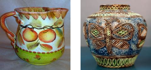
(c) ImageNet: teapots (left) vs vases (right)

(d) PathMNIST: cancerous (left) vs healthy (right) tissue

Figure 4: Examples of contrastive classes

Picasso: Correct Faces versus Incorrect Faces.

The Picasso data set Rabold et al (2020) is a constructed data set derived from the FASSEG set Khan et al (2015) for segmentation of facial features in frontal faces. Picasso contains 224x224 images where the positive class holds faces with three features, the eyes, nose and mouth, in natural position, whereas in the negative class, the features are swapped randomly. For ILP, we use 250 each from train and test data. The reason, why we evaluate our approach on training data and test data is that explanations may differ depending on the kind of data. Explanations on training data evaluate which representations the model has learned, while explanations on test data evaluate how well these explanations generalize.

Adience: Female versus Male Persons.

The Adience data set Eidinger et al (2014) features 224x224 cropped face images labeled by gender. The images were taken in the wild and contain a variety of backgrounds and illumination conditions. We sampled 200 male and 200 female labeled images. We chose the data set as we expected different spatial relations for (probably biased) properties of persons, like the localization of hair due to its length.

ImageNet: Teapots versus Vases.

We took 161 images from teapots and 170 images from vases (224x224) from the ImageNet data set Deng et al (2009). Because labels were missing, we let the original VGG16 classify these images. The same images were taken as input to generate our explanations. Due to the small size of the data set, we could only use training data as well as test data for the VGG16 evaluation. For our ILP model, we only considered training data for evaluation.

PathMNIST: Healthy versus Tumorous Tissue.

The PathMNIST data set Kather et al (2019), subset of MedMNIST Yang et al (2021), consists of 28x28 pathological histology slides taken from healthy as well as cancerous colon tissue. PathMNIST originally is a 9 class classification task. For our experiments, we re-sampled the images to form a 2-class task by keeping all images in the cancer-associated class as positive images (12,885) and then performed a stratified sampling over the other 8 healthy classes to receive approximately as many images (12,880) in the contrastive class. We sampled 250 positive and 246 negative images for ILP.

5.3 Evaluation Metrics

When evaluating the generalization power of our models, we use the standard F1 metric (harmonic mean of precision and recall). The respective scores for the ground truth labels of the train and test sets can be found in Table 1.

For the evaluation of fidelity of an explanation model w.r.t. an original black box model, we compare the model truth (output of the original model) with the explainer truth (output of the explanation model) which were introduced in Subsection 4.3. Adopting the method from Rabold et al (2020), in accordance with the notion of fidelity introduced in Guidotti et al (2019) and Carvalho et al (2019), we calculate the accuracy of the explainer truth $\overset{e}{y}_{d}$ w.r.t. the model truth $\hat{y}_{d}$ when feeding instances $d$ from a data set $D$, where $\delta(a,b)$ is 1, if a and b are equal and 0 otherwise (Equation 5). For better readability, the index of the samples is omitted.

$$\frac{\sum_{d\in D}\delta(\hat{y}_{d},\overset{e}{y}_{d})}{|D|}$$ (5)

5.4 Ablation Study

We combine model explanations with ablation studies to evaluate the used CNN models (see section 6.1 for more details). In machine learning, ablation studies refer to the removal of architectural components or model features. The goal is to evaluate a model w.r.t. its predictive performance and the contribution of architectural components or features to the predictive outcome. Approaches for CNN ablation are, e.g., pruning, drop out or suppression of activation and weight flows between neurons Choi et al (2022).

To perform an ablation study based on our concept- and relation-based explainer CoReX, we apply masking on the filters of the CNN to suppress concepts. This technique is realized in a first step by setting all filters in the CNN to zero that do not match with concepts appearing in the background knowledge of ILP (masking irrelevant concepts). We measure the predictive performance of the adapted CNN. We then mask all irrelevant concepts as well as the concepts that appear in a theory learned by ILP (masking rule concepts). We hypothesize that, if the performance drop is larger for the second case compared to the first one, the concepts learned by the CNN and provided to ILP have an decreasing effect on the confidence of the CNN in accordance to their relevance. For our experiments we applied Aleph with default settings.

For a qualitative evaluation of our approach, we integrated user-defined constraints on relations and concepts as provided by the Aleph framework Srinivasan (2007). In Section 6 we demonstrate the usefulness of such constraints in combination with contrastive and clustered rule-based explanations.

6 Evaluation

This section presents the main results of our experiments, including an analysis of the fidelity of our interpretable, relational surrogate model as well as the predictive performance of both, the base model as well as the surrogate model, respectively. We further examine the explanatory applicability of CoReX, in particular for contrastive explanations and cluster analysis. We further discuss the role of constraints in our approach, which extends beyond the masking and constraining in our ablation study.

6.1 Fidelity and Predictive Performance

Table 2 presents the correct and incorrect predictions for all CNN models on training and test data, which form the input for the ILP-based explainer. The table denotes the amount of positive examples ($E^{+}$) and negative examples ($E^{-}$), accordingly. The column “# Rule Concepts” documents the amount of concepts that were included by ILP into rules.

Our results indicate that our explanations (generated for the samples stated in Section 5.2) have a high fidelity w.r.t. the original model when measured by the comparison of the model truth and the explainer truth (as calculated by the fidelity Equation 5). Table 3 then states the fidelity of the ILP explanations for the training and test samples.

We additionally measured the F1 scores for models that were altered by masking. We differentiate two cases: (1) masking concepts that occurred in the learned ILP theory as well as irrelevant concepts versus (2) masking only concepts deemed irrelevant because they are not occurring in the ILP background knowledge. We expect to see a drop in performance when masking concepts occurring in rules. Table 3 shows that in almost all scenarios, the performance is reduced (in bold: F1 score of “Rule + Non-BK-Masking” is lower than the F1 score of “Non-BK-Masking”). This further may be an indicator that the learned rules constitute explanations of the original model’s prediction strategies. The magnitude of the performance drop appears to be rather low, however, related to the amount of masked concepts and the amount of concepts in total (see Section B) this drop is not insignificant. Thus, we can observe that the concepts from the background knowledge, which have a high relevance due to the relevance threshold, but are not included in ILP rules cannot fully compensate for the impact of the concepts in learned rules. This may not hold for the Teapot and Vase experiments on the training set as well as the PathMNIST test set, since the performance is equal in both of the masking settings. Thus, the results do not perfectly support our hypothesis of dropping performance upon masking concepts from learned rules, however, they highly support it. Moreover, there was not a single case in which the performance of the network improved when concepts were masked. We further examined at which rank in the relevance ranking the concepts from rules with the largest coverage appeared across all samples. The frequency of occurrence per rank is indicated in Section D. We can see that the top 10 most frequent ranks per concept are usually the first ranks or at least upper 20 % top ranks of possible ranks. In few cases, higher rank numbers occur in the 10 most frequent ranks. This can be explained by auxiliary concepts that occur as part of a relation together with more important concepts, indicating that not only single concept occurrences are important but also the inter-relations between them. In summary, the findings support the claim that not only the calculated relevance can be transferred to the importance of concepts, but also the spatial constellation of concepts as learned by the ILP model contributes to the performance of an image classifier.

Table 2: Model truth for the train/test data (seen/not yet seen by the model) and the number of concepts occurring in the learned rules

Experiment	True Positives	True Negatives	False Positives	False Negatives	#Rule Concepts	ILP Input ($E^{+}$)	ILP Input ($E^{-}$)
Picasso-Train (VGG16)	250	243	7	0	44	257	243
Adience-Train-FM (VGG16)	197	195	5	3	10	202	198
Adience-Train-MF (VGG16)	195	197	3	5	9	198	202
Teapot-Vase-Train (VGG16)	157	166	4	4	10	161	170
Vase-Teapot-Train (VGG16)	166	157	4	4	13	170	161
PathMNIST-Train (ResNet50)	250	246	0	0	6	250	246
Picasso-Test (VGG16)	250	250	0	0	31	250	250
Adience-Test-FM (VGG16)	179	164	36	21	10	215	185
Adience-Test-MF (VGG16)	164	179	21	36	6	185	215
PathMNIST-Test (ResNet50)	238	239	7	12	7	245	251

Table 3: Explainer fidelity and train/test data metrics for the networks after masking of rule + non-background-knowledge (BK) concepts compared to only masking non-background-knowledge concepts. Bold values indicate an expected drop in performance

		Rule + Non-BK-Masking		Non-BK-Masking
Experiment	Explainer Fidelity	Amount of Masked Concepts	F1 score	Amount of Masked Concepts	F1 score
Picasso-Train (VGG16)	0.9860	208	0.2985	164	0.9921
Adience-Train-FM (VGG16)	1.0000	18	0.9437	8	0.9913
Adience-Train-MF (VGG16)	1.0000	17	0.9896	8	0.9913
Teapot-Vase-Train (VGG16)	0.9970	24	1.0000	14	1.0000
Vase-Teapot-Train (VGG16)	0.9970	27	1.0000	14	1.0000
PathMNIST-Train (ResNet50)	1.0000	1384	0.9872	1378	0.9873
Picasso-Test (VGG16)	0.9980	193	0.6689	162	0.9924
Adience-Test-FM (VGG16)	0.9975	15	0.8079	5	0.8708
Adience-Test-MF (VGG16)	0.9975	11	0.8673	5	0.8708
PathMNIST-Test (ResNet50)	0.9980	1374	0.9367	1367	0.9367

6.2 Explanatory Applicability of CoReX

6.2.1 Contrastive Explanations and Clusters

We enhance CoReX by exploration of sample classifications based on contrastive explanations and rule-based cluster analysis. Contrastive local explanations are produced by evaluating our ILP model for a specific misclassified sample. This means that we try to unify the background knowledge of a misclassified sample with rules from the ILP model (e.g., the rule with the highest coverage). The evaluation returns concepts and relations that are missing in the sample in order to belong to the target class. CoReX provides a component that verbalizes these failures with the help of an implemented Prolog-based prover (see code repository given in Section Declarations). Note that concepts presented here, have been labeled according to a majority vote for a label derived from the reference sampling with maximized relevance, introduced in Section 3.

Rule-based cluster analysis allows for outlier and prototypical example detection. In particular, we analyze, which rules jointly cover which samples by building the power set of combinations. We examine clusters that cover most of examples, samples not covered by any rule, and clusters that cover few samples with just a small set of rules. The clusters computed for the different data sets can be found in Section C of the appendix.

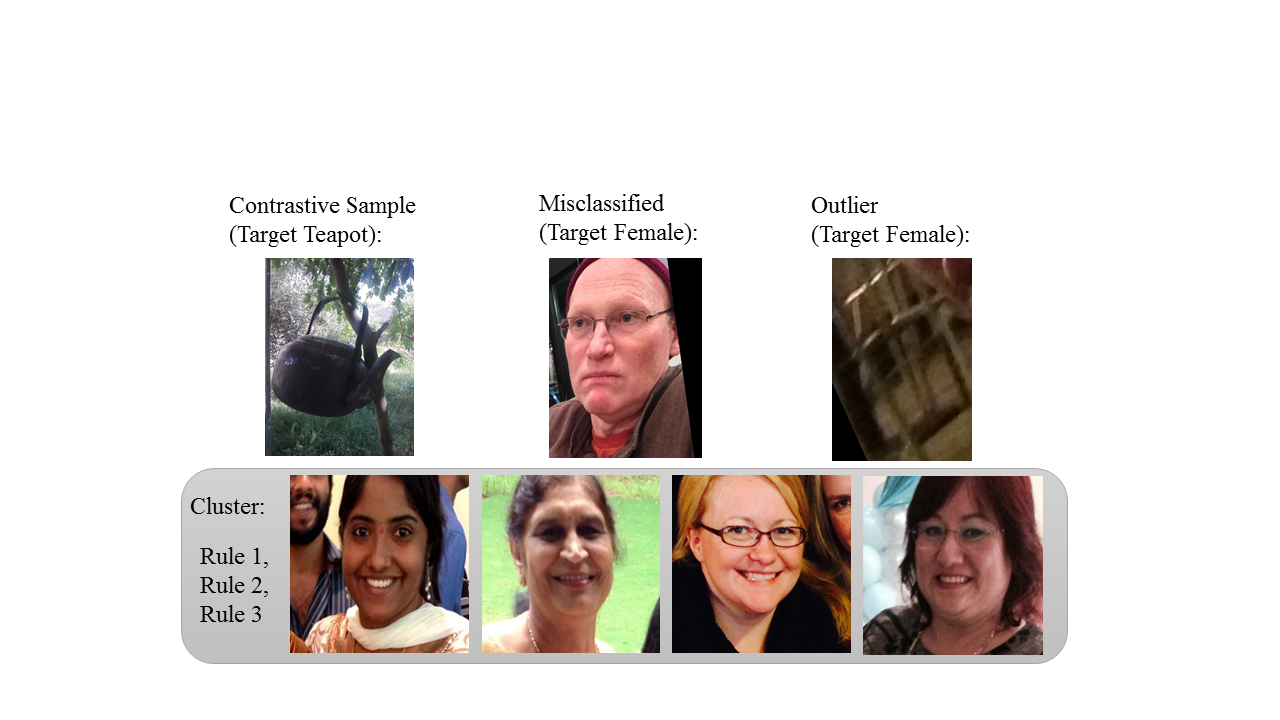
Figure 5: Teapot (top left), false positive female (top middle), outlier female (top right) and rule cluster for smiling persons (bottom row)

In Figure 5 we present a collection of interesting cases. Consider the contrastive sample from ImageNet (target: teapot), which is a teapot in the ground truth as well as in the model truth (CNN), but not in the explainer truth (ILP). When evaluating the ILP model on the sample, we can observe that a concept from the best covering rule was missing in the background knowledge: the spout. It did not belong to the most relevant concepts for this sample and was therefore not included in the background knowledge. Probably, the tree in the image may have been the disturbing factor.

Our cluster analysis on the Adience Test data set (target: female) yields interesting results as well. The most representative cluster mainly contains samples with the relation “eyes above of smiling mouth” (see Figure 5). Further analysis identifies a cluster that is small with few examples covered. In this cluster all samples have in common that one concept comprises a border artefact, among others this applies to the outlier, which is displayed in the top row on the right side of Figure 5. One cluster was empty (an example not covered by any rule. This example was misclassified by the CNN model as “female”, although its ground truth was “male”. The coverage of the sample fails due to failed unification of the background knowledge of the sample with the learned rules.

7 Conclusion and Future Work

We presented CoReX as a novel XAI approach for image classification with CNNs, which relies on identifying concepts and relations between concepts in intermediate layers of a CNN. Concept relevance ist combined logic rules constructed from learned ILP theories. An evaluation with different data sets shows that the CoReX explainer is highly faithful to the examined CNN models and that it provides meaningful explanations for correctly and incorrectly classified instances. In the next step, a human could interact with the model as demonstrated in the evaluation of our approach, giving the information about what concept must be suppressed or kept by a model or explainer, pathing the way for regularization of the model to align with the provided corrective feedback Bontempelli et al (2023); Dash et al (2022). The evaluation of our approach and similar future approaches would highly benefit from a larger availability of contrastive data sets, where the classification of an image depends on the relations between concepts. As already laid out in the motivation, the instances of many domains in the real world can be explained in a way that aids humans by contrasting them with similar instances. We argue that there is a need for more data sets, that help researchers to explore methods and to generate expressive, contrastive and potentially multimodal explanations for improved explainability.

Declarations

7.1 Funding

This work was partially funded by the German Federal Ministry of Education and Research under grant FKZ 01IS18056 B, BMBF ML-3 (TraMeExCo, 2018-2021) and partially supported by the German Research Foundation under grant DFG 405630557 (PainFaceReader, 2021-2023).

7.2 Ethics approval

Not applicable.

7.3 Consent to participate

Not applicable.

7.4 Consent for publication

The authors affirm that human research participants provided informed consent for publication of the images in Figures 4, 5 and LABEL:fig:rectifiable. In particular, the Adience data set Eidinger et al (2014), consists only of material, including human faces, which has been deliberately provided under a Creative Commons (CC) licence on Flickr. The Picasso data set Rabold et al (2020) contains completely retouched faces. Moreover, facial features (eyes, nose, mouth) are randomly taken from a pool of features to generate artificial faces, which render persons unrecognizable.

7.5 Competing interests

The authors have no conflicts of interest to declare that are relevant to the content of this article.

7.6 Availability of data and materials

See code availability.

7.7 Code availability

The code basis of our CoReX approach and scripts for evaluation purposes are available at the linked repository.

7.8 Authors’ contributions

All authors contributed to this work. B.F. initiated the paper, wrote a first complete draft and contributed to all sections for the submitted version. B.F. and P.H. developed the concept behind the methodology. P.H. contributed to the implementation of the methodology. B.F. revised and extended the implementation. P.H., J.R. and B.F. planned and carried out the experimental evaluations and revised the first draft. J.R. provided substantial input for related work on concept analysis and fidelity measures. U.S. contributed with revisions of the first draft and substantial input for related work on cognitive concepts. All authors have read and approved the submitted version of this paper.

7.9 Acknowledgments

We would like to thank Reduan Achtibat who provided support for the configuration of Concept Relevance Propagation and Sebastian Lapuschkin for fruitful discussions on relevance-based feature extraction.

Appendix A Spatial Relations

See Table 4.

Table 4: Overview of all supported relations. Relations are organized in unary and binary sets and apply w.r.t. a sample. Negative relations represent a concept’s relevance scores sign. Sets like the SimpleAlignment, Distance and Surrounding are implemented based on the geometric interfaces of the python shapely library Gillies (2022). CompassAlignment is loosely based on a direction-based spatial navigation model of Sriharee (2015). NineIntersectionModel is based on the DE-9IM developed by Clementini, et al. Clementini and Felice (1996); Clementini et al (1993) with the omission of the intersect-relation

Set	relation	definition	semantic
unary relations
Existence	$has\_a(A)$	$neg(A)\lor pos(A)$	has A
Negativity	$neg(A)$	$R(A)<0$	A, that shouldn’t be there
	$pos(A)$	$R(A)>0$	A, that should be there
binary relations
SimpleAlignment	$above\_of(A,B)$	$A.centroid.y<B.centroid.y$	A is above of B
	$below\_of(A,B)$	$A.centroid.y>B.centroid.y$	A is below of B
	$left\_of(A,B)$	$A.centroid.x<B.centroid.x$	A is left of B
	$right\_of(A,B)$	$A.centroid.x>B.centroid.x$	A is right of B
CompassAlignment	$center(A,B)$	$A.centroid.buffer.intersects(B)$	B is centered on A
	$middle\_right(A,B)$	$\triangle(A,l_{\frac{15}{8}\pi},l_{\frac{1}{8}\pi}).intersects(B)$	B is middle right to A
	$bottom\_right(A,B)$	$\triangle(A,l_{\frac{1}{8}\pi},l_{\frac{3}{8}\pi}).intersects(B)$	B is bottom right to A
	$bottom\_middle(A,B)$	$\triangle(A,l_{\frac{3}{8}\pi},l_{\frac{5}{8}\pi}).intersects(B)$	B is middle bottom to A
	$bottom\_left(A,B)$	$\triangle(A,l_{\frac{5}{8}\pi},l_{\frac{7}{8}\pi}).intersects(B)$	B is bottom left to A
	$middle\_left(A,B)$	$\triangle(A,l_{\frac{7}{8}\pi},l_{\frac{9}{8}\pi}).intersects(B)$	B is middle left to A
	$top\_left(A,B)$	$\triangle(A,l_{\frac{9}{8}\pi},l_{\frac{11}{8}\pi}).intersects(B)$	B is top left to A
	$top\_middle(A,B)$	$\triangle(A,l_{\frac{11}{8}\pi},l_{\frac{13}{8}\pi}).intersects(B)$	B is middle top to A
	$top\_right(A,B)$	$\triangle(A,l_{\frac{13}{8}\pi},l_{\frac{15}{8}\pi}).intersects(B)$	B is top right to A
NineIntersectionModel	$disjoint(A,B)$	$A.disjoint(B)$	A is disjoint of B
	$equals(A,B)$	$A.equals(B)$	A equals B
	$touches(A,B)$	$A.touches(B)$	A touches B
	$overlaps(A,B)$	$A.overlaps(B)$	A overlaps B
	$covers(A,B)$	$A.covers(B)$	A covers B
	$contains(A,B)$	$A.contains(B)$	A contains B
	$covered\_by(A,B)$	$A.covered\_by(B)$	A is covered by B
	$within(A,B)$	$A.within(B)$	A is within B
Distance	$close\_to(A,B)$	$A.distance(B)<range$	A is close to B
special binary relation
Surrounding	$amid\_x(A,B)$	$B.between(A_{1}.centroid.x,A_{2}.centroid.x)$	B is horizontally
			surrounded by A
	$amid\_y(A,B)$	$B.between(A_{1}.centroid.y,A_{2}.centroid.y)$	B is vertically
			surrounded by A

Appendix B Number of concepts

Figure 6 shows the distribution of concepts for all experiments, split by the concepts occurring in the rules of a learned ILP theory, the other concepts in the background knowledge, and the irrelevant concepts. Table 5 additionally gives the absolute values.

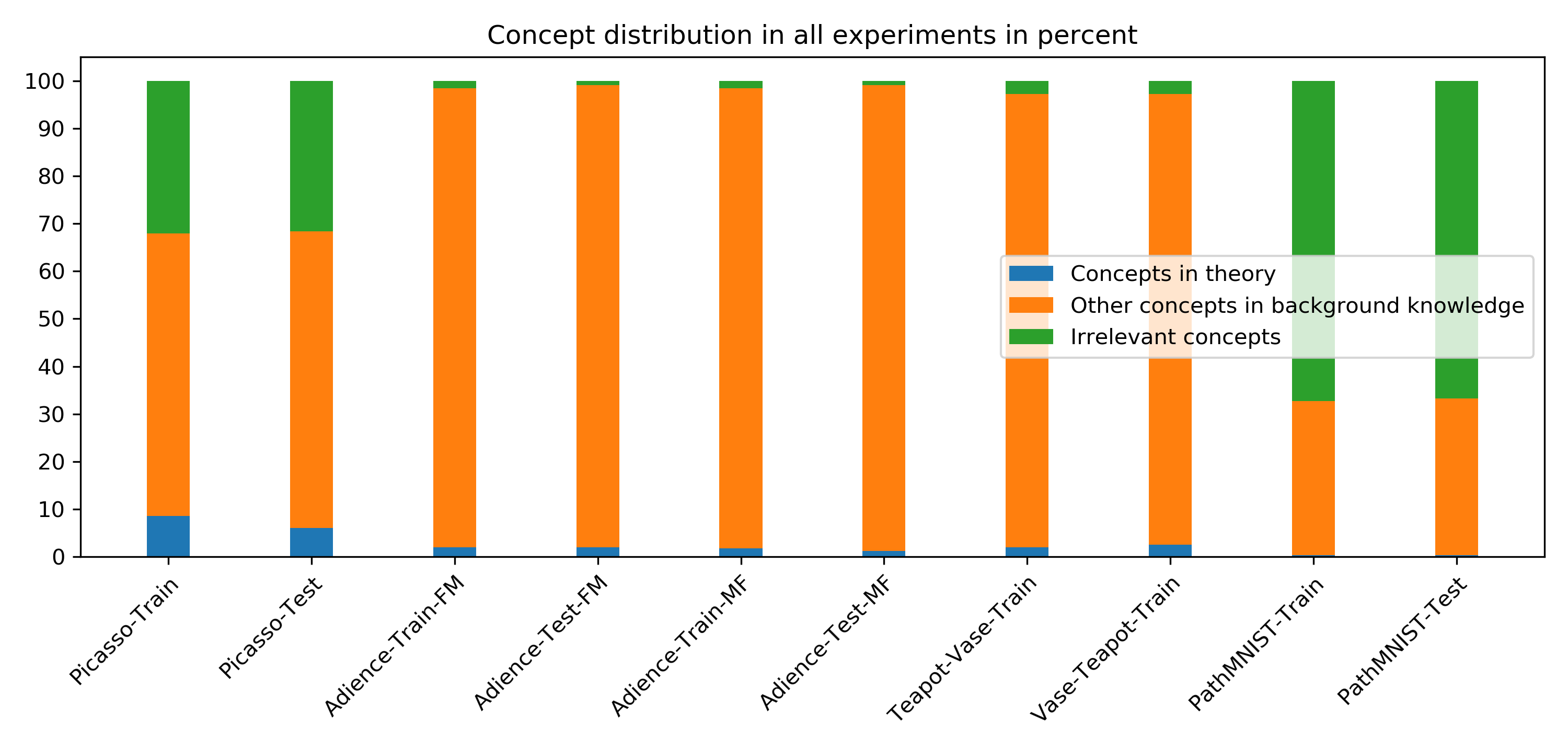
Figure 6: The distribution of concepts (given in percent) in the theory, in the background knowledge (excluding the theory concepts), and irrelevant concepts. See Table 5 for a detailed breakdown

Table 5: The number of concepts in the theory, in the background knowledge (excluding the theory concepts), and irrelevant concepts

Experiment	# Rule	% Rule	# BK	% BK	# Irrel.	% Irrel.
Picasso-Train	44	8.59	304	59.38	164	32.03
Picasso-Test	31	6.05	319	62.30	162	31.64
Adience-Train-FM	10	1.95	494	96.48	8	1.56
Adience-Test-FM	10	1.95	497	97.07	5	0.98
Adience-Train-MF	9	1.76	495	96.68	8	1.56
Adience-Test-MF	6	1.17	501	97.85	5	0.98
Teapot-Vase-Train	10	1.95	488	95.31	14	2.73
Vase-Teapot-Train	13	2.54	485	94.73	14	2.73
PathMNIST-Train	6	0.29	664	32.42	1378	67.29
PathMNIST-Test	7	0.34	674	32.91	1367	66.75

Appendix C Rule clusters that cover most samples

In Figures 7, 8, 9, 10, 11, 12, 13, 14, 15, 16, for all experiments, we listed the rule clusters that covered the most number of samples. The x axis lists all elements from the power set of rules from the learned theory that had a sample coverage greater than zero. $ri$ refers to the $i$th rule in the theory. The empty set indicates samples not covered by any rule.

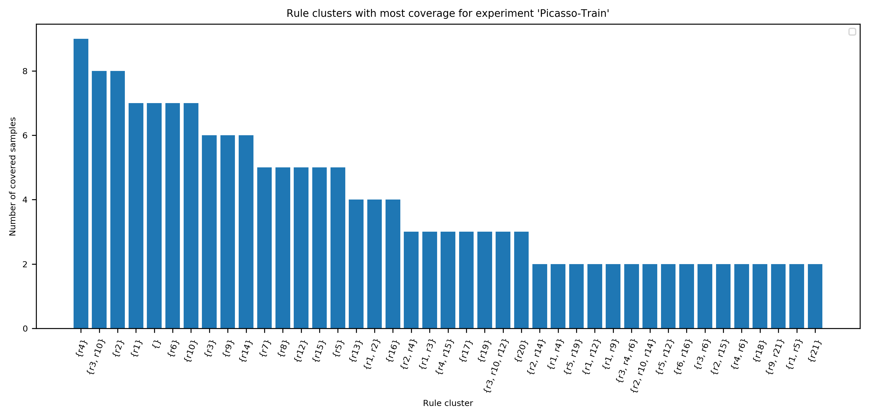
Figure 7: Rule clusters with most coverage for experiment ’Picasso-Train’. Clusters with a frequency of 1 are omitted for better readability. There were 89 such clusters

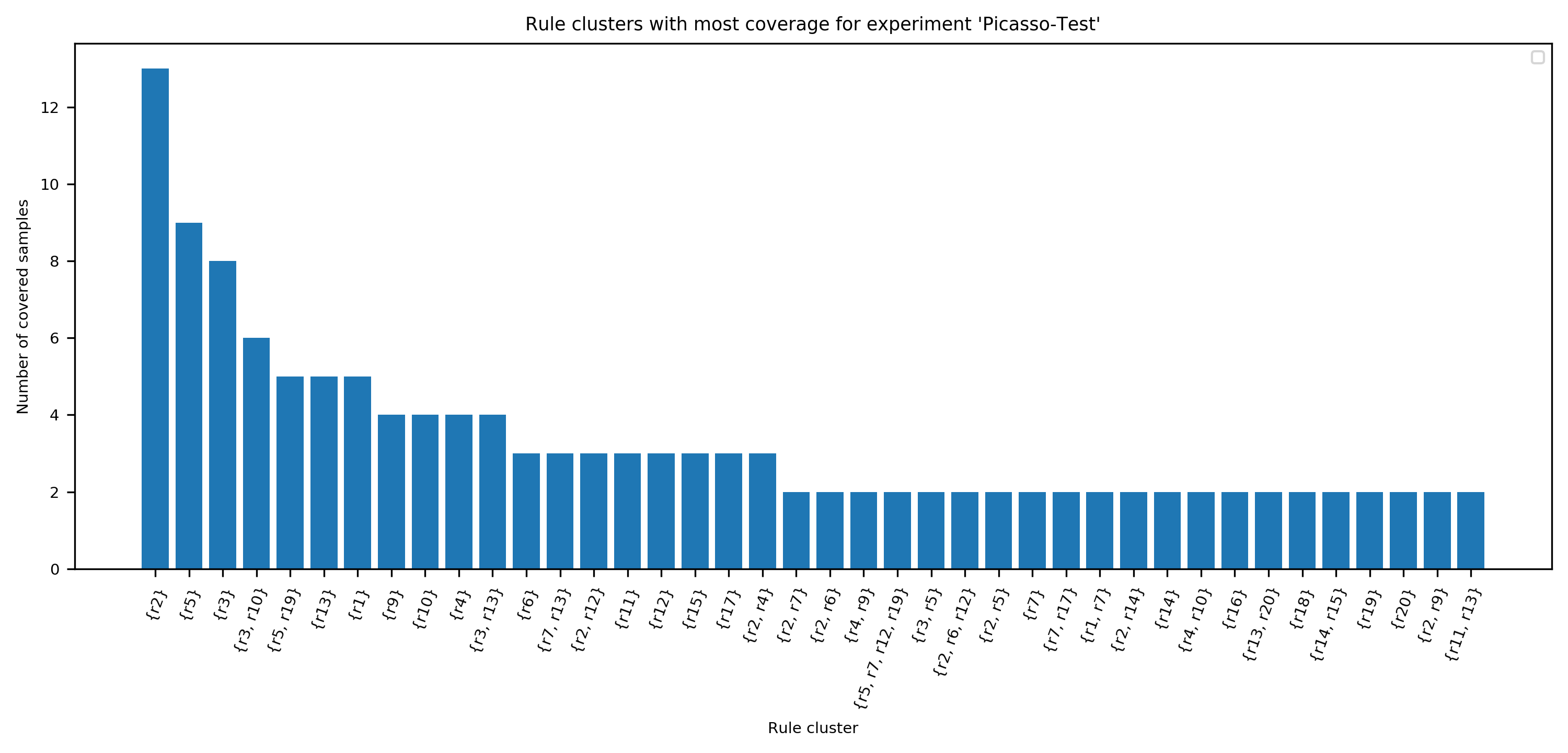
Figure 8: Rule clusters with most coverage for experiment ’Picasso-Test’. Clusters with a frequency of 1 are omitted for better readability. There were 117 such clusters

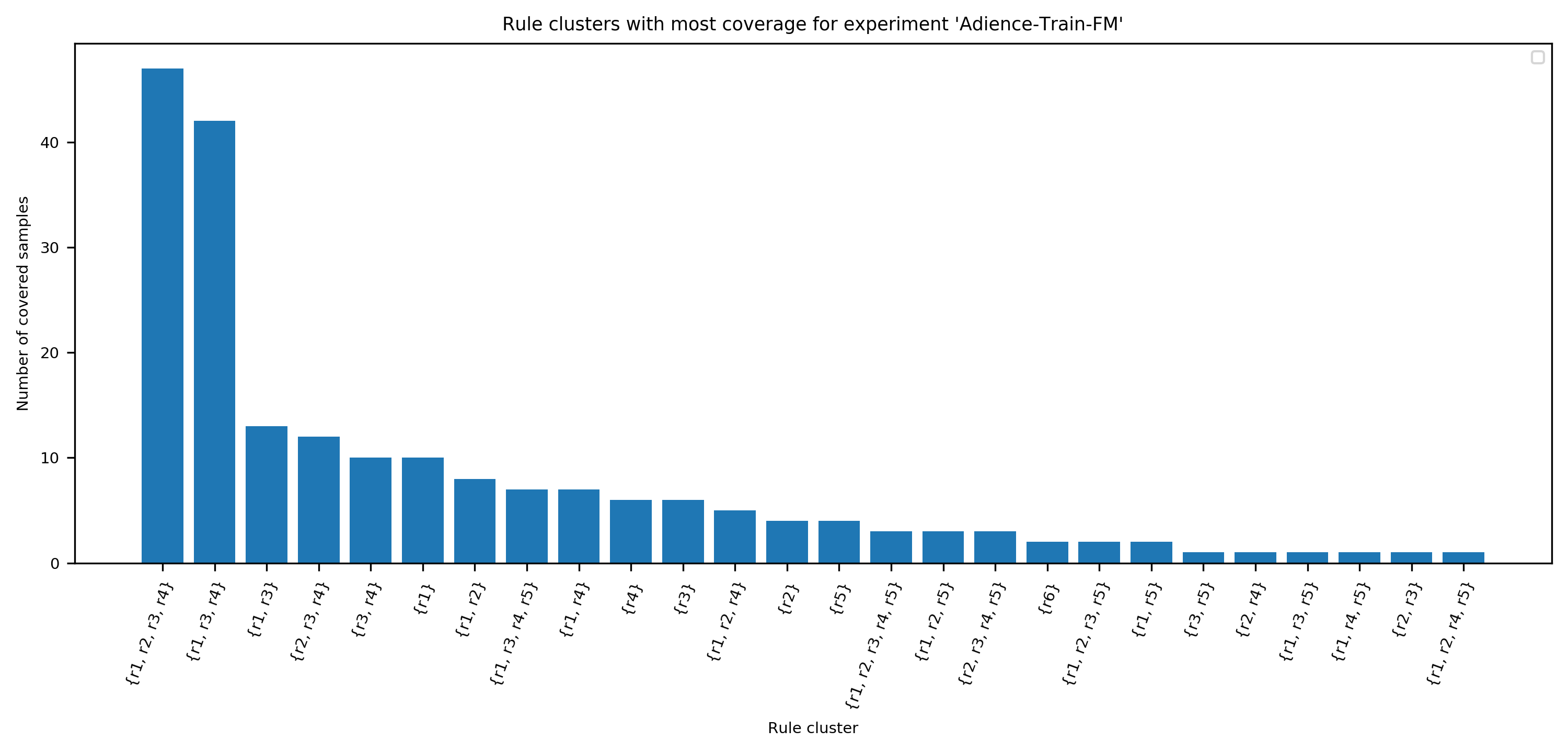
Figure 9: Rule clusters with most coverage for experiment ’Adience-Train-FM’

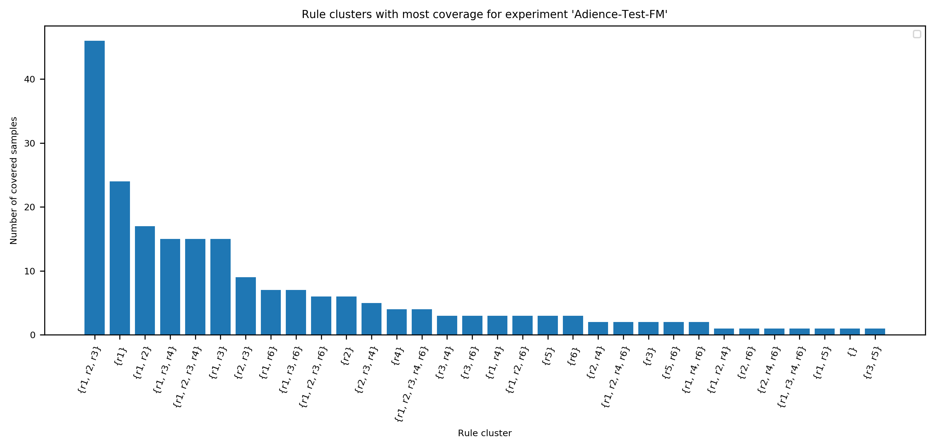
Figure 10: Rule clusters with most coverage for experiment ’Adience-Test-FM’

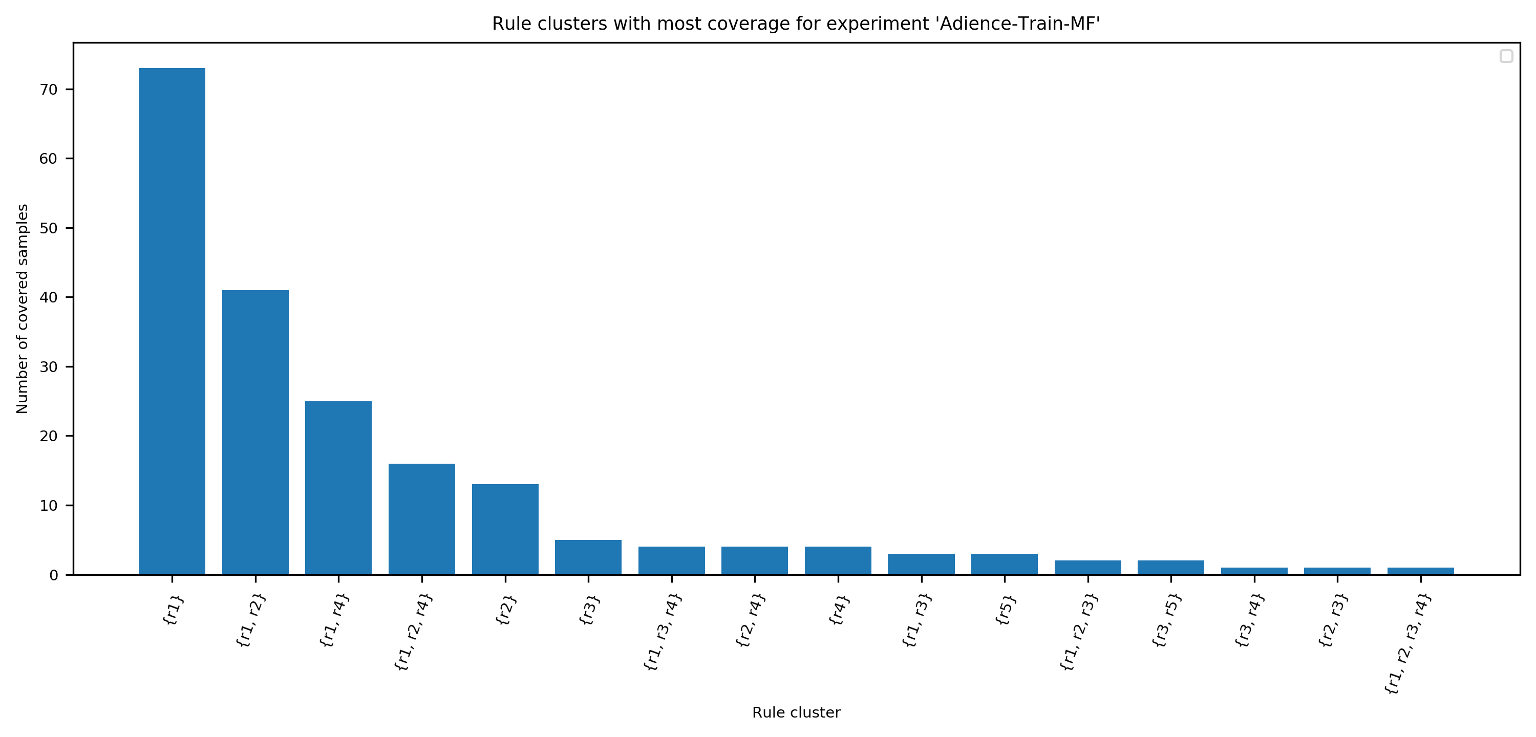
Figure 11: Rule clusters with most coverage for experiment ’Adience-Train-MF’

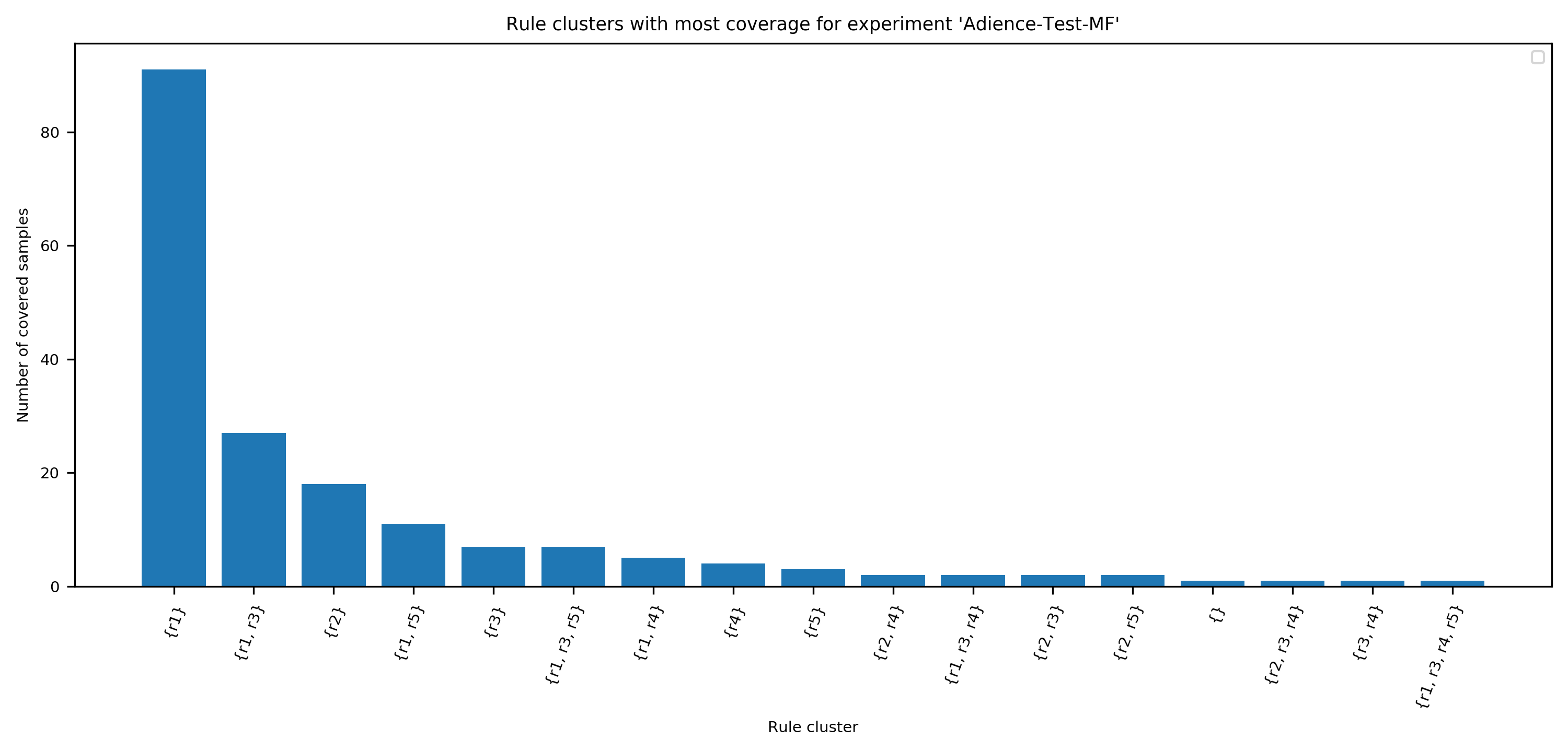
Figure 12: Rule clusters with most coverage for experiment ’Adience-Test-MF’

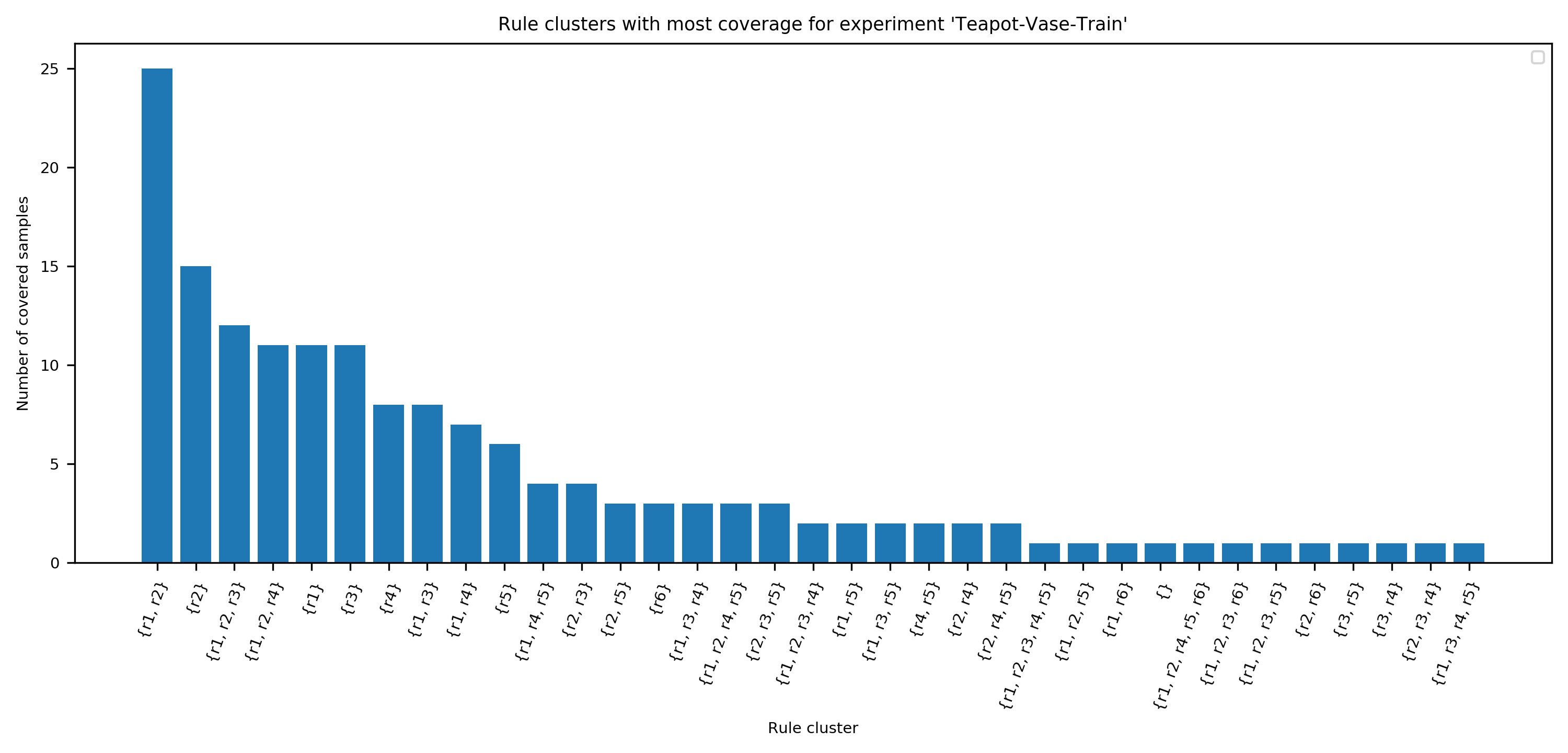
Figure 13: Rule clusters with most coverage for experiment ’Teapot-Vase-Train’

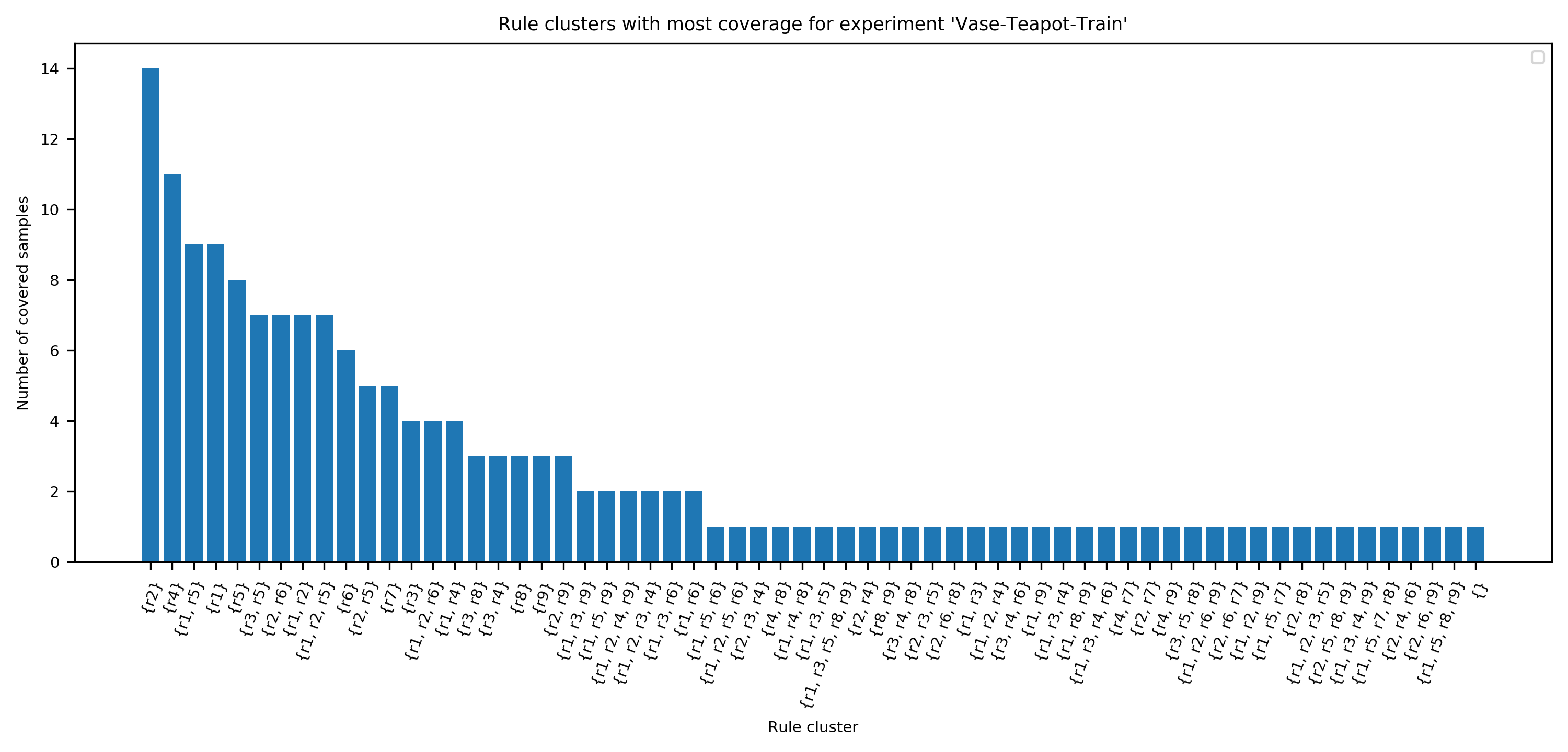
Figure 14: Rule clusters with most coverage for experiment ’Vase-Teapot-Train’

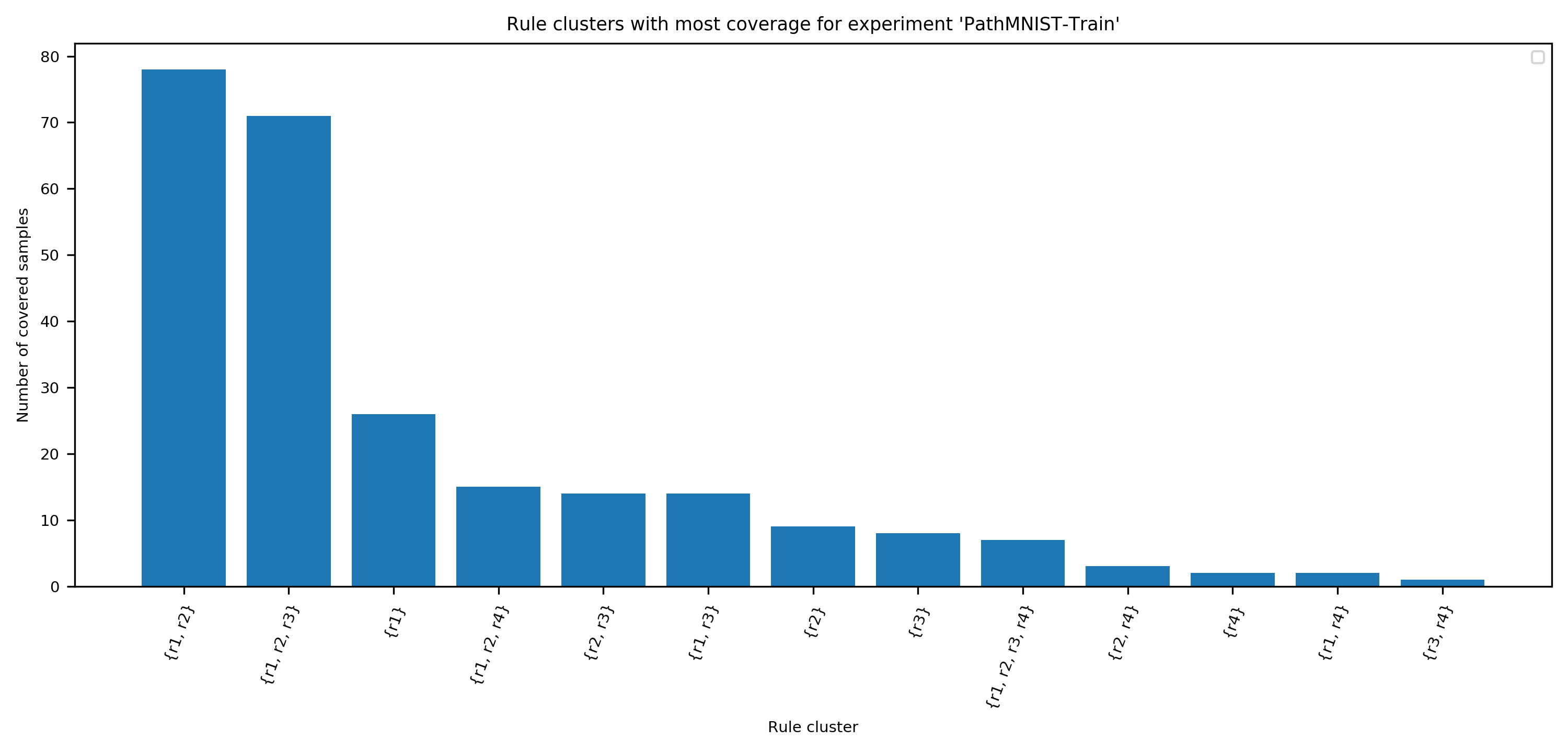
Figure 15: Rule clusters with most coverage for experiment ’PathMNIST-Train’

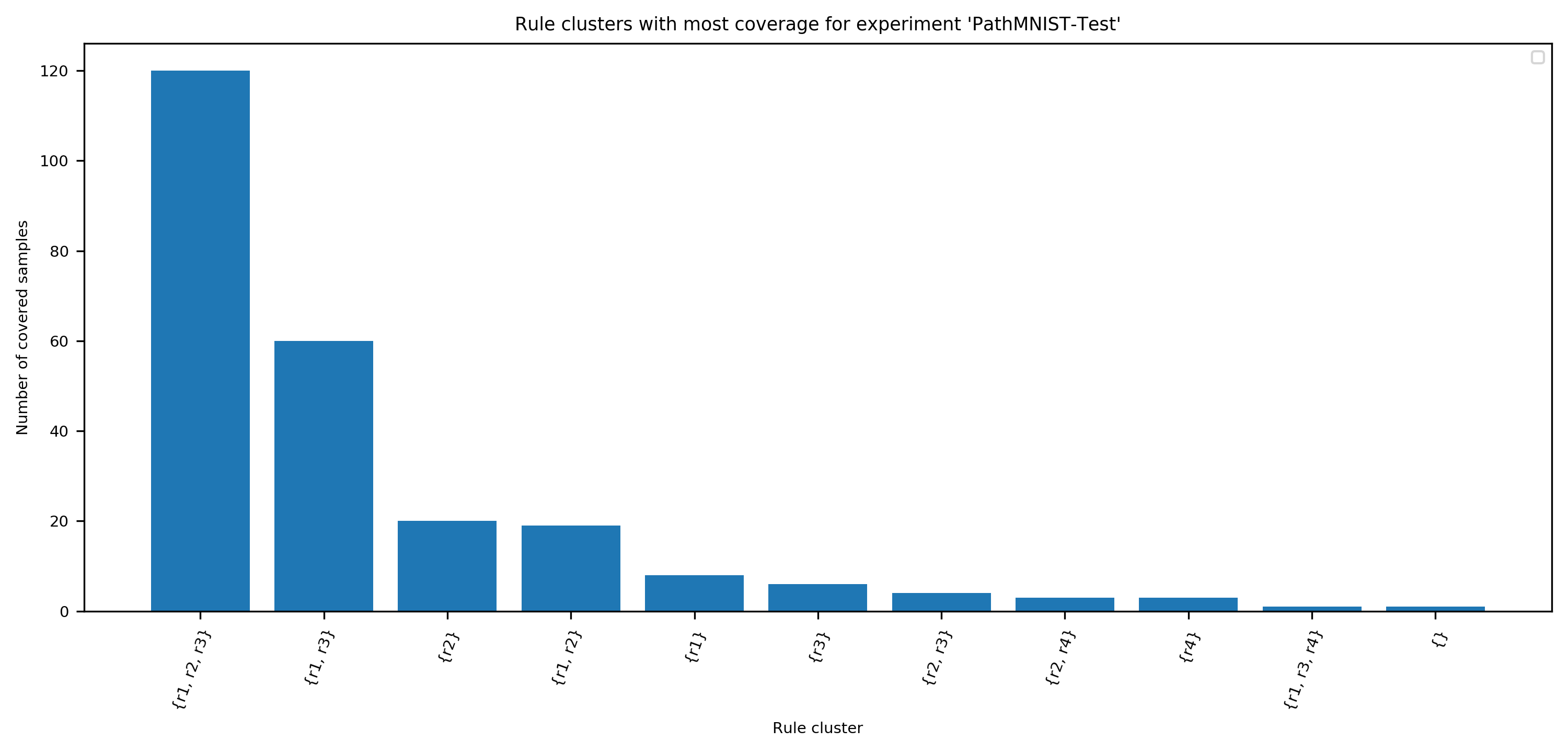
Figure 16: Rule clusters with most coverage for experiment ’PathMNIST-Test’

Appendix D Frequency of concepts from top-3 rules per concept rank

The Figures 17, 18, 19, 20, 21, 22, 23, 24, 25, 26 show occurrences of concepts from top-3 rules (the 3 rules with the highest coverage of examples) given per concept rank. The ranking stems from the absolute value of the concept relevance. The x-axis shows the 10 ranks a given concept was ranked most frequently, calculated over all samples in a data set. Typically, high rankings (low numbers) in the 10 most occurring ranks are expected.

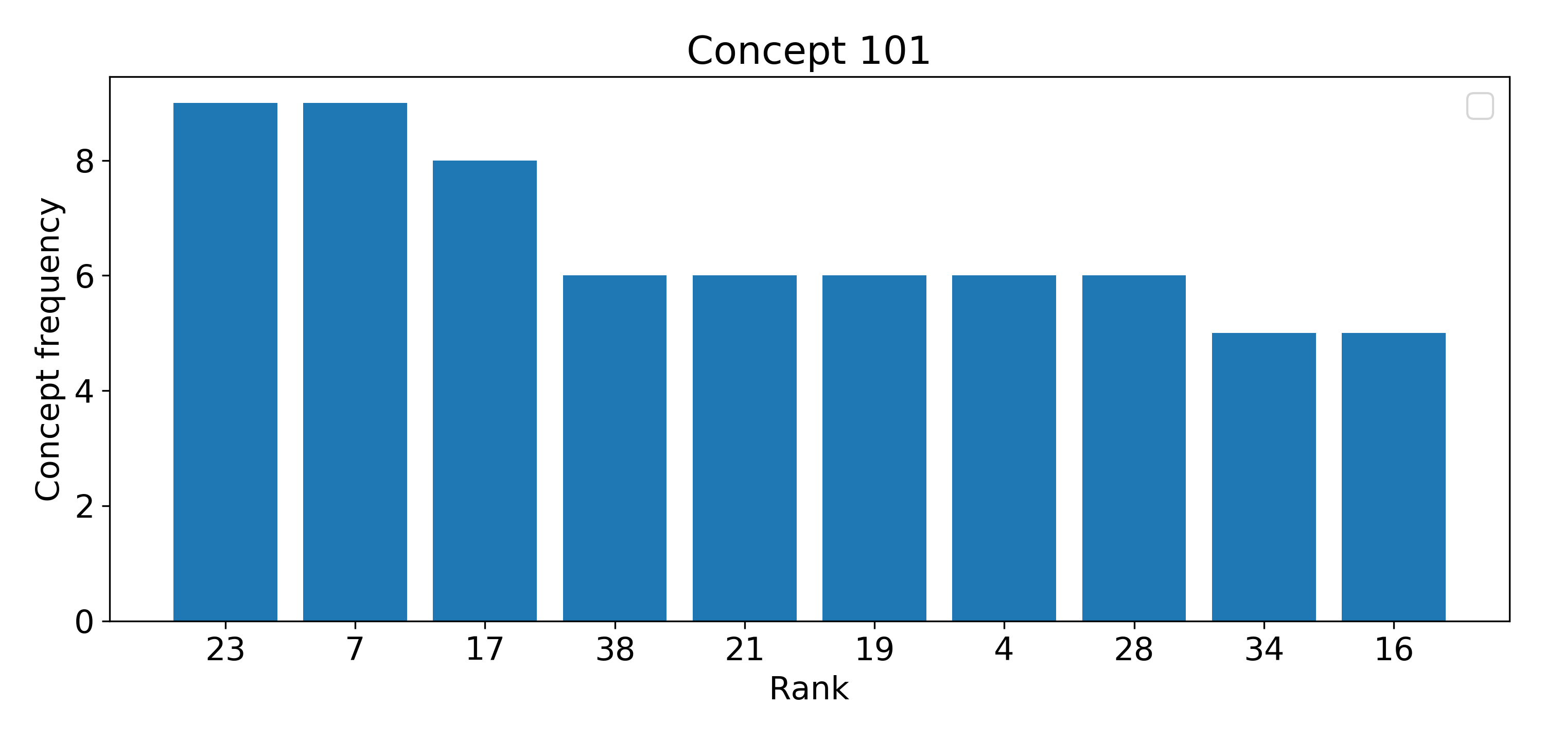
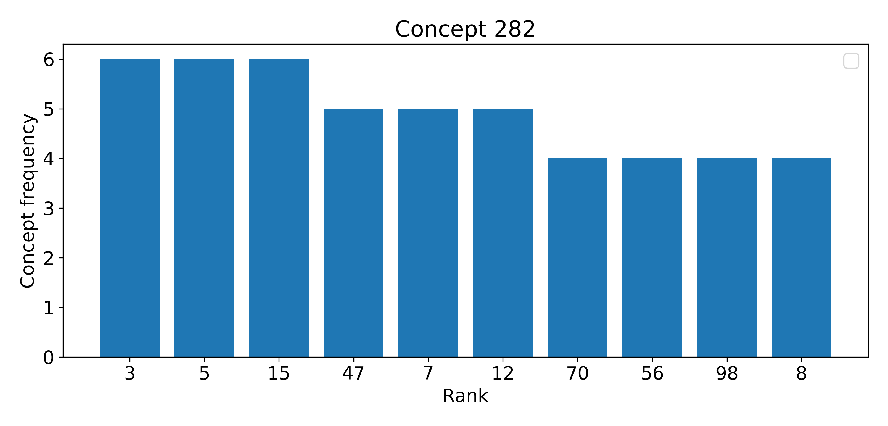
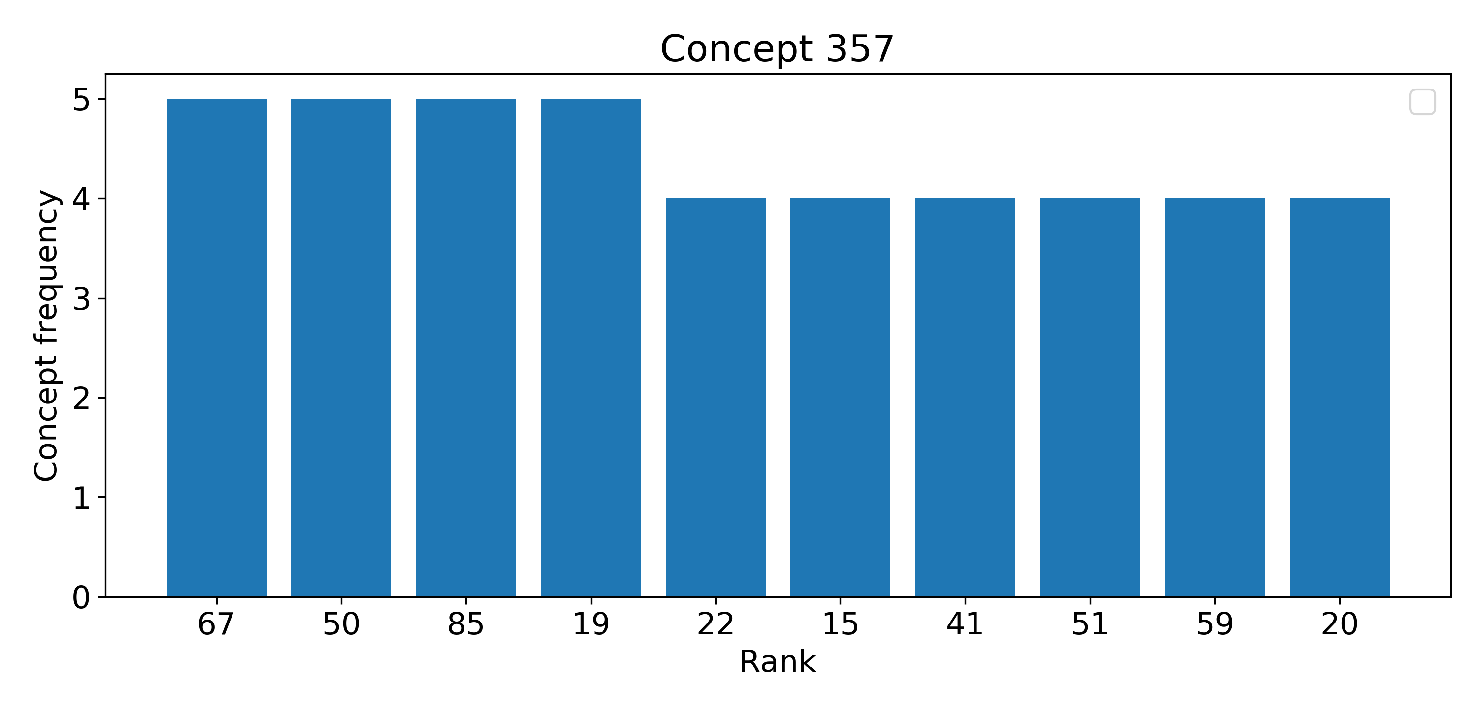
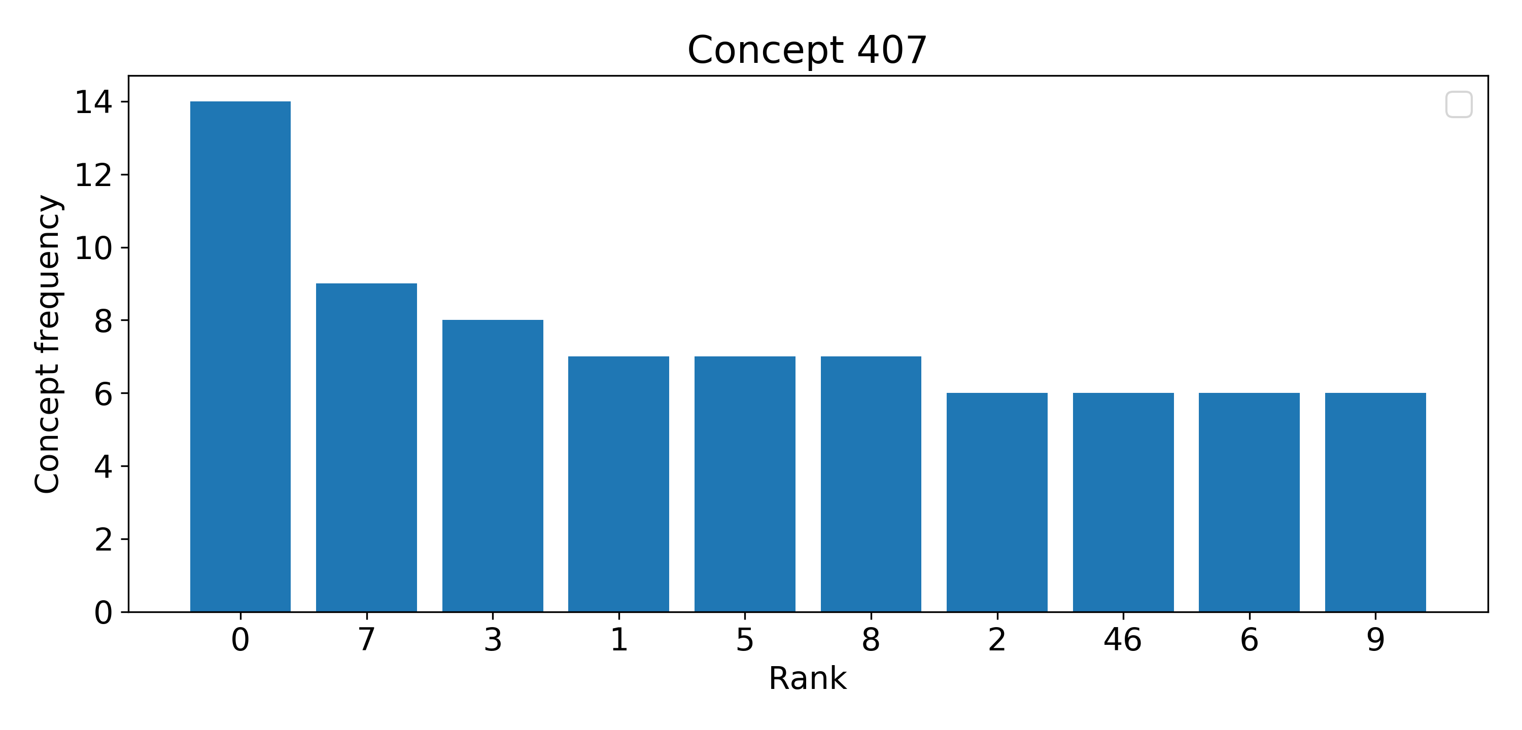
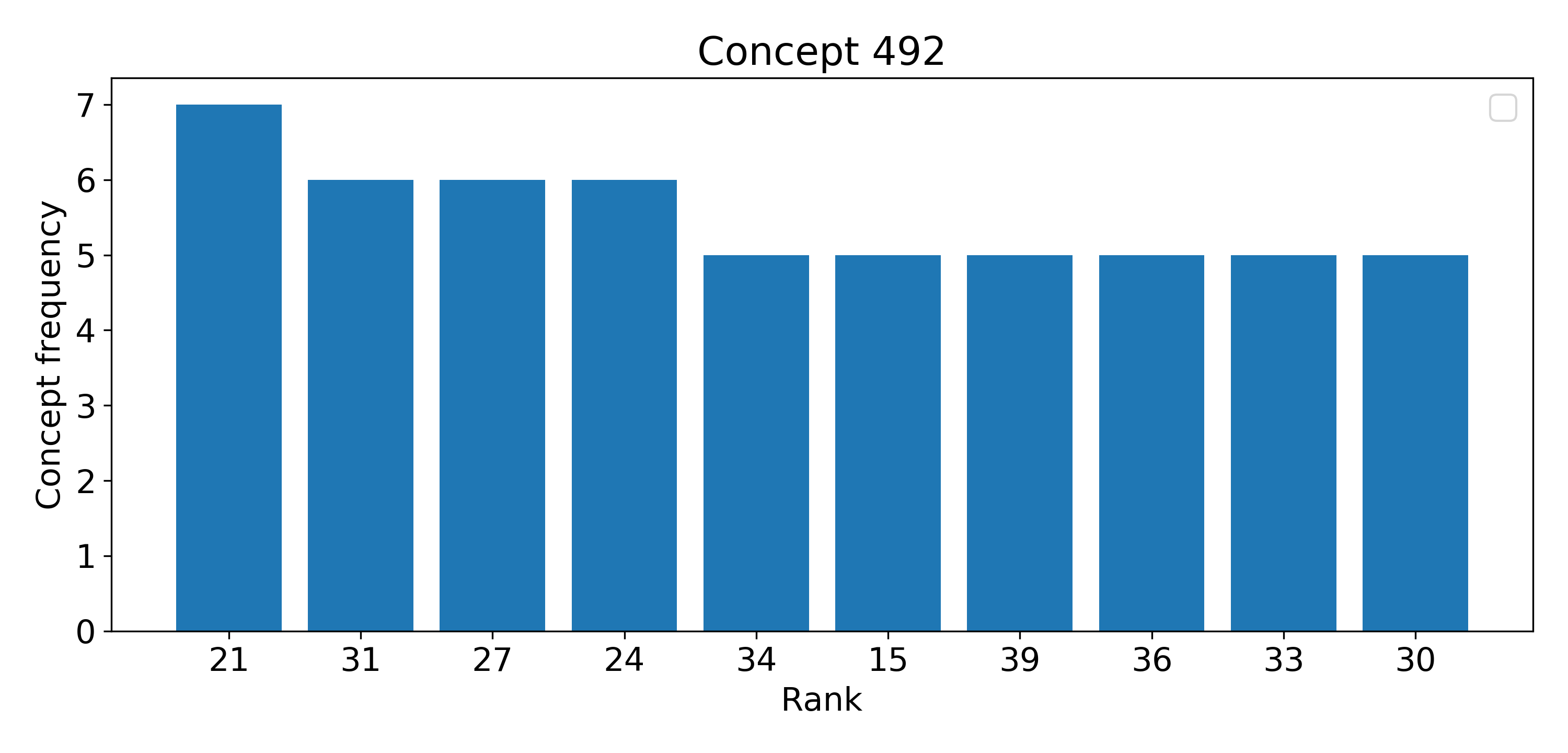
Figure 17: Ranks that are reached the most over all samples for the top-3 rule concepts for experiment ’Picasso-Train’. The 3 rules with the most covered samples (sample count in bold) are:
(44) Face, if concept 357 above of concept 407
(43) Face, if concept 407 is right of concept 101
(40) Face, if concept 492 is below concept 282

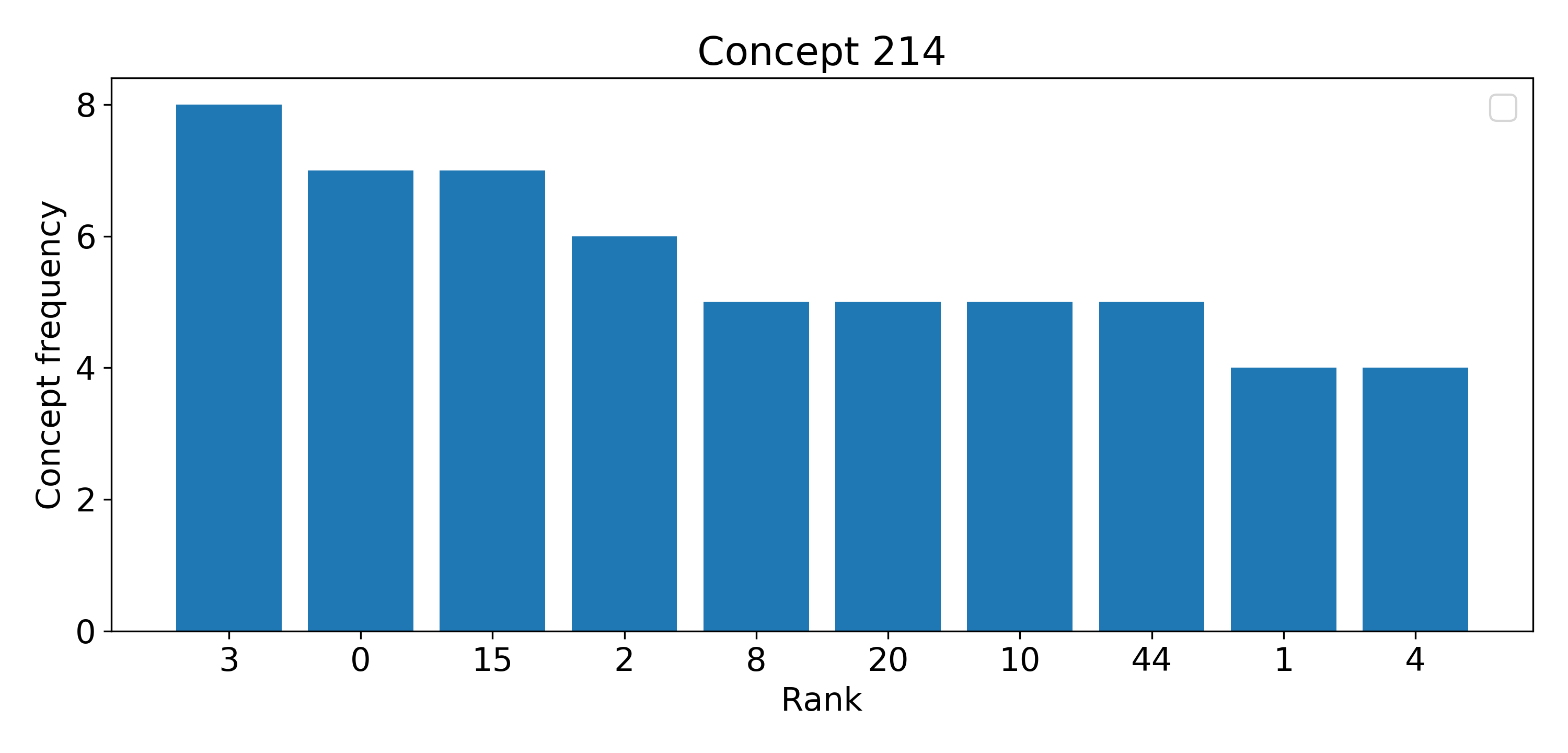
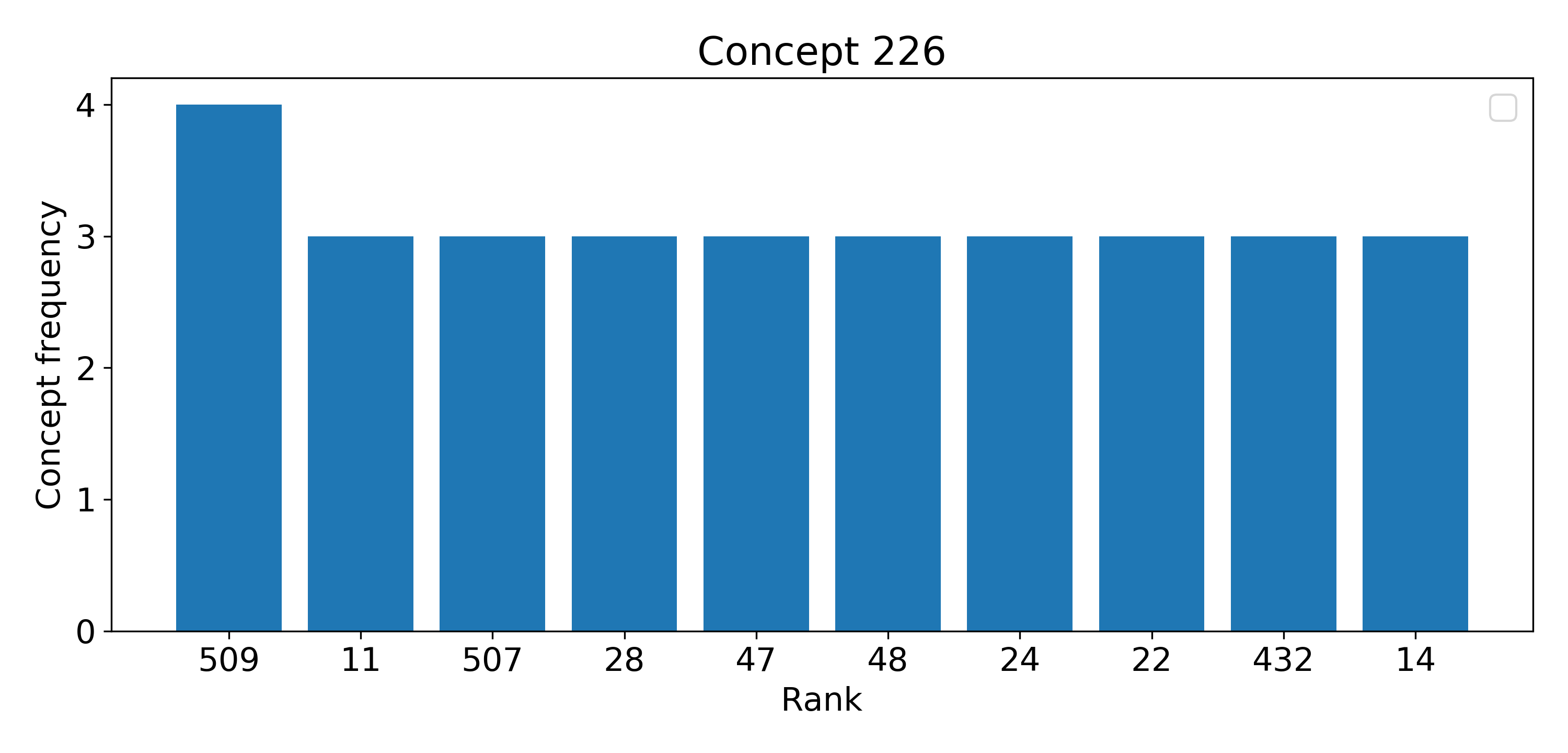
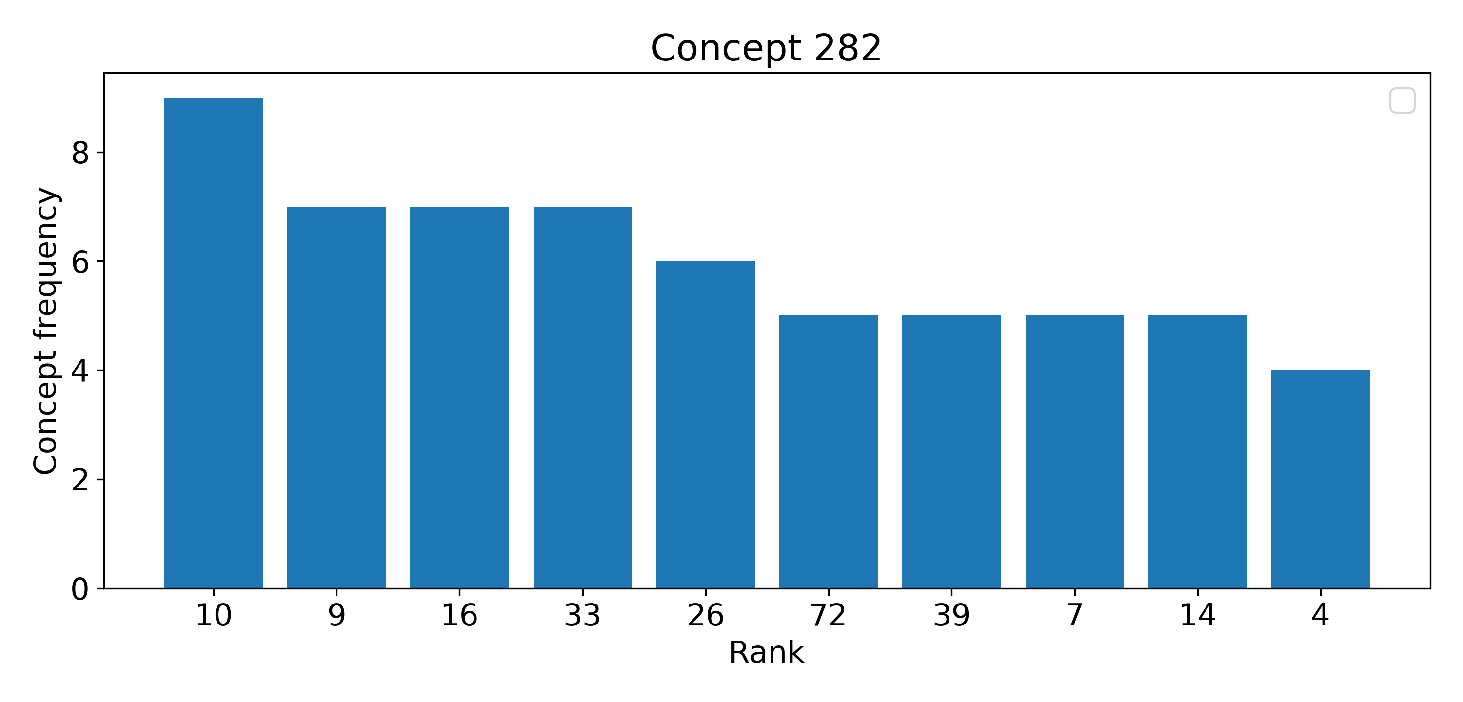
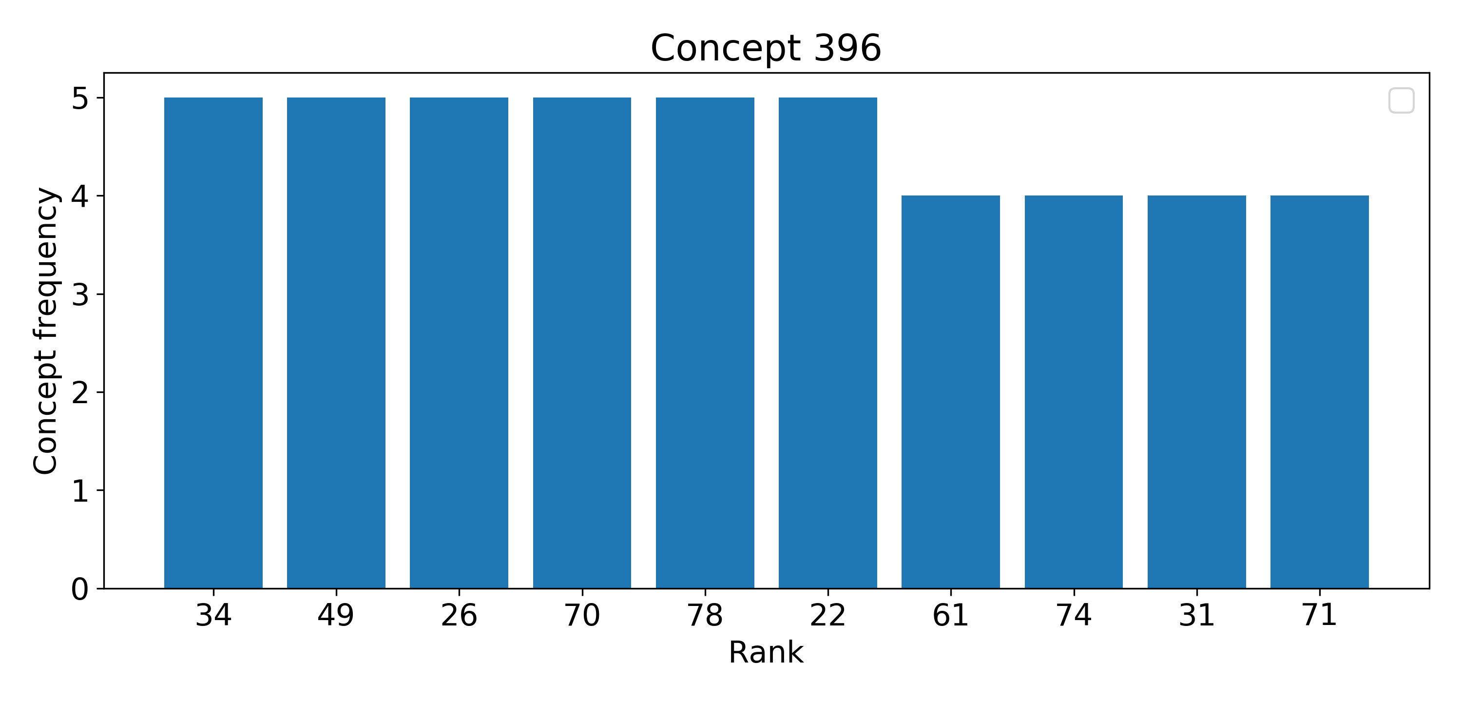
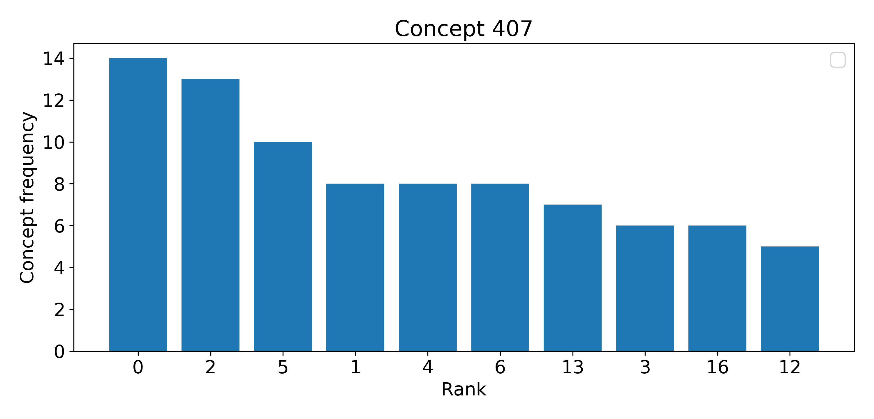
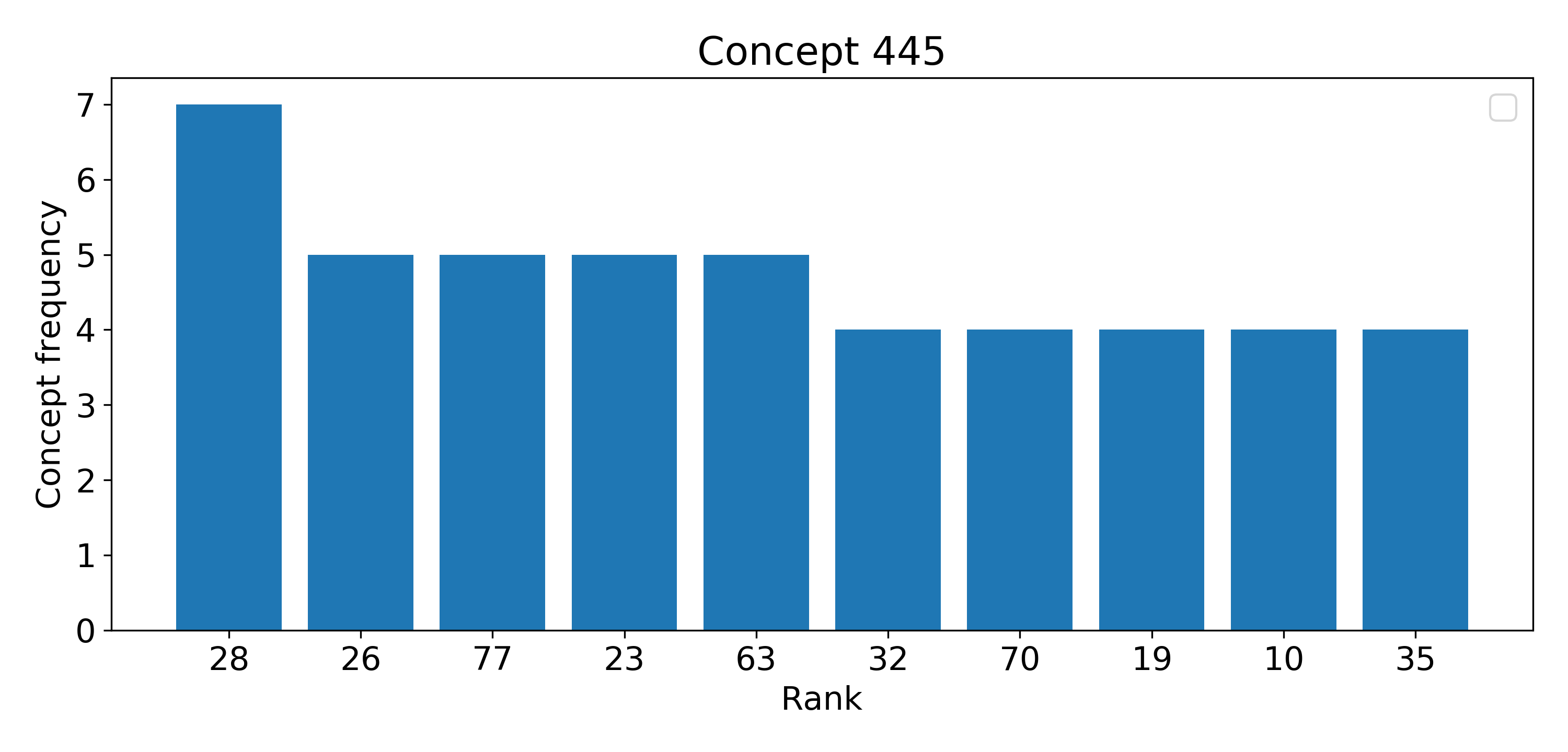
Figure 18: Ranks that are reached the most over all samples for the top-3 rule concepts for experiment ’Picasso-Test’. The 3 rules with the most covered samples (sample count in bold) are:
(62) Face, if concept 282 is above of concept 396
(52) Face, if concept 226 is above of concept 407
(40) Face, if concept 214 is below concept 445

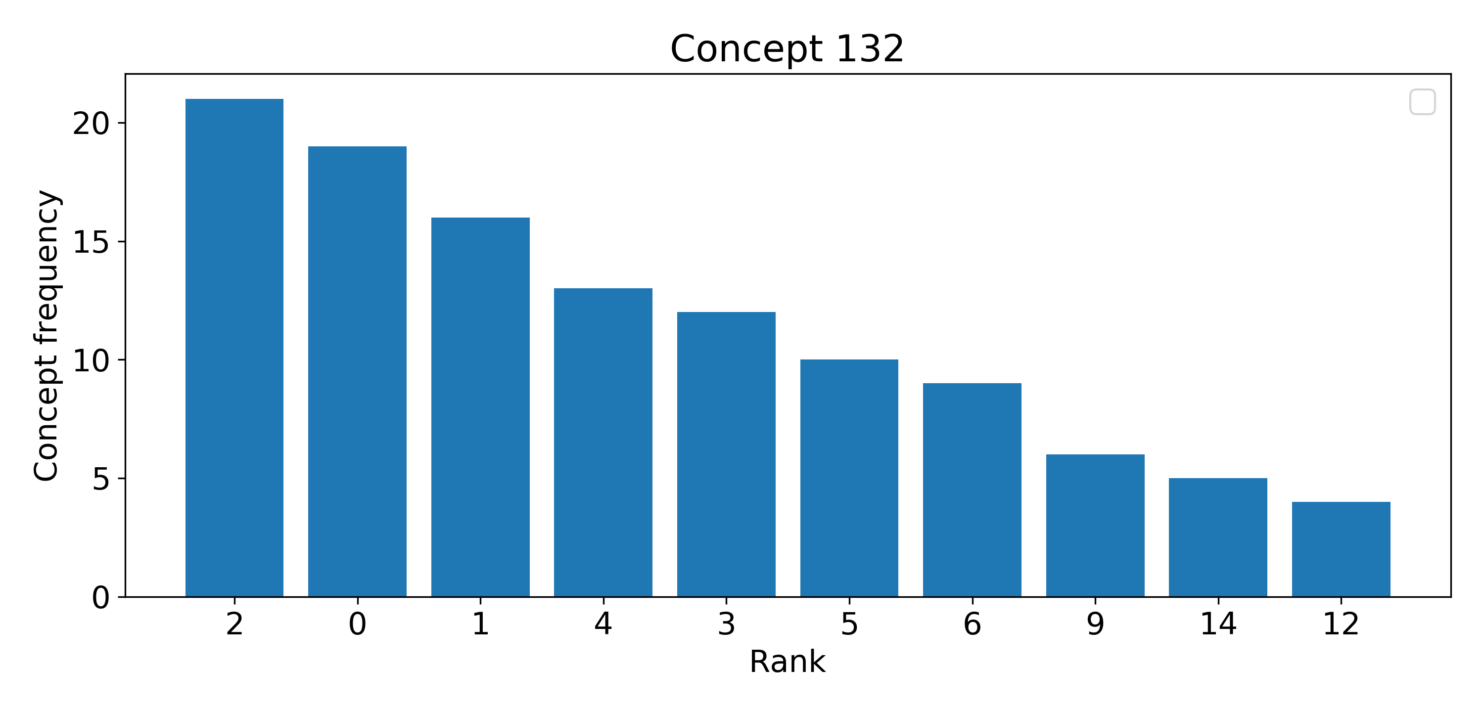
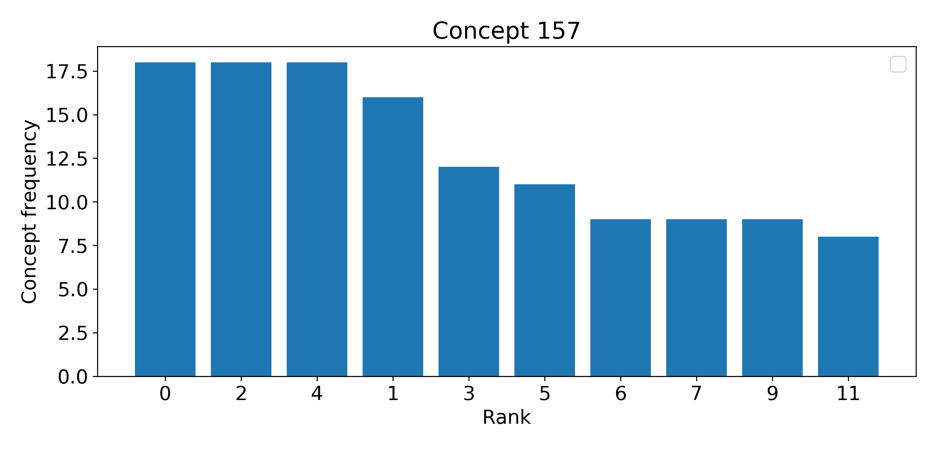
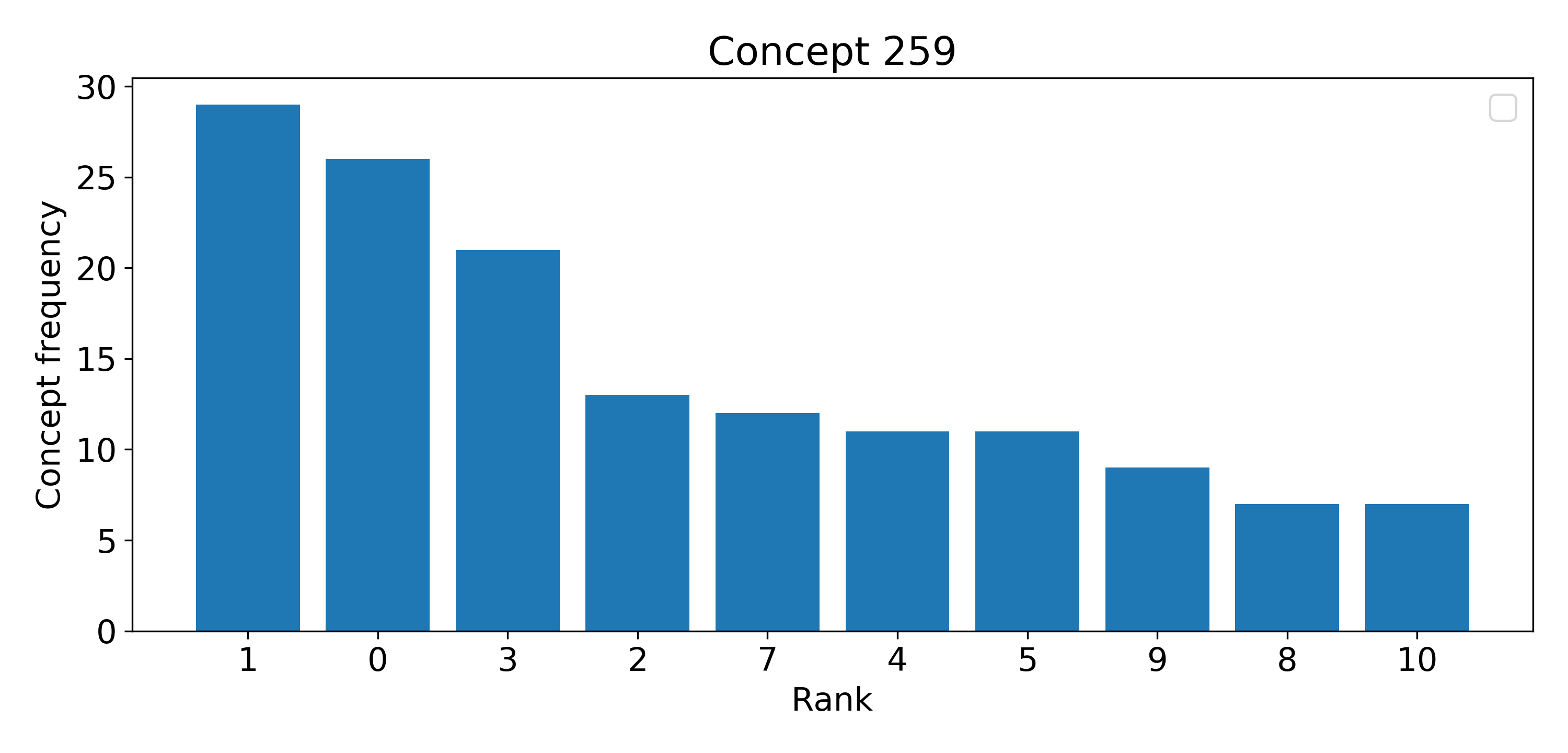
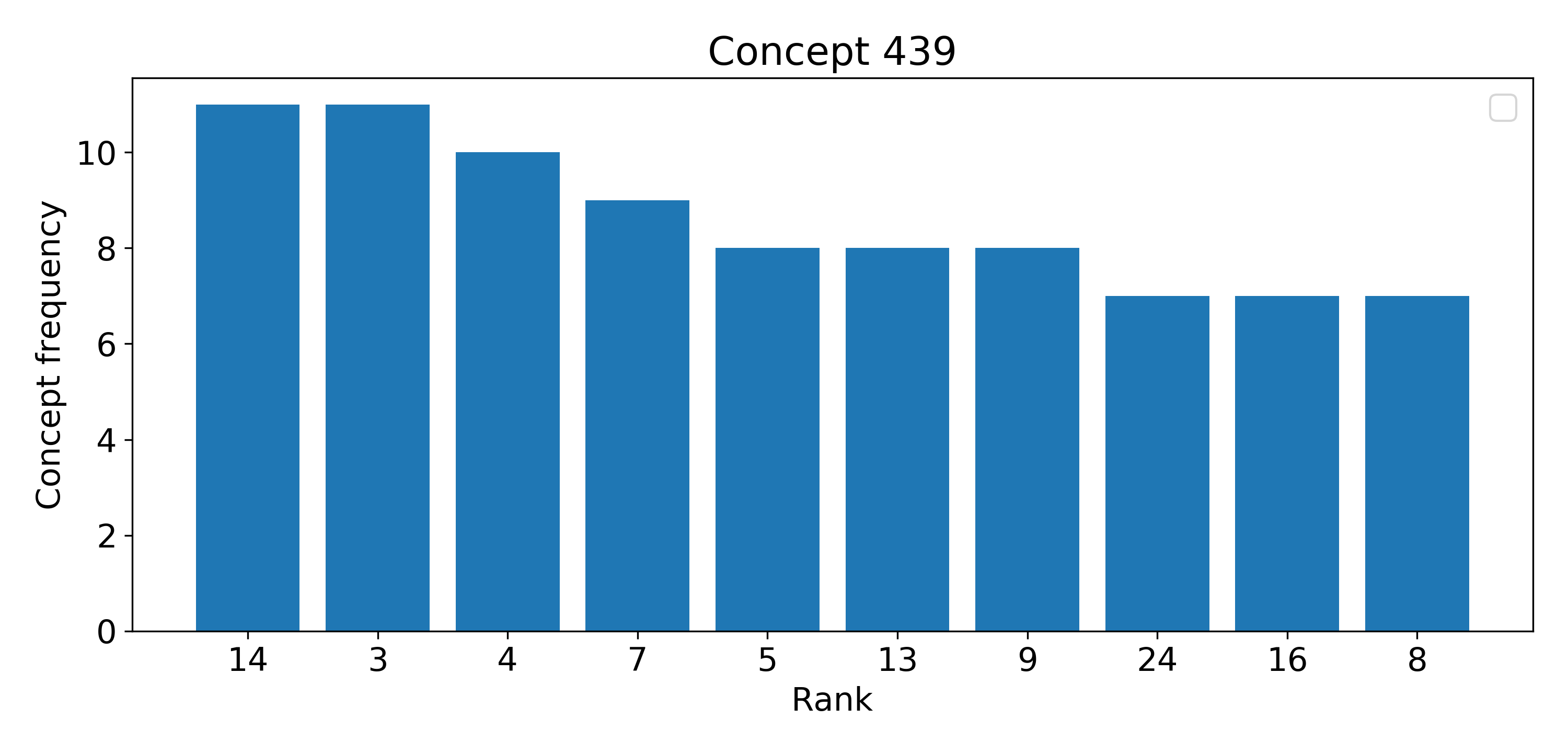
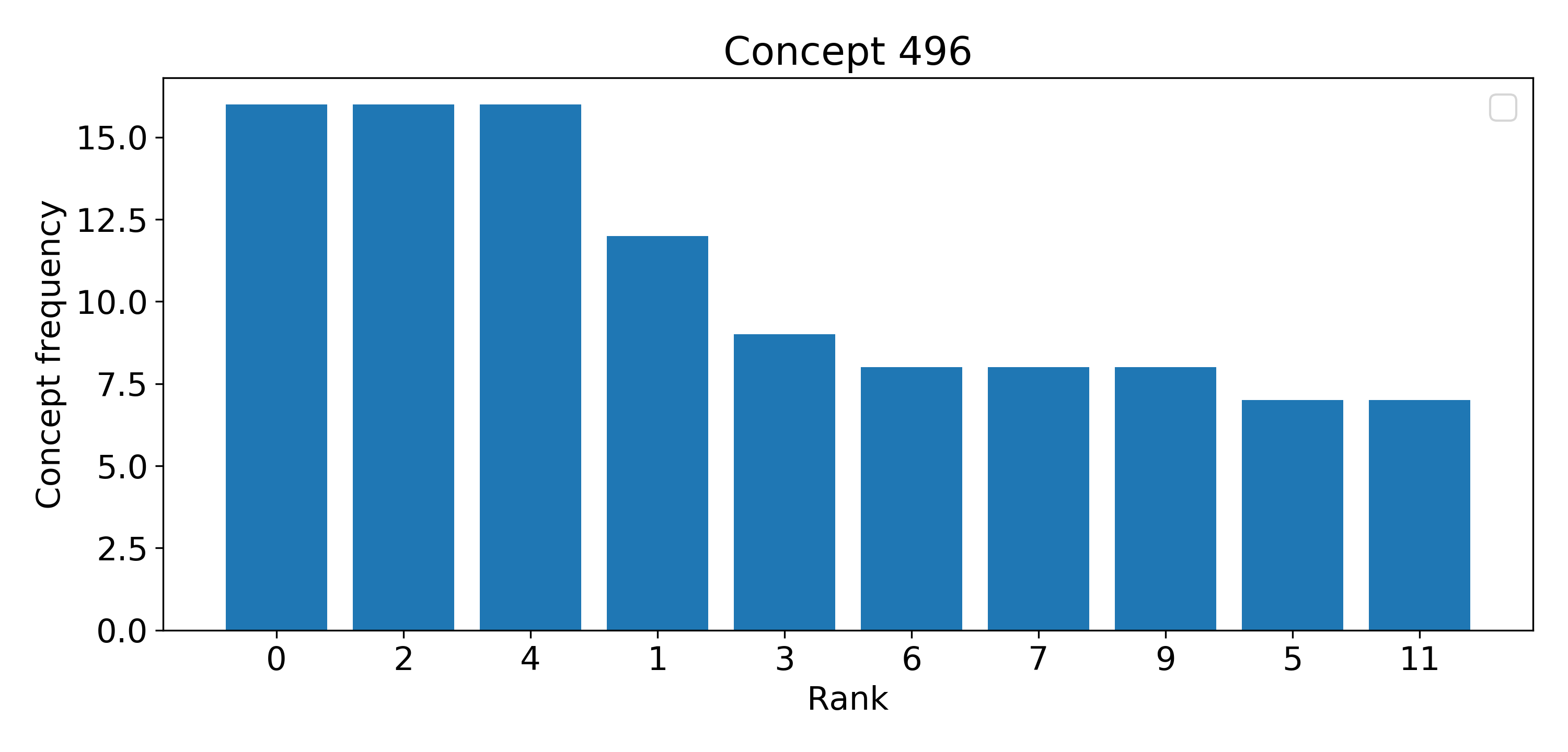
Figure 19: Ranks that are reached the most over all samples for the top-3 rule concepts for experiment ’Adience-Train-FM’. The 3 rules with the most covered samples (sample count in bold) are:
(152) Female, if concept 259 is above of concept 439
(148) Female, if concept 132 is above of concept 496
(145) Female, if concept 157 is above of concept 496

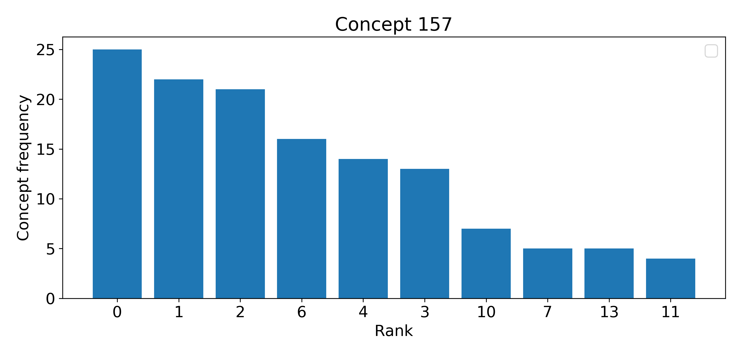
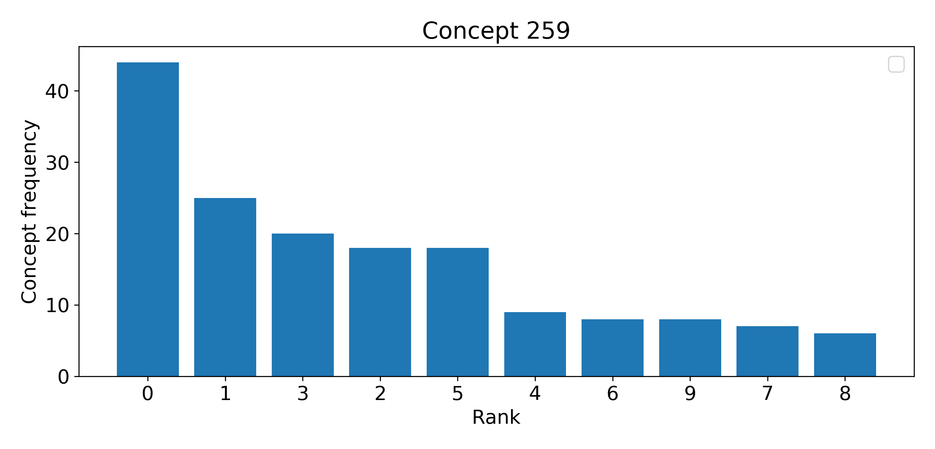
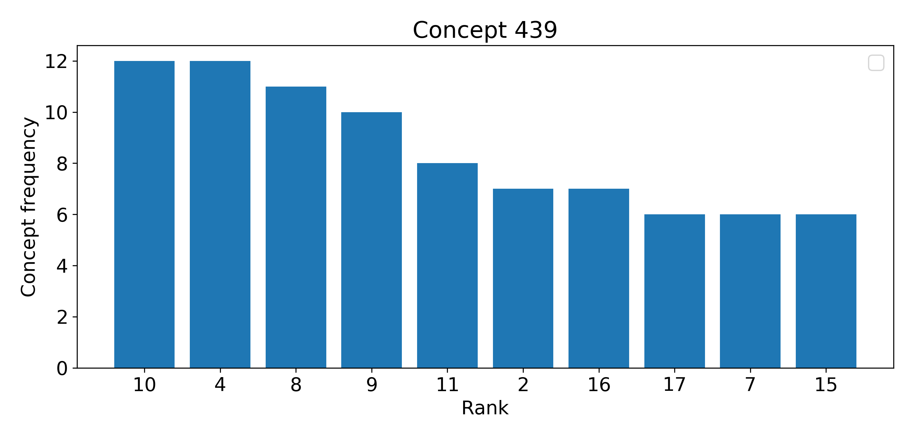
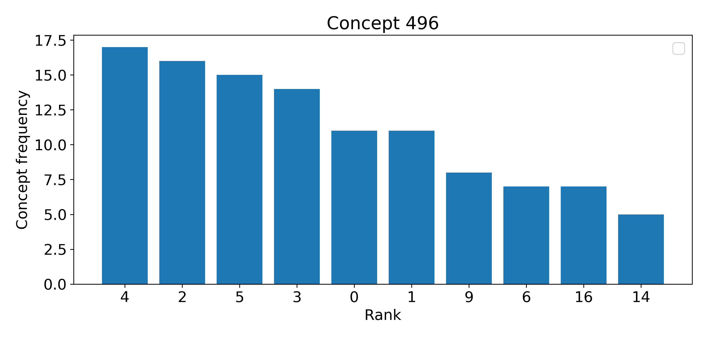
Figure 20: Ranks that are reached the most over all samples for the top-3 rule concepts for experiment ’Adience-Test-FM’. The 3 rules with the most covered samples (sample count in bold) are:
(169) Female, if concept 259 is above of concept 496
(132) Female, if concept 157 is left of concept 259
(118) Female, if concept 157 is above of concept 439

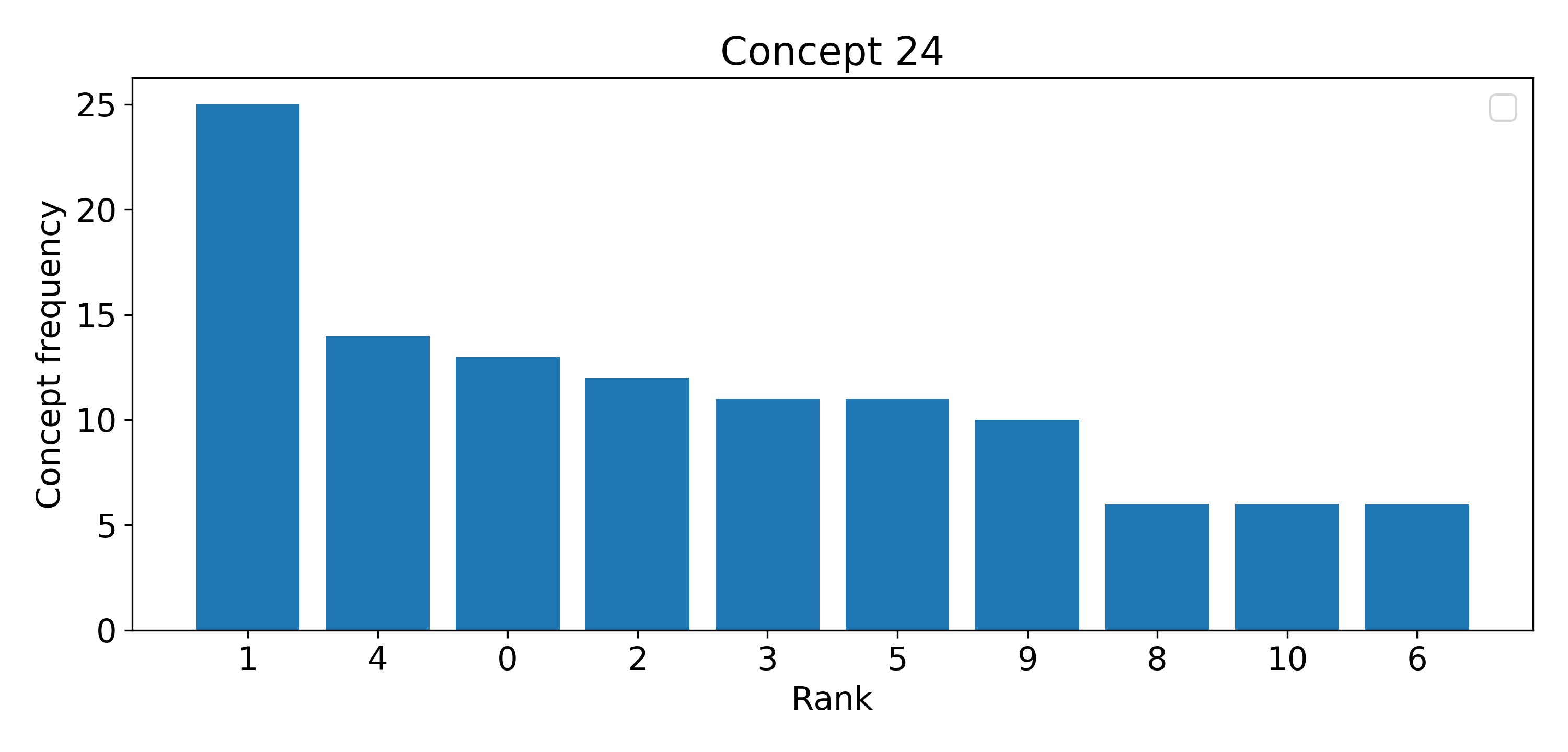
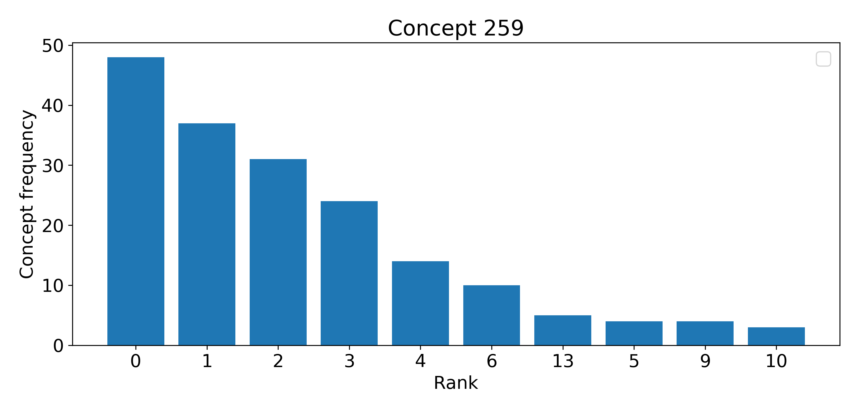
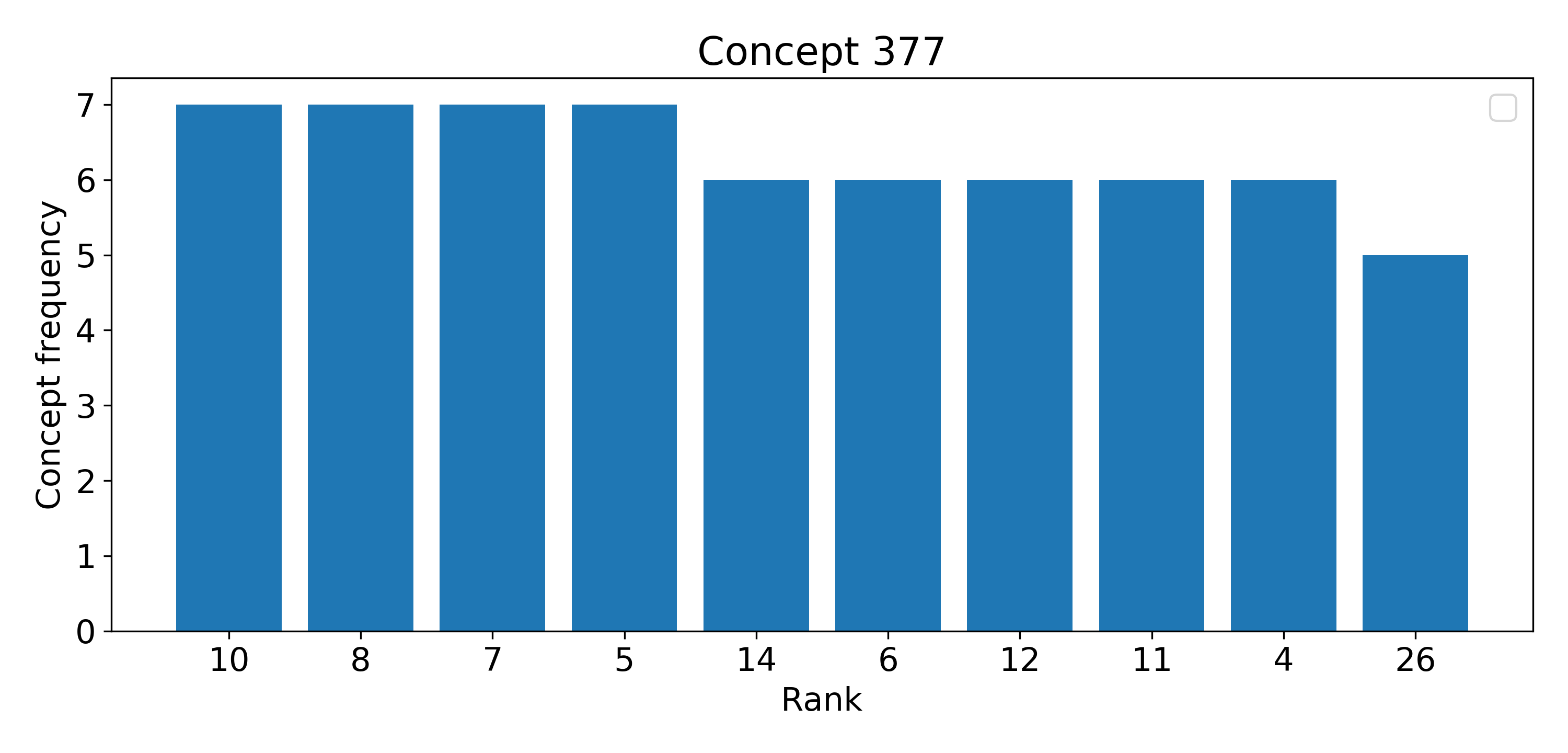
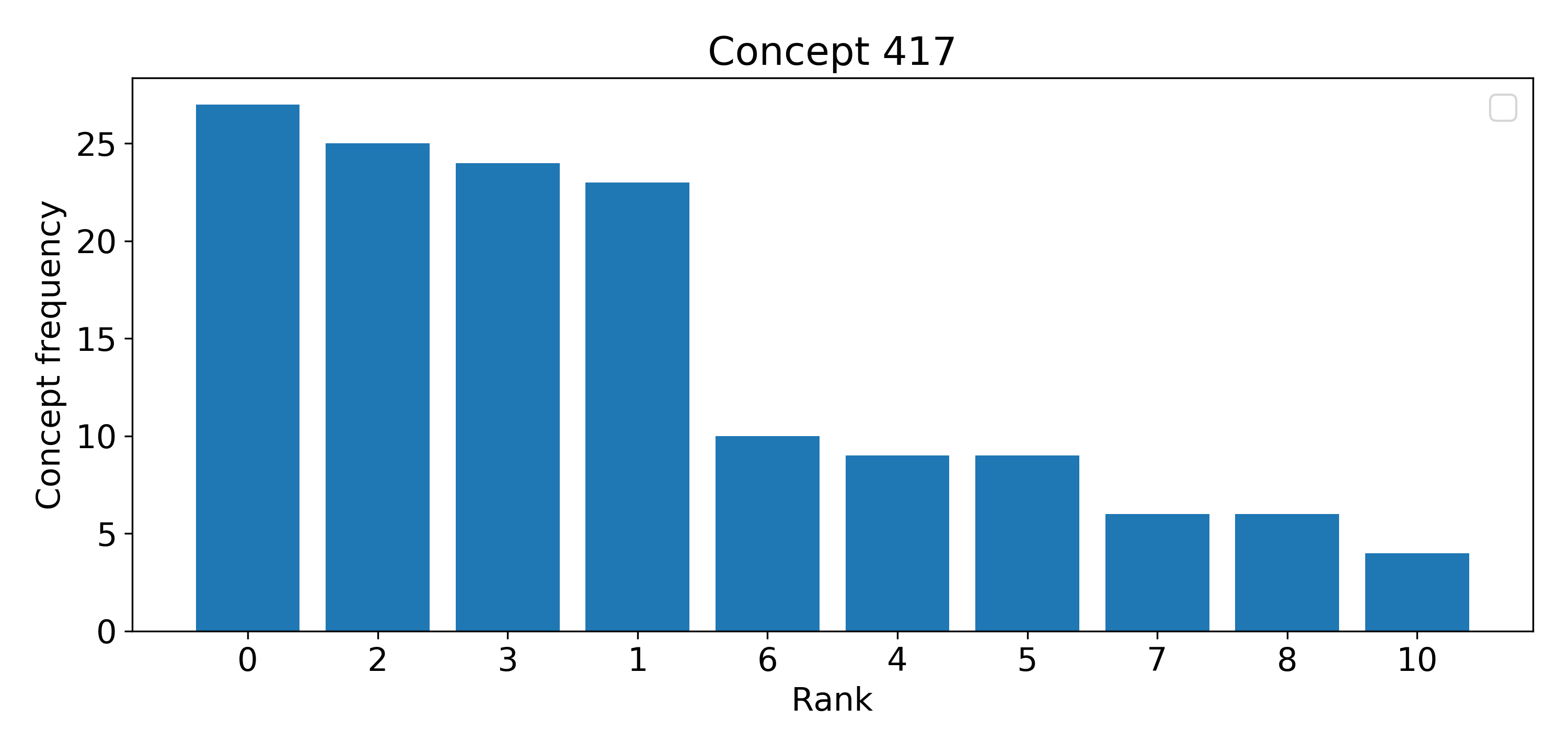
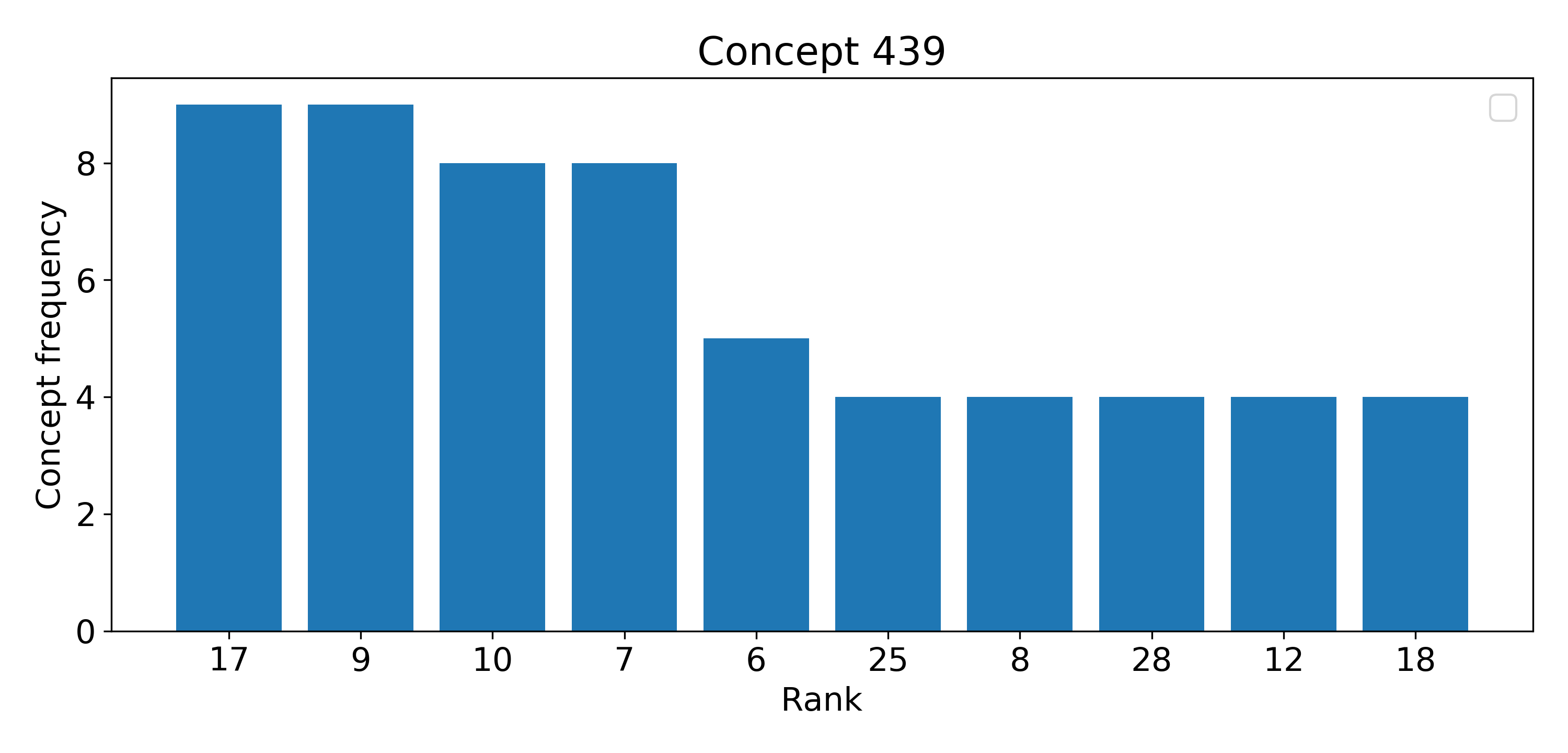
Figure 21: Ranks that are reached the most over all samples for the top-3 rule concepts for experiment ’Adience-Train-MF’. The 3 rules with the most covered samples (sample count in bold) are:
(165) Male, if concept 259 is above of concept 417
(78) Male, if concept 259 is left of concept 377
(55) Male, if concept 24 is above of concept 439

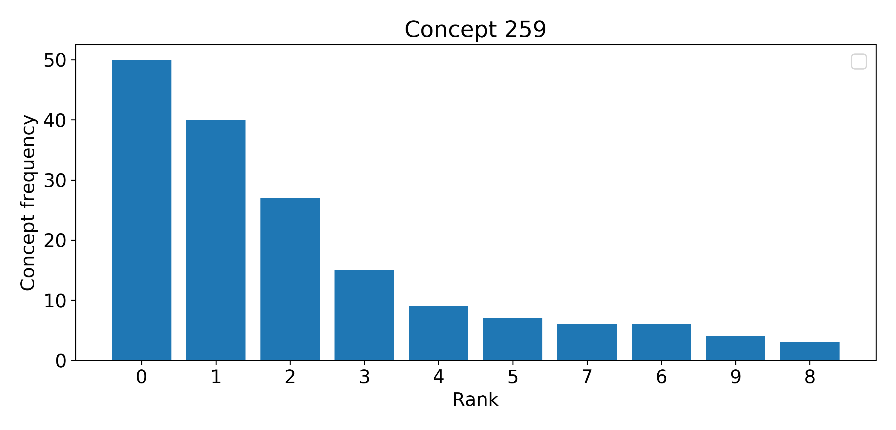
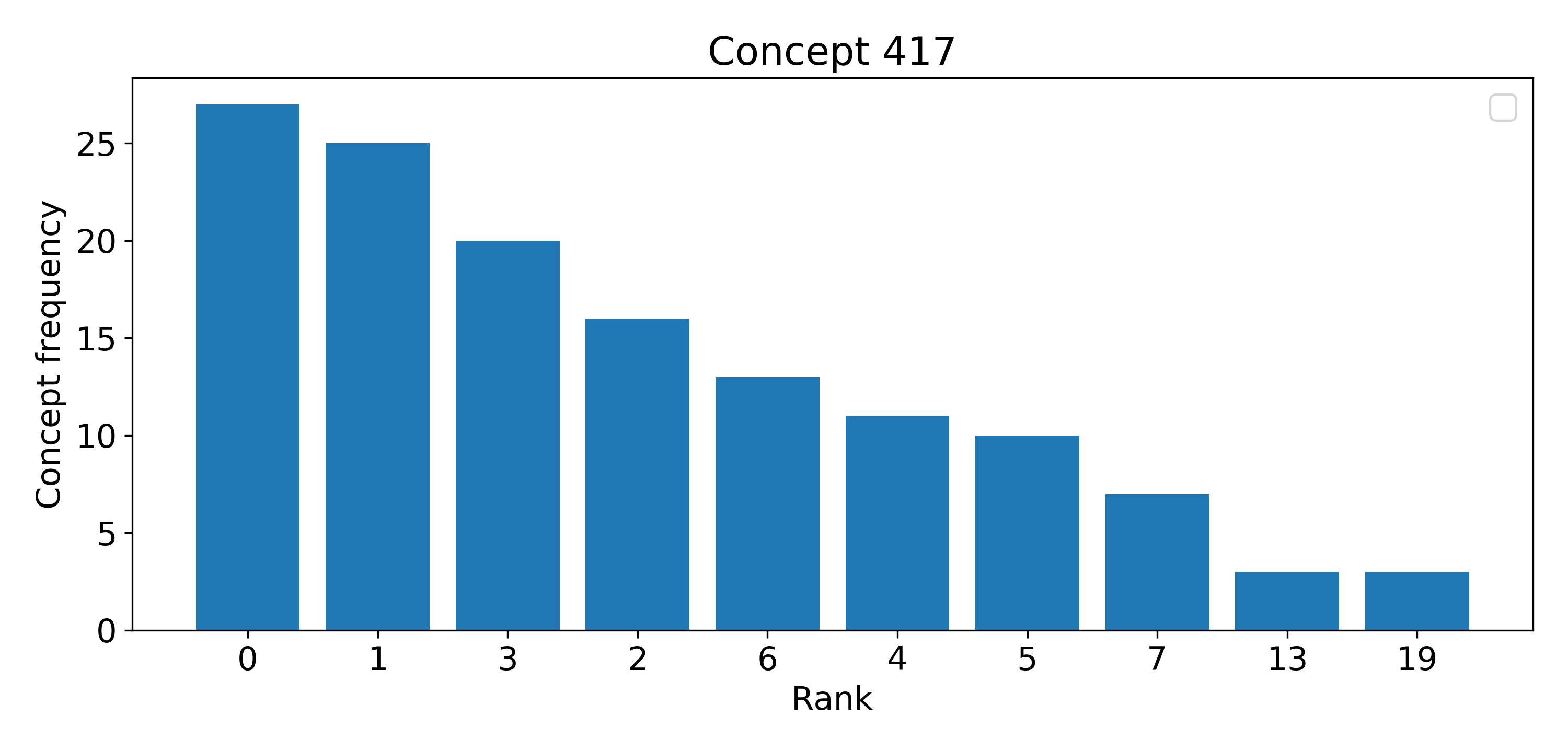
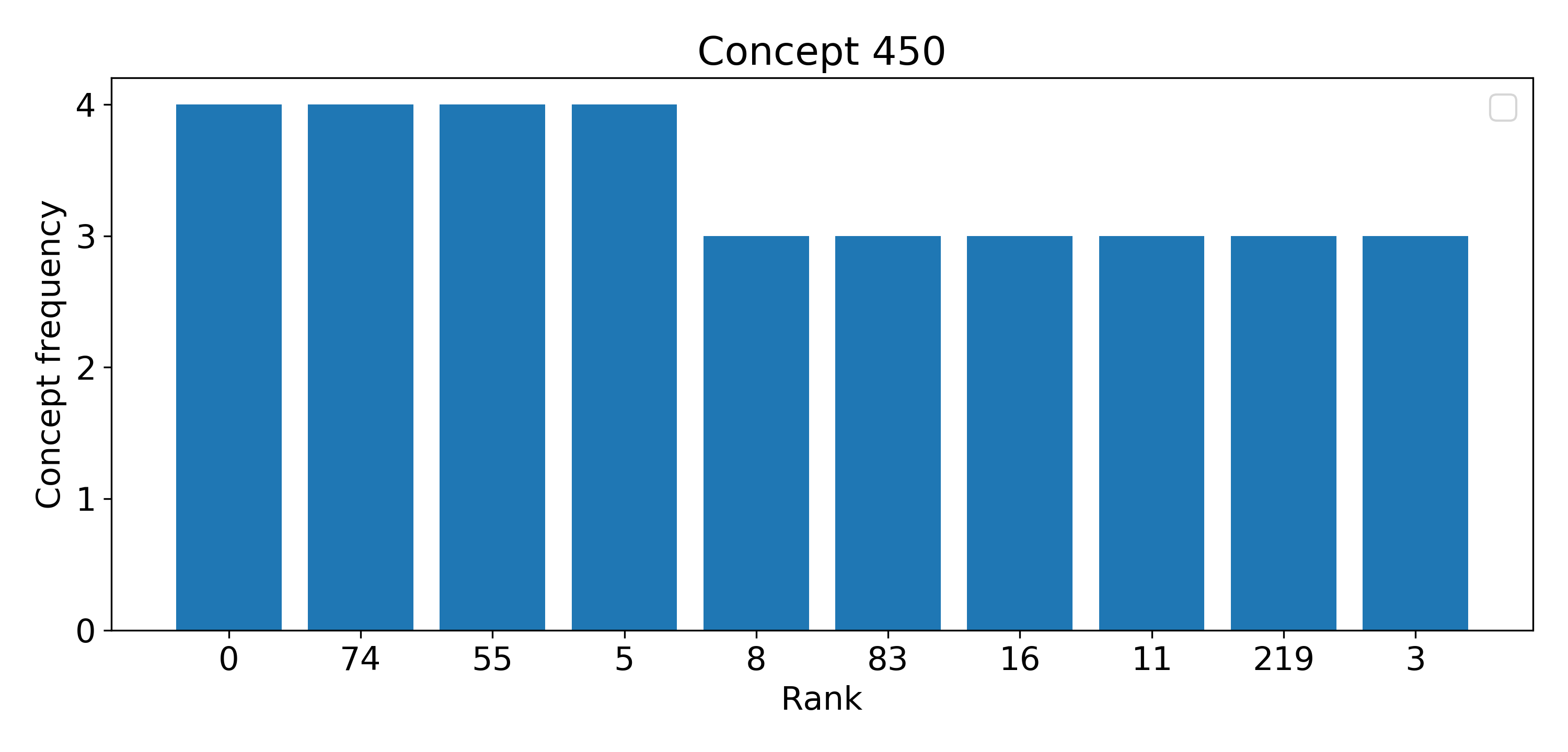
Figure 22: Ranks that are reached the most over all samples for the top-3 rule concepts for experiment ’Adience-Test-MF’. The 3 rules with the most covered samples (sample count in bold) are:
(144) Male, if concept 259 is above of concept 417
(48) Male, if concept 259 is above of concept 450
(25) Male, if concept 259 is below concept 417

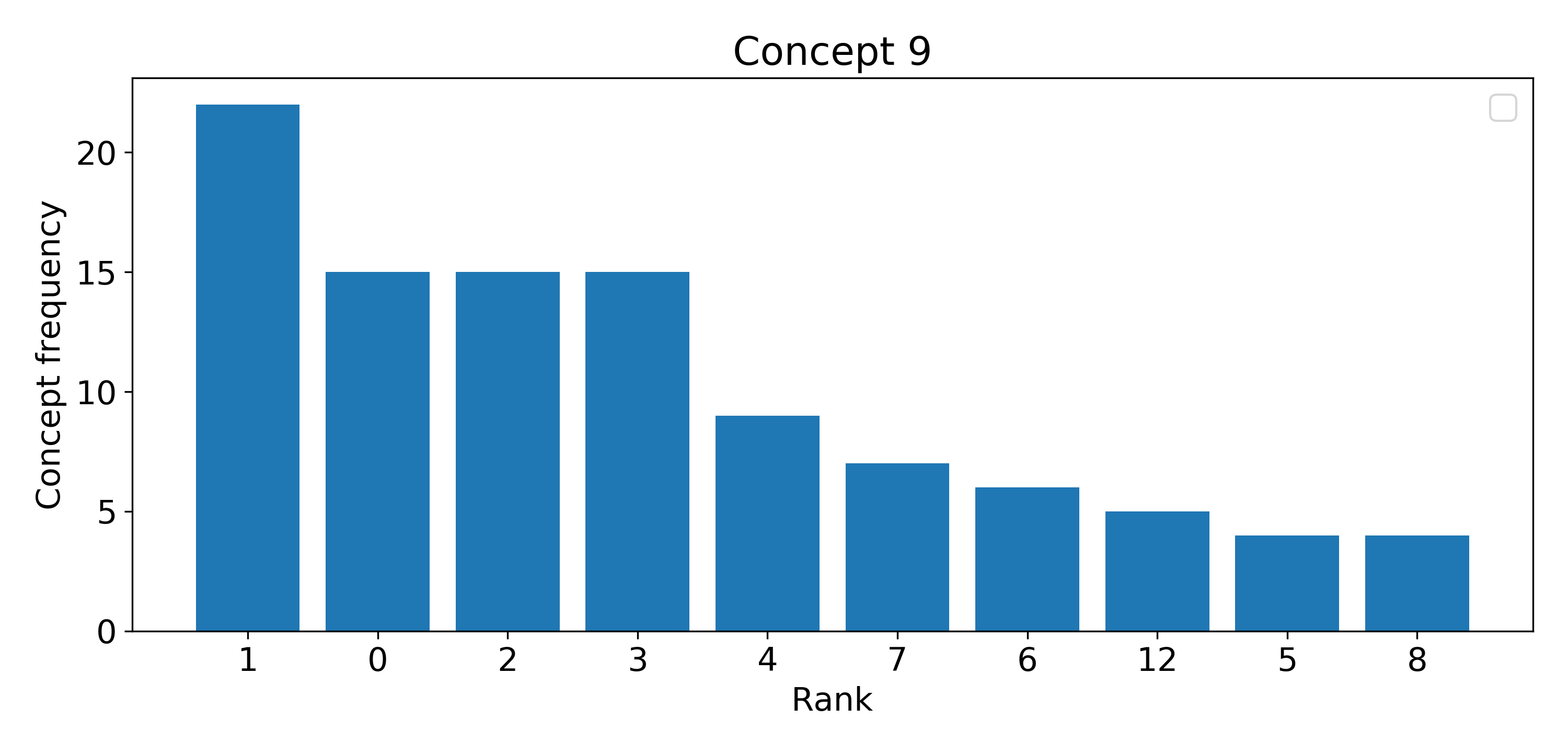
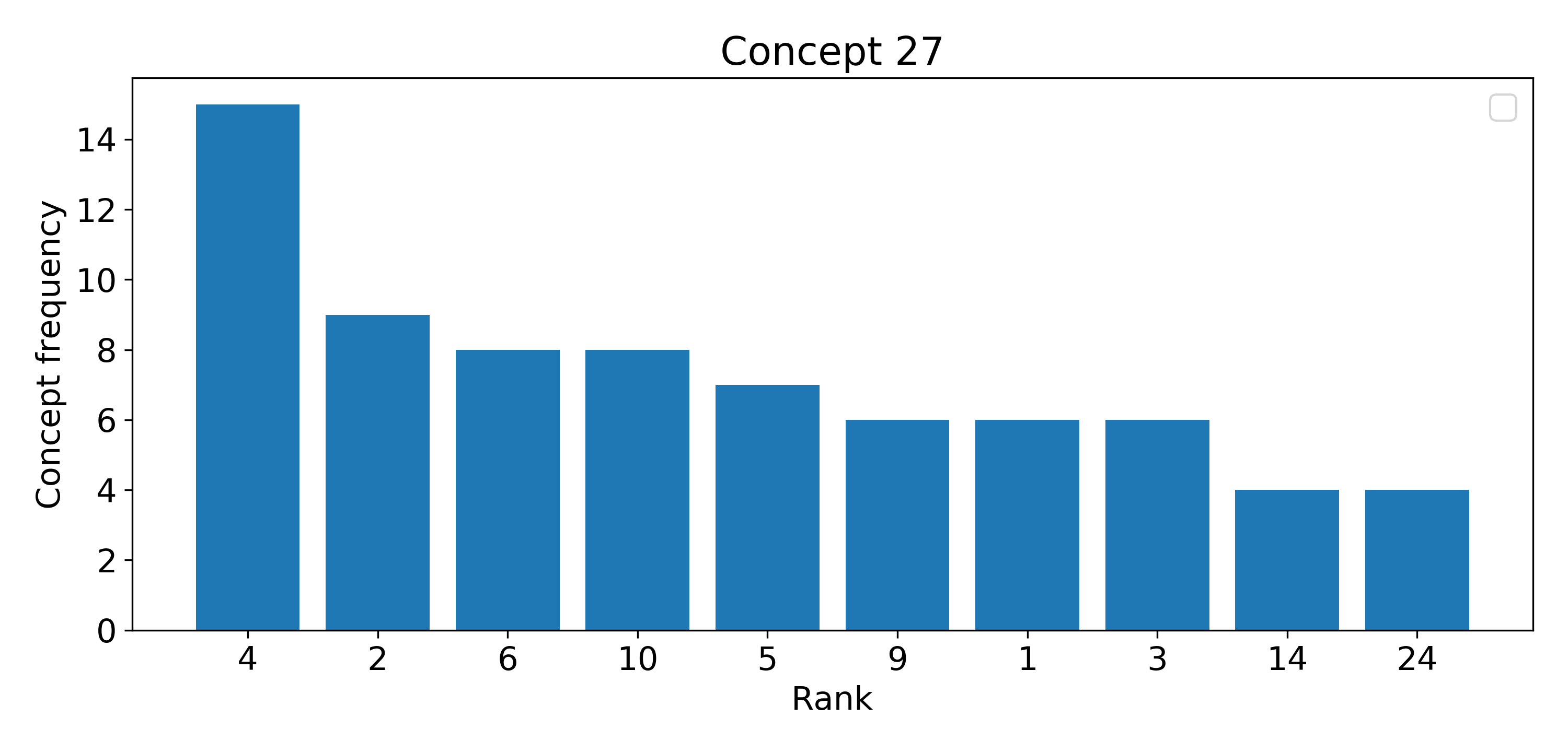
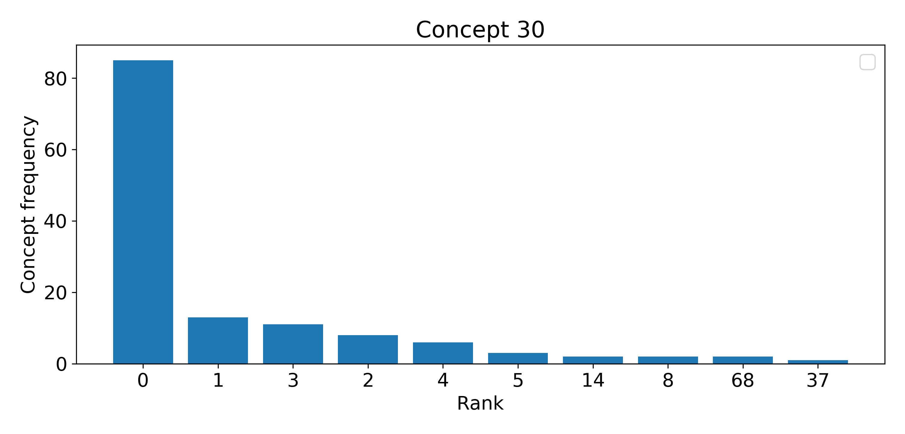
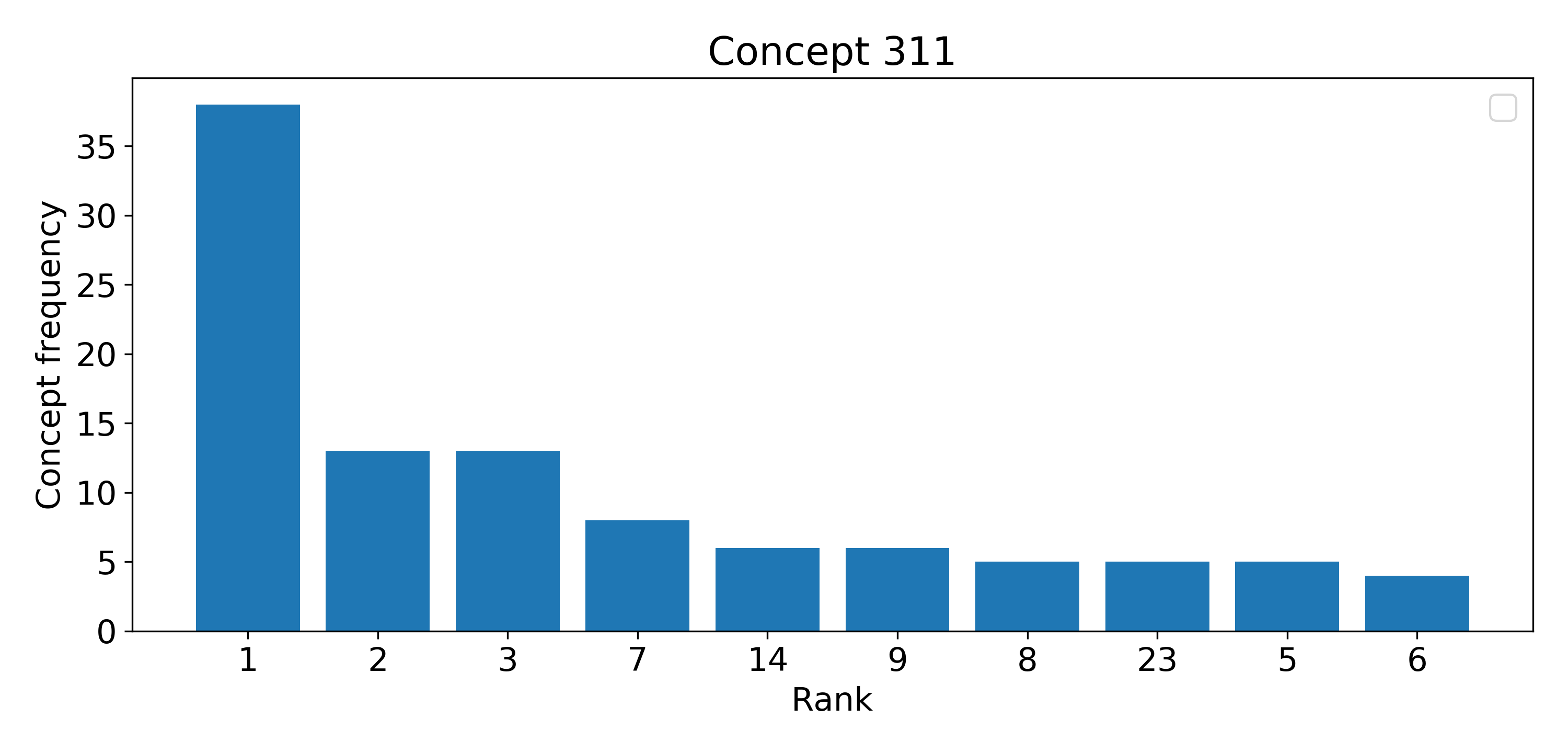
Figure 23: Ranks that are reached the most over all samples for the top-3 rule concepts for experiment ’Teapot-Vase-Train’. The 3 rules with the most covered samples (sample count in bold) are:
(97) Teapot, if concept 27 is above of concept 311
(89) Teapot, if concept 30 is middle right of concept 9
(52) Teapot, if concept 30 is right of concept 9

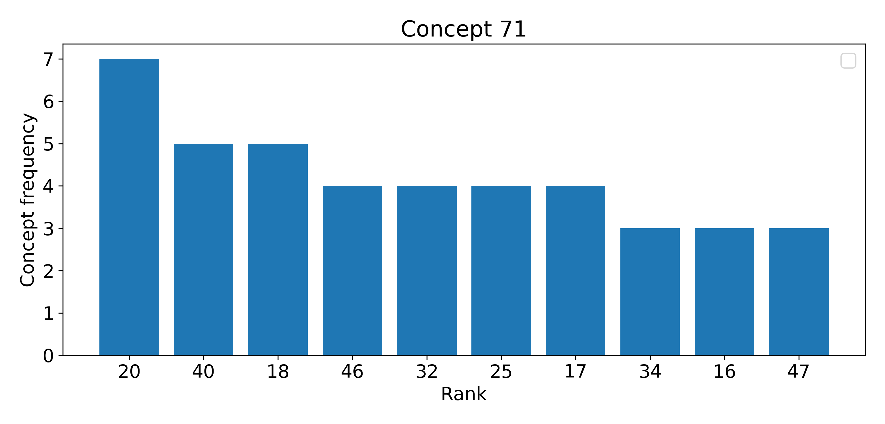
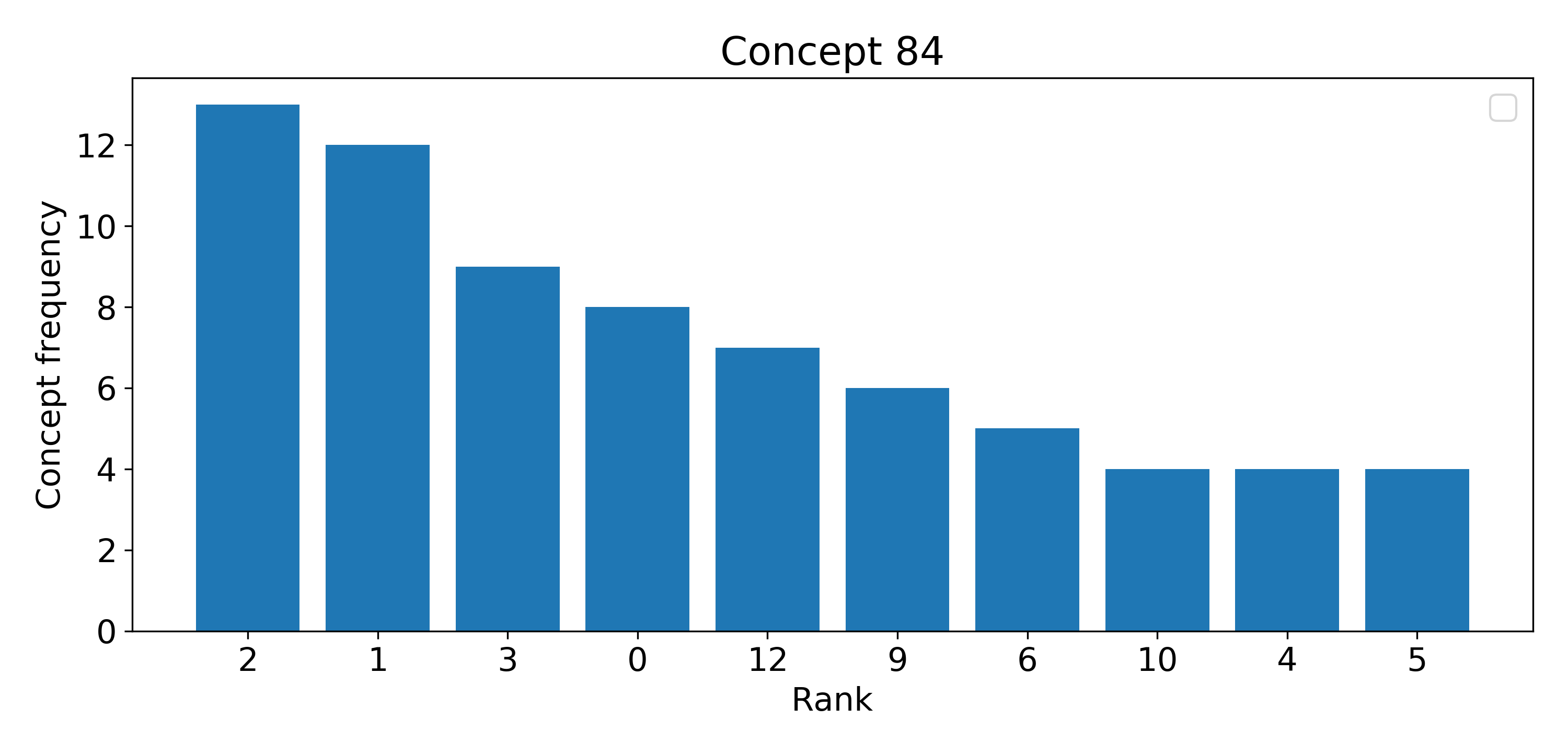
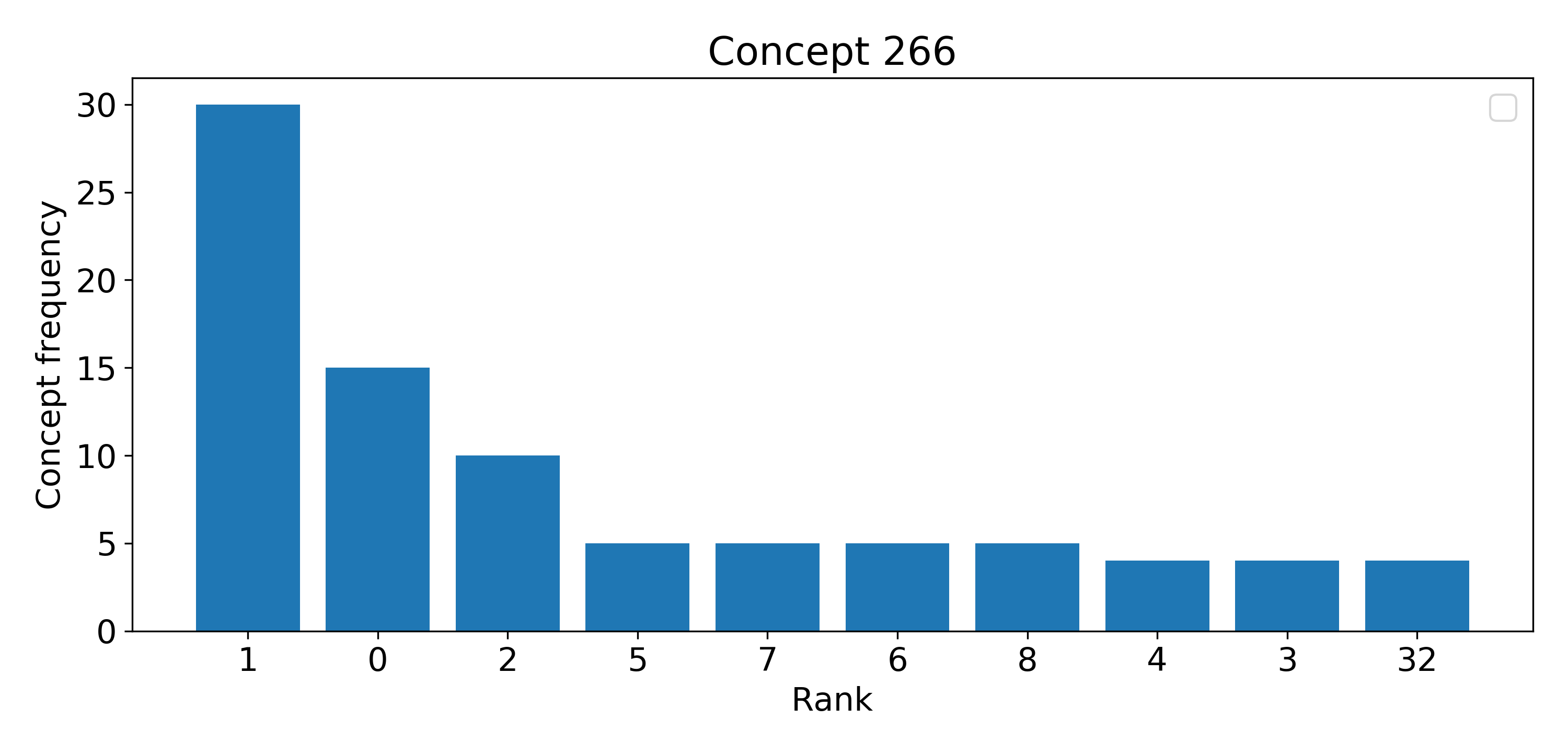
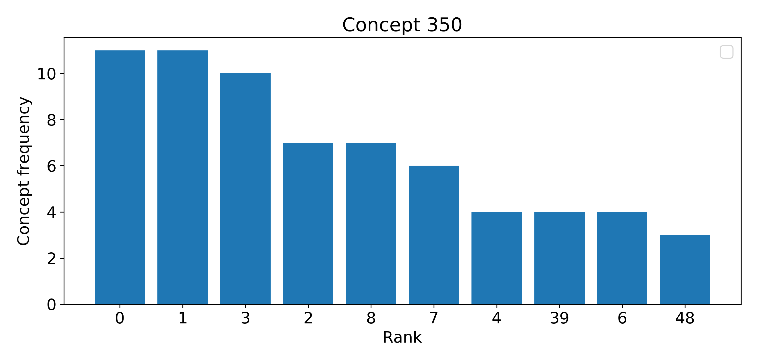
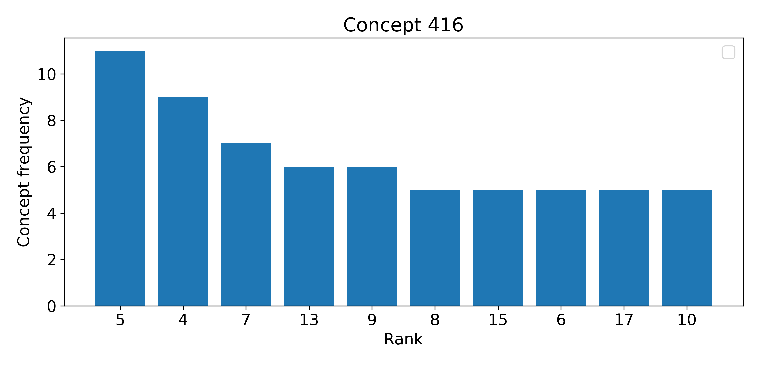
Figure 24: Ranks that are reached the most over all samples for the top-3 rule concepts for experiment ’Vase-Teapot-Train’. The 3 rules with the most covered samples (sample count in bold) are:
(70) Vase, if concept 350 is below concept 266
(66) Vase, if concept 71 is below concept 416
(49) Vase, if concept 84 is right of concept 3

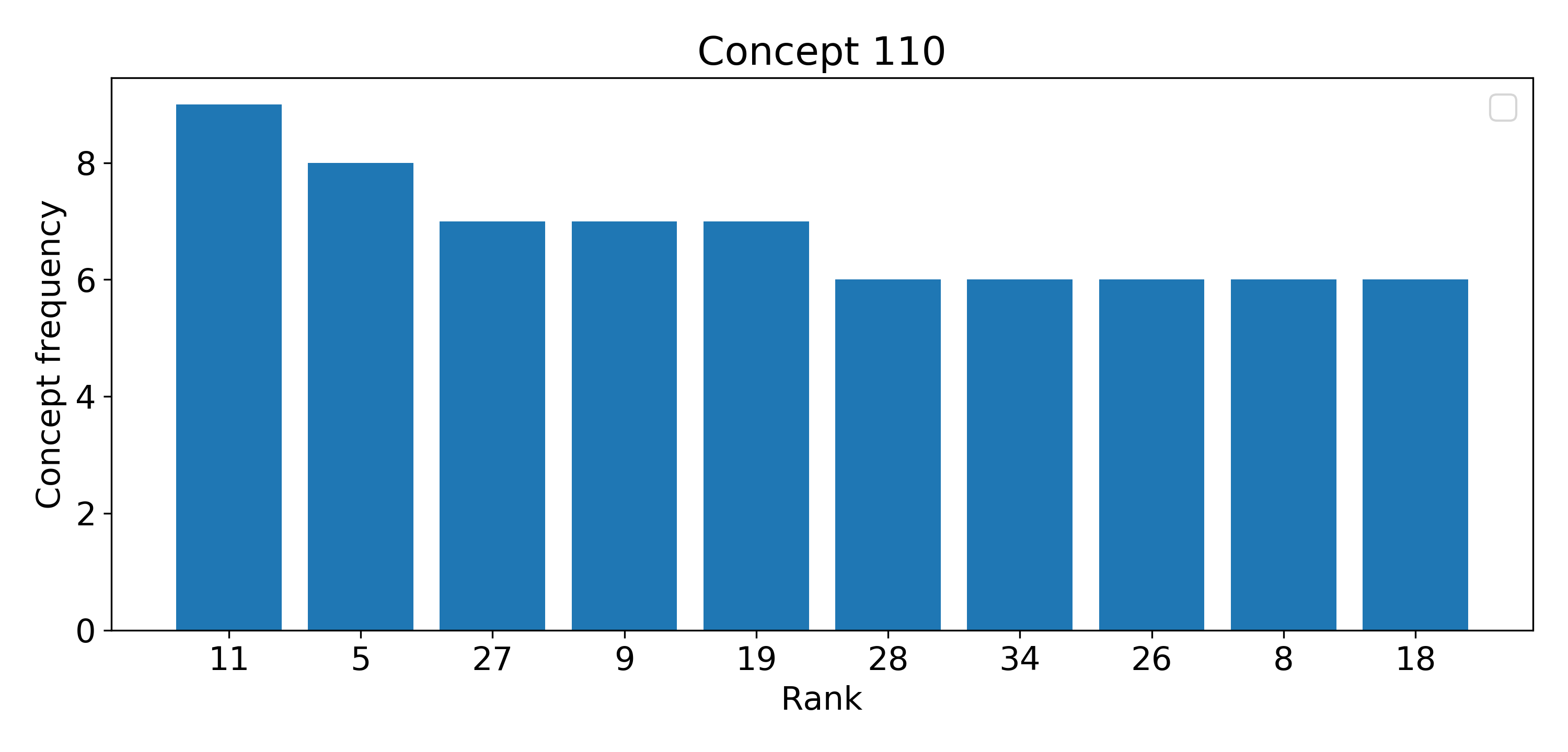
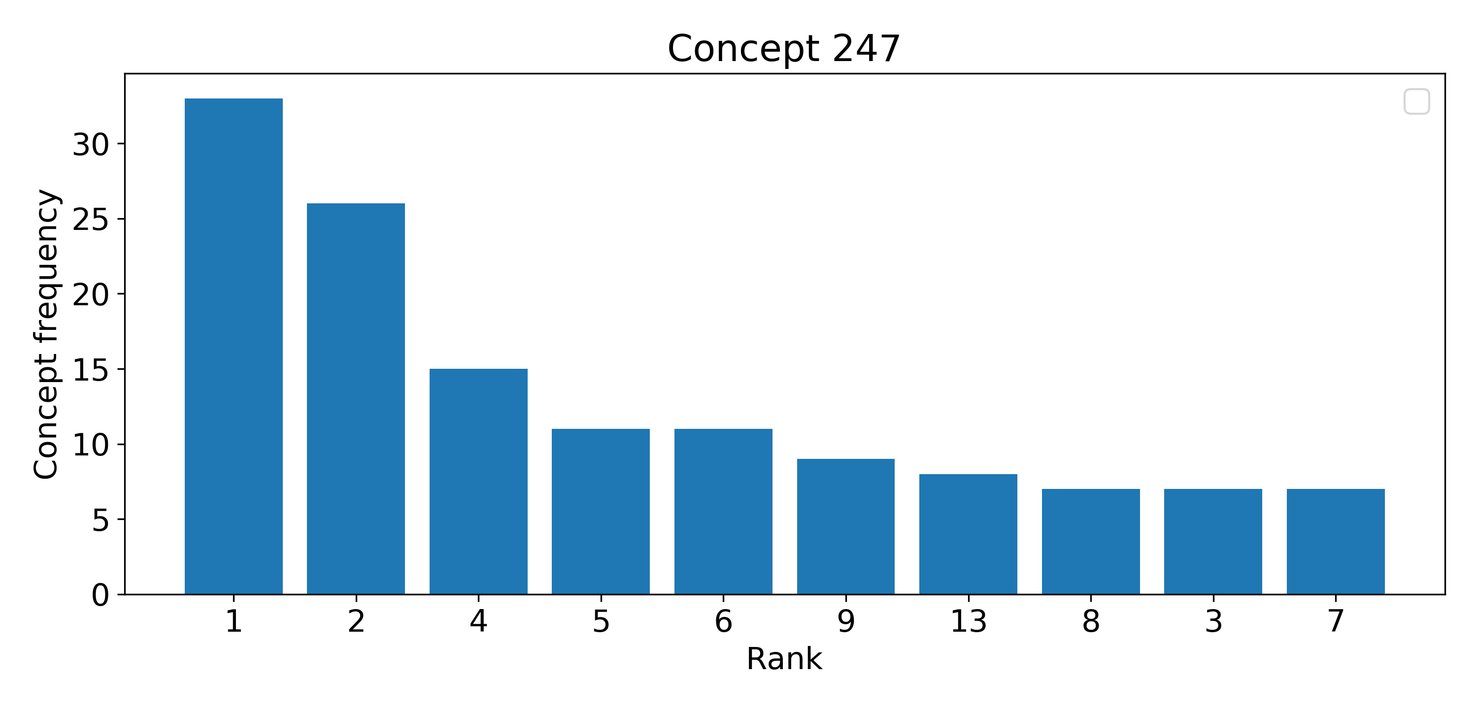
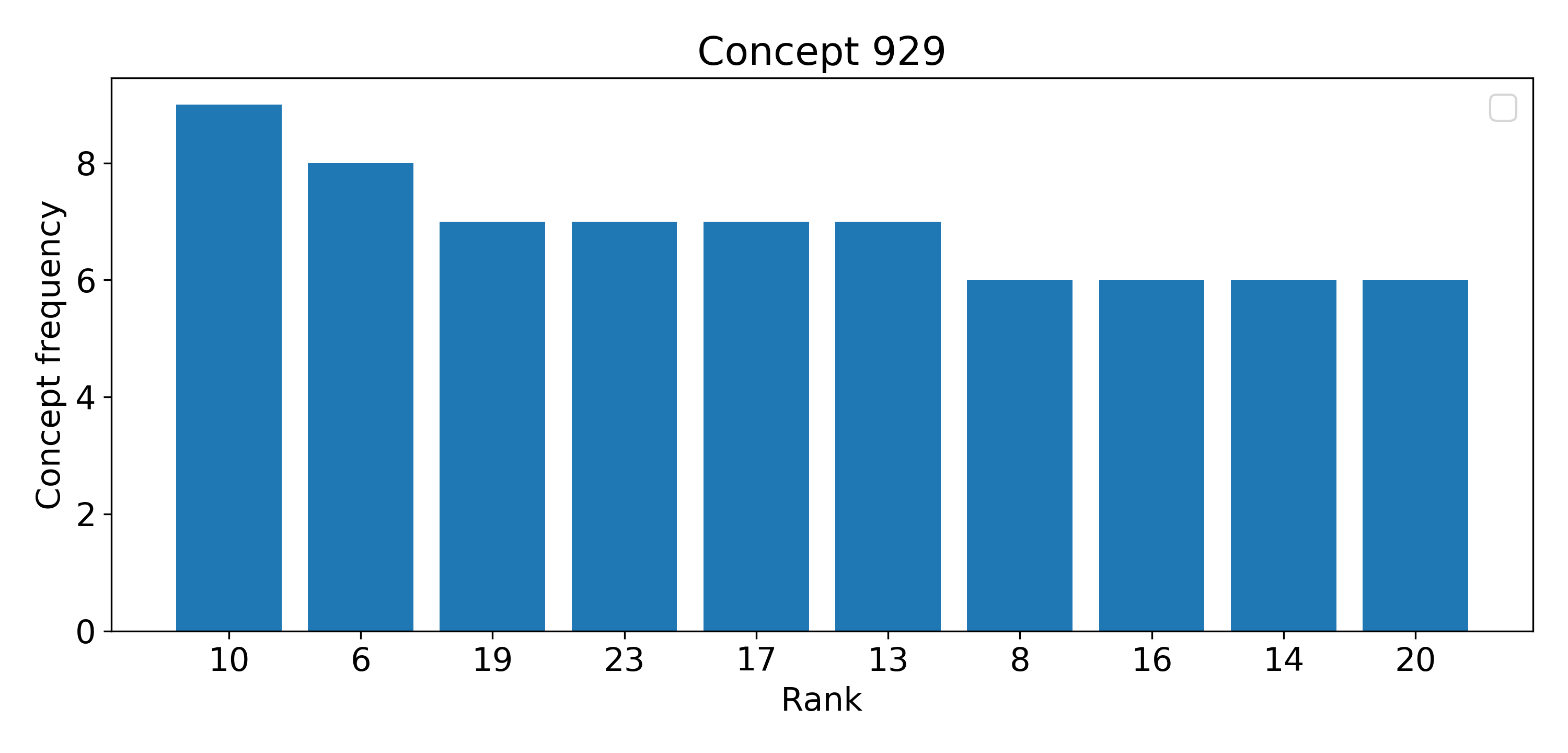
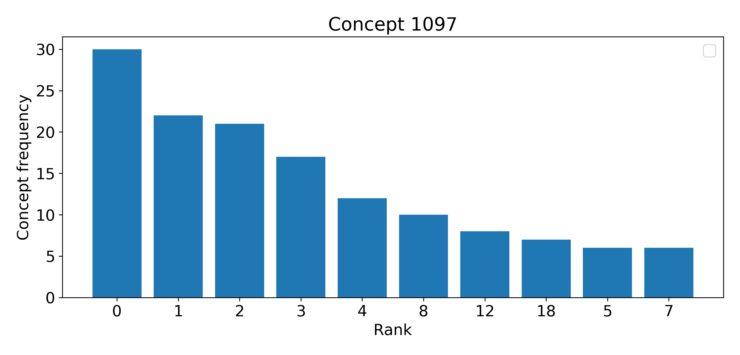
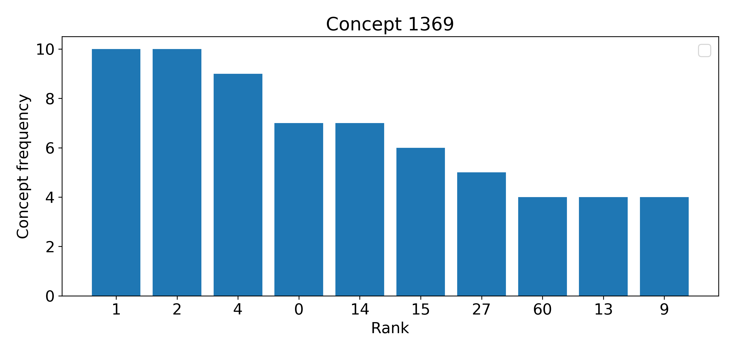
Figure 25: Ranks that are reached the most over all samples for the top-3 rule concepts for experiment ’PathMNIST-Train’. The 3 rules with the most covered samples (sample count in bold) are:
(213) Cancerous, if concept 1097 is bottom right of concept 247
(197) Cancerous, if sample contains concept 110
(115) Cancerous, if concept 1369 is middle right of concept 929

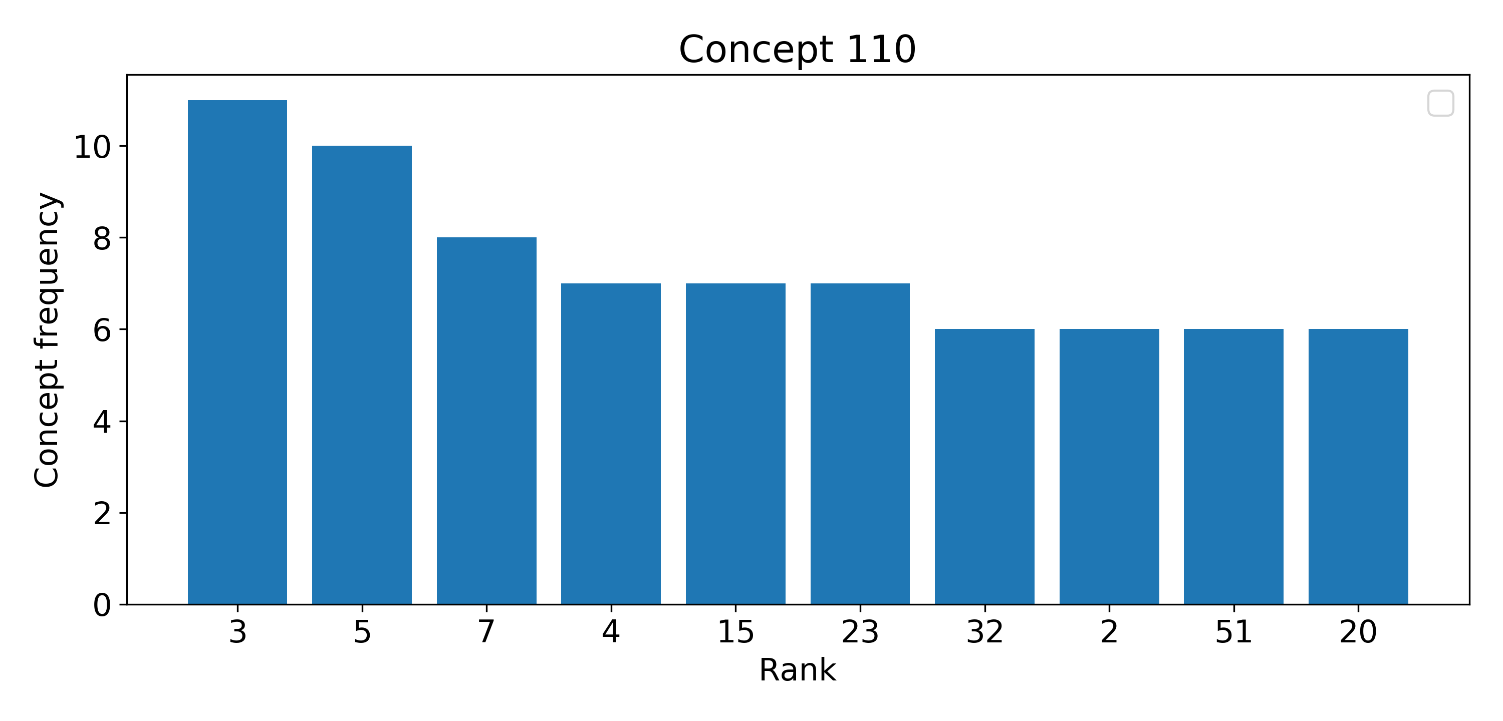
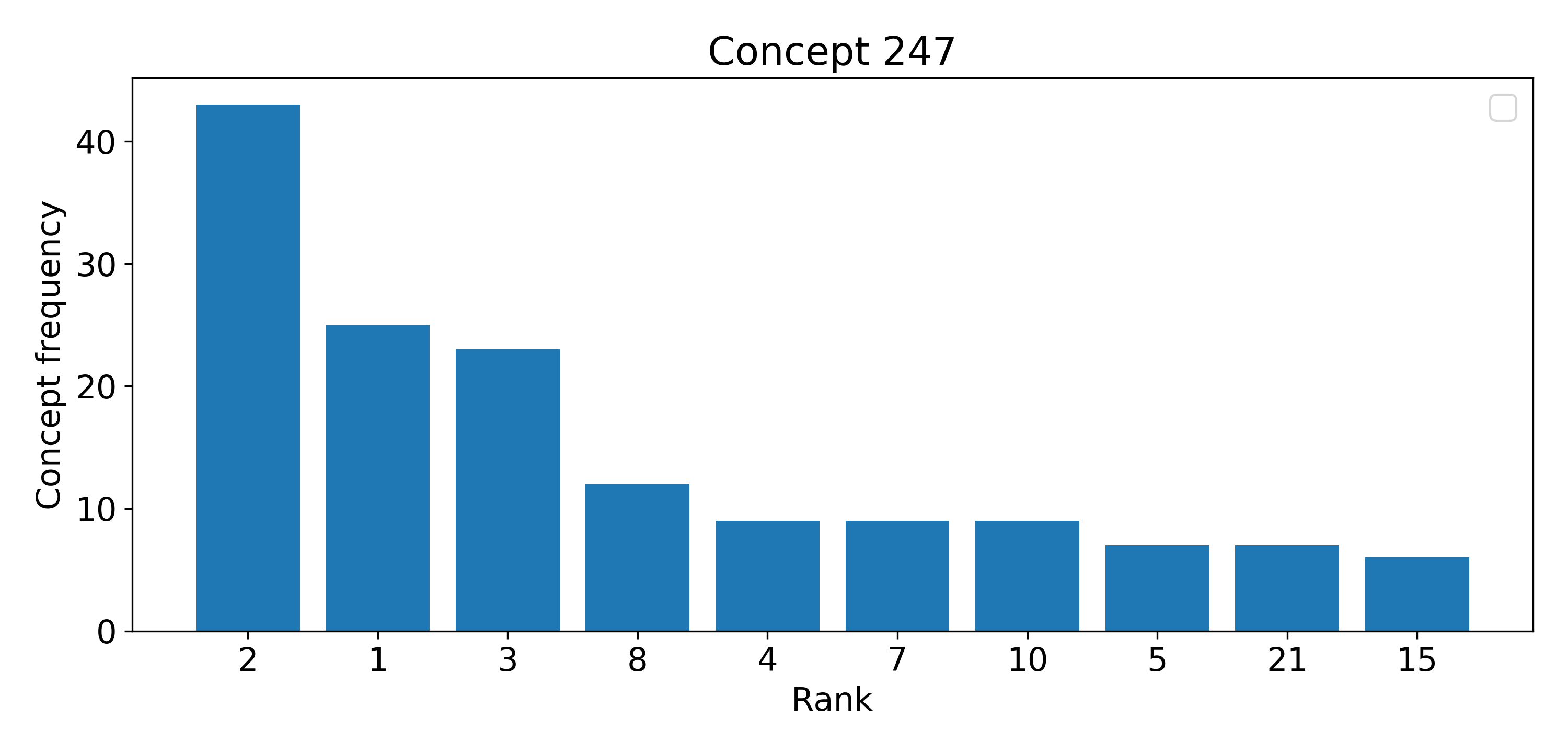
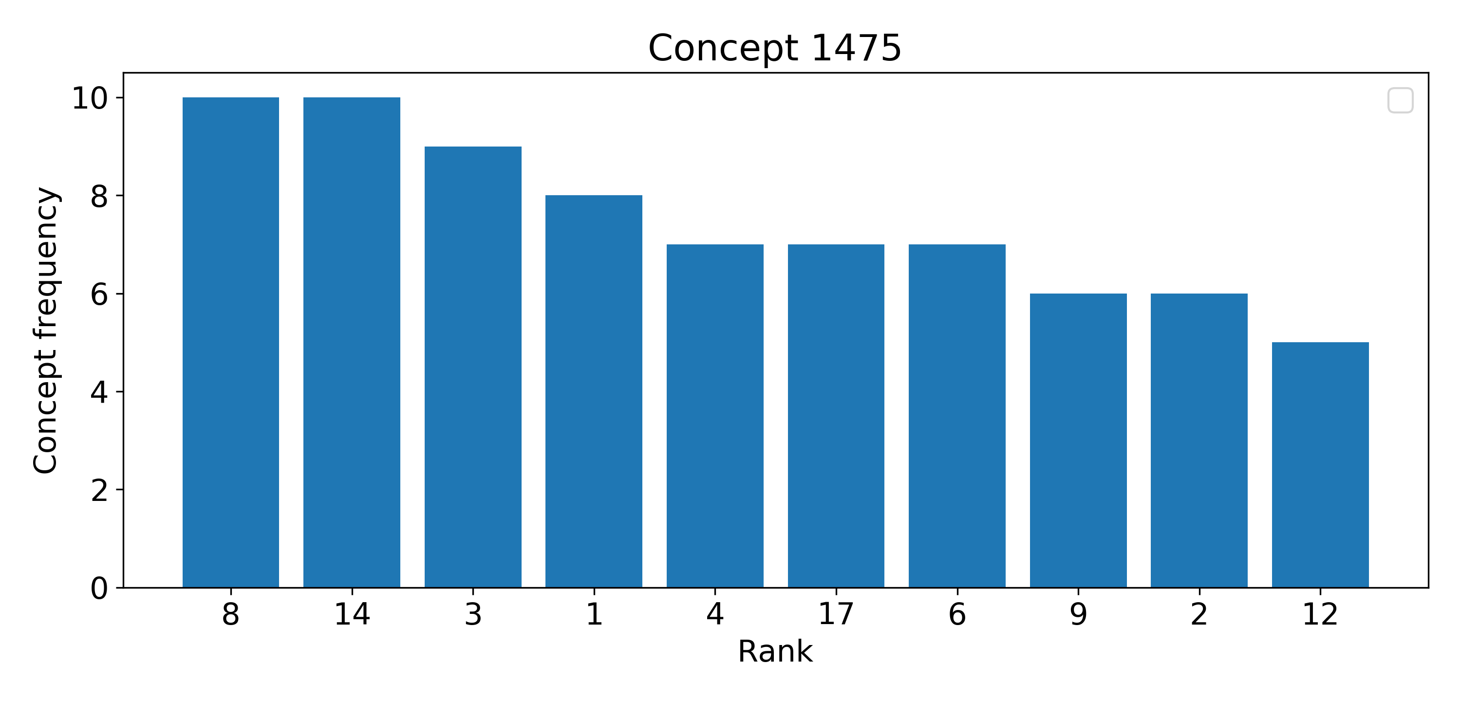
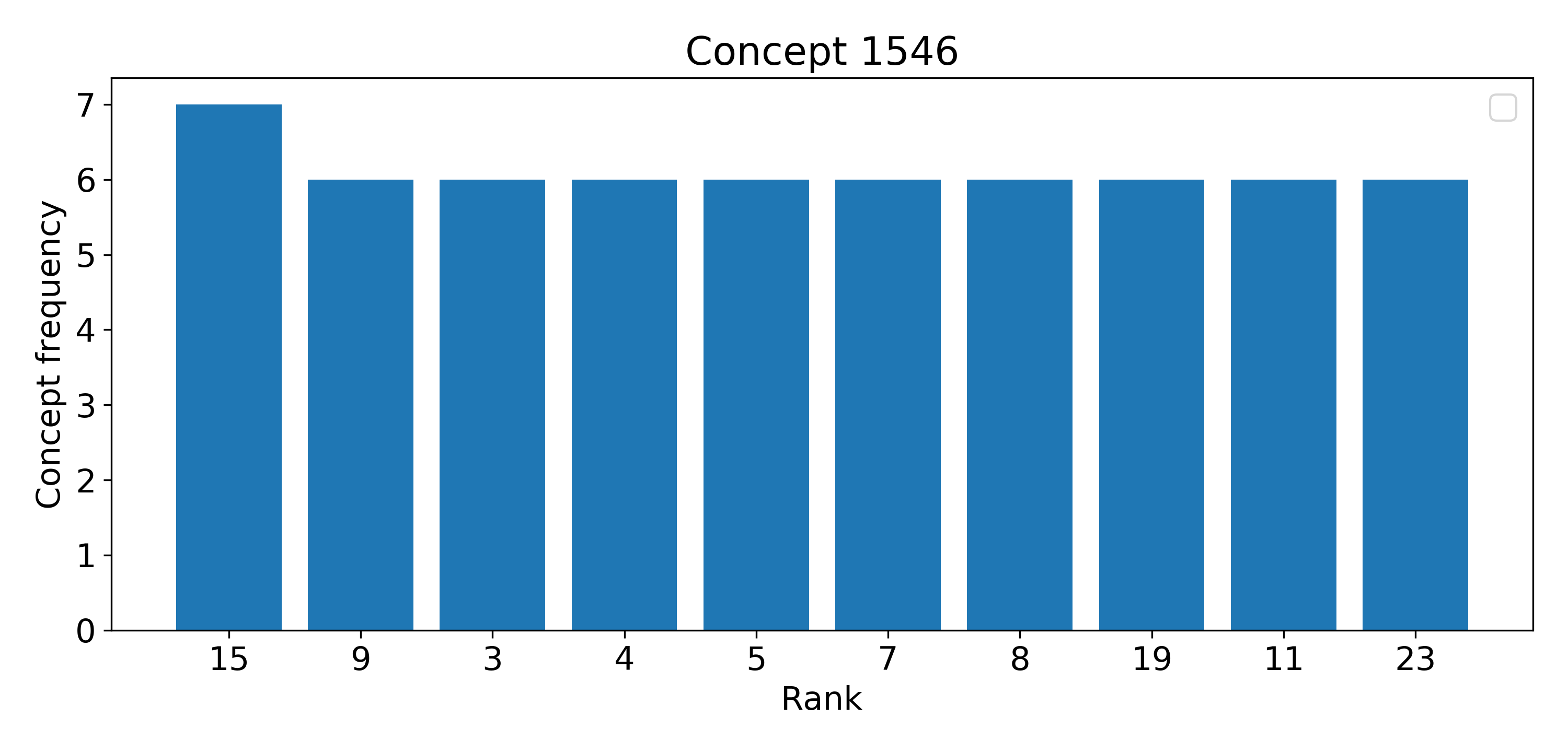
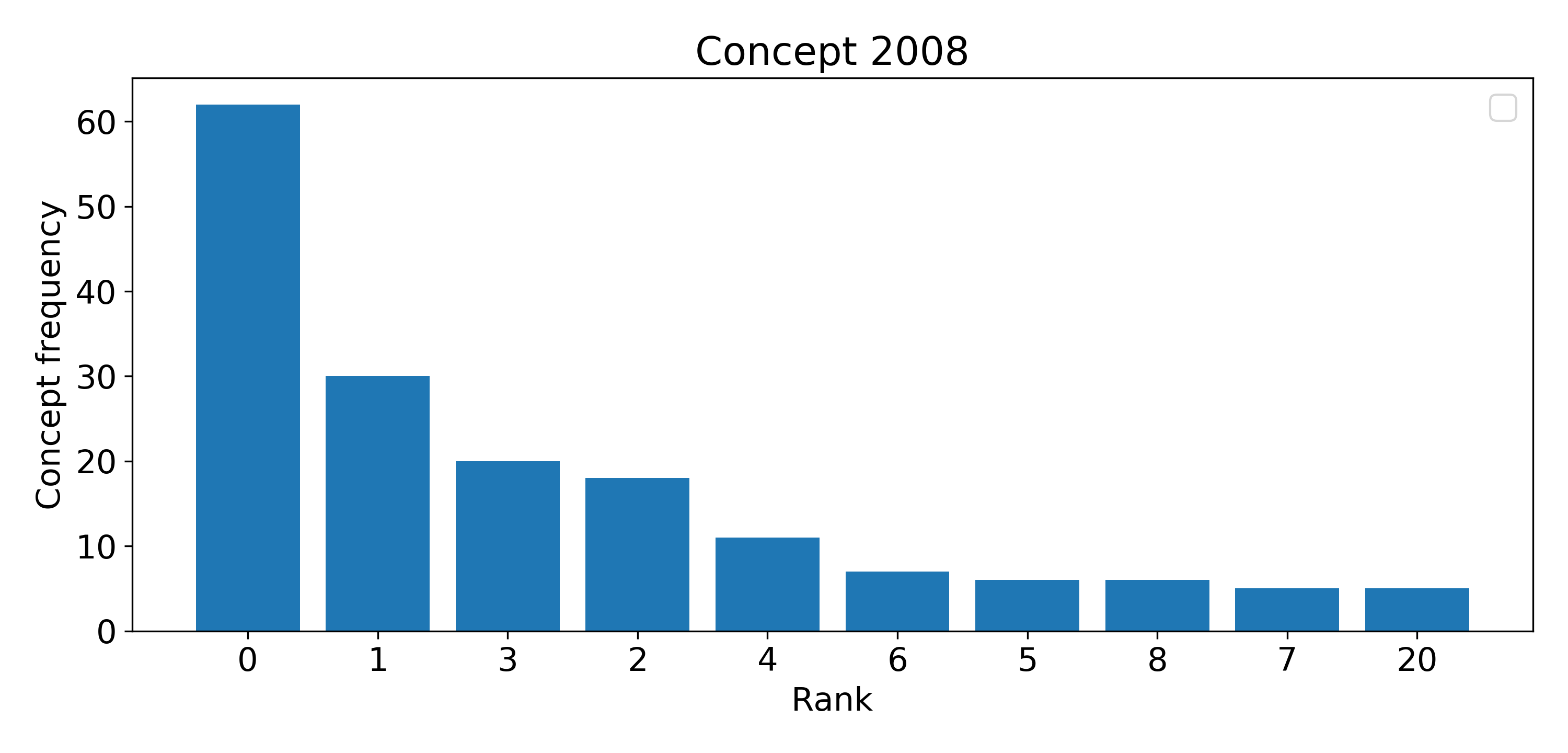
Figure 26: Ranks that are reached the most over all samples for the top-3 rule concepts for experiment ’PathMNIST-Test’. The 3 rules with the most covered samples (sample count in bold) are:
(208) Cancerous, if concept 247 is bottom middle of concept 2008
(191) Cancerous, if concept 110 is middle right of concept 2008
(166) Cancerous, if concept 1475 is middle right of concept 1546

References

- \bibcommenthead
- Achtibat et al (2022) Achtibat R, Dreyer M, Eisenbraun I, et al (2022) From ”where” to ”what”: Towards human-understandable explanations through concept relevance propagation. CoRR abs/2206.03208. 10.48550/arXiv.2206.03208, URL https://doi.org/10.48550/arXiv.2206.03208, https://arxiv.org/abs/2206.03208
- Achtibat et al (2023) Achtibat R, Dreyer M, Eisenbraun I, et al (2023) From attribution maps to human-understandable explanations through concept relevance propagation. Nat Mac Intell 5(9):1006–1019. 10.1038/S42256-023-00711-8, URL https://doi.org/10.1038/s42256-023-00711-8
- Adadi and Berrada (2018) Adadi A, Berrada M (2018) Peeking inside the black-box: A survey on explainable artificial intelligence (XAI). IEEE Access 6:52,138–52,160. 10.1109/ACCESS.2018.2870052, URL https://doi.org/10.1109/ACCESS.2018.2870052
- Arrieta et al (2020) Arrieta AB, Rodríguez ND, Ser JD, et al (2020) Explainable artificial intelligence (XAI): Concepts, taxonomies, opportunities and challenges toward responsible AI. Information Fusion 58:82–115. 10.1016/j.inffus.2019.12.012, URL https://doi.org/10.1016/j.inffus.2019.12.012
- Artelt and Hammer (2021) Artelt A, Hammer B (2021) Efficient computation of contrastive explanations. In: International Joint Conference on Neural Networks, IJCNN 2021, Shenzhen, China, July 18-22, 2021. IEEE, pp 1–9, 10.1109/IJCNN52387.2021.9534454, URL https://doi.org/10.1109/IJCNN52387.2021.9534454
- Bau et al (2017) Bau D, Zhou B, Khosla A, et al (2017) Network dissection: Quantifying interpretability of deep visual representations. In: 2017 IEEE Conference on Computer Vision and Pattern Recognition, CVPR 2017, Honolulu, HI, USA, July 21-26, 2017. IEEE Computer Society, pp 3319–3327, 10.1109/CVPR.2017.354, URL https://doi.org/10.1109/CVPR.2017.354
- Bontempelli et al (2023) Bontempelli A, Teso S, Tentori K, et al (2023) Concept-level debugging of part-prototype networks. In: The Eleventh International Conference on Learning Representations, ICLR 2023, Kigali, Rwanda, May 1-5, 2023. OpenReview.net, URL https://openreview.net/pdf?id=oiwXWPDTyNk
- Bruckert et al (2020) Bruckert S, Finzel B, Schmid U (2020) The next generation of medical decision support: A roadmap toward transparent expert companions. Frontiers in Artificial Intelligence 3:507,973. 10.3389/frai.2020.507973, URL https://doi.org/10.3389/frai.2020.507973
- Carvalho et al (2019) Carvalho DV, Pereira EM, Cardoso JS (2019) Machine learning interpretability: A survey on methods and metrics. Electronics 8(8):832. 10.3390/electronics8080832, URL https://www.mdpi.com/2079-9292/8/8/832
- Choi et al (2022) Choi H, Chang W, Choi J (2022) Can we find neurons that cause unrealistic images in deep generative networks? In: Raedt LD (ed) Proc. of the 31st IJCAI. ijcai.org, pp 2888–2894, 10.24963/ijcai.2022/400, URL https://doi.org/10.24963/ijcai.2022/400
- Clementini and Felice (1996) Clementini E, Felice PD (1996) A model for representing topological relationships between complex geometric features in spatial databases. Information Science 90(1-4):121–136. 10.1016/0020-0255(95)00289-8, URL https://doi.org/10.1016/0020-0255(95)00289-8
- Clementini et al (1993) Clementini E, Felice PD, van Oosterom P (1993) A small set of formal topological relationships suitable for end-user interaction. In: Abel DJ, Ooi BC (eds) Advances in Spatial Databases, Third International Symposium, SSD’93, Singapore, June 23-25, 1993, Proceedings, Lecture Notes in Computer Science, vol 692. Springer, pp 277–295, 10.1007/3-540-56869-7_16, URL https://doi.org/10.1007/3-540-56869-7_16
- Dash et al (2022) Dash T, Chitlangia S, Ahuja A, et al (2022) A review of some techniques for inclusion of domain-knowledge into deep neural networks. Scientific Reports 12(1):1040. 10.1038/s41598-021-04590-0, URL https://doi.org/10.1038/s41598-021-04590-0
- Deng et al (2009) Deng J, Dong W, Socher R, et al (2009) Imagenet: A large-scale hierarchical image database. In: 2009 IEEE Computer Society Conference on Computer Vision and Pattern Recognition (CVPR 2009), 20-25 June 2009, Miami, Florida, USA. IEEE Computer Society, pp 248–255, 10.1109/CVPR.2009.5206848, URL https://doi.org/10.1109/CVPR.2009.5206848
- Du et al (2020) Du M, Liu N, Hu X (2020) Techniques for interpretable machine learning. Commun ACM 63(1):68–77. 10.1145/3359786, URL https://doi.org/10.1145/3359786
- Eidinger et al (2014) Eidinger E, Enbar R, Hassner T (2014) Age and gender estimation of unfiltered faces. IEEE Transactions on Information Forensics and Security 9(12):2170–2179. 10.1109/TIFS.2014.2359646, URL https://doi.org/10.1109/TIFS.2014.2359646
- Finzel (2024) Finzel B (2024) Human-centered explanations: Lessons learned from image classification for medical and clinical decision making. KI-Künstliche Intelligenz 10.1007/s13218-024-00835-y, URL https://doi.org/10.1007/s13218-024-00835-y
- Finzel et al (2024) Finzel B, Kuhn SP, Tafler DE, et al (2024) Explaining with attribute-based and relational near misses: An interpretable approach to distinguishing facial expressions of pain and disgust. In: Muggleton SH, Tamaddoni-Nezhad A (eds) Inductive Logic Programming. Springer Nature Switzerland, Cham, pp 40–51, https://doi.org/10.1007/978-3-031-55630-2_4
- Fong and Vedaldi (2018) Fong R, Vedaldi A (2018) Net2vec: Quantifying and explaining how concepts are encoded by filters in deep neural networks. In: 2018 IEEE Conference on Computer Vision and Pattern Recognition, CVPR 2018, Salt Lake City, UT, USA, June 18-22, 2018. Computer Vision Foundation / IEEE Computer Society, pp 8730–8738, 10.1109/CVPR.2018.00910, URL http://openaccess.thecvf.com/content_cvpr_2018/html/Fong_Net2Vec_Quantifying_and_CVPR_2018_paper.html
- Gillies (2022) Gillies S (2022) Shapely documentation. Tech. rep., https://shapely.readthedocs.io/_/downloads/en/1.8.1/pdf/
- Guidotti et al (2019) Guidotti R, Monreale A, Ruggieri S, et al (2019) A survey of methods for explaining black box models. ACM Comput Surv 51(5):93:1–93:42. 10.1145/3236009, URL https://doi.org/10.1145/3236009
- He et al (2016) He K, Zhang X, Ren S, et al (2016) Deep residual learning for image recognition. In: 2016 IEEE Conference on Computer Vision and Pattern Recognition, CVPR 2016, Las Vegas, NV, USA, June 27-30, 2016. IEEE Computer Society, pp 770–778, 10.1109/CVPR.2016.90, URL https://doi.org/10.1109/CVPR.2016.90
- Herchenbach et al (2022) Herchenbach M, Müller D, Scheele S, et al (2022) Explaining image classifications with near misses, near hits and prototypes - supporting domain experts in understanding decision boundaries. In: El-Yacoubi MA, Granger E, Yuen PC, et al (eds) Pattern Recognition and Artificial Intelligence - Third International Conference, ICPRAI 2022, Paris, France, June 1-3, 2022, Proceedings, Part II, Lecture Notes in Computer Science, vol 13364. Springer, pp 419–430, 10.1007/978-3-031-09282-4_35, URL https://doi.org/10.1007/978-3-031-09282-4_35
- Kather et al (2019) Kather JN, Krisam J, Charoentong P, et al (2019) Predicting survival from colorectal cancer histology slides using deep learning: A retrospective multicenter study. PLoS Medicine 16(1):e1002,730. https://doi.org/10.1371/journal.pmed.1002730
- Khan et al (2015) Khan K, Mauro M, Leonardi R (2015) Multi-class semantic segmentation of faces. In: 2015 IEEE International Conference on Image Processing, ICIP 2015, Quebec City, QC, Canada, September 27-30, 2015. IEEE, pp 827–831, 10.1109/ICIP.2015.7350915, URL https://doi.org/10.1109/ICIP.2015.7350915
- Kim et al (2016) Kim B, Koyejo O, Khanna R (2016) Examples are not enough, learn to criticize! criticism for interpretability. In: Lee DD, Sugiyama M, von Luxburg U, et al (eds) Advances in Neural Information Processing Systems 29: Annual Conference on Neural Information Processing Systems 2016, December 5-10, 2016, Barcelona, Spain, pp 2280–2288, URL https://proceedings.neurips.cc/paper/2016/hash/5680522b8e2bb01943234bce7bf84534-Abstract.html
- Lapuschkin (2019) Lapuschkin S (2019) Opening the machine learning black box with layer-wise relevance propagation. PhD thesis, Technical University of Berlin, Germany, URL https://nbn-resolving.org/urn:nbn:de:101:1-2019020600591967118475
- Lapuschkin et al (2019) Lapuschkin S, Wäldchen S, Binder A, et al (2019) Unmasking clever hans predictors and assessing what machines really learn. Nature Communications 10(1):1–8
- Manhaeve et al (2021) Manhaeve R, Dumancic S, Kimmig A, et al (2021) Neural probabilistic logic programming in deepproblog. Artif Intell 298:103,504. 10.1016/J.ARTINT.2021.103504, URL https://doi.org/10.1016/j.artint.2021.103504
- McKee et al (2014) McKee JL, Riesenhuber M, Miller EK, et al (2014) Task dependence of visual and category representations in prefrontal and inferior temporal cortices. Journal of Neuroscience 34(48):16,065–16,075
- Miller and Johnson-Laird (2013) Miller G, Johnson-Laird P (2013) Language and Perception. Harvard University Press, URL https://books.google.de/books?id=bi0YnwEACAAJ
- Miller (2021) Miller T (2021) Contrastive explanation: a structural-model approach. Knowl Eng Rev 36:e14. 10.1017/S0269888921000102, URL https://doi.org/10.1017/S0269888921000102
- Mitchell (1997) Mitchell TM (1997) Machine Learning. McGraw-Hill
- Montavon et al (2019) Montavon G, Binder A, Lapuschkin S, et al (2019) Layer-wise relevance propagation: An overview. In: Explainable AI: Interpreting, Explaining and Visualizing Deep Learning, Lecture Notes in Computer Science, vol 11700. Springer, p 193–209, 10.1007/978-3-030-28954-6_10, URL https://doi.org/10.1007/978-3-030-28954-6_10
- Muggleton (1991) Muggleton SH (1991) Inductive logic programming. New Generation Computing 8(4):295–318. 10.1007/BF03037089, URL https://doi.org/10.1007/BF03037089
- Muggleton et al (2018) Muggleton SH, Schmid U, Zeller C, et al (2018) Ultra-strong machine learning: comprehensibility of programs learned with ILP. Mach Learn 107(7):1119–1140. 10.1007/S10994-018-5707-3, URL https://doi.org/10.1007/s10994-018-5707-3
- Poeta et al (2023) Poeta E, Ciravegna G, Pastor E, et al (2023) Concept-based explainable artificial intelligence: A survey. arXiv preprint arXiv:231212936
- Rabold et al (2019) Rabold J, Deininger H, Siebers M, et al (2019) Enriching visual with verbal explanations for relational concepts - Combining LIME with Aleph. In: Proc. of the ECML PKDD, Communications in Computer and Information Science, vol 1167. Springer, pp 180–192, 10.1007/978-3-030-43823-4_16, URL https://doi.org/10.1007/978-3-030-43823-4_16
- Rabold et al (2020) Rabold J, Schwalbe G, Schmid U (2020) Expressive explanations of DNNs by combining concept analysis with ILP. In: German Conference on Artificial Intelligence (Künstliche Intelligenz), Springer, pp 148–162
- Rabold et al (2022) Rabold J, Siebers M, Schmid U (2022) Generating contrastive explanations for inductive logic programming based on a near miss approach. Machine Learning 111(5):1799–1820. 10.1007/s10994-021-06048-w, URL https://doi.org/10.1007/s10994-021-06048-w
- Renz (2002) Renz J (2002) Qualitative spatial reasoning with topological information. Springer
- Ribeiro et al (2016) Ribeiro MT, Singh S, Guestrin C (2016) ”Why should I trust you?”: Explaining the predictions of any classifier. In: Proc. of the 22nd ACM SIGKDD. ACM, pp 1135–1144, 10.1145/2939672.2939778, URL https://doi.org/10.1145/2939672.2939778
- Rosch (1973) Rosch EH (1973) Natural categories. Cognitive Psychology 4(3):328–350
- Schramowski et al (2020) Schramowski P, Stammer W, Teso S, et al (2020) Making deep neural networks right for the right scientific reasons by interacting with their explanations. Nat Mach Intell 2(8):476–486. 10.1038/S42256-020-0212-3, URL https://doi.org/10.1038/s42256-020-0212-3
- Schwalbe and Finzel (2023) Schwalbe G, Finzel B (2023) A comprehensive taxonomy for explainable artificial intelligence: A systematic survey of surveys on methods and concepts. Data Mining and Knowledge Discovery pp 1–59
- Simons (2000) Simons P (2000) Parts: A Study in Ontology. Oxford University Press
- Simonyan and Zisserman (2015) Simonyan K, Zisserman A (2015) Very deep convolutional networks for large-scale image recognition. In: Proc. of the 3rd ICLR, URL http://arxiv.org/abs/1409.1556
- Smith and Medin (2013) Smith EE, Medin DL (2013) Categories and concepts. Harvard University Press
- Sriharee (2015) Sriharee G (2015) A symbolic-based indoor navigation system with direction-based navigation instruction. In: Shakshuki EM (ed) Proceedings of the 6th International Conference on Ambient Systems, Networks and Technologies (ANT 2015), the 5th International Conference on Sustainable Energy Information Technology (SEIT-2015), London, UK, June 2-5, 2015, Procedia Computer Science, vol 52. Elsevier, pp 647–653, 10.1016/j.procs.2015.05.065, URL https://doi.org/10.1016/j.procs.2015.05.065
- Srinivasan (2007) Srinivasan A (2007) The Aleph Manual. URL https://www.cs.ox.ac.uk/activities/programinduction/Aleph/aleph.html
- Srinivasan et al (2019) Srinivasan A, Vig L, Bain M (2019) Logical explanations for deep relational machines using relevance information. J Mach Learn Res 20:130:1–130:47. URL http://jmlr.org/papers/v20/18-517.html
- Stammer et al (2021) Stammer W, Schramowski P, Kersting K (2021) Right for the right concept: Revising neuro-symbolic concepts by interacting with their explanations. In: Proc. of the IEEE CVPR. IEEE Computer Society, pp 3619–3629, 10.1109/CVPR46437.2021.00362, URL https://openaccess.thecvf.com/content/CVPR2021/html/Stammer_Right_for_the_Right_Concept_Revising_Neuro-Symbolic_Concepts_by_Interacting_CVPR_2021_paper.html
- Teso and Kersting (2019) Teso S, Kersting K (2019) Explanatory interactive machine learning. In: Proc. of the AAAI/ACM AIES. ACM, pp 239–245, 10.1145/3306618.3314293, URL https://doi.org/10.1145/3306618.3314293
- Teso et al (2022) Teso S, Alkan Ö, Stammer W, et al (2022) Leveraging explanations in interactive machine learning: An overview. CoRR abs/2207.14526. 10.48550/arXiv.2207.14526, URL https://doi.org/10.48550/arXiv.2207.14526, https://arxiv.org/abs/2207.14526
- Wille (2005) Wille R (2005) Formal concept analysis as mathematical theory of concepts and concept hierarchies. In: Formal Concept Analysis. Springer, p 1–33
- Yang et al (2021) Yang J, Shi R, Wei D, et al (2021) MedMNIST v2: A large-scale lightweight benchmark for 2d and 3d biomedical image classification. CoRR abs/2110.14795. URL https://arxiv.org/abs/2110.14795, https://arxiv.org/abs/2110.14795