Confidence regions for a persistence diagram of a single image with one or more loops

Abstract

Topological data analysis (TDA) uses persistent homology to quantify loops and higher-dimensional holes in data, making it particularly relevant for examining the characteristics of images of cells in the field of cell biology. In the context of a cell injury, as time progresses, a wound in the form of a ring emerges in the cell image and then gradually vanishes. Performing statistical inference on this ring-like pattern in a single image is challenging due to the absence of repeated samples. In this paper, we develop a novel framework leveraging TDA to estimate underlying structures within individual images and quantify associated uncertainties through confidence regions. Our proposed method partitions the image into the background and the damaged cell regions. Then pixels within the affected cell region are used to establish confidence regions in the space of persistence diagrams (topological summary statistics). The method establishes estimates on the persistence diagrams which correct the bias of traditional TDA approaches. A simulation study is conducted to evaluate the coverage probabilities of the proposed confidence regions in comparison to an alternative approach is proposed in this paper. We also illustrate our methodology by a real-world example provided by cell repair.

Keywords: Bootstrapping, Confidence Regions, Image Processing, Pattern detection, Topological Data Analysis, Uncertainty Quantification

1 Introduction

Ring-like patterns are ubiquitous in biology, being evident during cell division (Pollard and O’Shaughnessy, 2019), development (Haglund et al., 2019), and the response of immune cells to challenges (Herron et al., 2022), to name a few examples. Of particular interest here are the rings of proteins that form around wounds made in single cells as part of the healing response Mandato and Bement (2001); an example of these pattern can be seen in Figure 7. Such rings close over the wound site, healing the damage, and manipulations that disrupt healing typically alter the organization of the rings (Burkel et al., 2012). Currently, assessments of wound ring disorganization are largely subjective, or are based on simple comparisons of features like aspect ratios, rather than any metric of underlying ring pattern quality. The purpose of this paper is to develop a statistical method to objectively identify rings and quantify their associated uncertainty.

Topological data analysis (TDA) provides a framework for the quantification of the global shape of data. For the wounded cell example, TDA can quantify the pattern of an image by representing each detected ring as a loop on a two-dimensional persistence diagram. However, statistical inference requires addressing the uncertainty of these estimates. Direct inference on persistence diagrams is challenging due to their complex multivariate, multidimensional structure, where even averages are not necessarily unique (Mileyko et al., 2011; Turner et al., 2014).

TDA has been applied to analyze a wide range of image processing problems. Much of the current literature is dedicated to machine learning tasks, such as classification or prediction, typically involving multiple images (e.g., Singh et al. 2023; Skaf and Laubenbacher 2022; Bukkuri et al. 2021). Applications of TDA for inference in image analysis typically involve either multiple images of a single subject or comparisons between two distinct groups (e.g., Chung et al. 2009; Wang et al. 2023; Singh et al. 2023). When a single image is examined, the focus is often on extracting topological features without addressing statistical inference (e.g., Singh et al. 2023; Gupta et al. 2023). Notably, there is an existing method for inference on topological features extracted from point cloud data (Fasy et al., 2014). Overall, there is a dearth in TDA methodology in the context of an image of a ring in a living system, as many existing methods are either designed for point clouds, multiple images, or perform tasks other than inference.

In this paper, we develop a new method for constructing confidence regions for the persistence diagram of a single image. Our focus is specifically on persistence diagrams due to their capability to discriminate and perform inference on individual topological features. The proposed method uses segmentation, dividing the image into contiguous regions, which are subsequently matched to corresponding loops identified in the persistence diagram. These matched loops serve as the basis for estimating the shapes within the underlying pattern such as rings in the case of the current application. The confidence regions built for each matched loop are derived by analyzing the pixel distribution within each partition. This method provides unbiased estimates and asymptotic confidence regions with accurate coverage probabilities. In addition, we extend the method in Fasy et al. (2014) from point clouds to images as an alternative to compare against our method. Our proposed method allows for inference on the persistence diagram of a single image which yields a simple intuitive interpretation and is computationally efficient, whereas traditional methods in TDA are limited in this setting. While motivated by the wounded cell application, this proposed method generalizes to settings with a single image characterized by one or more loops.

The remainder of the paper is organized as follows. In Section 2, we provide background on TDA and explain how TDA can be applied to analyze the shape of images. In Section 3, we present the new method for constructing confidence regions for a persistence diagram of a single image along with an extension of Fasy et al. (2014) to an image. In Section 4, both of these methods are used in a simulation study to assess the coverage probabilities of the confidence regions of the holes in the true underlying pattern in the persistence diagram. In Section 5, we apply our new method to the wounded cell example. We provide conclusions and discussion in Section 6.

2 Topological Data Analysis and Persistence Diagrams

This section introduces key principles used in TDA and their application to data in the context of images. First, concepts in algebraic topology, such as persistent homology, are described. Then the focus is on how to characterize the intrinsic shape and structure of an image and represent this information on a persistence diagram.

TDA uses ideas from algebraic topology and computational geometry to extract meaningful insights and patterns from data. In particular, persistent homology is used to quantify the shape of a dataset through identifying holes in the space and determining their number, strength (through persistence), and dimension. Viewing shape through this perspective of connectivity and continuity, topological features are used to characterize a space.

Homology associates algebraic structures, called homology groups, with topological spaces. These groups $H_{p}(X)$, where $p$ represents the homology group dimension, can be thought of as characterizing a topological space $X$ by the number of connected components (the number of zero-dimensional homology group generators, $H_{0}(X)$) and the number of loops (the number of one-dimensional homology group generators, $H_{1}(X)$) in $X$ (Chazal and Michel, 2021; Edelsbrunner and Harer, 2010). When $p\geq 2$, $H_{p}(X)$ correspond to higher dimensional holes in $X$. In this paper, we restrict our focus to the first homology group ($H_{1}$) since the interest is in the loops, or rings, in the images in Figure 7. Persistent homology tracks the evolution of these homology groups across various scales (Otter et al., 2017; Edelsbrunner and Harer, 2010).

When the topological space is an image $\mathcal{M}$, the scales can refer to the intensity values of pixels $Z(x,y)$ where the $(x,y)$ coordinates represent the locations of the center of the pixels in the image. Homology groups at different intensities are computed from a triangulation on the upper-level sets of the image, defined as $\mathcal{M}^{-1}(\delta,\infty)=\{(x,y)\in\mathbb{R}^{2}|Z(x,y)>\delta\}$ where $\delta$ is the threshold for intensity values (Chazal and Michel, 2021). This triangulation breaks down the space into simplices—geometric elements on which the computations are carried out. A simplicial complex $\mathcal{K}$ is a set composed of zero-simplices (points), one-simplices (line segments), and two-simplices (triangles), such that (i) any face of a simplex of $\mathcal{K}$ is also a simplex in $\mathcal{K}$, and (ii) the intersection of any two simplices in $\mathcal{K}$ is a face of both simplices or empty. Let $V$ be the set of points ($(x,y)$-coordinates) and $K$ be the set of line segments and triangles which make up $\mathcal{K}$. When a pixel is in $\mathcal{M}^{-1}(\delta,\infty)$ the triangulation puts a zero-simplex at the pixel center and connects each zero-simplex to neighboring zero-simplices by one-simplices. The pairwise connection of three zero-simplices form a two-simplex (Chazal and Michel, 2021; Otter et al., 2017).

Figure 1 shows several examples of simplicial complexes built on upper-level sets of the data along with the correct segmentation of the data and the underlying pattern from which the data were generated (e.g., partitions an image into background and manifold(s), details are discussed in Section 3). As the threshold parameter $\delta$ decreases from positive infinity to zero, the space becomes more connected, capturing the homology of each simplicial complex. While $\delta$ varies, a filtration is formed by a finite sequence of nested sub-complexes $\mathcal{K}_{\delta_{1}}\subset\mathcal{K}_{\delta_{2}}\subset\ldots\subset\mathcal{K}_{\delta_{l}}=\mathcal{K}$. Figures 1(c)-1(e) illustrate different $\mathcal{K}_{\delta}$ on the upper-level sets in a filtration of $\mathcal{M}$. The ‘birth time’ $b$ of a loop, is the value of $\delta$ when it first appears in the filtration (e.g., Figure 1(c)), and its ‘death time’ $d$ is the value at which it merges with another feature (e.g., Figure 1(e)). Persistence, defined as the feature’s lifetime (persistence = $b-d$), can be interpreted as longer lifetimes indicate topological signal and and shorter lifetimes indicate topological noise (Fasy et al., 2014).

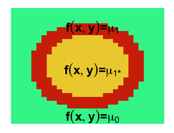
(a) Pattern $\mathcal{M}^{0}$

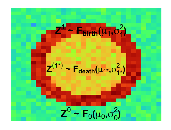
(b) Observed $\mathcal{M}^{\sigma}$

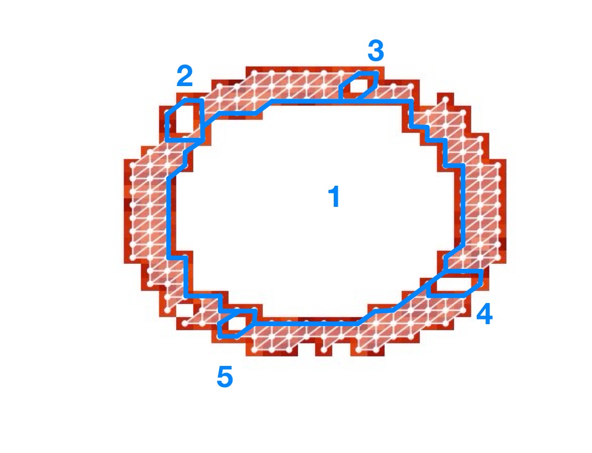
(c) $\delta$=3778 (birth)

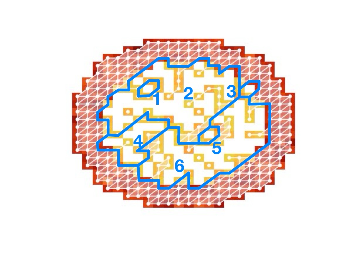
(d) $\delta$=3000

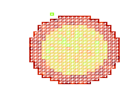
(e) $\delta$=2512 (death)

Figure 1: (a) Partitions of the underlying pattern into background $\mu_{0}$, loop $\mu_{1}$, and interior of the loop $\mu_{1*}$. (b) Partitions of the data into into background, the loop, and the interior of the loop. $Z^{k}$ where $k=\{0,1,1*\}$ represents a pixel intensity value and each $F_{k}$ is a distribution from which the pixel was drawn. (c) $\mathcal{K}_{3778}$ contains one connected component and five loops; 3778 is the birth time of the true loop (1). (d) $\mathcal{K}_{3000}$ contains five connected component and six loops. (e) $\mathcal{K}_{2512}$ contains two connected component and no loops, where 2512 is the death time of the large loop born at $\mathcal{K}_{3778}$.

The evolution of the homology groups of $\mathcal{M}$ over the course of the filtration is graphically represented on a persistence diagram $\mathcal{P}(\mathcal{M})$. Figure 2 shows an example of a persistence diagram of the data (Figure 1(b)) compared to the persistence diagram of the underlying pattern (Figure 1(a)) from which the data were generated. Features of each dimension, such as connected components and loops are represented in the diagram by displaying the death and birth times as (x,y) coordinates. Each homology group, is represented by a shape and color: connected components are black dots and loops are red triangles. The number of red triangles in each diagram is the number of loops detected in the upper-level set filtration for an image. The more persistent loops are farther from the diagonal line $y=x$.

In the persistence diagram for the data (Figure 2(a)), the birth time of the most persistent loop is $3778$ and the death time is $2512$, both of these are estimates of the birth and death time of the corresponding loop in the underlying pattern. All the other loops which are closer to the diagonal are small loops which are just due to noise. In the persistence diagram of the underlying pattern (Figure 2(b)) there is only one loop detected with a birth time of $4000$ and a death time of $3000$.

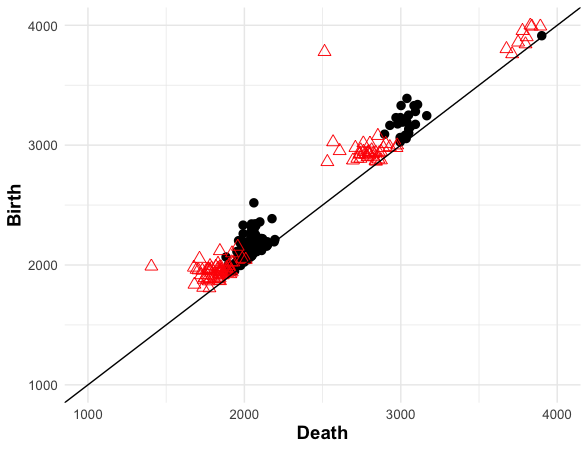
(a) Observed $\mathcal{P}(\mathcal{M}^{\sigma})$

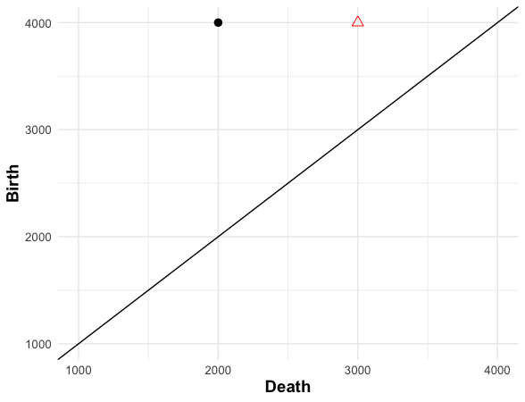
(b) Pattern $\mathcal{P}(\mathcal{M}^{0})$

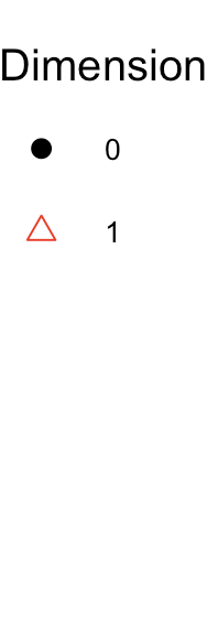
Figure 2: (a) The persistence diagram of the data in Figure 1(b) with loops (red triangles) and connected components (black dots). (b) The persistence diagram of the underlying pattern in Figure 1(a) which has only one loop and one connected component.

In the context of our application, a persistence diagram may be viewed as an estimate of the underlying pattern of $\mathcal{M}$, where a different realization of the image for the same data-generating process generally results in a different persistence diagram. The number of loops, and their corresponding birth and death times, can be an estimate of the pattern of the ring structure. In the next section, we outline a method to get uncertainty estimates for the birth and death times of the loops found in the data which allows for inference on the true persistence diagram Figure 2(b) from the observed persistence diagram Figure 2(a).

3 Confidence Regions for Persistence Diagram

In this section, we develop a method to assess the uncertainty in the estimated persistence diagram by constructing confidence regions around the birth and death times of the elements in $H_{1}(\mathcal{M^{\sigma}})$, the generators of the one-dimensional homology groups (i.e., loops). These confidence regions should cover the one-dimensional homology group generators of the persistence diagram of the noiseless true manifold $\mathcal{M}^{0}$. However, as is demonstrated in Section 4, there is considerable bias in the estimated birth and death times of loops using upper-level set filtrations for a raw image, which we refer to as the traditional TDA (tTDA) estimates.

An approach for reducing the influence of outliers when estimating persistence diagrams for point-cloud data uses upper-level set filtrations on kernel density estimates or regression models of the data, rather than a different type of filtration (e.g., a Vietoris-Rips filtration) on the point-cloud data directly (Chazal and Michel, 2021; Fasy et al., 2014). This technique is used in Fasy et al. (2014) to construct confidence regions on persistence diagrams for point-cloud data.

Since the confidence regions are centered around the estimated birth and death times, we need to obtain unbiased estimates of the birth and death times of loops in images. One possible approach, outlined in Section 3.5, is to estimate a smoother function of the image and doing an upper-level set filtration extending the inference approach in Fasy et al. (2014) from point-cloud data to a single image. We refer to this proposed extension as smooth TDA (sTDA). This is used as a comparison to our primary proposed approach which we refer to as partitioned TDA (parTDA). The parTDA method provides unbiased estimates without smoothing, and is presented in detail below in Section 3.2.

3.1 Setup

Let the image $\mathcal{M}$ be defined by some function $f(x,y)$ discretized onto a 2D grid $\mathcal{G}_{d_{1}\times d_{2}}$, where each (x,y) coordinate represents the grid columns $x=\{1,2,\ldots,d_{1}\}$ and grid rows $y=\{1,2,\ldots,d_{2}\}$. The true pattern is the noiseless image $\mathcal{M}^{0}=\{f(x,y):(x,y)\in\mathcal{G}\}$. However, in practice there is some zero-centered noise $\varepsilon(x,y)$ drawn from distribution $\mathbf{F}(0,\sigma^{2}(x,y))$ added to the function so that $\mathcal{M}^{\sigma}=\{f(x,y)+\varepsilon(x,y):(x,y)\in\mathcal{G}\}$ where the $\sigma$ exponent of $\mathcal{M}^{\sigma}$. Each grid value, or pixel, in $\mathcal{M}^{\sigma}$ has intensity $Z(x,y)$ drawn from:

$$Z(x,y)\sim\mathbf{F}(f(x,y),\sigma^{2}(x,y)),$$ (1)

where the mean is defined by $\mathcal{M}^{0}$ and the error is defined by $\varepsilon$.

In this work, the following assumptions are made regarding the topological features of the noise-free image, $\mathcal{M}^{0}$, which are estimated from the topological features of its noisy counterpart, $\mathcal{M}^{\sigma}$. The proposed method involves partitioning the image in a way that distinguishes the background and $n_{p}$ other topological structures (e.g., loops and the interior of loops).

Assumption 1.

The true image $\mathcal{M}^{0}$ can be segmented into contiguous regions with constant functional values: $f(x,y)=\mu_{k}$ $\forall$ $(x,y)$ within partition $\mathcal{G}_{k}$. Image $\mathcal{M}^{\sigma}$ can be segmented into $n_{p}+1$ contiguous regions where each region is defined as $\mathcal{M}^{\sigma}_{k}=\{f(x,y)+\varepsilon(x,y):(x,y)\in\mathcal{G}_{k}\}$ for $k=\{0,\ldots,n_{p}\}$ where $\mathcal{G}_{k}=\{(x,y)\in\mathcal{G}:f(x,y)=\mu_{k}\}$.

Assumption 2.

If the true image, $\mathcal{M}^{0}$, has at least one feature that is homeomorphic to a one-sphere (loop), let $n_{1}$ denote the number of one-spheres. Any partition of $\mathcal{M}^{0}$ that is homeomorphic to a one-sphere has pixel intensities fixed at $f(x,y)=\mu_{i}$ for $i=\{1,\ldots,n_{1}\}$ where $2n_{1}\leq n_{p}$, and the partition interior to this one-sphere has pixel intensities fixed at $f(x,y)=\mu_{i*}$. Let $\mu_{0}$ be designated as the mean of the background noise partition (if it exists).

Assumption 3.

For an upper-level set filtration assume for the majority of $i=\{1,\ldots,n_{1}\}$ that $\mu_{i}\geq\mu_{i*}$ and $\mu_{i}\geq\mu_{0}$.

If all the inequalities from Assumption Assumption 3 are $\geq$, for a given setting, then a an upper-level set filtration is sufficient. However, depending on how many $\mu_{i}\leq\mu_{i*}$, a lower-level set filtration may capture the topological features more effectively.

In Section 3.2, we develop the method to build confidence regions for an image with a single $H_{1}$ feature (i.e., loop) so that $n_{p}=3$ (background, $H_{1}$ feature, and the region interior to the $H_{1}$ feature). The method is generalized to multiple $H_{1}$ features in Section 3.3. Discussion on the partitioning of the images is presented in Section 3.4. Since we were unable to find a method of comparison in the literature, we propose an alternative method in Section 3.5 that extends the confidence region methodology of Fasy et al. (2014) from a point cloud to an image. This alternative method is used as a benchmark to compare to our segmentation method in Section 4.

3.2 Confidence regions for a single image with a single $H_{1}$ feature

Here we consider the setting with a single loop in $\mathcal{M}^{0}$. Assumptions Assumption 1 and Assumption 2 imply that $\mathcal{M}^{0}$ can be segmented into three contiguous regions where the background region is defined as $\mathcal{M}_{0}^{0}=\{\mu_{0}:(x,y)\in\mathcal{G}_{0}\}$, the part of the image homeomorphic to a one-sphere is defined as $\mathcal{M}_{1}^{0}=\{\mu_{1}:(x,y)\in\mathcal{G}_{1}\}$, and part of the image that is interior to this one-sphere is defined as $\mathcal{M}_{1*}^{0}=\{\mu_{1*}:(x,y)\in\mathcal{G}_{1*}\}$. For Sections 3.2 and 3.3, we assume the true partitions $\mathcal{G}_{0}$, $\mathcal{G}_{1}$, and $\mathcal{G}_{1*}$ are known. However, in practice the true partitions are unknown and segmentation is used to estimate each $\mathcal{G}_{k}$. Section 3.4 proposes an algorithm for reducing the bias in the confidence region coverage due to the misclassification of pixels in an estimated segmentation.

Using the known partitions, the data $\mathcal{M}^{\sigma}$ can be separated into three distributions from which pixels are drawn ($\mathcal{M}^{\sigma}_{0}$, $\mathcal{M}^{\sigma}_{1}$, $\mathcal{M}^{\sigma}_{1*}$) as defined in Assumptions Assumption 1:

$$\begin{split}\mathcal{M}^{\sigma}_{0}\text{ is the background partition where }Z^{0}\sim\mathbf{F_{0}}(\mu_{0},\sigma^{2}_{0})\\ \mathcal{M}^{\sigma}_{1}\text{ is the part homeomorphic to a one-sphere where }Z^{1}\sim\mathbf{F_{birth}}(\mu_{1},\sigma^{2}_{1})\\ \mathcal{M}^{\sigma}_{1*}\text{ is the part interior to the one-sphere where }Z^{1*}\sim\mathbf{F_{death}}(\mu_{1*},\sigma^{2}_{1*})\end{split}$$ (2)

The loop in the true pattern, of which we are trying to estimate its birth and death times, has a birth time of $\mu_{1}$ determined by $\mathcal{M}^{0}_{1}$ and a death time of $\mu_{1*}$ determined by $\mathcal{M}^{0}_{1*}$, as shown in Figure 1(a). In order to make the confidence regions, we define the joint distribution of the sample means of the pixel intensities associated with the birth and death times, $\bar{Z}^{1}$ and $\bar{Z}^{1*}$, respectively, as follows:

$$\mathbf{X}=\begin{pmatrix}\bar{Z}^{1*}\\ \bar{Z}^{1}\\ \end{pmatrix}\overset{\text{approx}}{\sim}\left(\begin{pmatrix}\mu_{1*}\\ \mu_{1}\end{pmatrix},\begin{pmatrix}\frac{\sigma_{1*}^{2}}{n_{d}}&0\\ 0&\frac{\sigma_{1}^{2}}{n_{b}}\end{pmatrix}\right)$$ (3)

where $n_{d}$ and $n_{b}$ are the number of pixels in $\mathcal{M}^{\sigma}_{1*}$ and $\mathcal{M}^{\sigma}_{1}$, respectively. By the Central Limit Theorem, $\mathbf{X}$ approximately follows a bivariate normal distribution allowing for a confidence region to be created based on: $\boldsymbol{(\bar{X}-\mu)^{T}\Sigma^{-1}(\bar{X}-\mu)}\sim\boldsymbol{\chi^{2}_{2}}$. The asymptotic confidence region for the birth and death times of $\mathcal{M}^{0}$ is as follows:

$$\boldsymbol{\mu}(\theta)=\boldsymbol{\bar{X}}+\sqrt{\boldsymbol{\chi^{2}_{2,\alpha}}}\sqrt{\boldsymbol{\hat{\Sigma}}}\begin{bmatrix}\text{cos}(\theta)\\ \text{sin}(\theta)\end{bmatrix}\text{ for }0<\theta<2\pi$$ (4)

where the variance can be estimated by sample variance.

The segmentation of $\mathcal{M}^{\sigma}_{k}$ for $k=\{0,1,1*\}$ creates the confidence regions in Equation (4) and the unbiased estimators for $(\mu_{1*},\mu_{1}):(\bar{Z}_{1*},\bar{Z}_{1})$. However, these unbiased estimates are not derived from an upper-level set filtration on $\mathcal{M}^{\sigma}$. This approach for generating confidence regions is called parTDA; next we describe the bias in tTDA methods.

3.2.1 Bias in traditional TDA birth and death times

The level of bias in the tTDA birth time is dependent on the proportion of the number of vertices of the simplicial complex that comprise the birth of the loop that are within the set of pixels associated with the corresponding true loop pattern. A similar bias is found with the tTDA death time and the relationship of the structure of the simplicial complex and the interior of the true pattern. A more technical explanation is provided next.

Assumption Assumption 3 states that $\mu_{1}\geq\mu_{0}$ and $\mu_{1}\geq\mu_{1*}$. When applying an upper-level set filtration to $\mathcal{M}^{\sigma}$, a number of loops can be identified along with the associated birth and death times $\{(d_{1},b_{1}),\dots,(d_{j},b_{j}),\ldots(d_{\beta_{1}},b_{\beta_{1}})\}$. Let $\beta_{1}$ be the total number of loops detected and $(d_{j},b_{j})$ be the tTDA birth and death times for the loop $\mathcal{M}^{\sigma}_{1}$ (topological signal). All other birth and death times are topological noise and not a part of the true pattern $\mathcal{M}^{0}$. The birth time, $b_{j}$, is the largest $\delta$ value in the filtration when the loop in $\mathcal{M}^{\sigma}_{1}$ first appears in the simplicial complex $\mathcal{K}_{b_{j}}=\{V_{b_{j}},K_{b_{j}}\}$. The part of the simplicial complex, $\mathcal{K}_{b_{j}}$, that comprises the birth of the loop is defined as follows:

$$\mathcal{K}_{\text{birth}}=\{V_{\text{birth}},K_{\text{birth}}\}\subseteq\mathcal{K}_{b_{j}}\text{ and }V_{\text{birth}}\subseteq\mathcal{G}_{1}.$$ (5)

Similarly, the death time, $d_{j}$, is the largest $\delta$ value in the filtration when the loop in $\mathcal{M}^{\sigma}_{1}$ disappears in the simplicial complex $\mathcal{K}_{d_{j}}=\{V_{d_{j}},K_{d_{j}}\}$. The part of the simplicial complex, $\mathcal{K}_{d_{j}}$, that makes up the interior of the loop is defined as follows:

$$\mathcal{K}_{\text{death}}=\{V_{\text{death}},K_{\text{death}}\}\subseteq\mathcal{K}_{d_{j}}\text{ and }V_{\text{death}}=\mathcal{G}_{1*}.$$ (6)

Figure 3 illustrates the difference between $b_{j},d_{j},\mathcal{K}_{b_{j}},\mathcal{K}_{\text{birth}},\mathcal{K}_{d_{j}},\mathcal{K}_{\text{death}},\mathcal{M}^{\sigma}_{1},\text{ and }\mathcal{M}^{\sigma}_{1*}$. The white rectangles in each subfigure outline $\mathcal{M}^{\sigma}_{1}$ (Figure 3(a)) or $\mathcal{M}^{\sigma}_{1*}$ (Figure 3(b)), the total purple simplicial complexes are either $\mathcal{K}_{b_{j}}$ (Figure 3(a)) or $\mathcal{K}_{d_{j}}$ (Figure 3(b)), while the part of the purple simplicial complexes within the white rectangles are either $\mathcal{K}_{\text{birth}}$ (Figure 3(a)) or $\mathcal{K}_{\text{death}}$ (Figure 3(b)). The black zero-simplex is the location of the pixel which has intensity $b_{j}$ (Figure 3(a)) or $d_{j}$ (Figure 3(b)). Note that any of the white rectangles beneath the purple simplicial complex appear light purple.

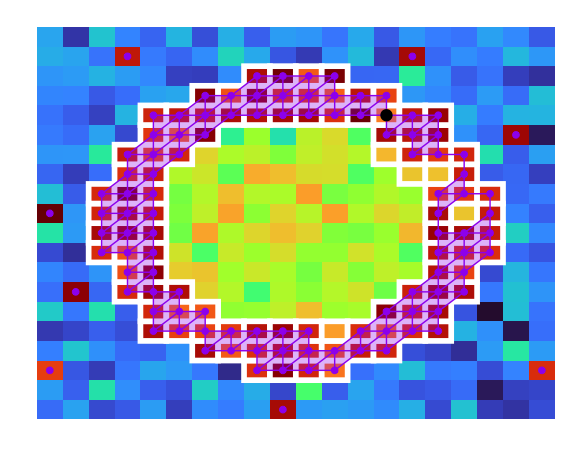
(a) $\mathcal{K}$ on $(\mathcal{M}^{\sigma})^{-1}(b_{j},\infty)$

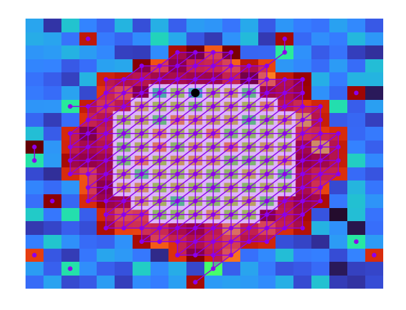
(b) $\mathcal{K}$ on $(\mathcal{M}^{\sigma})^{-1}(d_{j},\infty)$

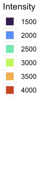
Figure 3: Illustration of simplicial complexes (purple) built on the upper-level sets at the birth time and death times of an image with a loop, with $\mu_{1}=4000$ and $\mu_{1*}=3000$. (a) The simplicial complex $\mathcal{K}_{b_{j}}=\mathcal{K}_{3597}$ at the birth of the loop where the black dot is the pixel with intensity value equal to 3597, which is the upper-level set threshold associated with the birth of the loop. The white rectangles indicate the pixels of $\mathcal{M}^{\sigma}_{1}$. (b) The simplicial complex $\mathcal{K}_{d_{j}}=\mathcal{K}_{2593}$ at the death of the loop where the black dot is the pixel with intensity value equal to 2593, which is the upper-level set threshold associated with the death of the loop. The white rectangles, which indicate the pixels of $\mathcal{M}^{\sigma}_{1*}$, appear light purple due to the overlaying two-simplices in $\mathcal{K}_{d_{j}}$.

The level of bias in the estimate of $b_{j}$ using tTDA depends on the proportion between the number of elements in the set $\mathcal{K}_{\text{birth}}$ and the number of elements in the set $\mathcal{G}_{1}$, represented by $p_{b}$. According to Equation 5, where $Z(V_{\text{birth}})\subseteq\mathcal{M}^{\sigma}_{1}$ and $Z^{1}\sim F_{\textbf{birth}}(\mu_{1},\sigma^{2}_{1})$, the proportion $p_{b}$ is defined as follows:

$$p_{b}=1-\dfrac{|V_{\text{birth}}|}{|\mathcal{M}^{\sigma}_{1}|}=1-\dfrac{|V_{\text{birth}}|}{n_{b}},$$ (7)

where $|X|$ is the cardinality of the set $X$.

Since the birth time is the minimum intensity values of all the pixels $Z^{1}(x,y)$ where $(x,y)\in V_{\text{birth}}$, then $F_{\textbf{birth}}^{-1}(p_{b})=b_{j}$. The bias in the birth time is:

$$\text{Bias}(\mu_{1},b_{j})=\mu_{1}-E\{F_{\textbf{birth}}^{-1}(p_{b})\}.$$ (8)

The birth time is unbiased if $b_{j}$ falls within the $50^{\text{th}}$ percentile of all pixels comprising loop $Z^{1}$, given that $F_{\textbf{birth}}$ is a symmetric distribution.

The level of bias of $d_{j}$ (using tTDA) depends on the proportion between the number of elements in the set $\mathcal{K}_{\text{death}}$ and the number of elements in the set $\mathcal{G}_{1*}$, denoted by $p_{d}$. Based on the Assumptions in Section 3, all the pixels which make up the interior of the loop are a part of the simplicial complex at the death of the loop. From Equation 6, $Z(V_{\text{death}})\subseteq\mathcal{M}^{\sigma}_{1*}$ and $Z^{1*}\sim F_{\textbf{death}}(\mu_{1*},\sigma^{2}_{1*})$ and consequently, the proportion $p_{d}$ is:

$$p_{d}=1-\dfrac{|V_{\text{death}}|}{|\mathcal{M}^{\sigma}_{1*}|}=1-\dfrac{n_{d}}{n_{d}}=0.$$ (9)

Then $F_{\textbf{death}}^{-1}(0)=\min(Z^{1*})=d_{j}$ where the bias in the estimate is:

$$\text{Bias}(\mu_{1*},d_{j})=\mu_{1*}-E\{\min(Z^{1*})\}.$$ (10)

Therefore, the death time is an unbiased estimator of $\mu_{1*}$ when there is only one pixel which makes up $\mathcal{M}^{\sigma}_{1*}$ since $E(\text{min}(Z^{1*}))=E(Z^{1*})=\mu_{1*}$.

Figure 4 displays results of an exploration of the relationship between bias in tTDA estimates of the birth and death times and the construction of the image, compared to the unbiased parTDA estimates. Differences in the image dimension and the area of the partitions ($\mathcal{G}^{\sigma}_{1}$ and $\mathcal{G}^{\sigma}_{1*}$) change the amount of bias in the tTDA estimates of the birth and death times of the loop. Two simulations studies are carried out: (1) considers four different loop thickness levels and (2) considers four different different image dimensions levels;. Each factor level for both simulations has 100 iid images generated with one loop ($(\mu_{1*},\mu_{1})=(3000,4000)$). At each of the loop thickness level, $\{1,2,3,4\}$, the birth and death times of the loop $(d_{j},b_{j})$ is calculated for each image. Level 1 is for a very thin loop (two pixels thick), level 2 is a medium thin loop (seven pixels thick), level 3 is a medium thick loop (11 pixels thick), and level 4 is for a thick loop (16 pixels thick). Similarly, at each image dimension level, $\{20\times 20,50\times 50,100\times 100,150\times 150\}$, the birth and death times of the loop $(d_{j},b_{j})$ are calculated for each image. These results are shown in boxplots in Figure 4, where the light blue boxplots are the tTDA birth and death times while the red boxplots are the parTDA birth and death times.

As seen in Figure 4, estimates of the birth (Figure 4(a)) and death (Figure 4(b)) times across all different factor levels (dimension and thickness) using parTDA are unbiased. Whereas, estimates of the birth and death times using tTDA are biased and this bias changes depending on different factor levels.

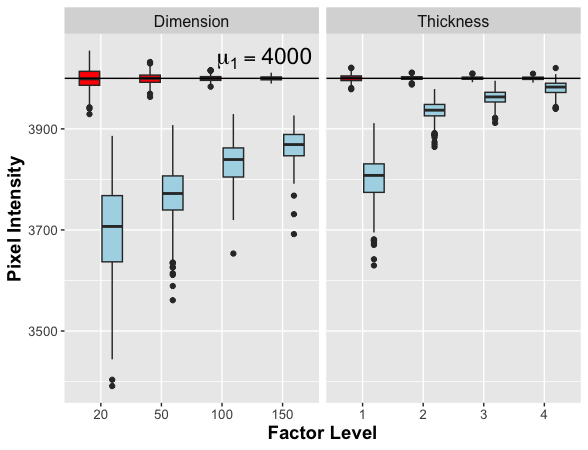
(a) Birth times $(b_{j})$

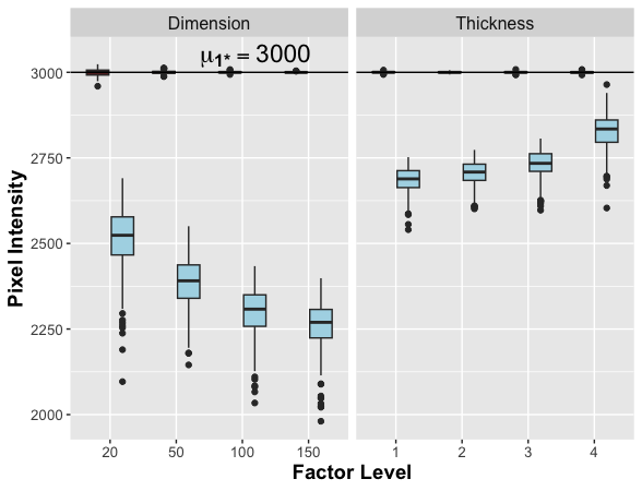
(b) Death Times $(d_{j})$

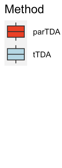
Figure 4: Boxplots illustrating estimated birth (a) and death (b) times of loops using parTDA (red) and tTDA (blue), based on 100 iid images within each factor Level of loop thickness or dimensions. The true birth and death times are indicated by the horizontal solid black lines. The tTDA estimates have a strong negative bias with higher variability, while the proposed parTDA estimates appear to be unbiased with lower variability.

When interpreting Figure 4, the dimension of the image serves as a proxy for the pixel sample size of the partitions, with higher dimensions indicating larger sample sizes in both $\mathcal{M}^{\sigma}_{1}$ and $\mathcal{M}^{\sigma}_{1*}$. As image dimension increases, the bias in the birth time estimates using tTDA decreases as well as the variance. However, for the death time, the bias increases as the image dimensions increase. This results is consistent with the discussion of $p_{d}$ in Equation 9. Loop thickness, which is really looking at area of $\mathcal{M}^{\sigma}_{1}$ and $\mathcal{M}^{\sigma}_{1*}$, has less bias in both the birth and death times. In general, thicker loops or larger image dimensions (more pixels making up the loop) lead to less biased estimates of the birth time. Thicker loops or smaller image dimensions (fewer pixels making up the inside of the loop) lead to less biased estimates of the death time. In certain situations the tTDA estimate, $(d_{j},b_{j})$ is an unbiased estimator for $(\mu_{1*},\mu_{1})$ whereas, $(\bar{Z}_{1*},\bar{Z}_{1})$ is unbiased regardless of the way the loop or image is constructed.

3.2.2 Matching loops between tTDA and parTDA

The partitions $\mathcal{G}_{k}$ used in parTDA to estimate the birth and death times of a loop do not directly use TDA (e.g., there is no assumption that a partition forms a loop). To detect a loop, the unbiased estimates, $(\bar{Z}^{1*},\bar{Z}^{1})$, need to be matched to a corresponding loop detected from tTDA, $(d_{j},b_{j})$, for a loop to be detected with parTDA. Algorithm 1 is designed to identify which of the loops in the $\mathcal{M}^{\sigma}$, $\{(d_{1},b_{1}),\ldots,(d_{j},b_{j}),\ldots(d_{\beta_{1}},b_{\beta_{1}})\}$, are in the partitions $\mathcal{G}_{1*}$ and $\mathcal{G}_{1}$ by the location of the birth and death time pixel intensities. The loops which are not matched to the partitions are not considered to be part of the underlying pattern. Once $(d_{j},b_{j})$ is matched with the partitions $(\mathcal{G}_{1*},\mathcal{G}_{1})$ using Algorithm 1, then the birth and death times of the loop detected with tTDA are then estimated with $(\bar{Z}_{1*},\bar{Z}_{1})$.

1:Input: $df\coloneqq(x,y,Z[x,y])$ of image $\mathcal{M}^{\sigma}$; partitions $\mathcal{G}_{k}$ for $k=\{0,1,1*\}$, birth and death times from $\mathcal{P}(M^{\sigma})\coloneqq\{(d_{1},b_{1}),\ldots,(d_{m},b_{m})\}$.

2:Output: $(d_{j},b_{j})$ matched to $(\mathcal{G}_{1*},\mathcal{G}_{1})$

3:Define: $df_{k}=\{(x,y,Z[x,y])\in\mathcal{G}_{k}\}$, $k=\{0,1,1*\}$; out${}_{d}=\emptyset$; out${}_{b}=\emptyset$; out$=\emptyset$

4:for l in 1:m do

5:     Step 1: Find $df_{k}$ where $Z(x,y)=d_{l}$ $\triangleright$ Identify pixel location of $d_{l}$ in $\mathcal{G}$

6:     if $k=1*$ then out${}_{d}\leftarrow$ out${}_{d}\cup l$ $\triangleright$ Only keep index $l$ for $d_{l}\in\mathcal{G}_{1*}$

7:     end if

8:     Step 2: Find $df_{k}$ where $Z(x,y)=b_{l}$ $\triangleright$ Identify pixel location of $b_{l}$ in $\mathcal{G}$

9:     if $k=1$ then out${}_{b}\leftarrow$ out${}_{b}\cup l$ $\triangleright$ Only keep index $l$ for $b_{l}\in\mathcal{G}_{1}$

10:     end if

11:     Step 3: Calculate out$\leftarrow$out${}_{d}\cap$ out_b

12:     if length($out$)==2 then $(d_{l},b_{l})=(d_{j},b_{j})$ $\triangleright$ If $b_{l}\in\mathcal{G}_{1}$ and $d_{l}\in\mathcal{G}_{1*}$ loop is matched

13:         Stop $\triangleright$ Match found, stop algorithm

14:     end if

15:end for

16:return out

Algorithm 1 Localizing the birth and death times $(d_{j},b_{j})$

3.3 Confidence regions for multiple $H_{1}$ features

Section 3.2 introduces parTDA for the setting with only one loop in $\mathcal{M}^{0}$, which is the setting of our motivating cell image application presented in Section 5. The objective of this section is to explain how the proposed method can be generalized to encompass multiple loops within a single image. While the primary emphasis is on one-spheres, it is worth noting that the methodology can be readily extended to $p$-spheres for higher-dimensional spaces, such as 3D images.

Assume that there are $n_{1}$ loops in $\mathcal{M}^{0}$ resulting in $2n_{1}+1$ partitions and that the functional value of each loop in $f(x,y)$ is $\mu_{i}$ and the value of the interior of each one-sphere in $f(x,y)$ is $\mu_{i*}$ for $i=\{1,\ldots n_{1}\}$. For every loop of $\mathcal{M}^{0}$, the persistence diagram of the observed image represents each loop as birth death pairs: $(d_{j_{1}},b_{j_{1}}),\ldots(d_{j_{n_{1}}},b_{j_{n_{1}}})$. The steps listed in Algorithm 1 can be extended to connect each $(d_{j_{i}},b_{j_{i}})$ with $(\mathcal{G}_{i*},\mathcal{G}_{i})$ where the partitions $\mathcal{G}_{k}$ become $k=\{0,i,i*\}$ for $i=\{1,\ldots,n_{1}\}$.

There are three other possible types of birth-death pairs $(d_{l},b_{l})$ where $l\neq j_{i}$ for $i=\{1,\ldots n_{1}\}$ detected in the image $\mathcal{M}^{\sigma}$ which are not loops in $\mathcal{M}^{0}$:

(1) loops which are in the background ($d_{0},b_{0}\sim\mathbf{F}_{0}(\mu_{0},\sigma_{0}^{2})$)

$$d_{0}\notin\mathcal{M}^{\sigma}_{i*}\text{ and }b_{0}\notin\mathcal{M}^{\sigma}_{i}\forall i\neq 0\implies\text{using Algorithm \ref{alg:Seg1H1} }(d_{0},b_{0})\neq(d_{j_{i}},b_{j_{i}})$$ (11)

(2) loops which are only in $\mathcal{M}_{i}$ or only in $\mathcal{M}_{i*}$ ($d_{i},b_{i}\sim\mathbf{F}_{\textbf{birth}}(\mu_{i},\sigma_{i}^{2})$ or $d_{i*},b_{i*}\sim\mathbf{F}_{\textbf{death}}(\mu_{i*},\sigma_{i*}^{2})$)

$$d_{i},b_{i}\in\mathcal{M}^{\sigma}_{i} \implies\text{using Algorithm~{}\ref{alg:Seg1H1} }(d_{i},b_{i})\neq(d_{j_{i}},b_{j_{i}})$$ (12)

$$d_{i*},b_{i*}\in\mathcal{M}^{\sigma}_{i*} \implies\text{using Algorithm~{}\ref{alg:Seg1H1} }(d_{i*},b_{i*})\neq(d_{j_{i}},b_{j_{i}})$$ (13)

(3) loops that traverse the background and $\mathcal{M}_{i}^{\sigma}$ ($b_{i}\sim\mathbf{F}_{\textbf{birth}}(\mu_{i},\sigma^{2}_{i})$ and $d_{0}\sim\mathbf{F}_{0}(\mu_{0},\sigma^{2}_{0})$)

$$d_{0}\notin\mathcal{M}^{\sigma}_{i*}\implies\text{using Algorithm~{}\ref{alg:Seg1H1} }(d_{0},b_{i})\neq(d_{j_{i}},b_{j_{i}})$$ (14)

Since all the loops detected in the segmentation $\mathcal{M}^{\sigma}_{i}$ are connected to the correct $(d_{j_{i}},b_{j_{i}})$, the only time a problem would arise is when $d_{j_{i}}=d_{j_{k}}$ and $b_{j_{i}}=b_{j_{k}}$ for $i\neq k$ where $i,k\in\{1,\ldots,n_{1}\}$. In other words, if the loop $\mathcal{M}^{\sigma}_{i}$ and the loop in $\mathcal{M}^{\sigma}_{k}$ have the exact same birth and death times, the algorithm would not be able to match $(d_{j_{i}},b_{j_{i}})$ and $(d_{j_{k}},b_{j_{k}})$ with $(\mathcal{G}_{i*},\mathcal{G}_{i})$ and $(\mathcal{G}_{k*},\mathcal{G}_{k})$, respectively. However, this situation would happen with zero probability since all $Z^{i}\sim\mathbf{F}_{\textbf{birth}}(\mu_{i},\sigma_{i}^{2})$, $Z^{k}\sim\mathbf{F}_{\textbf{birth}}(\mu_{k},\sigma_{k}^{2})$ and $Z^{i*}\sim\mathbf{F}_{\textbf{death}}(\mu_{i*},\sigma_{i*}^{2})$, $Z^{k*}\sim\mathbf{F}_{\textbf{death}}(\mu_{k*},\sigma_{k*}^{2})$ are continuous distributions.

3.4 Segmentation of the image

In the preceding two subsections the partitions $\mathcal{G}_{k}$ for $k=\{0,\ldots,n_{p}\}$ are assumed to be known; whereas in this section, the segmentation is unknown and is estimated with $\mathcal{\hat{G}}_{k}$ for $k=\{0,\ldots,\hat{n}_{p}\}$. If the segmentation is incorrect the parTDA estimated birth and death times in Equation (3) and the corresponding confidence regions in Equation (4) may not be accurate. Here, we propose a method to reduce the misclassification of pixels in partitions when one or more of the $\mathcal{\hat{G}}_{k}$’s may have some incorrect pixels assigned to it.

Recall from Equation 2 that if $\mathcal{G}_{k}$ is known $\forall k\in\{0,\ldots,n_{p}\}$ then interior pixel intensities $Z^{i*}\sim F_{\textbf{death}}(\mu_{i*},\sigma_{i*}^{2})$ for every $Z^{i*}\in\mathcal{M}^{\sigma}_{i*}$ and pattern pixel intensities $Z^{i}\sim F_{\textbf{birth}}(\mu_{i},\sigma_{i}^{2})$ for every $Z^{i}\in\mathcal{M}^{\sigma}_{i}$, where $i\in\{1,\ldots,n_{1}\}$, with the number of pixels in the sets defined as $|\mathcal{M}^{\sigma}_{i}|=n_{b}^{i}$, and $|\mathcal{M}^{\sigma}_{i*}|=n_{d}^{i}$.

When $\mathcal{G}_{k}$, is unknown $\mathcal{\hat{M}}^{\sigma}_{i}$ and $\mathcal{\hat{M}}^{\sigma}_{i*}$ are estimated using some segmentation procedure. Any segmentation procedure may be used to estimate the partitions, as long as the resulting partitions are contiguous regions. In this paper, we apply edge detection methods to segment the image by identifying edges, which are located at the maxima of the gradient strength obtained from a Laplacian of the Gaussian-smoothed image (Canny, 1986; Parker, 2010). For certain parameter values, the edge contours are closed creating contiguous regions and the standard deviation of the filter changes how many regions are detected. Let $\hat{e}$ be the edge set which segments the image $\mathcal{M}^{\sigma}$ into partitions $\mathcal{\hat{G}}_{k}$.

Assume that some part of the segmentation of a loop or its interior is incorrect so that $\mathcal{\hat{G}}_{k}\neq\mathcal{G}_{k}$ for $k=\{i,i*\}$ for some $i$. Then there are $m_{d}$ pixel intensities, denoted by $\tilde{Z}^{i*}$, in the set $\mathcal{M}_{i*}$ which are misclassified into $\mathcal{\hat{M}}_{i}$ (i.e., these are the pixels that should be a part of the interior, but were assigned to the loop). Similarly, there are $m_{b}$ pixel intensities, denoted by $\tilde{Z}^{i}$, in the set $\mathcal{M}_{i}$ which are misclassified into $\mathcal{\hat{M}}_{i*}$ (i.e., these are the pixels that should be a part of the loop, but were assigned to the interior). There are then $n_{d}-m_{d}$ pixel intensities, denoted by $\tilde{\tilde{Z}}^{i*}$, in the set $\mathcal{M}_{i*}$ which are correctly classified into $\mathcal{\hat{M}}_{i*}$ and there are $n_{b}-m_{b}$ pixel intensities, denoted by $\tilde{\tilde{Z}}^{i}$, in the set $\mathcal{M}_{i}$ which are correctly classified into $\mathcal{\hat{M}}_{i}$.

The set of pixels which comprise the interior of the loop $Z^{i*}$ and the set of pixels which comprise the loop $Z^{i}$ can be decomposed as follows:

$$Z^{i*}=\tilde{\tilde{Z}}^{i*}\cup\tilde{Z}^{i*}\text{ and }Z^{i}=\tilde{\tilde{Z}}^{i}\cup\tilde{Z}^{i}.$$ (15)

$\mathcal{\hat{M}}_{i*}$ denotes all the pixels which are classified as interior pixels of the loop $\mathcal{\hat{G}}_{i*}$ (i.e., $\mathcal{\hat{M}}_{i*}=\tilde{\tilde{Z}}^{i*}\cup\tilde{Z}^{i}$) and $\mathcal{\hat{M}}_{i}$ denotes all the pixels which are classified as loop pixels $\mathcal{\hat{G}}_{i*}$ (i.e., $\mathcal{\hat{M}}_{i}=\tilde{\tilde{Z}}^{i}\cup\tilde{Z}^{i*}$). Therefore $n_{b}-m_{b}+m_{d}$ pixels are in the birth time partition $\mathcal{\hat{G}}^{\sigma}_{i}$ and $n_{d}-m_{d}+m_{b}$ pixels are in the death time partition $\mathcal{\hat{G}}^{\sigma}_{i*}$.

The expected value of the (biased) estimators of the birth and death time using the incorrect partitions of the loop are:

$$E(\bar{\mathcal{\hat{M}}}_{i})=\frac{(n_{b}-m_{b})\mu_{i}+m_{d}\mu_{i*}}{n_{b}-m_{b}+m_{d}}\text{ and }E(\bar{\mathcal{\hat{M}}}_{i*})=\frac{(n_{d}-m_{d})\mu_{i*}+m_{b}\mu_{i}}{n_{d}-m_{d}+m_{b}},$$ (16)

where $\bar{\mathcal{\hat{M}}}_{i}$ and $\bar{\mathcal{\hat{M}}}_{i*}$ are the sample means of the sets of pixels $\mathcal{\hat{M}}_{i}$ and $\mathcal{\hat{M}}_{i*}$, respectively.

By Assumption Assumption 3, $\mu_{i*}\leq\mu_{i}$ and assuming that the segmentation $\mathcal{\hat{G}}_{i}$ and $\mathcal{\hat{G}}_{i*}$ are close to the true $\mathcal{G}_{i}$ and $\mathcal{G}_{i*}$ (i.e., only a few pixels are misclassified), then $m_{b}<n_{d}$ and $m_{d}<n_{b}$ and any $\tilde{Z}^{i}\in\mathcal{\hat{M}}_{i*}$ and $\tilde{Z}^{i*}\in\mathcal{\hat{M}}_{i}$ are neighbors of the edge set $\hat{e}$ (i.e., $\tilde{Z}^{i},\tilde{Z}^{i*}\in n_{c}(\hat{e})$ where $c$ is the unit distance between two pixels.

Let $q^{i}_{1},q^{i*}_{1}$ be the first quantiles and $q^{i}_{3},q^{i*}_{3}$ be the third quantiles of $F_{\textbf{birth}}$, $F_{\textbf{death}},$ respectively. Assume that the noise distribution $\varepsilon(x,y)\sim\mathbf{F}(0,\sigma^{2}(x,y))$ is symmetric. An assumption of Algorithm 2 is that the distribution of the interior pixel intensities and the pattern pixel intensities are well-separated, as described in the following.

Assumption 4.

Assume that $(o_{i}-T(\tilde{\mu}_{i}))<(o_{i}-\tilde{T}(\mu_{i*}))$ and $(o_{i*}-T(\tilde{\mu}_{i*}))<(o_{i*}-T(\tilde{\mu}_{i}))$ where $o_{i}$ is an outlier in the distribution $F_{\textbf{birth}}$ and $o_{i*}$ is an outlier in the distribution $F_{\textbf{death}}$. $T(\tilde{\mu}_{i*})$ and $T(\tilde{\mu}_{i})$ are the truncated means of $F_{\textbf{birth}},F_{\textbf{death}}$ with upper bound $q^{i*}_{3}+1.5(q^{i*}_{3}-q^{i*}_{1})$ and lower bound $q^{i}_{3}+1.5(q^{i}_{3}-q^{i}_{1})$, respectively.

Under these assumption, Algorithm 2 sorts the $m_{b}$ and $m_{d}$ misclassified pixels, $\tilde{Z}^{i}$ and $\tilde{Z}^{i*}$, into the edge set $\hat{e}$ and keep the outliers, $\tilde{\tilde{Z}}^{i}\sim\mathcal{M}^{\sigma}_{i}$ and $\tilde{\tilde{Z}}^{i*}\sim\mathcal{M}^{\sigma}_{i*}$ in the correct segments $\mathcal{\hat{M}}^{\sigma}_{i}$, $\mathcal{\hat{M}}^{\sigma}_{i*}$.

As an illustration of the performance of Algorithm 2, the following experiment was carried out and results are displayed in Figure 5. For three different noise settings $(\sigma=\{50,100,300\})$, 100 iid images with one loop, similar to Figure 1(b) with $(\mu_{1*},\mu_{1})=(1000,3000)$, are generated and segmented incorrectly with the same edge set $\hat{e}$. In this example, six pixels are misclassified in the loop (i.e., $\tilde{Z}^{1*}\in\mathcal{\hat{G}}_{1}$) with the edge set $\hat{e}$. The 95% confidence regions using parTDA are calculated using both this misclassified partition $\hat{e}$ and the corrected partion $\hat{e}_{\text{new}}$ generated from Algorithm 2. Lower noise levels have more biased coverage of the resulting confidence regions compared to the higher noise levels.

Input: edge set $\hat{e}$; image $\mathcal{M}^{\sigma}$; partitions $\mathcal{\hat{G}}_{1}$ and $\mathcal{\hat{G}}_{1*}$; $c$=pixel side length

Output: new edge set $\hat{e}^{\text{new}}$

Define: $\mathcal{\hat{M}}^{\sigma}_{i}=\{Z^{i}(x,y)_{l}:(x,y)_{l}\in\mathcal{\hat{G}}_{i}\}$, $L_{i}=|\mathcal{\hat{M}}^{\sigma}_{i}|,$ $P(Z^{i}(x,y)\leq q^{i}_{1})=0.25$, $P(Z^{i}(x,y)\leq q^{i}_{3})=0.75$ for $i=\{1,1*\}$; outlier${}_{i}=\emptyset$; outlier.idx${}_{i}=\emptyset$; dist()=Euclidean distance; $e_{1}=\emptyset$

for i in $\{1,1*\}$ do

     for l in $1:L_{i}$ do $\triangleright$ Check if $Z^{i}(x,y)_{l}$ is an outlier and neighbors an edge in $\mathcal{\hat{G}}_{i}$

         if $\left((Z^{i}(x,y)_{l}>q^{i}_{3}+1.5(q^{i}_{3}-q^{i}_{1}))\mid(Z^{i}(x,y)_{l}<q^{i}_{1}-1.5(q^{i}_{3}-q^{i}_{1}))\right)$ &

$\left(\exists(\tilde{x},\tilde{y})\in\hat{e}~{}s.t.~{}\text{dist}((x,y)_{l},(\tilde{x},\tilde{y}))\leq\sqrt{2}c\right)$ then$\text{ outlier}_{i}\leftarrow\text{outlier}_{i}\cup Z^{i}(x,y)_{l}$, outlier.idx${}_{i}\leftarrow\text{outlier.idx}_{i}\cup l$

         end if

     end for

end for

Calculate $\hat{\mu}_{1}=\mathcal{\hat{M}}^{\sigma}_{1}\setminus$outlier₁ and $\hat{\mu}_{1*}=\mathcal{\hat{M}}^{\sigma}_{1*}\setminus$outlier_1∗ $\triangleright$ Calculate means without outliers

for i in $\{1,1*\}$ do

     for l in outlier.px_i do

         if $|Z^{i}(x,y)_{l}-\hat{\mu}_{i}|\geq|Z^{i}(x,y)_{l}-\hat{\mu}_{i^{c}}|$ then $\triangleright$ $i^{c}$ is the complement in $\{1,1*\}$ for $i$ $e_{1}\leftarrow e_{1}\cup(x,y)_{l}$ $\triangleright$ only add $(x,y)_{l}$ to new edge set $e_{1}$ if $Z^{i}(x,y)_{l}$ is closer to $\hat{\mu}_{i^{c}}$

         end if

     end for

end for

$\hat{e}^{\text{new}}=\hat{e}\cup e_{1}$

return $\hat{e}^{\text{new}}$

Algorithm 2 Remove Misclassified Pixels from Partition ($\mathcal{G}_{1}$,$\mathcal{G}_{1*}$)

Figure 5(a) shows all 100 estimated 95% confidence regions built using $\hat{e}$ (red) and $\hat{e}_{\text{new}}$ (blue) for the different $\sigma$ values. The green dot is the true $(\mu_{1*},\mu_{1})=(1000,3000)$ which the regions should cover $95\%$ of the time, on average. The confidence regions for the misclassified setting are underestimating $\mu_{1}$ since some $Z^{1*}s$ pixel intensities, which are lower than those of $Z^{1}$, are included in the $\bar{Z}^{1}$ resulting in an estimate that is biased low. After Algorithm 2 is applied, the bias in the confidence regions appear to be corrected in terms of the birth time.

In Figure 5(b), the coverage is calculated based on 100 iid images at each noise level $(\sigma=\{10,50,100,200,300\})$. The misclassified boxplots (red) show the coverage of the confidence regions built from $\hat{e}$, and the corrected boxplots (blue) show the coverage for confidence regions calculated with the $\hat{e}^{new}$ after running Algorithm 2. As illustrated in both plots, the algorithm significantly improves the coverage of the confidence regions. Correct segmentation is crucial for parTDA, and this section emphasizes the importance of checking the segmentation.

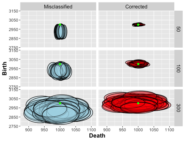
(a) Example of confidence regions

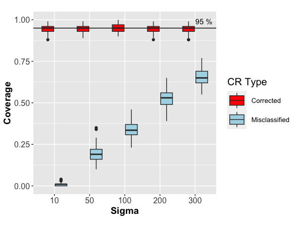
(b) Coverage of confidence regions

Figure 5: Confidence regions and coverage before (misclassified) and after (corrected) Algorithm 2 has been applied. The misclassified segmentation $\hat{e}$ has six pixels incorrectly classified. (a) Confidence regions for 100 images at noise level $\sigma=\{50,100,300\}$ are shown using $\hat{e}$ (misclassified) and $\hat{e}_{\text{new}}$ (corrected). The green dots indicate the true birth and death time location. (b) The coverage of the 95% confidence regions for $\sigma=\{10,50,100,200,300\}$ for misclassified (red) and corrected (blue) segmentations, using 100 iid images.

3.5 Alternative Method

We extend one of the methods from Fasy et al. (2014) from point-cloud data to handle an image as a way to establish a benchmark, because we are unaware of a direct basis for comparison with parTDA. In this approach, a distance metric is used to derive the distribution of distances between the persistence diagrams of the smoothed data, $\mathcal{P}(\mathcal{\tilde{M}}^{\sigma})$, and the persistence diagram of the true pattern, $\mathcal{P}(\mathcal{\tilde{M}}^{0})$.

Persistence diagram stability results (Cohen-Steiner et al., 2005) are used to bound the (bottleneck) distance between the persistence diagrams by the $L_{\infty}$ distance between kernel density estimates (KDEs) of the point-cloud data and the true pattern. Asymptotic confidence regions are then built from the distribution of $L_{\infty}$ distances between $\mathcal{\tilde{M}}^{\sigma}$ and $\mathcal{\tilde{M}}^{0}$, which can be estimated using a bootstrap procedure.

This procedure is briefly outlined below and then followed by the proposed adjustments for image data. See Section 3.4 of Fasy et al. (2014) for more details.

In the context of Fasy et al. (2014), let $\mathcal{M}^{\sigma}$ be point-cloud data. One of their proposed methods for persistence diagram confidence regions considers a KDE of $\mathcal{M}^{\sigma}$, $\mathcal{\tilde{M}}^{\sigma}$, to estimate the true birth and death time, $(\tilde{\mu}_{i*},\tilde{\mu}_{i})$, of the (true) smoothed manifold, $\mathcal{\tilde{M}}^{0}$. They define an asymptotic $(1-\alpha)100$% confidence regions, adapted to our notation which omits the dependency on bandwidth and sample size; see Theorem 12 of Fasy et al. (2014) for the precise statements:

$$\mathbb{P}\left(\mathcal{W}_{\infty}(\mathcal{P}(\mathcal{\tilde{M}}^{\sigma}),\mathcal{P}(\mathcal{\tilde{M}}^{0}))>c_{n}\right)\leq\mathbb{P}\left(||\mathcal{\tilde{M}}^{\sigma}-\mathcal{\tilde{M}}^{0}||_{\infty}>c_{n}\right)\leq\alpha+O\left(n^{-1/2}\right)$$ (17)

where $c_{n}$ defines the confidence region based on the data, and the first inequality follows from the stability result of Cohen-Steiner et al. (2005). The bottleneck distance, $\mathcal{W}_{\infty}$ is defined as

$$W_{\infty}(\mathcal{P}(\mathcal{\tilde{M}}^{\sigma}),\mathcal{P}(\mathcal{\tilde{M}}^{0}))=\inf_{\eta:\mathcal{P}(\mathcal{\tilde{M}}^{\sigma})\longrightarrow\mathcal{P}(\mathcal{\tilde{M}}^{0})}\sup_{(b,d)\in\mathcal{P}(\mathcal{\tilde{M}})}||(b,d)-\eta(b,d)||_{\infty}$$ (18)

where $\eta$ is a bijection of the features of the diagrams, including the diagonal $b=d$ line (Cohen-Steiner et al., 2005; Fasy et al., 2014). Since $\mathcal{\tilde{M}}^{0}$ is unknown and there is only one realization of the data $\mathcal{\tilde{M}}^{\sigma}$, a bootstrap approach is used. In particular, the estimate of $c_{n}$ is the $(1-\alpha)$-quantile of the distribution of the $L_{\infty}$ distances between the smoothed data $\mathcal{\tilde{M}}^{\sigma}$ and smoothed bootstrap realizations of the point-cloud data.

To implement this alternative approach two modifications are made: (1) Instead of a KDE on point clouds, we use local polynomial smoothing to change the raw image $\mathcal{M}^{\sigma}$ into a smoothed image $\mathcal{\tilde{M}}^{\sigma}$. In Section 4, we use degree two polynomials and an adaptive bandwidth of 0.3 as parameter inputs for local polynomial smoothing. These input values resulted in only one loop detected by an upper-level set filtration for the smoothed pattern, $\mathcal{\tilde{M}}^{0}$, analogous to the original image, $\mathcal{M}^{0}$. This facilitates the comparison between sTDA and parTDA. Note that sTDA builds confidence regions to cover $(\tilde{\mu}_{i*},\tilde{\mu}_{i})$ (i.e., death and birth times of loops in $\mathcal{\tilde{M}}^{0}$) whereas parTDA builds confidence regions to cover $(\mu_{i*},\mu_{i})$ (i.e., death and birth times of loops in $\mathcal{M}^{0}$). (2) We propose a method to bootstrap an image as opposed to a point cloud. The traditional bootstrap method assumes that each observation is iid which is not a suitable assumption for an image which typically have spatial correlation. Similar to parTDA, we segment the image into different strata and use the stratified bootstrap to resample the full image. Within each stratum the pixels can be viewed as being drawn from the same distribution, so pixel intensities within each stratum can be bootstrapped. In our simulation study, the number of strata and the segmentation is assumed to be correct for the sTDA benchmark.

4 Simulation Study

In this section, we empirically evaluate the accuracy and precision of the proposed confidence regions. Accuracy is assessed by considering bias in the estimates, coverage percentage over the truth, and the identification of the number of loops in the underlying pattern, while precision is evaluated by analyzing the area of the confidence regions. A summary of all of these numerical results are displayed in Table 1.

For the simulations, each image has one loop and follows the assumptions from Section 3.2. The birth and death times of the true pattern, $\mathcal{M}^{0}$, are set to $(\mu_{1*},\mu_{1})=(1000,3000)$, which are similar intensities to those of our cell wound example (see Section 5). To assess the robustness of the proposed confidence regions to noise, four different noise levels are used to generate an image $\mathcal{M}^{\sigma}$ for $\sigma=\{50,150,250,350\}$, homoscedastic Gaussian noise is used in this section. For each $\sigma$, $l$ images are generated, denoted $\mathcal{M}^{\sigma}_{l}$ where $l=\{1,\ldots,100\}$, and an upper-level set filtration is used to get the birth and death times for each image (i.e., the tTDA estimates). To test the alternative method (sTDA) each image is further smoothed using local polynomial smoothing, denoted $\mathcal{\tilde{M}}^{\sigma}_{l}$. Then both sTDA and parTDA are used to get confidence regions for the underlying pattern in $\mathcal{\tilde{M}}^{0}$ and $\mathcal{M}^{0}$, respectively.

Figure 6 illustrates the simulation results, with examples of point estimates for the birth and death times shown in Figure 6(a) (i.e., estimated pattern) and their corresponding confidence regions are shown in Figure 6(b) (i.e., uncertainty estimate for the pattern). In both figures, each color represents a different $\sigma$ value. In Figure 6(a), the shapes are the estimated birth and death times for each method where the black dots are the true birth and death time of the smoothed $(\tilde{\mu}_{1*},\tilde{\mu}_{1})$ and unsmoothed loop $(\mu_{1*},\mu_{1})$. In Figure 6(b), the rectangles are the confidence regions using sTDA with the $L_{\infty}$ distance and the ellipses are the confidence regions generated using parTDA.

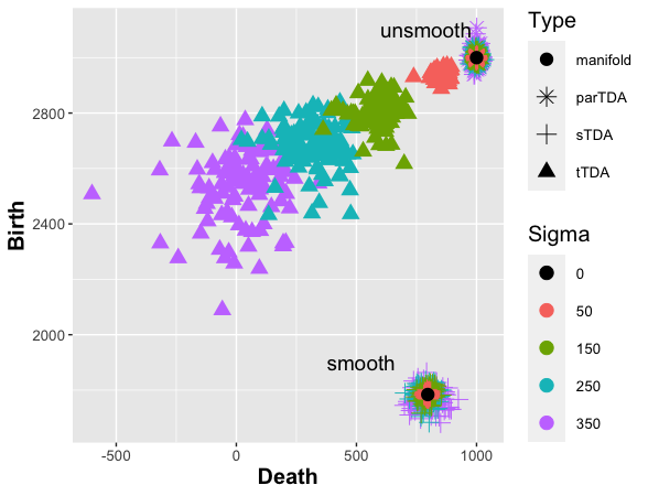
(a) (Death, Birth) of loop

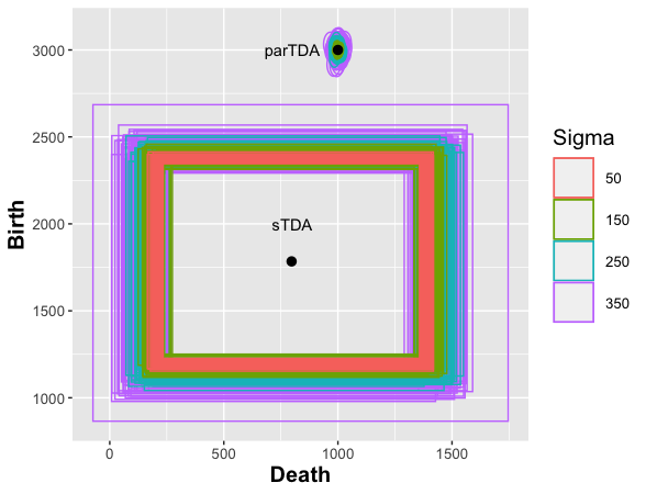
(b) Confidence Regions

Figure 6: Birth and death estimates (a) and confidence regions (b) of 100 images across four noise levels, $\sigma=\{50,150,250,350\}$. (a) Point estimates for $(\mu_{1*},\mu_{1})$ using tTDA (triangle) and parTDA (asterisk), estimates of $(\tilde{\mu}_{1*},\tilde{\mu}_{1})$ using sTDA (plus), and the true birth and death time of the manifold (circle). (b) The $95$% confidence regions for $(\mu_{1*},\mu_{1})$ using parTDA and $(\tilde{\mu}_{1*},\tilde{\mu}_{1})$ using sTDA.

Across all noise settings, point estimates from tTDA in Figure 6(a) are significantly biased, especially as the noise level increases. While parTDA creates unbiased estimates close to $\mu_{1*}$ and $\mu_{1}$ and sTDA creates unbiased estimates close to $\tilde{\mu}_{1*}$ and $\tilde{\mu}_{1}$. However, the confidence regions created using parTDA are much smaller (more precise) compared to sTDA. Using sTDA, the confidence bands are large enough that a persistence of zero is within each confidence region for every loop in the data. This result suggests that no loop is distinctly identified within the underlying pattern. Whereas, parTDA correctly identifies one loop for all simulated images when using Algorithm 1, and no other loops in the image are matched to the segmentation. In terms of coverage, sTDA covers the true birth and death times of $\mathcal{\tilde{M}}^{0}$ $100$% of the time for a $95$% confidence region. In comparison, the coverage of parTDA was always approximately $95$% at all noise levels.

Method	Noise Level	Average confidence region area (SE)	Average coverage (SE)
sTDA	50	1390574 (5553.5)	100 (0)
	150	1460183 (9529.5)	100 (0)
	250	1577603 (14139.8)	100 (0)
	350	1746974 (28184.4)	100 (0)
parTDA	50	122.9 (0.683)	94.7 (0.2)
	150	1099.3 (7.732)	95.3 (0.2)
	250	3057.2 (18.359)	94.6 (0.2)
	350	5980.2(30.602)	94.9 (0.3)

Table 1: Simulations Results of a noisy loop for sTDA (rows 1-4) and parTDA (rows 5-8). The average confidence region area and standard errors (SE) are displayed for each noise level, based on 100 iid images in each setting. The fourth column is the percent coverage of the 95% confidence regions, and corresponding SEs.

5 Cell Biology Application

Pattern formation is a common and critically important feature of living systems. It is a natural process that occurs across biological scales ranging from ecosystems (Pringle and Tarnita, 2017; Barbier et al., 2022), to developing tissues (Madamanchi et al., 2021; Herron et al., 2022), to individual cells (Bement et al., 2022, 2024). Further, abnormal cell or tissue pattern formation is a feature of various pathological conditions, including cancers (Paine and Lewis, 2017; A., 2020). Consequently, approaches for objectively detecting and quantifying patterns and their quality are of interest for both basic biology and medicine. In this paper, pattern is assessed from the perspective of TDA through estimation of the birth and death times of rings with parTDA. A higher persistence (birth-death) is indicative of stronger topological signal, and can be interpreted as a stronger pattern in this context.

The proposed parTDA is applied to images of two individual cells sustaining wounds at distinct time points as illustrated in Figure 7. One of the cells was injected with a toxin (C3 exotransferase) that inhibits healing. The other cell is only wounded with no injection and serves as a control. The image for the C3 cell is denoted as $\mathcal{M}^{\text{c3}}_{t}$ and the image for the Control cell denoted as $\mathcal{M}^{\text{control}}_{t}$ for times $t=\{t_{1},\ldots,t_{30}\}$. Time $t_{1}=0$ seconds is when the cell is wounded with sequential images separated by 8 seconds. Examples of the cell images at different time points are shown in Figure 7(a). Each of the images at every time point, $\mathcal{M}^{\text{control}}_{t}$ and $\mathcal{M}^{\text{c3}}_{t}$, was partitioned using the segmentation scheme from Section 3.4 with $e^{\text{control}}_{t}$ and $e^{\text{c3}}_{t}$ representing the edge sets at time $t$. An example of a segmentation at $t_{15}$ for $\mathcal{M}^{\text{c3}}_{t}$ is shown in Figure 7(b).

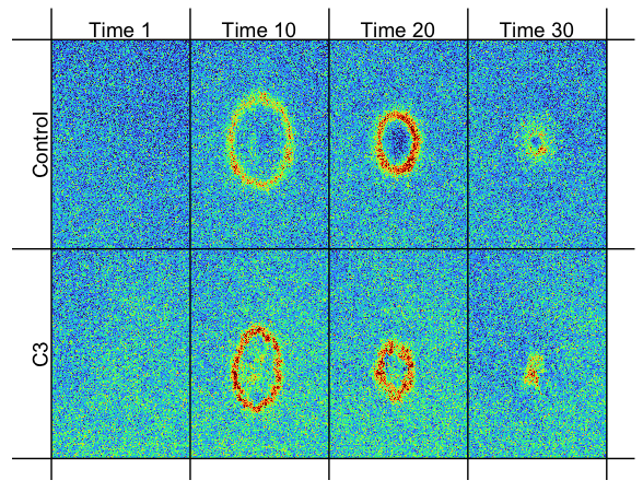
(a) $\mathcal{M}^{\text{control}}_{t}$ and $\mathcal{M}^{\text{c3}}_{t}$ for $t=\{t_{1},t_{10},t_{20},t_{30}\}$

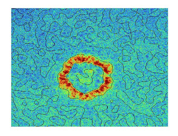
(b) Segmentation $e^{\text{c3}}_{t_{15}}$

Figure 7: (a) The top row displays the images for the control cell $\mathcal{M}^{\text{control}}_{t}$ and the bottom row is the images for the C3 cell $\mathcal{M}^{\text{c3}}_{t}$. The columns represent different time points, $t_{1}$, $t_{10}$, $t_{20}$, and $t_{30}$. (b) Image of $\mathcal{M}^{\text{c3}}_{t_{15}}$ segmented by $e^{\text{c3}}_{15}$ where the black lines are the edges.

The analysis is conducted independently at each time point. For each $t$ the number of rings in an image are detected using Algorithm 1 and a confidence region is created around the birth and death times using Equation 4. In this higher resolution image, Algorithm 1 has to be modified because multiple pixels in the image are equal to $b_{j}$. To address this, we smoothed the image, calculated the birth and death times, and used the smoothed birth time $\tilde{b}_{j}$ to help locate the pixel associated with $b_{j}$.

For both $\mathcal{M}^{\text{c3}}$ and $\mathcal{M}^{\text{control}}$, no ring was detected until time $t_{8}$ for the parTDA method even though the tTDA method does detect rings in images for $t\leq t_{7}$. When using parTDA no ring was contained in $e^{\text{control}}_{t}$ and $e^{\text{c3}}_{t}$ for $t\leq t_{7}$, so Algorithm 1 has no partitions to match with the rings detected in tTDA. From times $t_{8}$ to $t_{28}$ one ring is matched from $e^{\text{control}}_{t}$ to $\mathcal{M}^{\text{control}}_{t}$ and from $e^{\text{c3}}_{t}$ to $\mathcal{M}^{\text{c3}}_{t}$ using parTDA and thus these are the times focused on in this section.

Two different visualizations of persistence across time for both cells are displayed in Figure 8. In Figure 8(a), the parTDA birth and death estimates are shown on a persistence diagram along with the confidence regions. The estimated birth and death times are connected by time, where time is indicated by different colors. Figure 8(b), is another way to visualize persistence (y-axis) over time (x-axis). When using parTDA, the estimated persistence is $\bar{Z}^{1}_{t}-\bar{Z}^{1*}_{t}$, at each time $t$. The confidence set moves from a bivariate normal ellipse to a normal confidence interval centered at $\bar{Z}^{1}_{t}-\bar{Z}^{1*}_{t}$ with approximate variance $(\hat{\sigma}^{2}_{1})_{t}+(\hat{\sigma}^{2}_{1*})_{t}$. The red lines are the estimated persistence and confidence intervals from parTDA for both C3 (points) and Control (triangle) cells; the error bars are too small too see since sample size is large due to the high-resolution images. The dark blue lines use sTDA and the light blue lines use tTDA to estimate persistence across time; no confidence intervals were created for these methods. In general, sTDA and tTDA display more variability in the estimated persistences across time than parTDA, and the C3 and Control cell persistences for tTDA are not well separated. The overall trends in sTDA and parTDA are similar, though the parTDA persistences appear to be more stable across time.

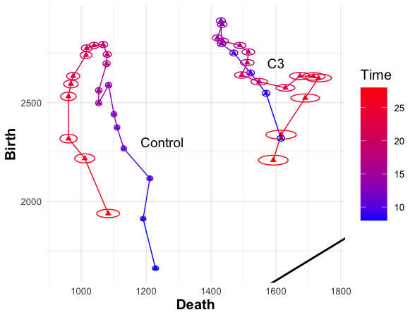
(a) (Death, Birth) estimates

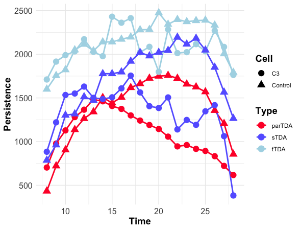
(b) Estimated Persistence

Figure 8: Estimated persistences of the C3 and Control cell images from $t=\{t_{8},\ldots,t_{28}\}$. (a) The parTDA birth and death times are shown on the persistence diagram along with confidence regions for both the C3 cell (right) and the Control cell (left). The black line is the diagonal line $b=d$. (b) Persistence is plotted over time for the C3 cell (solid line with points) and the Control cell (dashed line with triangles) using parTDA (red), sTDA (purple), and tTDA (light blue).

From $t_{8}$ to $t_{14}$, the most rapid growth in the persistence (or strength of pattern) are observed. Originally, the C3 cell images have more pattern in terms of the ring having a higher persistence than the Control cell images. However, at $t_{14}$ the wound ring in the Control cell continues to increase in its persistence while the wound ring in C3 cell begins to decline. In later time periods, the rings have shrunk in size, but not necessarily in intensity. The smaller size of the rings in the images result in larger confidence regions since the sample sizes of the sample means (i.e., the number of pixels in the pattern) has decreased. After $t_{29}$ the segmentation, $e^{\text{c3}}_{t_{29}}$, does not have any rings in the partitions; the edge set in the background is almost completely connected as one edge. Two distinct edges are needed to separate the section of an image into $\mathcal{M}^{\sigma}_{i}$ and $\mathcal{M}^{\sigma}_{i*}$ to find a ring in the segmentation. Therefore, no ring on $\mathcal{P}(\mathcal{M}^{\text{c3}}_{29})$ is matched to any regions in $e^{\text{c3}}_{t_{29}}$ as per Algorithm 1.

During times $t_{29}-t_{30}$, the segmentation of the Control cell images continues to detect a ring where the wound is (i.e., two distinct edges separate $\mathcal{M}^{\text{Control}}_{1}$ and $\mathcal{M}^{\text{Control}}_{1*}$ which are matched to the ring detected in $\mathcal{P}(\mathcal{M}^{\text{Control}})$ for times $t_{29},t_{30}$); however, in order to directly compare the Control cell with the C3 cell only times $t_{8}-t_{28}$ are included in Figure 8.

6 Conclusions and Discussions

This paper includes three primary developments in TDA methodology. First, parTDA is proposed to estimate the birth and death times of topological features found in an image, which reduces the bias in the traditional TDA estimates (tTDA). Second, parTDA provides a process to quantify the uncertainty associated with these new birth and death time estimates in the form of a confidence region on a persistence diagram for an image. And finally, a persistence diagram confidence region method of Fasy et al. (2014) was extended from point-cloud data to a single image as an alternative method (sTDA), which facilitated the creation of a new method to bootstrap an image. In general, parTDA is applicable to any image to determine the underlying pattern (in terms of holes) of that image and to quantify the uncertainty in that pattern.

Our novel parTDA approach builds confidence regions on topological summary statistics (persistence diagrams) through estimating the mean and variance of the partitions associated with the birth and death times of homology group generators in the image. These estimated means and variances use the Central Limit Theorem to get confidence ellipses for the birth and death times of loops in the persistence diagram. The sample means of pixels within the estimated birth and death time partitions of the manifold are represented on the persistence diagram through a matching procedure between parTDA and tTDA using Algorithm 1. The parTDA confidence regions are more accurate in terms of coverage and have a smaller area than the alternative method, sTDA.

The proposed methods were motivated by a cell biology application. parTDA was able to detect a pattern which distinguishes the wounded C3 cell from the wounded Control cell through differences in persistence over time with no overlapping confidence regions. The confidence regions are the main result which are useful to biologists to quantify the uncertainty in the ring structures in the images. We are interested in seeing if the differences in the persistence over time is consistent when looking at more images of different cells. Furthermore, it is of interest to more directly include time into the TDA analysis, through connecting loops across time and estimating the temporal uncertainty of the pattern. With these extensions, further investigation may be done to try and understand the mechanism at work when a cell is wounded under normal versus pathological conditions.

For future research, we aim to extend the parTDA framework to include time and continuous functions or point-cloud data settings. An extension of parTDA to point-cloud data can be directly compared to the methods of Fasy et al. (2014). In Section 4, sTDA uses the $L_{\infty}$ distance between images to estimate the confidence regions as opposed to the bottleneck distance between persistence diagrams to be consistent with the Fasy et al. (2014) approach. The confidence regions are smaller using the bottleneck distance (though still significantly larger than the parTDA confidence regions), but the coverage is still at $100\%$. We are interested in investigating why these confidence regions are large for both the point cloud and image settings.

Another possible direction is to add a probabilistic element to the image segmentation, such as fuzzy clustering, to reduce false positive loops detected in the pattern. For instance, the segmentation may introduce a loop that is not part of the underlying pattern but is also matched to a loop found using tTDA. While parTDA is designed to build confidence regions, they can also be applicable to hypothesis testing to separate topological signal from noise. The performance of parTDA as a hypothesis testing framework is a topic of future investigation.

References

- A. [2020] U. A. Cancer: A turbulence problem. Neoplasia, 22(12):759–769, 2020. doi: 10.1016/j.neo.2020.09.008.
- Barbier et al. [2022] I. Barbier, H. Kusumawardhani, and Y. Schaerli. Engineering synthetic spatial patterns in microbial populations and communities. Current Opinion in Microbiology, 67, 2022. doi: 10.1016/j.mib.2022.102149.
- Bement et al. [2022] W. M. Bement, A. L. Miller, and G. von Dassow. Rho GTPase activity zones and transient contractile arrays. Bioessays, 28(10):983–93, 2022. doi: 10.1002/bies.20477.
- Bement et al. [2024] W. M. Bement, A. B. Goryachev, A. L. Miller, and G. von Dassow. Patterning of the cell cortex by rho GTPases. Nat Rev Mol Cell Biol, 25:290–308, 2024. doi: 10.1038/s41580-023-00682-z.
- Bukkuri et al. [2021] A. Bukkuri, N. Andor, and I. Darcy. Applications of topological data analysis in oncology. Frontiers in Artificial Intelligence, 4:659037, 04 2021. doi: 10.3389/frai.2021.659037.
- Burkel et al. [2012] B. M. Burkel, H. A. Benink, E. M. Vaughan, G. von Dassow, and W. M. Bement. A rho GTPase signal treadmill backs a contractile array. Developmental cell, 23(2):384–396, 2012.
- Canny [1986] J. F. Canny. A computational approach to edge detection. IEEE Transactions on Pattern Analysis and Machine Intelligence, PAMI-8:679–698, 1986. URL https://api.semanticscholar.org/CorpusID:13284142.
- Chazal and Michel [2021] F. Chazal and B. Michel. An introduction to topological data analysis: Fundamental and practical aspects for data scientists. Frontiers in Artificial Intelligence, 4, 2021. doi: 10.3389/frai.2021.667963.
- Chung et al. [2009] M. K. Chung, P. Bubenik, and P. T. Kim. Persistence diagrams of cortical surface data. In Information Processing in Medical Imaging, 21st International Conference, IPMI 2009, Williamsburg, VA, USA, July 5-10, 2009. Proceedings, volume 5636 of Lecture Notes in Computer Science, pages 386–397. Springer, 2009. ISBN 978-3-642-02497-9. doi: 10.1007/978-3-642-02498-6˙32.
- Cohen-Steiner et al. [2005] D. Cohen-Steiner, H. Edelsbrunner, and J. Harer. Stability of persistence diagrams. volume 37, pages 263–271, 01 2005. doi: 10.1007/s00454-006-1276-5.
- Edelsbrunner and Harer [2010] H. Edelsbrunner and J. Harer. Computational Topology - an Introduction. American Mathematical Society, 2010. ISBN 978-0-8218-4925-5.
- Fasy et al. [2014] B. T. Fasy, F. Lecci, A. Rinaldo, L. Wasserman, S. Balakrishnan, and A. Singh. Confidence sets for persistence diagrams. The Annals of Statistics, 42(6), dec 2014. doi: 10.1214/14-aos1252. URL https://doi.org/10.1214%2F14-aos1252.
- Gupta et al. [2023] S. Gupta, Y. Zhang, X. Hu, P. Prasanna, and C. Chen. Topology-aware uncertainty for image segmentation, 2023.
- Haglund et al. [2019] K. Haglund, I. P. Nezis, and H. Stenmark. Structure and functions of stable intercellular bridges formed by incomplete cytokinesis during development. Communicative & Integrative Biology, 4(1):1–9, 2019. doi: 10.4161/cib.13550.
- Herron et al. [2022] J. C. Herron, S. Hu, B. Liu, T. Watanabe, K. M. Hahn, and T. C. Elston. Spatial models of pattern formation during phagocytosis. PLOS Computational Biology, 18, 10 2022. doi: 10.1371/journal.pcbi.1010092.
- Madamanchi et al. [2021] A. Madamanchi, M. C. Mullins, and D. M. Umulis. Diversity and robustness of bone morphogenetic protein pattern formation. Development, 148(7), 2021. doi: 10.1242/dev.192344.
- Mandato and Bement [2001] C. A. Mandato and W. M. Bement. Contraction and polymerization cooperate to assemble and close actomyosin rings around xenopus oocyte wounds. The Journal of Cell Biology, 154:785 – 798, 2001. URL https://api.semanticscholar.org/CorpusID:481388.
- Mileyko et al. [2011] Y. Mileyko, S. Mukherjee, and J. Harer. Probability measures on the space of persistence diagrams. Inverse Problems, 27(12):124007, nov 2011. doi: 10.1088/0266-5611/27/12/124007. URL https://doi.org/10.1088/0266-5611/27/12/124007.
- Otter et al. [2017] N. Otter, M. A. Porter, U. Tillmann, P. Grindrod, and H. A. Harrington. A roadmap for the computation of persistent homology. EPJ Data Science, 6(1), aug 2017. doi: 10.1140/epjds/s13688-017-0109-5. URL https://doi.org/10.1140%2Fepjds%2Fs13688-017-0109-5.
- Paine and Lewis [2017] I. Paine and M. Lewis. The terminal end bud: the little engine that could. J Mammary Gland Biol Neoplasia, 22:93–108, 2017. URL https://doi-org.ezproxy.library.wisc.edu/10.1007/s10911-017-9372-0.
- Parker [2010] J. R. Parker. Algorithms for Image Processing and Computer Vision. John Wiley & Sons, Inc., New York, 2010.
- Pollard and O’Shaughnessy [2019] T. D. Pollard and B. O’Shaughnessy. Molecular mechanism of cytokinesis. Annual Review of Biochemistry, 88(1):661–689, 2019. doi: 10.1146/annurev-biochem-062917-012530.
- Pringle and Tarnita [2017] R. M. Pringle and C. E. Tarnita. Spatial self-organization of ecosystems: Integrating multiple mechanisms of regular-pattern formation. Annual Review of Entomology, 62(1):359–377, 2017. doi: 10.1146/annurev-ento-031616-035413.
- Singh et al. [2023] Y. Singh, C. M. Farrelly, Q. A. Hathaway, T. Leiner, J. Jagtap, u. E. Carlsson, and B. J. Erickson. Topological data analysis in medical imaging: current state of the art. Insights Imaging, 14(58), 2023. doi: 10.1186/s13244-023-01413-w.
- Skaf and Laubenbacher [2022] Y. Skaf and R. Laubenbacher. Topological data analysis in biomedicine: A review. Journal of Biomedical Informatics, 130:104082, 05 2022. doi: 10.1016/j.jbi.2022.104082.
- Turner et al. [2014] K. Turner, Y. Mileyko, S. Mukherjee, and J. Harer. Fréchet means for distributions of persistence diagrams. Discrete & Computational Geometry, 52(1):44–70, 2014.
- Wang et al. [2023] J. Wang, K. Meng, and F. Duan. Hypothesis testing for medical imaging analysis via the smooth euler characteristic transform. 08 2023.