Investigating the Cosmological Rate of Compact Object Mergers from Isolated Massive Binary Stars

Abstract

Gravitational wave detectors are observing compact object mergers from increasingly far distances, revealing the redshift evolution of the binary black hole (BBH)—and soon the black hole-neutron star (BHNS) and binary neutron star (BNS)—merger rate. To help interpret these observations, we investigate the expected redshift evolution of the compact object merger rate from the isolated binary evolution channel. We present a publicly available catalog of compact object mergers and their accompanying cosmological merger rates from population synthesis simulations conducted with the COMPAS software. To explore the impact of uncertainties in stellar and binary evolution, our simulations use two-parameter grids of binary evolution models that vary the common-envelope efficiency with mass transfer accretion efficiency, and supernova remnant mass prescription with supernova natal kick velocity, respectively. We quantify the redshift evolution of our simulated merger rates using the local ($z\sim 0$) rate, the redshift at which the merger rate peaks, and the normalized differential rates (as a proxy for slope). We find that although the local rates span a range of $\sim 10^{3}$ across our model variations, their redshift-evolutions are remarkably similar for BBHs, BHNSs, and BNSs, with differentials typically within a factor $3$ and peaks of $z\approx 1.2-2.4$ across models. Furthermore, several trends in our simulated rates are correlated with the model parameters we explore. We conclude that future observations of the redshift evolution of the compact object merger rate can help constrain binary models for stellar evolution and gravitational-wave formation channels.

1 Introduction

Observations of gravitational waves from compact object mergers are revolutionizing our understanding of stellar mass black holes and neutron stars across cosmic time. To date, data taken with the detector network consisting of Advanced LIGO (Aasi et al., 2015) Advanced Virgo (Acernese et al., 2015), and KAGRA (Akutsu et al., 2021) include on the order of $100$ statistically significant GW observations of binary black holes out to redshifts $z\sim 1.5$ (e.g., Abbott et al., 2023; Nitz et al., 2023; Venumadhav et al., 2019, 2020; Zackay et al., 2019; Olsen et al., 2022; Mehta et al., 2023; Wadekar et al., 2023). These observations already probe the BBH merger rate as a function of redshift (e.g., Abbott et al., 2021; Nitz et al., 2023; Callister & Farr, 2023; Payne & Thrane, 2023; Ray et al., 2023), and future observing runs equipped with technological upgrades such as O4, O5, and $A^{\#}$ are expected to increase the detection volume for stellar mass BBHs out to redshift $z\sim 2$ (e.g., Baibhav et al., 2019; Adhikari et al., 2020; Gupta et al., 2023). Moreover, next-generation detectors like the Einstein Telescope and Cosmic Explorer are expected to make $\gtrsim 100,000$ detections annually from binary neutron star (BNS) and black hole–neutron star (BHNS) mergers out to redshifts $z\gtrsim 2$ and BBH mergers out to redshift $\gtrsim 10$. The observational capacities of these detectors will allow us to measure the redshift distribution of mergers to within percent level precision (Punturo et al., 2010; Sathyaprakash et al., 2012; Maggiore et al., 2020; Reitze et al., 2019; Evans et al., 2021; Borhanian & Sathyaprakash, 2022; Iacovelli et al., 2022; Singh et al., 2022; Gupta et al., 2023).

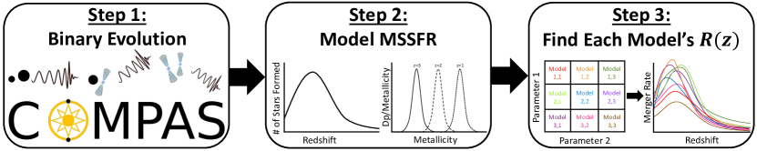
Figure 1: Schematic overview of the method used in this paper. Step 1: Simulate the evolution of binaries with each combination of parameters from the two-parameter grids (Table 1) using the COMPAS binary population synthesis code. Step 2: Distribute binaries from simulations across redshift using a metallicity-specific star formation rate. Step 3: Infer the BBH, BHNS, and BNS merger rates from the simulation results of each parameter combination in the two-parameter grids.

To realize the full potential of these GW observations, we use theoretical models of binary evolution to infer their formation channels and learn about the underlying physical processes that lead to compact object mergers (e.g., Zevin et al., 2021; Mapelli, 2021; Mandel & Farmer, 2022). Thus far, the majority of literature has attempted to compare simulated merger rates to the observed local ($z\sim 0$) merger rates, but the local rates alone do not provide enough information to distinguish formation pathway contributions due to the many poorly-constrained parameters in population synthesis simulations (Mandel & Broekgaarden, 2022). There has therefore been increasing interest in investigating the properties and rates of double compact object (DCO) mergers as a function of redshift because of the information that they encode about formation channels (e.g., Ng et al., 2021; Zevin et al., 2021; Singh et al., 2022; van Son et al., 2022).

To explore the cosmological merger rates, this study investigates the redshift distribution of DCO mergers created by the isolated binary evolution channel, in which GW sources form from pairs of massive stars. Our analysis is more in depth than most previous studies in three ways: (i) we analyze the BBH, BHNS, and BNS merger rates simultaneously, (ii) we explore the impact of uncertain populations synthesis parameters in tandem using two grids of simulations with varying assumptions for the mass transfer, common envelope, and supernova physics, and (iii) we calculate summary statistics, such as the ‘differential merger rates’ across several redshift bins to efficiently analyze the impact of different massive binary evolution uncertainties on the expected distribution of mergers. Our simulations are publicly available at https://gwlandscape.org.au/compas/.

2 Methods

We calculate the merger rates of simulated BBH, BHNS, and BNS systems formed by isolated massive binary stars in a three-step process shown in Figure 1 and summarized below.

Table 1: Overview of the models explored in this study. For the remnant mass prescriptions we use the ‘delayed’ and ‘rapid’ prescriptions from Fryer et al. (2012) and the ‘stochastic’ prescription from Mandel & Müller (2020).

Grid label (dimensions)	Parameters	Values	Changed physics
A (4x3)	$\alpha_{\rm{CE}}$	$[0.1,0.5,2.0,10.0]$	Common envelope ejection efficiency
	$\beta$	$[0.25,0.5,0.75]$	Mass transfer accretion efficiency
B (3x3)	Supernova	[delayed, rapid, Mandel & Müller]	SN remnant mass prescription
	$\sigma_{\rm{rms}}^{\rm{1D}}$	$[30,265,750]\,\rm{km}\ \rm{s}^{-1}$	1d rms natal kick velocity

2.1 Population Synthesis Simulations

We use the COMPAS suite to rapidly evolve large populations of stellar binaries, a fraction of which create compact objects and merge (Team COMPAS: Riley et al., 2022). COMPAS is built on the single star evolution analytic fitting formulae by Hurley et al. (2000, 2002) which are based on single star evolution tables from Pols et al. (1998) and earlier work from Eggleton et al. (1989) and Tout et al. (1996); it parameterizes and approximates stellar evolution and binary interaction in order to rapidly ($\lesssim 1$ sec) compute the evolution of binary systems. We ran population synthesis simulations over two dimensional grids of model parameters to explore the correlated impact of binary physics uncertainties. We created two grids, which we will refer to as grid A and grid B, and which we summarize below and in Table 1.

In grid A, we vary common envelope (CE) efficiency and mass transfer efficiency. These two parameters are of interest because they have been the focus of several prior studies, are highly uncertain, and have been demonstrated to significantly impact populations synthesis outcomes (Vigna-Gómez et al., 2018; Bavera et al., 2021; Dorozsmai & Toonen, 2024; Santoliquido et al., 2021; Broekgaarden et al., 2022). CE phases are defined by dynamically unstable mass transfer in which on of the companions’ envelope engulfs the other, causing drag and tightening the binary. COMPAS parameterizes the CE phase with the ‘$\alpha_{\rm{CE}}-\lambda$’ formalism (introduced by Webbink (1984) and de Kool (1990)), where $\alpha_{\rm{CE}}$ determines the fraction of orbital energy that binaries expend to eject their CEs. For grid A we choose a range of values representative of the literature: $\alpha_{\rm{CE}}=0.1,\ 0.5,\ 2.0,\textrm{ and }10.0$ (Santoliquido et al., 2022; Broekgaarden et al., 2021; Neijssel et al., 2019; van Son et al., 2022), and we fix $\lambda$ to $\lambda_{\textrm{Nanjing}}$ from the fit in Xu & Li (2010a, b). The mass transfer efficiency parameter is $\beta=\Delta M_{\rm acc}/M_{\rm donor}$ where $\Delta M_{\rm donor}$ and $\Delta M_{\rm acc}$ are the changes in the mass of the donor and accretor stars, respectively, during stable transfer. We use three values, $\beta=0.25,\ 0.5$, and $0.75$.

In grid B, we vary the core collapse supernovae (CCSNe) natal kick velocity and the supernova (SN) remnant mass prescription (RMP). Our simulations give supernovae (SNe) a kick with velocity $v_{k}$ drawn from a Maxwell-Boltzman distribution with dispersion $\sigma_{\rm{rms}}^{\rm{1D}}$. We explore $\sigma_{\rm{rms}}^{\rm{1D}}=30,\ 265,\textrm{ and }750\ \textrm{km s}^{-1}$ for CCSNe. Higher dispersion leads to faster kicks, which studies have found to be proportional to the amount of ejecta from SNe. We therefore choose these dispersion values to approximate having weak kicks ($\sigma_{\rm{rms}}^{\rm{1D}}=30$), commonly-used moderate kicks ($\sigma_{\rm{rms}}^{\rm{1D}}=265$ from Hobbs et al. (2005)), and strong kicks ($\sigma_{\rm{rms}}^{\rm{1D}}=750$). RMP maps objects’ carbon-oxygen core mass to a remnant mass after SN, and is largely responsible for determining if stars become NSs or BHs. In grid B, we adopt three RMPs for CCSNe: “delayed” (Fryer et al., 2012), “rapid” (Fryer et al., 2012), and “stochastic” (Mandel & Müller, 2020). The rapid prescription assumes that SN explosions occur within $250$ ms as opposed to the longer duration in the delayed model; the rapid model reproduces a mass gap between NSs and BHs . The “stochastic” model, on the other hand, enables NS and BH formation in multiple regions of the parameter space. Kick velocity is associated with mass ejecta, which in turn reduces the remnant mass as remnants accumulate ejecta through "fallback" driven by their gravitational pull.

For each pairing of parameter values in our grids, we evolve $20$ million binaries with initial stellar masses drawn from the Kroupa (2001) initial mass function in the $5-150\,\rm{M}_{\odot}$ range. For all parameters not varied by the grids in this study, we use the default values from COMPAS (Team COMPAS: Riley et al., 2022) which are listed in appendix Table 2.

2.2 Calculating the Merger Rate

We calculate the cosmological merger rates of compact objects following the methodology in Team COMPAS: Riley et al. (2022). The merger rate measured by a comoving observer at a merger time $t_{m}$ since the Big Bang for a binary consisting of components with masses $M_{1},$ and $M_{2}$ is

$$\begin{split}&\mathcal{R}_{\rm{merge}}(t_{m},M_{1},M_{1})\equiv\frac{\textrm{d}^{4}N_{\textrm{merge}}}{\textrm{d}t_{m}\textrm{d}V_{c}\textrm{d}M_{1}\textrm{d}M_{2}}(t_{\textrm{m}},M_{1},M_{2})\\ &=\int\textrm{d}Z_{i}\int_{0}^{t_{m}}\textrm{d}t_{\textrm{delay}}\mathcal{S}(Z_{i},z(t_{\textrm{form}}=t_{m}-t_{\textrm{delay}}))\times\\ &\frac{\textrm{d}^{4}N_{\textrm{form}}}{\textrm{d}M_{\textrm{SFR}}\textrm{d}t_{\textrm{delay}}\textrm{d}M_{1}\textrm{d}M_{2}}(Z_{i},t_{\textrm{delay}},M_{1},M_{2}),\end{split}$$ (1)

where $N_{\rm{merger}}$ is the number of systems merged, $N_{\rm{form}}$ is the number of systems formed, $V_{c}$ is the comoving volume, $t_{\textrm{delay}}$ is the time between the formation and merger of the binary, $Z_{i}$ is the birth metallicity of the components, $M_{\rm{SFR}}$ is a unit of star forming mass, and we convolve the metallicity-specific star formation rate density $\mathcal{S}(Z_{i},z(t_{\textrm{form}}))$ with the formation yield.

2.3 Metallicity-Specific Star Formation History

In order to model $S(Z_{i},z(t_{\rm{form}}))$, which describes star formation history as a function of initial redshift and metallicity, we follow Team COMPAS: Riley et al. (2022); Broekgaarden et al. (2019): we multiply the star formation rate density (SFRD) by a metallicity probability density function

$$\begin{split}\mathcal{S}(Z_{i},z_{form})&=\frac{\textrm{d}^{3}M_{\textrm{SFR}}}{\textrm{d}t_{s}\textrm{d}V_{c}\textrm{d}Z_{i}}(z_{form})\\ &=\frac{\textrm{d}^{2}M_{\rm{SFR}}}{\textrm{d}t_{s}\textrm{d}V_{c}}(z_{form})\times\frac{\textrm{d}P}{\textrm{d}Z_{i}}(z_{form})\end{split}$$ (2)

where $z_{\rm{form}}$ is the redshift at which DCOs form and $t_{s}$ is the time in the merger’s source frame. We obtain the metallicity density function $\frac{\textrm{d}P}{\textrm{d}Z_{i}}(z_{\rm{form}})$ by convolving the number density of galaxies per logarithmic mass bin (GSMF) and the mass-metallicity relation.

For this study we use the SFRD fit from Madau & Fragos (2017), which is an update from the earlier work Madau & Dickinson (2014). We adopt the GSMF from Panter et al. (2004) which is a standard Schechter fit based on the Sloan Digital Sky Survey data. We use the MZR from Ma et al. (2016), which was derived using high-resolution cosmological zoom-in simulations from (Hopkins et al., 2014). Models for $S(Z,z)$ are another source of high uncertainty which impacts merger rate approximation (Chruślińska, 2022; Broekgaarden et al., 2022; van Son et al., 2022). Evaluating the impact of the SFRD on the merger rate will be a substantial effort that we leave for future studies.

2.4 Quantifying the Merger Rate Redshift Evolution

To understand how parameter variations impact the redshift evolution of the merger rate, it is helpful to use summary statistics for the $z$-distribution and behavior of $\mathcal{R}_{\rm{merge}}(z)$. We quantify the merger rate $z$-evolution by calculating the relative differential rates

$$\frac{\Delta\mathcal{R}_{\rm{merge}}}{\Delta z}(z_{\rm{min}},z_{\rm{max}})=\frac{\mathcal{R}_{\rm{m}}(z_{\rm{max}})-\mathcal{R}_{\rm{m}}(z_{\rm{min}})}{(z_{\rm{max}}-z_{\rm{min}})\int_{0}^{\infty}\mathcal{R}_{\rm{m}}(z)dz}$$ (3)

where $\mathcal{R}_{\rm{m}}(z)$ is shorthand for $\mathcal{R}_{\rm{merge}}(z)$, $z_{\rm{min}}$ and $z_{\rm{max}}$ set the bounds for the differential rate, and the integral in the denominator is used to scale the rates such that the differential values describe redshift evolution instead of the number of mergers. We choose this metric because it represents the slopes (relative increase) of the merger rate for a given redshift bin.

In this study, we calculate the differentials for the redshift ranges $[0,1]$, $[1,z_{\rm{peak}}]$, $[z_{\rm{peak}},z_{\rm{peak}}+1]$, $[z_{\rm{peak}}+1,9]$, where $z_{\rm{peak}}$ is the redshift of the peak. We select these ranges because (i) our rates monotonically increase and then decrease before and after the peak, respectively, (ii) it allows for breaks in the slope before and after the peak (as has been suggested by observational studies such as Callister & Farr (2023); Payne & Thrane (2023)), and (iii) the slope of $\mathcal{R}_{\rm{merge}}(z)$ far from the peak is highly-linear. When we discuss the redshift evolution of the merger rate in Section 3, we discuss the differentials as well as the intrinsic merger rate, $\mathcal{R}_{0}\equiv\mathcal{R}_{\rm{merge}}(0)$, and the redshift of the merger rate peak, $z_{\rm{peak}}$.

3 Results

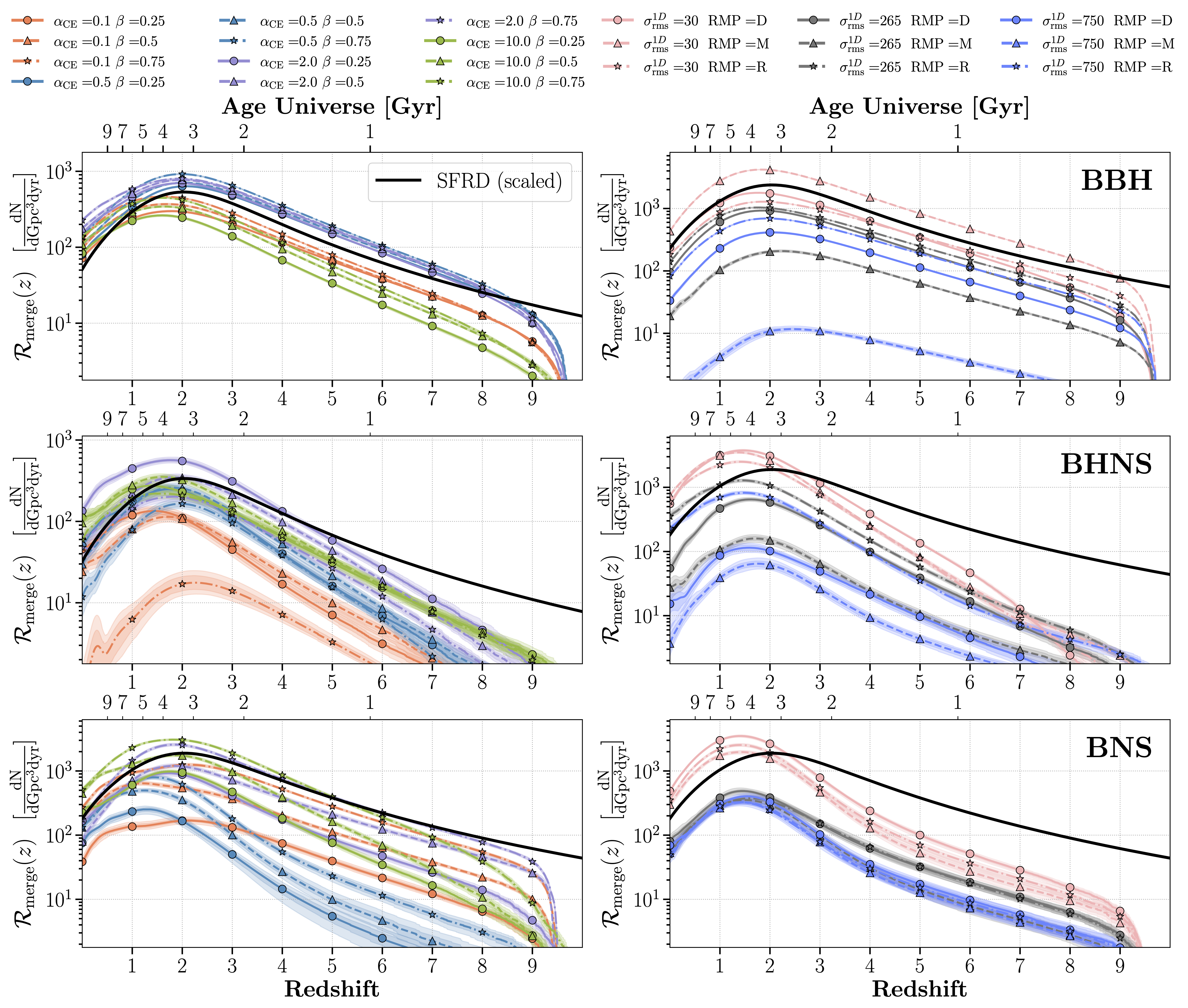
Figure 2: The BBH (top), BHNS (middle), and BNS (bottom) merger rates as a function of redshift for our simulations. The left column shows models from grid A, where we vary the common-envelope efficiency $\alpha_{\rm{CE}}$ and stable mass transfer efficiency $\beta$, and the right column shows models from grid B, where we vary the supernova natal kick velocity root-mean-square $\sigma_{\rm{rms}}^{\rm{1D}}$ and the remnant mass prescription (RMP). For the RMP prescription, D, M, and R stand for the delayed, Mandel & Müller (2020), and rapid prescription, respectively. The assumed SFRD from Madau & Fragos (2017) is scaled arbitrarily and plotted on all panels in black; note that the SFRD is, in reality, orders of magnitude greater than the merger rate but the scaling helps compare the shapes by eye. For all merger rates, we include the $1\sigma$ and $2\sigma$ confidence intervals calculated by bootstrapping the simulation results to show the sampling uncertainty. The sharp merger rate drop-off around $z\sim 9$ is due to our assumption that star formation starts at $z=10$ and mergers are delayed.

We show the simulated BBH, BHNS, and BNS merger rates as a function of redshift in Figure 2 for all binary evolution models. In Figure 3, we show a quantitative analysis of these rates’ redshift evolutions including their differential rates (defined in Equation 3), local rates, and peak redshifts. The differential rate is a representative of the “normalized” merger rate slope: values close to $1$ or $-1$ indicate steep increases or decreases whereas values close to 0 indicate flatter evolution over a given redshift interval. We will therefore refer to these differential rates as ‘slopes’. We find the following results.

Most importantly, we observe that the BBH, BHNS, and BNS merger rates follow a remarkably similar evolution over redshift for all our models: the merger rates rise monotonically between $z=0$ until their peaks between $1.5\lesssim z\lesssim 2.5$ and then steeply decline until $z\sim 9.5$ where they sharply drop off. In Figure 3 we show that the merger rates from all models peak between redshifts $1.60<z<2.40$ (BBH), $1.35\lesssim z\lesssim 2.26$ (BHNS), and $1.20\lesssim z\lesssim 2.13$ (BNS), and that their slopes typically vary with factors between $1$–$3\times$ for a given DCO type. The slopes that are outliers are (i) BNS models in the range $[1,z_{\rm{peak}}]$ which vary between $0.045$ and $0.22$ (a factor $4.8\times$) and (ii) BNS models in $[z_{\rm{peak}},z_{\rm{peak}}+1]$, which vary between $-0.26$ and $-0.06$ (a factor $4.3\times$). The redshift interval with the smallest variations in slope is $[z_{\rm{peak}}+1,9]$, for which values only span a factor of $1.1\times,1.2\times,$ and $1.2\times$ for BBHs, BHNSs, and BNSs, respectively. In contrast to the similarity of the merger distributions, we find that the intrinsic merger rates can span factors of almost $1000\times$ between models, namely $724\times$, $939\times$, and $13\times$ for BBH, BHNS, and BNS, respectively.

The merger rate slopes are so similar between models because the two primary factors that affect the redshift distribution of binaries are relatively model-agnostic. First, the formation efficiency as a function of metallicity follow the same general trend for a given DCO type with all of our models (see Figure 6 for the formation rates). Second, the delay time distribution of all models follow a $t^{-1}$–like distribution. Combined, these two effects govern the redshift distribution of mergers because they dictate where binaries form and how long they live before merging (see Boesky et al. 2024 for more details). In Figure 2, the BHNS merger rates have notably steeper slopes on average than BBHs for the range $z\gtrsim z_{\rm{peak}}$. This is a result of BHNSs having fewer systems with short delay times ($\lesssim 1\,\rm{Gyr}$), which we show in Figure 5, leading to fewer mergers at high redshift.

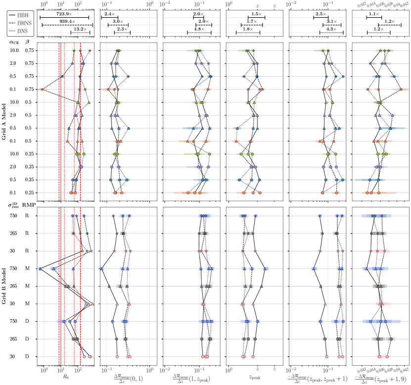
Figure 3: The intrinsic merger rate ($\mathcal{R}_{0}$), peak redshift ($z_{\rm{peak}}$), and merger rate differentials in the $z$ ranges $[0,1],[1,z_{\rm{peak}}],[z_{\rm{peak}},z_{\rm{peak}}+1],[z_{\rm{peak}}+1,9]$ for BBHs, BHNSs, BNSs. The top and bottom rows are for models in grid A and B, respectively, and colors and markers correspond to those in Figure 2. The red vertical lines in the first column are the inferred BBH, BHNS, and BNS local merger rates (90% credible intervals) from (Abbott et al., 2023). We include $1\sigma$ and $2\sigma$ confidence intervals as shaded boxes around each point, which are calculated by bootstrapping the simulation results. Along the y-axis in the left margin, RMP stands for remnant mass prescription and D, M, and R stand for the delayed, Mandel & Müller (2020), and rapid prescriptions, respectively.

We also notice several trends in how specific parameters impact the merger rates in Figures 2 and 3. The dominant parameter for the redshift distribution of mergers from grid A is the common envelope efficiency $\alpha_{\rm{CE}}$, as is visible by the clustering of rates by $\alpha_{\rm{CE}}$ in Figure 2. Models with $\alpha_{\rm{CE}}=0.1,10.0$ tend to produce fewer BBH mergers than models with $\alpha_{\rm{CE}}=0.5,2.0$. Our simulations are therefore consistent earlier studies which found that $\alpha_{\rm{CE}}$ has a non-monotonic effect on binary physics (e.g. Broekgaarden et al., 2022; Bavera et al., 2022). Models with $\alpha_{\rm{CE}}=0.1$ and $2.0$ produce the least BHNS mergers, whereas models with $\alpha_{\rm{CE}}=0.5$ and $0.1$ produce the least BNSs mergers, depending on the value of $\beta$. We also find that models with $\alpha_{\rm{CE}}=0.1,10.0$ tend to favor low redshift BBH mergers relative to other grid A models.

The SN natal kick velocity dispersion $\sigma_{\rm{rms}}^{\rm{1D}}$ dominates the redshift distribution of mergers for grid B. In Figure 2 we find that holding the remnant mass prescription constant, the number of mergers monotonically decreases (often with more than a factor $10\times$) with increasing $\sigma_{\rm{rms}}^{\rm{1D}}$. This is because higher $\sigma_{\rm{rms}}^{\rm{1D}}$ values lead more binaries to disrupt during supernova. The number of mergers span the largest range between $\sigma_{\rm{rms}}^{\rm{1D}}$ perscriptions for BBHs with the Mandel $\&$ Müller RMP, indicating that BBH simulations with this stochastic RMPs are particularly sensitive to $\sigma_{\rm{rms}}^{\rm{1D}}$.

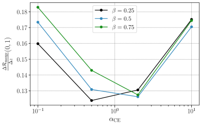
Figure 4: The differential BBH merger rate in the interval $z=0$ to $z=1$ as a function of $\alpha_{\rm{CE}}$ values for different fixed values of $\beta$ in our simualtion grid A.

Trends in how parameters impact the merger rate are often consistent across values for the second grid parameter. One example is the BBH slope as a function of $\alpha_{\rm{CE}}$ between $0<z<1$ with fixed $\beta$s shown in Figure 4. For all three $\beta$ prescriptions, the differential falls by a factor of $\sim 1/3$ from $\alpha_{\rm{CE}}=0.1$ to $\alpha_{\rm{CE}}=0.5,2.0$ and then rises by a factor of $\sim 1/3$ when $\alpha_{\rm{CE}}=10$. In Boesky et al. (2024), we discuss how $\alpha_{\rm{CE}}$ governs delay times: large $\alpha_{\rm{CE}}$ fails to shrink orbits enough to merge in Hubble time, but small $\alpha_{\rm{CE}}$ prevents CEs from being ejected altogether, resulting in stellar mergers. This dynamic creates a “sweet spot” for which the delay times of models with $\alpha_{\rm{CE}}=0.5,2.0$ are considerably lower than those with $\alpha_{\rm{CE}}=0.1,10.0$. We find that models with longer delay times have larger merger rate differentials because binaries merge at lower redshift, therefore causing sharper increase from $z=0$ to $z=1$ as visible in Figure 4 (cf. Olejak et al., 2022). A full overview of the parameter impacts is provided in Appendix C.

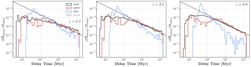
Figure 5: The delay time distribution of BBHs, BHNSs, and BNSs for the model with $\alpha_{\rm{CE}}=2.0$ and $\beta=0.5$. The left, middle, and right panels are the delay times for binaries formed at $z=0.2,2.0,$ and $6.0$, respectively.

4 Discussion

One of our key findings is that uncertainties in massive binary stellar evolution have a relatively small impact on the merger rate slopes, but can have a significant impact on the local merger rate and overall number of mergers. Specifically, the slopes of the merger rate are typically within a factor of $\lesssim 3\times$ in a given redshift range while the intrinsic rates span factors up to $\sim 1000\times$. These findings are in agreement with earlier work. For example, Belczynski et al. (2016) simulate the BBH merger rate for four different $\sigma_{\rm{rms}}^{\rm{1D}}$ models and find similar merger rate slopes between models but order of magnitude different merger rate normalizations. They also find higher $\sigma_{\rm{rms}}^{\rm{1D}}$ leading to fewer mergers, in agreement with our results in Figure 2. Riley et al. (2021) find that wind loss during the Wolf-Rayet phase does not significantly impact the BBH merger rate shape, Santoliquido et al. (2022) find similar shapes for the merger rate as a function of redshift when varying the common-envelope efficiency, mass transfer efficiency, and natal kicks, and Chu et al. (2022) find similar BNS merger rate slopes when varying the common envelope efficiency, $\sigma_{\rm{rms}}^{\rm{1D}}$, and supernova ejecta, with the exception of one model which only creates BNSs with long ($\gtrsim 1\,\rm{Gyr}$) delay times. A full review of the different merger rates predicted by different simulations is out of scope for this paper, but will be important to advance the field.

On the other hand, our study and these works do not explore many other key uncertainties including stellar evolution tracks (e.g., Agrawal et al., 2023; Romagnolo et al., 2023), alternative metallicity-dependent star formation rate models (e.g., Neijssel et al., 2019; Briel et al., 2022; Santoliquido et al., 2022; Chruślińska, 2022), and different initial stellar property distributions (e.g., Klencki et al., 2018; Chruślińska et al., 2020). The rapid increase in gravitational wave observations at increasing distances will improve measurements of the redshift evolution of the compact object merger rate (e.g., Abbott et al., 2021; Nitz et al., 2023; Godfrey et al., 2023; Callister & Farr, 2023; Payne & Thrane, 2023; Ray et al., 2023). Future studies should therefore further investigate how compact object mergers are impacted by the uncertainties omitted in this study. If the shape of the isolated binary merger rate is, however, robust across uncertainties in massive binary star evolution, it would support the potential for using the observed merger rate in tandem with simulations to constrain other uncertainties such as the star formation history and formation channel contributions.

5 Conclusion

In this study, we presented the expected cosmological merger rates of BBHs, BHNSs, and BNSs for the isolated binary channel using population synthesis simulations generated with COMPAS. We used two two-dimensional grids of models for binary evolution to investigate the impact of stellar evolution uncertainties. To analyze and quantify the redshift evolution of the merger rate in our simulations, we parameterized the merger rate using the rate at $z\sim 0$, the redshift of the peak merger rate ($z_{\rm peak}$), and the differentials for several redshift intervals as a proxy for the slopes (Equation 3). We summarize our main findings below:

1. The redshift evolution of the BBH, BHNS, and BNS merger rates follow a remarkably similar shape for all our simulations (Figure 2): they increase from $z\sim 0$ until a peak between $z=1.2$–$2.4$, and then decline until our assumed beginning of star formation at $z=10$. Although the local ($z\sim 0$) merger rate and overall normalization vary by factors up to $1000\times$ between models, the slopes (quantified with the differential from Equation 3) typically vary with factors of $1$–$3\times$ (Figure 3).

2. The shape of the merger rate across redshift is correlated with specific binary evolution parameters (Figure 4). Future observations of mergers to high redshifts can therefore help constrain models for binary evolution.

3. We find that the common-envelope efficiency $\alpha_{\rm{CE}}$ dominates the redshift distribution of mergers in our grid A simulations (Figure 2). It has a non-monotonic impact on the merger rate, which is a result of a “‘sweet spot” range in which binaries both can successfully eject their CEs and are tightened enough to merge in a Hubble time.

4. The SN natal kick velocity dispersion $\sigma_{\rm{rms}}^{\rm{1D}}$ typically dominates the shape of the merger rate in our grid B simulations because strong kicks disrupt the binaries leading to a drastic decrease in the efficiency of DCO formation (Figure 2, Figure 6).

Appendix A Simulation Settings

Table 2 provides a summary of our assumptions for the COMPAS population synthesis simulations.

Table 2: Initial values and default settings chosen for the population synthesis simulations performed with COMPAS in this study. Cyan and orange stars indicate prescriptions and assumptions that we vary in tandem (see Table 1).

Description and name	Value/range	Note / setting
Initial conditions
Initial mass $m_{1,\rm{i}}$	$[5,150]$$\,\rm{M}_{\odot}$	Kroupa (2001) IMF $\propto{m_{1,\rm{i}}}^{-\alpha}$ with $\alpha_{\rm{IMF}}=2.3$ for stars above $5$$\,\rm{M}_{\odot}$
Initial mass ratio $q_{\rm{i}}=m_{2,\rm{i}}/m_{1,\rm{i}}$	$[0,1]$	We assume a flat mass ratio distribution $p(q_{\rm{i}})\propto 1$ with $m_{2,\rm{i}}$ $\geq 0.1\,\rm{M}_{\odot}$
Initial semi-major axis $a_{\rm{i}}$	$[0.01,1000]$$\,\mathrm{AU}$	Distributed flat-in-log $p(a_{\rm{i}})\propto 1/{a_{\rm{i}}}$
Initial metallicity $Z_{\rm{i}}$	$[0.0001,0.03]$	Distributed flat-in-log $p(Z_{\rm{i}})\propto 1/{Z_{\rm{i}}}$
Initial orbital eccentricity ${e}_{\rm{i}}$	0	All binaries are assumed to be circular at birth
Fiducial parameter settings:
Stellar winds for hydrogen rich stars	Belczynski et al. (2010)	Based on Vink et al. (2000, 2001), including LBV wind mass loss with $f_{\rm{LBV}}=1.5$
Stellar winds for hydrogen-poor helium stars	Belczynski et al. (2010)	Based on Hamann & Koesterke (1998) and Vink & de Koter 2005
Max transfer stability criteria	$\zeta$-prescription	Based on Vigna-Gómez et al. (2018) and references therein
$\star$  Mass transfer accretion rate	thermal timescale	Limited by thermal timescale for stars Vigna-Gómez et al. (2018); Vinciguerra et al. (2020)
	Eddington-limited	Accretion rate is Eddington-limit for compact objects
Non-conservative mass loss	isotropic re-emission	Massevitch & Yungelson (1975); Bhattacharya & van den Heuvel (1991); Soberman et al. (1997)
		Tauris & van den Heuvel (2006)
Case BB mass transfer stability	always stable	Based on Tauris et al. (2015, 2017), Vigna-Gómez et al. (2018)
CE prescription	$\alpha-\lambda$	Based on Webbink (1984); de Kool (1990)
$\star$  CE efficiency $\alpha$-parameter	0.5
CE $\lambda$-parameter	$\lambda_{\rm{Nanjing}}$	Based on Xu & Li (2010a, b) and Dominik et al. (2012)
Hertzsprung gap (HG) donor in CE	pessimistic	Defined in Dominik et al. (2012): HG donors don’t survive a CE phase
SN natal kick magnitude $v_{\rm{k}}$	$[0,\infty)$$\,\rm{km}\,\rm{s}^{-1}$	Drawn from Maxwellian distribution with standard deviation $\sigma_{\rm{rms}}^{\rm{1D}}$
SN natal kick polar angle ${\theta}_{\rm{k}}$	$[0,\pi]$	$p({\theta}_{\rm{k}})=\sin({\theta}_{\rm{k}})/2$
SN natal kick azimuthal angle $\phi_{k}$	$[0,2\pi]$	Uniform $p(\phi)=1/(2\pi)$
SN mean anomaly of the orbit	$[0,2\pi]$	Uniformly distributed
$\star$  Core-collapse SN remnant mass prescription	delayed	From Fryer et al. (2012), which has no lower BH mass gap
USSN remnant mass prescription	delayed	From Fryer et al. (2012)
ECSN remnant mass presciption	$m_{\rm{f}}=1.26\,\rm{M}_{\odot}$	Based on Equation 8 in Timmes et al. (1996)
$\star$  Core-collapse SN velocity dispersion $\sigma_{\rm{rms}}^{\rm{1D}}$	265$\,\rm{km}\,\rm{s}^{-1}$	1D rms value based on Hobbs et al. (2005)
USSN and ECSN velocity dispersion $\sigma_{\rm{rms}}^{\rm{1D}}$	30$\,\rm{km}\,\rm{s}^{-1}$	1D rms value based on e.g., Pfahl et al. (2002); Podsiadlowski et al. (2004)
PISN / PPISN remnant mass prescription	Marchant et al. (2019)	As implemented in Stevenson et al. (2019)
Maximum NS mass	$\rm{max}_{\rm{NS}}=2.5$$\,\rm{M}_{\odot}$	Following Fryer et al. (2012)
Tides and rotation		We do not include prescriptions for tides and/or rotation
Simulation settings
Sampling method	STROOPWAFEL	Adaptive importance sampling from Broekgaarden et al. (2019).
Binary fraction	$f_{\rm{bin}}=1$	Corrected factor to be consistent with e.g., Sana (2016)
Solar metallicity $\,\rm{Z}_{\odot}$	$\,\rm{Z}_{\odot}$ = 0.0142	based on Asplund et al. (2009)
Binary population synthesis code	COMPAS	Team COMPAS: Riley et al. (2022)

Appendix B Formation rates as a function of redshift

Figure 6 shows the formation rate (i.e. number of DCOs formed) as a function of redshift for all our simulations. It is clear that the formation rates peak at higher redshifts than the merger rates in Figure 2 because there are non-negligible delays between binary formation and merger. For many models the formation rate peaks at higher redshifts compared to the star formation rate peak, which is a result of boosted DCO formation efficiency at low metallicities (see Boesky et al. 2024 for more details).

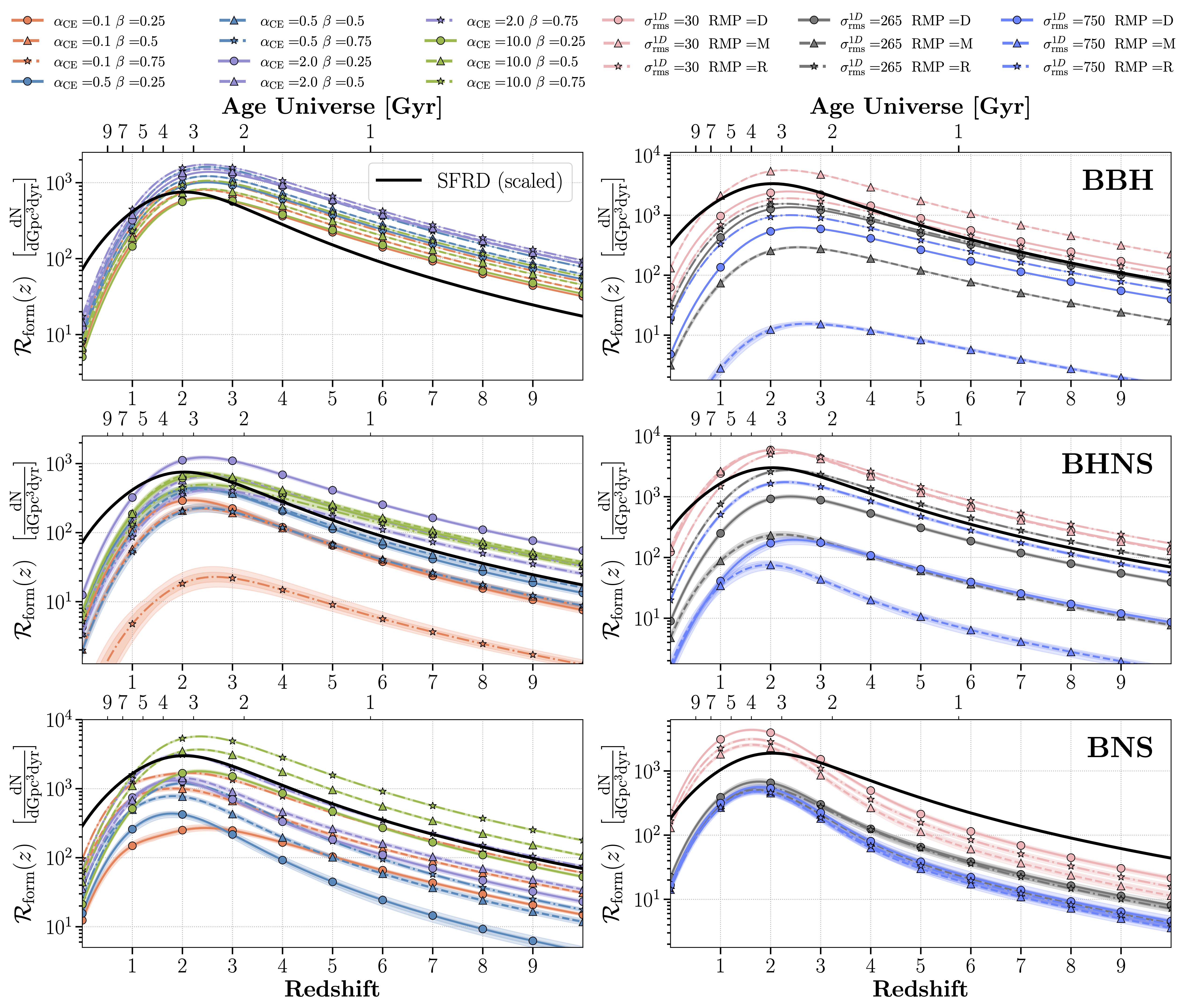
Figure 6: Same as Figure 2, but for the formation rates of BBH, BHNS, and BNS systems instead of merger rates. We define the formation time as directly after the second supernova when both compact objects have formed.

Appendix C Correlating Differentials With Binary Evolution Model Parameters

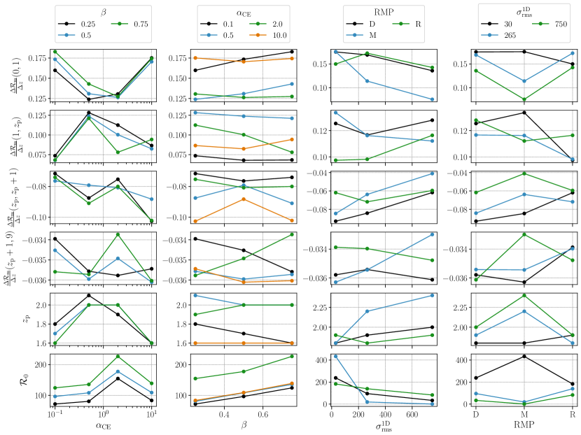
Figure 7: Differentials of the BBH merger rate in the redshift ranges $[0,1]$, $[1,z_{\rm{peak}}]$, $[z_{\rm{peak}},z_{\rm{peak}}+1]$, $[z_{\rm{peak}}+1,9]$ as well as $z_{\rm{peak}}$ and the local rate $\mathcal{R}_{0}$ plotted as a function of model parameters while keeping the second grid parameter fixed.

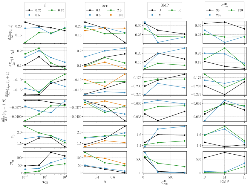
Figure 8: The same as Figure 7 but for BHNSs instead of BBHs.

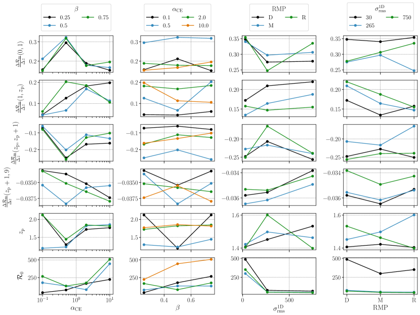
Figure 9: The same as Figure 7 but for BNSs instead of BBHs.

As detectors observe compact object mergers at increasing distances in the coming years, we will constrain the redshift evolution of the merger rate. Better constraints on the redshift evolution could enable us to tune population synthesis parameters by comparing the simulated and true redshift distribution of mergers. Parameterizing the merger rate redshift evolution with metrics such as the differential (Equation 3) will be important for quantifying and correlating features of $\mathcal{R}_{\rm{merge}}(z)$ with model parameters. To this end, we show the differential in several redshift ranges, $z_{\rm{peak}}$, and $\mathcal{R}_{0}$ as a function of model parameters for BBHs, BHNSs, and BNSs in Figure 7, Figure 8, and Figure 9, respectively. Besides how the BBH differentials correlate with $\alpha_{\rm{CE}}$ (described in Section 3), we leave the interpretation of trends in these figures to the reader.

References

- Aasi et al. (2015) Aasi, J., et al. 2015, Class. Quant. Grav., 32, 074001, doi: 10.1088/0264-9381/32/7/074001
- Abbott et al. (2021) Abbott, R., Abbott, T. D., Abraham, S., et al. 2021, The Astrophysical Journal Letters, 913, L7, doi: 10.3847/2041-8213/abe949
- Abbott et al. (2023) Abbott, R., Abbott, T. D., Acernese, F., et al. 2023, Physical Review X, 13, 041039, doi: 10.1103/PhysRevX.13.041039
- Acernese et al. (2015) Acernese, F., Agathos, M., Agatsuma, K., et al. 2015, Classical and Quantum Gravity, 32, 024001, doi: 10.1088/0264-9381/32/2/024001
- Adhikari et al. (2020) Adhikari, R. X., Arai, K., Brooks, A. F., et al. 2020, Classical and Quantum Gravity, 37, 165003, doi: 10.1088/1361-6382/ab9143
- Agrawal et al. (2023) Agrawal, P., Hurley, J., Stevenson, S., et al. 2023, Monthly Notices of the Royal Astronomical Society, 525, 933, doi: 10.1093/mnras/stad2334
- Akutsu et al. (2021) Akutsu, T., Ando, M., Arai, K., et al. 2021, Progress of Theoretical and Experimental Physics, 2021, 05A101, doi: 10.1093/ptep/ptaa125
- Asplund et al. (2009) Asplund, M., Grevesse, N., Sauval, A. J., & Scott, P. 2009, ARA&A, 47, 481, doi: 10.1146/annurev.astro.46.060407.145222
- Baibhav et al. (2019) Baibhav, V., Berti, E., Gerosa, D., et al. 2019, Phys. Rev. D, 100, 064060, doi: 10.1103/PhysRevD.100.064060
- Bavera et al. (2022) Bavera, S. S., Franciolini, G., Cusin, G., et al. 2022, A&A, 660, A26, doi: 10.1051/0004-6361/202142208
- Bavera et al. (2021) Bavera, S. S., Fragos, T., Zevin, M., et al. 2021, Astronomy & Astrophysics, 647, A153, doi: 10.1051/0004-6361/202039804
- Belczynski et al. (2010) Belczynski, K., Bulik, T., Fryer, C. L., et al. 2010, The Astrophysical Journal, 714, 1217, doi: 10.1088/0004-637x/714/2/1217
- Belczynski et al. (2010) Belczynski, K., Dominik, M., Bulik, T., et al. 2010, ApJ, 715, L138, doi: 10.1088/2041-8205/715/2/L138
- Belczynski et al. (2016) Belczynski, K., Holz, D. E., Bulik, T., & O’Shaughnessy, R. 2016, Nature, 534, 512, doi: 10.1038/nature18322
- Bhattacharya & van den Heuvel (1991) Bhattacharya, D., & van den Heuvel, E. P. J. 1991, Phys. Rep., 203, 1, doi: 10.1016/0370-1573(91)90064-S
- Boesky et al. (2024) Boesky, A., Broekgaarden, F. S., & Berger, E. 2024, doi: TBD
- Borhanian & Sathyaprakash (2022) Borhanian, S., & Sathyaprakash, B. S. 2022, arXiv e-prints, arXiv:2202.11048, doi: 10.48550/arXiv.2202.11048
- Briel et al. (2022) Briel, M. M., Eldridge, J. J., Stanway, E. R., Stevance, H. F., & Chrimes, A. A. 2022, MNRAS, 514, 1315, doi: 10.1093/mnras/stac1100
- Broekgaarden et al. (2019) Broekgaarden, F. S., Justham, S., de Mink, S. E., et al. 2019, MNRAS, 490, 5228, doi: 10.1093/mnras/stz2558
- Broekgaarden et al. (2021) Broekgaarden, F. S., Berger, E., Neijssel, C. J., et al. 2021, Monthly Notices of the Royal Astronomical Society, 508, 5028, doi: 10.1093/mnras/stab2716
- Broekgaarden et al. (2022) Broekgaarden, F. S., Berger, E., Stevenson, S., et al. 2022, Monthly Notices of the Royal Astronomical Society, doi: 10.1093/mnras/stac1677
- Callister & Farr (2023) Callister, T. A., & Farr, W. M. 2023, arXiv e-prints, arXiv:2302.07289, doi: 10.48550/arXiv.2302.07289
- Chruślińska et al. (2020) Chruślińska, M., Jeřábková, T., Nelemans, G., & Yan, Z. 2020, A&A, 636, A10, doi: 10.1051/0004-6361/202037688
- Chruślińska (2022) Chruślińska, M. 2022, Chemical evolution of the Universe and its consequences for gravitational-wave astrophysics, arXiv, doi: 10.48550/ARXIV.2206.10622
- Chu et al. (2022) Chu, Q., Yu, S., & Lu, Y. 2022, MNRAS, 509, 1557, doi: 10.1093/mnras/stab2882
- Collaboration et al. (2018) Collaboration, T. A., Price-Whelan, A. M., Sipőcz, B. M., et al. 2018, The Astronomical Journal, 156, 123, doi: 10.3847/1538-3881/aabc4f
- Collette (2013) Collette, A. 2013, Python and HDF5 (O’Reilly)
- de Kool (1990) de Kool, M. 1990, ApJ, 358, 189, doi: 10.1086/168974
- Dominik et al. (2012) Dominik, M., Belczynski, K., Fryer, C., et al. 2012, ApJ, 759, 52, doi: 10.1088/0004-637X/759/1/52
- Dorozsmai & Toonen (2024) Dorozsmai, A., & Toonen, S. 2024, MNRAS, doi: 10.1093/mnras/stae152
- Eggleton et al. (1989) Eggleton, P. P., Fitchett, M. J., & Tout, C. A. 1989, ApJ, 347, 998, doi: 10.1086/168190
- Evans et al. (2021) Evans, M., Adhikari, R. X., Afle, C., et al. 2021, arXiv e-prints, arXiv:2109.09882, doi: 10.48550/arXiv.2109.09882
- Fryer et al. (2012) Fryer, C. L., Belczynski, K., Wiktorowicz, G., et al. 2012, ApJ, 749, 91, doi: 10.1088/0004-637X/749/1/91
- Godfrey et al. (2023) Godfrey, J., Edelman, B., & Farr, B. 2023, arXiv e-prints, arXiv:2304.01288, doi: 10.48550/arXiv.2304.01288
- Gupta et al. (2023) Gupta, I., Afle, C., Arun, K. G., et al. 2023, arXiv e-prints, arXiv:2307.10421, doi: 10.48550/arXiv.2307.10421
- Hamann & Koesterke (1998) Hamann, W. R., & Koesterke, L. 1998, A&A, 335, 1003
- Harris et al. (2020) Harris, C. R., Millman, K. J., van der Walt, S. J., et al. 2020, Nature, 585, 357–362, doi: 10.1038/s41586-020-2649-2
- Hobbs et al. (2005) Hobbs, G., Lorimer, D. R., Lyne, A. G., & Kramer, M. 2005, MNRAS, 360, 974, doi: 10.1111/j.1365-2966.2005.09087.x
- Hopkins et al. (2014) Hopkins, P. F., Kereš, D., Oñorbe, J., et al. 2014, MNRAS, 445, 581, doi: 10.1093/mnras/stu1738
- Hunter (2007) Hunter, J. D. 2007, Computing in Science and Engineering, 9, 90, doi: 10.1109/MCSE.2007.55
- Hurley et al. (2000) Hurley, J. R., Pols, O. R., & Tout, C. A. 2000, MNRAS, 315, 543, doi: 10.1046/j.1365-8711.2000.03426.x
- Hurley et al. (2002) Hurley, J. R., Tout, C. A., & Pols, O. R. 2002, MNRAS, 329, 897, doi: 10.1046/j.1365-8711.2002.05038.x
- Iacovelli et al. (2022) Iacovelli, F., Mancarella, M., Foffa, S., & Maggiore, M. 2022, ApJ, 941, 208, doi: 10.3847/1538-4357/ac9cd4
- Klencki et al. (2018) Klencki, J., Moe, M., Gladysz, W., et al. 2018, Astronomy & Astrophysics, 619, A77, doi: 10.1051/0004-6361/201833025
- Kluyver et al. (2016) Kluyver, T., Ragan-Kelley, B., Pérez, F., et al. 2016, in ELPUB, 87–90
- Kroupa (2001) Kroupa, P. 2001, Monthly Notices of the Royal Astronomical Society, 322, 231, doi: 10.1046/j.1365-8711.2001.04022.x
- Ma et al. (2016) Ma, X., Hopkins, P. F., Faucher-Giguère, C.-A., et al. 2016, MNRAS, 456, 2140, doi: 10.1093/mnras/stv2659
- Madau & Dickinson (2014) Madau, P., & Dickinson, M. 2014, Annual Review of Astronomy and Astrophysics, 52, 415, doi: 10.1146/annurev-astro-081811-125615
- Madau & Fragos (2017) Madau, P., & Fragos, T. 2017, ApJ, 840, 39, doi: 10.3847/1538-4357/aa6af9
- Maggiore et al. (2020) Maggiore, M., Van Den Broeck, C., Bartolo, N., et al. 2020, J. Cosmology Astropart. Phys, 2020, 050, doi: 10.1088/1475-7516/2020/03/050
- Mandel & Broekgaarden (2022) Mandel, I., & Broekgaarden, F. S. 2022, Living Reviews in Relativity, 25, 1, doi: 10.1007/s41114-021-00034-3
- Mandel & Farmer (2022) Mandel, I., & Farmer, A. 2022, Phys. Rep., 955, 1, doi: 10.1016/j.physrep.2022.01.003
- Mandel & Müller (2020) Mandel, I., & Müller, B. 2020, Monthly Notices of the Royal Astronomical Society, 499, 3214, doi: 10.1093/mnras/staa3043
- Mapelli (2021) Mapelli, M. 2021, in Handbook of Gravitational Wave Astronomy, 16, doi: 10.1007/978-981-15-4702-7_16-1
- Marchant et al. (2019) Marchant, P., Renzo, M., Farmer, R., et al. 2019, ApJ, 882, 36, doi: 10.3847/1538-4357/ab3426
- Massevitch & Yungelson (1975) Massevitch, A., & Yungelson, L. 1975, Mem. Soc. Astron. Italiana, 46, 217
- Mehta et al. (2023) Mehta, A. K., Olsen, S., Wadekar, D., et al. 2023, New binary black hole mergers in the LIGO-Virgo O3b data. https://arxiv.org/abs/2311.06061
- Neijssel et al. (2019) Neijssel, C. J., Vigna-Gómez, A., Stevenson, S., et al. 2019, MNRAS, 490, 3740, doi: 10.1093/mnras/stz2840
- Ng et al. (2021) Ng, K. K. Y., Vitale, S., Farr, W. M., & Rodriguez, C. L. 2021, The Astrophysical Journal Letters, 913, L5, doi: 10.3847/2041-8213/abf8be
- Nitz et al. (2023) Nitz, A. H., Kumar, S., Wang, Y.-F., et al. 2023, ApJ, 946, 59, doi: 10.3847/1538-4357/aca591
- Olejak et al. (2022) Olejak, A., Fryer, C. L., Belczynski, K., & Baibhav, V. 2022, MNRAS, 516, 2252, doi: 10.1093/mnras/stac2359
- Olsen et al. (2022) Olsen, S., Venumadhav, T., Mushkin, J., et al. 2022, Phys. Rev. D, 106, 043009, doi: 10.1103/PhysRevD.106.043009
- Panter et al. (2004) Panter, B., Heavens, A. F., & Jimenez, R. 2004, MNRAS, 355, 764, doi: 10.1111/j.1365-2966.2004.08355.x
- Payne & Thrane (2023) Payne, E., & Thrane, E. 2023, Physical Review Research, 5, 023013, doi: 10.1103/PhysRevResearch.5.023013
- Perez & Granger (2007) Perez, F., & Granger, B. E. 2007, Computing in Science and Engineering, 9, 21, doi: 10.1109/MCSE.2007.53
- Pfahl et al. (2002) Pfahl, E., Rappaport, S., & Podsiadlowski, P. 2002, ApJ, 571, L37, doi: 10.1086/341197
- Podsiadlowski et al. (2004) Podsiadlowski, P., Langer, N., Poelarends, A. J. T., et al. 2004, ApJ, 612, 1044, doi: 10.1086/421713
- Pols et al. (1998) Pols, O. R., Schröder, K.-P., Hurley, J. R., Tout, C. A., & Eggleton, P. P. 1998, Monthly Notices of the Royal Astronomical Society, 298, 525, doi: 10.1046/j.1365-8711.1998.01658.x
- Punturo et al. (2010) Punturo, M., Abernathy, M., Acernese, F., et al. 2010, Classical and Quantum Gravity, 27, 194002, doi: 10.1088/0264-9381/27/19/194002
- Ray et al. (2023) Ray, A., Hernandez, I. M., Mohite, S., Creighton, J., & Kapadia, S. 2023, ApJ, 957, 37, doi: 10.3847/1538-4357/acf452
- Reitze et al. (2019) Reitze, D., Adhikari, R. X., Ballmer, S., et al. 2019, in Bulletin of the American Astronomical Society, Vol. 51, 35, doi: 10.48550/arXiv.1907.04833
- Riley et al. (2021) Riley, J., Mandel, I., Marchant, P., et al. 2021, Monthly Notices of the Royal Astronomical Society, 505, 663, doi: 10.1093/mnras/stab1291
- Romagnolo et al. (2023) Romagnolo, A., Belczynski, K., Klencki, J., et al. 2023, MNRAS, 525, 706, doi: 10.1093/mnras/stad2366
- Sana (2016) Sana, H. 2016, Proceedings of the International Astronomical Union, 12, 110–117, doi: 10.1017/S1743921317003209
- Santoliquido et al. (2022) Santoliquido, F., Mapelli, M., Artale, M. C., & Boco, L. 2022, Monthly Notices of the Royal Astronomical Society, 516, 3297, doi: 10.1093/mnras/stac2384
- Santoliquido et al. (2021) Santoliquido, F., Mapelli, M., Giacobbo, N., Bouffanais, Y., & Artale, M. C. 2021, Monthly Notices of the Royal Astronomical Society, 502, 4877, doi: 10.1093/mnras/stab280
- Sathyaprakash et al. (2012) Sathyaprakash, B., Abernathy, M., Acernese, F., et al. 2012, Classical and Quantum Gravity, 29, 124013, doi: 10.1088/0264-9381/29/12/124013
- Singh et al. (2022) Singh, N., Bulik, T., Belczynski, K., & Askar, A. 2022, Astronomy & Astrophysics, 667, A2, doi: 10.1051/0004-6361/202142856
- Soberman et al. (1997) Soberman, G. E., Phinney, E. S., & van den Heuvel, E. P. J. 1997, A&A, 327, 620. https://arxiv.org/abs/astro-ph/9703016
- Stevenson et al. (2019) Stevenson, S., Sampson, M., Powell, J., et al. 2019, ApJ, 882, 121, doi: 10.3847/1538-4357/ab3981
- Tauris et al. (2015) Tauris, T. M., Langer, N., & Podsiadlowski, P. 2015, MNRAS, 451, 2123, doi: 10.1093/mnras/stv990