SAUNAS I: Searching for Low Surface Brightness X-ray Emission with Chandra/ACIS

Abstract

We present SAUNAS (Selective Amplification of Ultra Noisy Astronomical Signal), a pipeline designed for detecting diffuse X-ray emission in the data obtained with the Advanced CCD Imaging Spectrometer (ACIS) of the Chandra X-ray Observatory. SAUNAS queries the available observations in the Chandra archive, performs photometric calibration, PSF (point spread function) modeling and deconvolution, point-source removal, adaptive smoothing, and background correction. This pipeline builds on existing and well-tested software including CIAO, vorbin, and LIRA. We characterize the performance of SAUNAS through several quality performance tests, and demonstrate the broad applications and capabilities of SAUNAS using two galaxies already known to show X-ray emitting structures. SAUNAS successfully detects the 30 kpc X-ray super-wind of NGC 3079 using Chandra/ACIS datasets, matching the spatial distribution detected with more sensitive XMM-Newton observations. The analysis performed by SAUNAS reveals an extended low surface brightness source in the field of UGC 5101 in the 0.3–1.0 keV and 1.0–2.0 keV bands. This source is potentially a background galaxy cluster or a hot gas plume associated with UGC 5101. SAUNAS demonstrates its ability to recover previously undetected structures in archival data, expanding exploration into the low surface brightness X-ray universe with Chandra/ACIS.

1 Introduction

The Advanced CCD Imaging Spectrometer on the Chandra X-ray Observatory (Weisskopf et al., 2000, hearafter Chandra/ACIS) provides an effective balance between angular resolution and sensitivity for the study of diffuse galactic hot gas emission, with its field of view (FOV) up to $16.9\times 16.9$ arcmin² and 0.492 arcsec of spatial resolution. Stacking multiple observations made over Chandra’s 25$+$ year mission is one of the keys to obtaining the deepest observations of the universe in X-ray. However, in most cases, the position of the target on the detector changes within observations, introducing serious challenges to acquiring a meaningful combined image. The PSF (point spread function) broadens and becomes more ellipse-shaped with increasing off-axis angle, necessitating an elaborate deconvolution scheme and hampering the ability to exploit the full capabilities of the archive. Consequently, Chandra observations are under-explored to date in studies advancing the low X-ray surface brightness (SB) domain.

Future studies of low X-ray SB emission ($\sim$$10^{-8}$ to $10^{-11}$ s^-1 cm^-2 arcsec^-2 and beyond) enabled by data processed to enhance detection of low-count regions could advance progress in several currently open questions relevant to galaxy evolution, including the origins of diffuse soft X-ray emission in galaxies and feedback involvement (Kelly et al., 2021; Henley et al., 2010).

Lambda Cold Dark Matter (LCDM) cosmology predicts filaments of diffuse gas from the cosmic web to accrete during their infall onto proto-galactic dark matter (DM) halos (White & Rees, 1978; White & Frenk, 1991; Benson & Devereux, 2010) where gas is heated to approximately the halo virial temperature ($T>10^{6}$ K). This plasma, further shaped by energy injection from active galactic nuclei (AGN, Diehl & Statler, 2008), supernovae (SN) and stellar winds (Hopkins et al., 2012), is detected as diffuse soft X-ray band emission around galaxies (Mulchaey, 2000; O’Sullivan et al., 2001; Sato et al., 2000; Aguerri et al., 2017). The origins and evolution of hot gas halos are important open questions in astrophysics, as halos are both the aftermath and active players of gas feedback processes, which modulate the star formation efficiency in galaxies (Rees & Ostriker, 1977; Silk, 1977; Binney, 1977; White & Rees, 1978; White & Frenk, 1991). The largely-unexplored realm of extreme diffuse gas emission, likely associated with large departures from equilibrium (Strickland et al., 2004), is likely to preserve a unique historical record of these events. Such emission is also likely to be disregarded in studies using standard pipelines that are not optimized for preservation of statistically significant but low SB detections.

This project is the first in a series that will study the hot gas halos around galaxies using X-ray observations from the Chandra X-ray observatory. The first step is to test the pipeline to reduce the Chandra/ACIS data products, named SAUNAS (Selective Amplification of Ultra Noisy Astronomical Signal). This paper describes the SAUNAS pipeline processing of data from the Chandra Data Archive and benchmarks it to previous works. In particular, we focus on the comparison of results between our analyses and those from other investigations for two well-detected X-ray sources characterized in the literature: NGC 3079 and UGC 5101. The latter has complex and extended X-ray emission, previously unexplored and only revealed by the current work.

This paper is organized as follows. The SAUNAS pipeline is described in Sec. 2. The selection of published results for SAUNAS performance comparison is discussed in Sec. 3.1. The benchmark analysis is presented in Secs. 3.2, and 3.3. The discussion and conclusions are presented in Secs. 4 and  5, respectively. We assume a concordance cosmology ($\Omega_{\mathrm{M}}=0.3$, $\Omega_{\mathrm{\Lambda}}=0.7,H_{0}=70$ km s^-1 Mpc^-1, see Spergel et al., 2007). All magnitudes are in the AB system (Oke, 1971) unless otherwise noted.

2 Methodology

2.1 Observational challenges

From an observational perspective, measuring diffuse X-ray halo properties in galaxies involves at least four technical challenges:

1. Detection: The outskirts of X-ray halos are extremely faint ($\lesssim 10^{-8}$ – $10^{-11}$ s^-1 cm^-2 arcsec^-2). Separating the faint emission associated with sources from that of the X-ray background (Anderson & Bregman, 2011) within such low count regimes is an extraordinarily challenging task. Statistical methods that assume a normal (Gaussian) distribution may not produce accurate results.

2. Deblending: AGNs and XRBs are typically unresolved point sources that may contribute to the same X-ray bands where the hot gas halos are expected to emit (from $\sim 0.3-0.5$ to $1.2-2$ keV). While in principle the detection of hot gas halos in nearby galaxies may not require very high spatial resolution observations or spectral capabilities, the separation of such emission from that of point sources does require them. High spatial resolution observations reduce systematic contamination in low surface brightness regimes.

3. Point spread function (PSF) contamination: The distribution of diffuse emission is easily confused with the scattered, extended emission of the unresolved bright cores that contaminate the outskirts of the target through the extended wings of the PSF of the detector (Sandin, 2014, 2015). Most studies do not correct for this type of scattering effect, although a few works, such as Anderson et al. (2013), have explored the combined stacked hot gas halo emission of 2165 galaxies observed with ROSAT (0.5–2.0 keV), convolving the combined surface brightness profiles by the PSF model to take into account the dispersion of light.

4. Reproducibility & Accessibility: The methodologies for calibration, detection, and characterization of X-ray emission have substantial differences between studies. Due to the Poissonian nature of the X-ray emission, most studies employ different types of adaptive smoothing in their analysis. These software methods tend to be custom-made and infrequently made publicly available. Likewise, the final data products (final science frames) are seldom offered to the community.

The SAUNAS methodology presented in the current paper attempts to address most of these points by 1) correcting the PSF in the images, 2) separating the emission of point sources from that of diffuse extended ones, and 3) providing a quantitative metric to determine if a detection is real or not. These two points implemented in SAUNAS are the major difference with other existing codes for detection of extended X-ray emission, such as vtpdetect (Ebeling & Wiedenmann, 1993) or EXSdetect (Liu et al., 2013), as they do not attempt to deconvolve the observations using dedicated PSF models or to separate diffuse emission from point sources.

2.2 SAUNAS pipeline

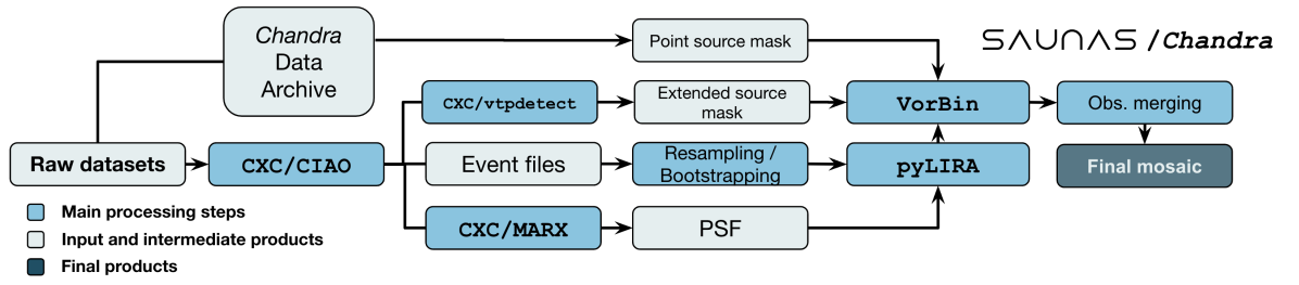
Figure 1: SAUNAS pipeline flowchart. From left to right: SAUNAS pre-calibrates the Chandra observations by first using Chandra X-ray Center (CXC)/CIAO, which generates the event files, extended source masks, and the PSFs. The events in each individual visit are first resampled via bootstrapping and then deconvolved using LIRA. Voronoi binning is applied to each deconvolved observation, and merged into a single flux map after sky background correction.

\begin{overpic}[trim=35.13124pt 20.075pt 35.13124pt 35.13124pt,clip,width=214.63977pt]{SAUNAS_CenA_5E6_ground_truth.png} \put(126.0,173.0){\color[rgb]{0,0,0} \hbox{\pagecolor{white}{Simulated source}}} \end{overpic}

\begin{overpic}[trim=35.13124pt 20.075pt 35.13124pt 35.13124pt,clip,width=214.63977pt]{SAUNAS_CenA_5E6_psf.png} \put(175.5,173.0){\color[rgb]{0,0,0} \hbox{\pagecolor{white}{PSF}}} \end{overpic}

\begin{overpic}[trim=35.13124pt 20.075pt 35.13124pt 35.13124pt,clip,width=214.63977pt]{SAUNAS_CenA_5E6_convolved.png} \put(107.0,173.0){\color[rgb]{0,0,0} \hbox{\pagecolor{white}{PSF convolved source}}} \end{overpic}

\begin{overpic}[trim=35.13124pt 20.075pt 35.13124pt 35.13124pt,clip,width=214.63977pt]{SAUNAS_CenA_5E6_events.png} \put(106.5,173.0){\color[rgb]{0,0,0} \hbox{\pagecolor{white}{Simulated observation}}} \end{overpic}

\begin{overpic}[trim=35.13124pt 0.0pt 35.13124pt 35.13124pt,clip,width=214.63977pt]{SAUNAS_CenA_5E6_LIRA.png} \put(122.5,188.0){\color[rgb]{0,0,0} \hbox{\pagecolor{white}{LIRA deconvolved}}} \end{overpic}

\begin{overpic}[trim=35.13124pt 0.0pt 35.13124pt 35.13124pt,clip,width=214.63977pt]{SAUNAS_CenA_5E6_voronoi.png} \put(103.0,188.0){\color[rgb]{0,0,0} \hbox{\pagecolor{white}{Final smoothed mosaic}}} \end{overpic}

Figure 2: SAUNAS analysis test on a synthetic dataset. Top left: Underlying distribution of the simulated test source. Top right: Point spread function (PSF) of the simulated observation. Central left: Simulated underlying distribution of the test source convolved by the PSF. Central right: Simulated observed events based on the PSF-convolved distribution. Bottom left: LIRA PSF deconvolved average posterior image. Bottom right: Adaptively smoothed final mosaic. Dashed contours represent the $3\sigma$ and dotted contours the $2\sigma$ detection level of X-ray emission. The equivalent exposure time for this test is $\tau_{\rm exp}=5\times 10^{6}$ s cm².

SAUNAS generates two main products: a) PSF-deconvolved X-ray adaptively smoothed surface brightness maps and b) signal-to-noise ratio (SNR) detection maps. The X-ray adaptively smoothed surface brightness maps provide the flux and luminosity of the hot gas X-ray halos, while the SNR detection maps provide the probability that the flux associated with each region on those maps is statistically higher than the local X-ray background noise.

SAUNAS creates these products in four major steps (see Fig. 1): 1) pre-processing of the archival Chandra X-ray observations using the Chandra Interactive Analysis of Observations software, (Fruscione et al., 2006, CIAO, hereafter, see Sec. 2.2.1), 2) statistical resampling of the X-ray detection events by bootstrapping, 3) PSF deconvolution of the event maps using the Bayesian Markov Chain Monte Carlo (MCMC) LIRA tool (Low-counts Image Reconstruction and Analysis, Donath et al. (2022b); see Sec. 2.2.3), and 4) adaptive smoothing using VorBin (see Sec. 2.2.4). SAUNAS requires a few user-input parameters, including the location of the target ($\alpha$, $\delta$), field-of-view (FOV), and energy band. The main steps of the pipeline are described in the following subsections.

2.2.1 CIAO pre-processing

First, the data is pre-processed using CIAO in the following way:

1. All available Chandra/ACIS observations containing the user-supplied sky coordinates are identified using find_chandra_obsid. The datasets and their best available calibration files are automatically downloaded using (download_chandra_obsid and download_obsid_caldb).

2. The raw observations are reprocessed using chandra_repro (v4.16). To avoid over-subtraction of both the source and background counts necessary for the statistical analysis, the particle background cleaning subprocess is set (check_vf_pha) to “no”. See the main CIAO manual for more information on this step.

3. All the available ACIS datasets are merged into a single events file (merge_obs). This product serves as the phase 1 (first pass) observation file and is used to identify emission regions and to determine the source spectra needed for PSF construction.

4. The phase 1 merged observation file is used to define the angular extent of detected emission sufficient for basic spectral characterization. The spectral information is used in the step following this one. The VorBin (Cappellari & Copin, 2003) library generates a map of Voronoi bins, from which and a surface brightness profile is constructed. The preliminary detection radius ($R_{\rm lim,0}$), defined as the radial limit having a surface brightness equal to $10\%$ of the surface brightness at the central coordinates, is computed. If $R_{\rm lim,0}$ is undefined due to a low central surface brightness, the presence of detectable emission is unlikely. For such cases, $R_{\rm lim,0}$ is arbitrarily set to 1/4 of the FOV defined by the user. The events inside this detection radius are used to construct a spectrum employed in the next step to define the deconvolution kernel (e.g., PSF) appropriate for this target. The choice of a $10\%$ limit is an optimal compromise based on the analysis of Chandra/ACIS observations: including as much emission as possible from the source enhances the spectra used to generate the PSF. However, including a region too large reduces computational efficiency. Note that the spectrum derived in this step serves the sole purpose of informing PSF construction and is not intended for physical characterization of the gas.

5. CIAO’s task simulate_psf, in combination with the spectral information provided by the previous step, is used to generate a PSF representative of each observing visit to the target. The PSF modeling is dependent on the spectra of both the source and the background region, as well as the target position within the detector (off-axis angle). The latter is unique to each visit. The preliminary detection radius defines both the circular ($R<R_{\rm lim,0}$) and annular ($R_{\rm lim,0}<R<2\,R_{\rm lim,0}$) apertures used to measure the source and background spectra, respectively (specextract). The aspectblur is set to 0.25, and the number of iterations to 1000 per dataset.

6. Finally, the individual event files and PSFs corresponding to each visit are cropped to a cutout, with the preferred energy range selected.

The outputs from the pre-processing procedure with CIAO  described above, are: 1) the detected event maps (named obsid_Elow-upper_flt_evt.fits, where low and upper refer to the energy range limits and obsid is the observation ID identification in the Chandra archive), 2) the exposure time maps (obsid_Elow-upper_flt_expmap.fits), 3) the flux maps (obsid_Elow-upper_flt_flux.fits), and 4) the PSF (obsid_Elow-upper_flt_psf.fits). This set of intermediate files is used in the remaining steps of the SAUNAS pipeline to generate the final maps.

2.2.2 X-ray event resampling: bootstrapping

The X-ray sky background is a very low count regime. Bartalucci et al. (2014) obtained a flux of $10.2^{+0.5}_{-0.4}\times 10^{-13}$ erg cm^-2 deg^-2 s^-1 for the 1–2 keV band and 3.8$\pm{0.2}\times 10^{-12}$ erg cm^-2 deg^-2 s^-1 for the 2–8 keV band. This flux is equivalent to $\sim$ 0.03–0.003 photons arcsec^-2 (1–2 keV) and $\sim$ 0.01–0.001 photons arcsec^-2 for a typical $t=10^{4}$–$10^{5}$ s exposure (She et al., 2017). As a consequence, the signal from spurious groups of a few counts can dominate the shape of the Voronoi bins used for adaptive smoothing in each simulation if appropriate statistical methods are not implemented.

To enhance the robustness of the adaptively smoothed mosaics and to reduce contamination from non-significant signal in the background, the X-ray events are re-sampled via replacement (bootstrapping) as an additional (and user-optional) step before deconvolution. Bootstrapping is especially well-suited for inferring the uncertainties associated with an estimand – such as the median surface brightness in cases for which the Gaussian standard deviation regime does not apply or parametric solutions are too complicated or otherwise unknown. Bootstrapping effectively reduces the leverage that single events or very low count sources may have in the background of the final mosaics by accounting for the photon-noise uncertainties in the PSF deconvolution and Voronoi binning steps through a non-parametric approach, allowing for a better assessment of the uncertainties in the final simulations.

In our application, bootstrapping generates $N$$\sim 100$ (hereafter, $N_{\rm{boot}}$) new X-ray event samples from the observed sample, preserving size (flux) and permitting events to be repeated. While the number of bootstrapping simulations is set to 100 by default as a compromise between precision and computational resources, $N_{\rm{boot}}$ can be defined by the user in SAUNAS. Each resampled list of events is translated into an image, which is fed into the next step, PSF deconvolution (Sec. 2.2.3).

2.2.3 LIRA PSF deconvolution

The LIRA (Connors et al., 2011; Donath et al., 2022b) package deconvolves the emission from sources in X-ray data. Through the use of LIRA, SAUNAS removes the contamination from active galactic nuclei (AGNs) and X-ray binary stars (XRBs) which can be significantly extended and easily confused with a diffuse halo if the PSF is not accurately corrected. LIRA uses a Bayesian framework to obtain the best-fit PSF convolved model to the observations, allowing the user to evaluate the probability that a detection is statistically significant. LIRA was designed to provide robust statistics in the low-count Poissonian regimes representative of faint extended halos, the primary science focus of our project.

As detailed in Sec. 2.2.1, the PSF models are generated specifically for each target, taking into account their location in the detector and their spectral energy distributions, on a per-visit basis. SAUNAS deconvolves data from individual visits, using these PSF models as input into LIRA. Discrete hard-band emission is produced primarily by point sources, including AGNs (Fabbiano et al., 1989; Fabbiano, 2019), young stellar objects, and mass transfer onto the compact stellar object within XRB pairs (Wang, 2012). Because these point sources contaminate the soft band emission, they are excised from the data. They are identified using the Chandra Source Catalog (Evans et al., 2010), and then removed from the event file by deleting events that lay within the cataloged positional uncertainty ellipse of the source.

The Python implementation of LIRA is used to deconvolve the X-ray event files, thus minimizing the effects of the off-axis dependency associated with Chandra’s PSF, such that data from different visits can be combined in a later stage. LIRA accepts five input arrays: a) counts (number of events), b) flux (in  s^-1 cm^-2 px^-1), c) exposure ( s cm²), d) PSF, e) a first approximation to the background (counts). The first four inputs are generated by the CIAO pipeline (Sec. 2.2.1), while the initial baseline background is set to one. The number of LIRA simulations is set to 1000 (n_iter_max), in addition to 100 initial burn-in simulations (num_burn_in). To speed up the process, SAUNAS splits the LIRA simulations in parallel processing blocks (defined by the number of bootstrapping simulations), to be combined after the deconvolution process has finished. While 1000 LIRA simulations are run on each of the N$\sim$100 bootstrapping-resampled images described in Section 2.2.2, only the last LIRA realizations (those produced after the deconvolution process has stabilized) for each resampled image are used (hereafter, $N_{\rm{stable}}$), which typically is equal to $\sim$100. To save computational resources, $N_{\rm{stable}}$ is adapted based on the number of bootstrapping simulations so that the deconvolved dataset consists of a maximum of $N=N_{\rm{boot}}~{}\times N_{\rm{stable}}=~{}1000$ deconvolved images (posterior samples).

2.2.4 Adaptive Voronoi smoothing

The deconvolved datacubes, hereafter referred to as ”Bootstrapping-LIRA” realizations, serve as a proxy of the probability density distribution of the true X-ray emission on a pixel-per-pixel basis, at the Chandra/ACIS spatial resolution (a minimum of 0.492” px^-1, depending on the binning set by the user). To facilitate the detection of extended, low surface brightness structures such as hot gas halos – with apparent sizes substantially larger than the spatial resolution limit for the galaxies – the use of spatial binning enhances the detection of regions with very low signal-to-noise ratio.

Voronoi binning (VorBin, Cappellari & Copin, 2003) is applied to each of the $N$ posterior samples in the deconvolved datacube. This process generates $N$ Voronoi tesselation maps, each one differing from the other because they were calculated from the Bootstrapping-LIRA realizations. This dataset is a Voronoi map datacube representing the probability density distribution of the surface brightness of the target.

A consequence of this binning approach is the loss of spatial resolution in the faintest regions of the image (halos, background) compared to the brightest regions (i.e., the galactic cores). This loss is caused by the fact that the Voronoi technique varies the bin size in order to achieve a fixed signal-to-noise ratio in the resulting map. As we are primarily interested in mapping the large scale halo structures, this loss in spatial resolution does not significantly impact our science goals.

A surface brightness map is created by calculating the median across one of the axes of the Voronoi datacube. To prevent background emission from contaminating the final image, the scalar background level is determined individually for each realization of the Bootstrapping-LIRA datacube. All sources, both resolved and unresolved, must be meticulously masked prior to measuring the background level, to prevent systematically over-subtracting the background in the final mosaics. The source masking and background correction process are conducted iteratively:

1. After the LIRA deconvolution process and before the Voronoi binning is performed, point sources from the Chandra Source Catalog (CSC 2.0; likely X-ray binaries, SNe, AGNs) that lay in the image footprint are removed from the associated event file. Point source removal prevents the associated emission from impacting the adaptive Voronoi maps and resulting in diffuse contamination that could be confused with a gas halo component.

2. A secondary mask is generated using CIAO’s routine vtpdetect. This mask identifies the regions with detectable extended X-ray emission that are removed from the maps before measuring the background level. A mask is generated for each CCD of each visit through independent analysis. The masks are then combined into a single master extended source mask.

3. If a source was detected in the preliminary surface brightness profile generated a part of the CIAO pre-processing step (see Sec. 2.2.1, step 4), then those pixels with $R<R_{\rm lim,0}$ are also masked before the background assessment.

4. After removing all the masked pixels using the masks from the three previous steps, the first approximation of the background level ($B_{0}$) is made by measuring the median value of the unmasked sigma clipped ($\sigma=3$) pixels. The background value is then subtracted from the voronoi binned maps.

Once the individual observations have been background corrected, all the flux maps are combined using mean-weighting by the respective exposure times. Finally, a refined background value ($B_{1}$) is calculated using the combined observations by repeating the process described above. The noise level is then estimated from the background distribution as the ratio between the median background level and the lower limit of the $1\sigma$ error bar (equivalent to the $15.8\%$ percentile). The final background-subtracted, PSF-corrected, and Voronoi binned surface brightness maps are derived by using a median of the background-corrected bootstrapping-LIRA realizations. The final mosaics and the noise level are used to generate three different frames to be stored in the final products: 1) an average adaptive X-ray surface brightness map, 2) a noise level map, and 3) an SNR map.

2.3 Quality tests

\begin{overpic}[trim=80.29999pt 0.0pt 100.37498pt 40.15pt,clip,height=199.16928pt]{SAUNAS_test_diagnostic_model.png} \end{overpic}

Figure 3: Fraction of false positives and false negatives in the SAUNAS detection maps derived from two truth models as a function of the equivalent exposure time (cm² s). Blue symbols and lines represent the fraction of false negatives, while red represents the fraction of false positive detections in the mock maps. Cross symbols correspond to the double jet model and filled circles represent the cavity model (see Table 1). Vertical dashed lines indicate the median equivalent exposure times for the analyzed real observations in their respective bands.

This section presents the results from a series of quality tests designed to evaluate specific aspects of the output mosaics generated with SAUNAS:

1. Identify the fraction of false positives and false negative detections (Sec. 2.3.1).

2. Estimate the flux conservation of the deconvolution / Voronoi binning process (Sec. 2.3.2)

3. Quantify the quality of SAUNAS performance as compared to that of other methods (arestore, Sec. 2.3.3).

2.3.1 False positive / False negative ratio

For quality assessment, SAUNAS is tested using two different models varying the exposure time to reduce the photon flux and the detectability conditions:

1. A model of an idealized edge-on galaxy with two lobes emerging from a jet (double jet model).

2. A shell-like structure with a central bright source (cavity model).

The models are created as combinations of Gaussian 2D probability distributions (astropy.convolution.Gaussian2DKernel) with different ellipticities and rotations as described in Table 1. Following PSF convolution, a synthetic observed events map is generated using a random Poisson distribution (numpy.random.poisson).

The double jet model includes the emission from three sources: the galactic disk, a bright core, and the lobes. The range of surface brightnesses is $\sim$ 10^-6–10^-8 s^-1 cm^-2 arcsec^-2, excluding the considerably brighter (three to five orders of magnitude brighter) peak surface brightness of the core. Its morphology mimics the predominant structure observed in double jet radio galaxies such as Centaurus A (Hardcastle et al., 2007).

The other test simulation, a cavity model, contains a hollow shell with a central bright source. This model provides an important pipeline test for the reconstruction of cavities found in the intergalactic medium. The detection of cavity rims seen in projection against the diffuse emission from the hot intracluster and/or intergalactic medium is challenging. These large bubbles potentially provide a useful record of interactions between AGNs and the intergalactic medium, in which the expansion of the associated radio lobes excavate the surrounding medium (Pandge et al., 2021). Our test model is designed to be particularly challenging: an X-ray cavity with a dominant central source representing an AGN (Blanton et al., 2001; Dunn et al., 2010). The surface brightness background level of both models is fixed at $5\times 10^{-9}$ s^-1 cm^-2 arcsec^-2, and the equivalent exposure time is assumed to be flat an varying from $\tau_{\rm exp}=10^{8}$ to $\tau_{\rm exp}=10^{4}$ s cm². For reference, $\tau_{\rm exp}=5\times 10^{5}$ s cm², equals $\sim$10 ks at $0.3-1.0$ keV band.

Table 1: Photometric and structural properties of the synthetic test models. Columns: 1) Name, 2) Component, 3) Size, 4) Surface brightness, 5) Eccentricity, 6) Position angle.

Mock model	Component	Size	$\mu$	$q$	PA
(1)	(2)	(3)	(4)	(5)	(6)
		($\sigma_{x},\sigma_{y}$, pixels)	[s-1 cm-2 arcsec-2]		[∘]
Double jet	Core	1,1	1.2$\times$10-4	1	0
	Disk	15,3	$\sim$ 10-6–10-8	0.2	135
	Lobes	7,7	$\sim$ 10-6–10-8	1	0
	Jet	25,2	5$\times$10-7	0.08	45
	Background	–	5$\times$10-9	–	–
Cavity	Core	1,1	1.2$\times$10-4	1	0
	Shell	[30–45]	$\sim$ 10-7	1	0
	Background	–	5$\times$10-9	–	–

The synthetic data are generated using the real PSF associated with the Chandra/ACIS datasets of NGC 3656 (Arp 155, PID:10610775, Fabiano, G., Smith et al., 2012). This PSF, which displays the characteristic ellipsoid pattern of off-axis ACIS observations, is selected as a worst-case scenario, given its extreme ellipticity due to its off-axis position in the detector array. The readout streak is visible as a spike departing from the center of the PSF at a position angle of -70^∘ approximately (North $=0^{\circ}$, positive counter-clockwise).

The simulated observed events are passed to the SAUNAS pipeline for processing, followed by a comparison between the detected ($3\sigma$) maps and truth models. The quantitative quality test includes identification of the fraction of pixels that were incorrectly identified as false negatives (FN) and false positives (FP).

Fig. 2 demonstrates the deconvolution and smoothing process for a mock galaxy with $\tau_{\rm exp}=5\times 10^{6}$ s, having both diffuse X-ray emission and an extended PSF. The position angle selected for the model galaxy (Table 1) is selected specifically to offer a nontrivial test for the PSF deconvolution method. By using a position angle of $45^{\circ}$, the resulting convolved image displays two elongated features with apparently similar intensity (central left panel in Fig. 2, PSF convolved source): one real, and one created by the PSF. If the PSF elongated feature is removed in the final images, we can conclude that the image reconstruction was successful.

After Poisson sampling (see Simulated observation panel in Fig. 2), the resulting events map is equivalent to the processed CIAO event files. The events map shows broad emission for the core of the galaxy model in which the disk is indistinguishable. The two lobes are still present, but considerably blended with the emission from the inner regions. The events are then processed using SAUNAS (LIRA deconvolution, Bootstrapping, and vorbin steps).

The results from the PSF deconvolution (LIRA deconvolved panel in Fig. 2) show a removal of most of the PSF emission, recovering the signal from the disk of the galaxy and removing the PSF spike emission. However, a significant amount of noise is still visible, and the background level is difficult to estimate (lower left panel of Fig. 2).

After applying the bootstrapping and Voronoi binning methods, the resulting final corrected mosaic (final smoothed mosaic panel, Fig. 2) clearly shows the signal from the X-ray lobes, the disk, and the central bright core over the background. The $2\sigma$ and $3\sigma$ contours show the detected features following the calibration procedures described in Sec. 2, demonstrating complete removal of the PSF streak in the final mosaics (at a 99.7$\%$ of confidence level). The original shape and orientation of the disk is recovered, with the flux correctly deconvolved into the bright core of the model galaxy. Due to its dim brightness, the jet that connects the lobes with the main disk is notably distorted in the final mosaic, but still visible at a $2\sigma$ confidence level. For this test, the fraction of pixels unrecovered by the pipeline that were part of the model sources (false negatives, FN) is $FN=3.2\%$. On the other hand, the fraction of misidentified pixels that were part of the background (false positives, FP) is $FP=4.0\%$. The maps of false positives and false negatives for this test are available in Appendix B.

The test for the cavity model is repeated, sampling different equivalent exposure times. The results are shown in Appendix B. Fig. 3 presents a comparison of the false positive and false negative fraction as a function of the equivalent exposure time and model. For equivalent exposure times higher than $\tau_{\rm exp}=10^{6}$ s cm², the FP and FN are lower than 5–10%. These fractions increase towards shorter exposures as expected, showing a notable increase to 20$\%$ of false negatives (true source emission that is unrecovered by SAUNAS) at approximately $\tau_{\rm exp}=5\cdot 10^{5}$ s cm². The reason for this increase is the lack of detection of the dimmer outer regions in contrast with the brighter core (the lobes in the case of the double jet model, and the outer shell in the cavity model). Interestingly, the fraction of false positives does not increase substantially even at extremely low equivalent exposure times, remaining stable at $\sim 10\%$ down to $\tau_{\rm exp}<10^{4}$ s cm². This result demonstrates that even in cases of extremely short exposure times, SAUNAS is not expected to generate false positive detections, which is a critical requirement for our study.

2.3.2 Flux conservation

In an ideal scenario, the total flux of the events processed by SAUNAS should be equal to the total flux in the pre-processed frames by CIAO. In practice, the baseline model assumptions during the deconvolution process may affect the total flux in the resulting frames. LIRA assumes a flat background model that–combined with the counts in the source–tries to fit all the events in the image. However, deviations from this ideal scenario (non-uniform background, regions with different exposure time) generate differences between the input and output flux. In order to understand the impact of flux conservation in LIRA deconvolved images, we must 1) analyze the relative difference of flux before and after deconvolution, and 2) determine if the residuals of the deconvolution process generate any systematic artificial structure (i.e., photons may be preferentially lost around bright sources, generating holes in the image or erasing the dim signal from halos).

Total flux conservation is tested by measuring the ratio between the total flux in the input frames (those obtained at the end of the CIAO pre-processing, see Sec. 2.2.1) divided by the total flux in the final, SAUNAS processed frames. We perform this test on real (UGC 5101, see Sec. 3.3) and synthetic observations (Sec. 2.3.1). The results are shown in Fig. 4.

\begin{overpic}[trim=0.0pt 20.075pt 40.15pt 0.0pt]{flux_preservation_test.png} \end{overpic}

Figure 4: Flux conservation in SAUNAS frames. The histogram represents the probability distribution of the ratio between the recovered flux after SAUNAS processing and the total flux of the input, pre-processed frames.

A total flux loss of $\sim 5\%$ is detected in the SAUNAS processed frames when compared with the pre-processed event maps by CIAO. The results are consistent in real observations (recovered flux ratio of $95.0\pm 1.7$%) and in synthetic observations ($95.4^{+2.7}_{-2.4}$%). Using different simulations, we determined that this small flux loss is independent of the size of the FOV (in pixels), remaining stable at $\sim 5\%$. For the total area of the images analyzed, a 5% of lost flux is negligible and well within the stochastic uncertainty of typical photometry (see the error bars in the profiles described in Fig. 5). We consider a flux conservation ratio lower than 100% (i.e., 90% – 99%) as erring on the side of caution from a statistical perspective: the bias of LIRA to lose flux implies that SAUNAS will not generate false positive detections of hot gas halos.

2.3.3 Quality PSF deconvolution test

While Sec. 2.3.2 reported on the conservation of total flux in the image as a whole, this section discusses whether SAUNAS introduces unwanted artificial structures (fake halos, or oversubtracted regions) in the processed maps. For this test, two additional types of test sources are used: 1) a point source, and 2) a circular extended source. Both of these sources have been previously combined with a Chandra/ACIS PSF. To provide context, the results of LIRA are compared with those from CIAO/arestore.

The results are displayed in Fig. 10 (point source) and Fig. 11 (circular extended source) and detailed in Appendices A and B. To quantify the quality of the different deconvolution methods, radial surface brightness profiles of the truth (non convolved) model, the convolved simulated observations, and the resulting deconvolved maps are constructed. The profiles show that arestore tends to oversubtract the PSF, generating regions of negative flux around the simulated source. In the point source case scenario, arestore oversubtracts the background by more than $5\times 10^{-8}$ s^-1 cm^-2 px^-1, while LIRA recovers the background level with five times less residuals. The superiority of LIRA over arestore to recover diffuse structures is even more obvious in the extended source scenario (Fig. 11): arestore shows a clear oversubtraction ring-like region around the source, dipping the background level to $10^{-7.8}$ s^-1 cm^-2 px^-1 as compared to the real (truth model) level of $10^{-7}$ s^-1 cm^-2 px^-1. LIRA fits the background level significantly more faithfully, at a level of $\sim 10^{-7.2}$ s^-1 cm^-2 px^-1.

We conclude that LIRA deconvolution results are better suited for the detection of diffuse X-ray emission, such as extended hot gas halos, compared to other PSF correction techniques, such as CIAO’s arestore. Despite the model limitations described in Sec. 2.3.2, SAUNAS suppresses false positive extended emission detections without over-fitting the PSF, while recovering the true morphologies of X-ray hot gas distributions. Thanks to the modularity of SAUNAS, future updates in the LIRA deconvolution software will be automatically implemented in our pipeline, improving the quality of the processed frames.

3 Application to real observations

3.1 Sample selection

We identified two astrophysical targets of interest for testing the pipeline:

1. NGC 3079, a highly inclined barred spiral galaxy with a prominent Fermi bubble (Hodges-Kluck et al., 2020, the primary benchmarking target, see Sec. 3.2).

2. UGC 5101, an ultra-luminous IR galaxy that is undergoing a galactic merger (Sanders et al., 1988; Imanishi et al., 2001, the secondary benchmarking target, see Sec. 3.3).

The targets used to demonstrate SAUNAS capabilities were selected because they were known apriori to have extended soft X-ray emission detected by telescopes other than Chandra (NGC 3079), and the characterization of the extended emission was well-documented with a detailed methodology that could be replicated in the published research. Insisting that the data come from a different platform provides a truth model independent of systematic effects inherently associated with Chandra. Finally, these specific targets were selected in order to test SAUNAS against simple and complex emission structures associated with the different morphologies (a disk galaxy and an interacting system).

3.2 NGC 3079

\begin{overpic}[trim=0.0pt 0.0pt 0.0pt 0.0pt,clip,width=433.62pt]{NGC3079_filaments_composition.png} \put(10.0,440.0){\color[rgb]{0,0,0} \Large{{a)}}} \put(230.0,440.0){\color[rgb]{0,0,0} \Large{{b)}}} \put(230.0,220.0){\color[rgb]{0,0,0} \Large{{c)}}} \end{overpic}

Figure 5: Extended X-ray wind cones in NGC 3079, recovered in the Chandra/ACIS observations using SAUNAS. a) Broad-band (Chandra: 0.3–2.0 keV) surface brightness profiles of the four filaments identified by Hodges-Kluck et al. (2020) using XMM-Newton and GALEX observations. Top to bottom: All filaments, north-east, south-east, south-west, and north-west. Radial detection limits are in the panels (95% confidence level). b) SAUNAS processed image showing $2\sigma$ contours (black, shown in white in panel c)) with filament sectors in yellow. The radial detection limit indicated in panel a) for each of the four filaments is shown as solid yellow sectors, while that of “all filaments” is shown as dashed yellow, following the methodology found in Hodges-Kluck et al. (2020). The thick magenta circle in b) shows the maximum detection limit found with XMM-Newton, compatible with our results. c) Comparison of the optical morphology (Pan-STARRS $gri$) of NGC 3079 with the extended X-ray emission.

Large-scale bipolar winds, Fermi and radio bubbles, are examples of extended structures observed around the center of the Milky Way in multi-wavelength observations, including radio (MeerKAT, S-PASS), microwave (WMAP), mid-infrared (MSX), UV (XMM), X-rays (Chandra, XMM-Newton, ROSAT) and gamma rays (Fermi-LAT) (Sofue, 1995; Bland-Hawthorn & Cohen, 2003; Su et al., 2010; Finkbeiner, 2004; Carretti et al., 2013; Heywood et al., 2019). While the presence of these structures is well-known in our own galaxy, Li et al. (2019) reported the first non-thermal hard X-ray detection of a Fermi bubble in an external galaxy, NGC 3079 ($\alpha=150.491^{\circ}$, $\delta=+55.680^{\circ}$, $D=18.68\pm 1.32$ Mpc, 11.04 arcsec kpc^-1 Springob et al., 2005), using Chandra observations. Further works in X-ray and UV using XMM-Newton and GALEX revealed a 30 kpc long X-ray Galactic Wind Cone in NGC 3079 (up to 60 kpc in FUV, Hodges-Kluck et al., 2020), potentially associated with material that has been shocked by Type II supernovae.

The length of the X-ray wind cone of NGC 3079 ($R\sim 3$ arcmin, 16.3 kpc) contrasts with that of the bubble found by Li et al. (2019) using Chandra observations ($R\lesssim 0.75$ arcmin, 4.1 kpc). Hodges-Kluck et al. (2020) argued that the sensitivity of the longest Chandra observations in the soft X-ray band ($E<1$ keV) is affected by the molecular contaminant buildup on the detector window, and as a consequence, these Chandra/ACIS observations were only used for point source identification on NGC 3079 and subsequent masking for XMM-Newton.

Additionally, the available Chandra observations were much shallower (124.2 ks, with only 26.6 ks of usable exposure time due to contamination) than those of XMM (300.6 ks). Despite Fig. 6 in Hodges-Kluck et al. (2020) showing signs of faint extended emission in the Chandra/ACIS datasets, the authors did not attempt to characterize it. Because ancillary X-ray observations from XMM-Newton are available for this object, NGC 3079 is an ideal case for benchmarking the low surface brightness recovery capabilities of the SAUNAS pipeline.

To detect the X-ray galactic wind in NGC 3079, the same bandpass (0.3–2.0 keV) as in Hodges-Kluck et al. (2020) is used. The available Chandra/ACIS observations of NGC 3079 are detailed in Table 2. Each visit was reprocessed with independent PSF deconvolution, and then the visits were combined for Voronoi binning. Observations 19307 and 20947 were processed but discarded due to the presence of very large-scale gradients and unusually high background levels in the detectors where the main emission from NGC 3079 is located. After processing the remaining observations (2038 and 7851) with SAUNAS, extended emission observed by Chandra is compared to the results from XMM-Newton. The PSFs of the 2038 and 7851 observations and their unprocessed events are available in Figs.  16 and 18 in Appendices C and D respectively.

Following the results from Fig. 2 in Hodges-Kluck et al. (2020), four angular cone regions display diffuse emission: north-east ($\theta=40^{\circ}$), south-east ($\theta=110^{\circ}$), south-west ($\theta=-140^{\circ}$), and north-west ($\theta=-60^{\circ}$), ($\theta$ is measured counter-clockwise, north corresponds to $0^{\circ}$, see Fig. 5). Mimicking the methodology in the original article, an amplitude of $\pm 20^{\circ}$ is set for all the cones around their central axis. Surface brightness profiles are generated from the reprocessed Chandra observations, providing a direct comparison with previous results.

The results show that the extended X-ray wind emission is detectable using Chandra observations, up to a limit of $R_{\lim}\sim 40$ kpc from the center of NGC 3079 ($R_{\lim}=39.9^{+4.5}_{-5.1}$ kpc on average, extending up to $R_{\lim}=37.9^{+4.1}_{-4.4}$ kpc in the North-East filament) at a confidence level of 95% (2$\sigma$). The filament in the south-west of the galaxy is shortest at $R\sim$ 16–20 kpc. Interestingly, the XMM observations reveal a slightly larger extent in the X-ray emission on the west side (40 kpc) compared to the east side (30–35 kpc) according to Hodges-Kluck et al. (2020).. The average limiting surface brightness (95% confidence level) is $\mu=1.66^{+0.5}_{-0.5}\times 10^{-10}$ s^-1 cm^-2 arcsec^-2. Limiting surface brightness reaches its lowest limit when combining all the filaments, suggesting that the observations are limited by noise and not by systematic effects (if dominated by systematic gradients, a lower SNR would result from combining all the regions).

Table 2: Chandra/ACIS observations available within 10 arcmins of NGC 3079 and UGC 5101, retrieved from the Chandra Data Archive, as of February 2024 . Columns: 1) Observation ID, 2) Chandra instrument, 3) total exposure time per observation, 4) observation mode, 5) average count rate, 6) exposure start date.

Obs ID	Instrument	Exposure time	Mode	Count rate	Start date
(1)	(2)	(3)	(4)	(5)	(6)
		[$ks$]		[s-1]
NGC 3079
2038	ACIS-S	26.58	FAINT	10.27	2001-03-07
7851	ACIS-S	5.00	FAINT	14.88	2006-12-27
19307	ACIS-S	53.16	FAINT	6.14	2018-01-30
20947	ACIS-S	44.48	FAINT	6.10	2018-02-01
UGC 5101
2033	ACIS-S	49.32	FAINT	9.53	2001-05-31

3.3 UGC 5101

UGC 5101 ($z=0.039$, $D=161.8$ Mpc, 0.784 kpc arcsec^-1, Rothberg & Joseph, 2006) is an irregular galaxy that is undergoing a potential major merger. This object has previously been identified as a Seyfert 1.5 (Sanders et al., 1988), a LINER (low-ionization nuclear emission-line region) galaxy (Veilleux et al., 1995), and a Seyfert 2 galaxy (Yuan et al., 2010). UGC 5101 has a very extended optical tidal tail ($\sim 40$ kpc) to the west from the nucleus, with a second semicircular tidal tail that surrounds the bright core of the galaxy with a radius of 17 kpc (Surace et al., 2000). Radio, (Lonsdale et al., 2003), IR (Genzel et al., 1998; Soifer et al., 2000; Armus et al., 2007; Imanishi et al., 2001), and X-ray observations with Chandra and XMM-Newton (Ptak et al., 2003; González-Martín et al., 2009) suggest the presence of a heavily dust-obscured AGN in the nucleus of this galaxy.

The total exposure time and other information relevant to the Chandra/ACIS observations of UGC 5101 are provided in Table 2. The diffuse X-ray emission of UGC 5101 has been previously analyzed in the literature. Huo et al. (2004) found evidence for an inner hot gas halo of $8.7$ kpc (10.4″) and an outer halo of $14.3$ kpc (17.0″). Grimes et al. (2005) found that 95% of the 0.3–1.0 keV emission is enclosed in the inner 8.75 kpc galactocentric radius (10.5″). Smith et al. (2018, 2019) analyzed the Chandra/ACIS observations, finding that the 0.3–1.0 keV emission has a size of $24.0\arcsec\times 14.2\arcsec$ ($\sim 19.1\times 11.3$ kpc, position angle of 90^∘), and a total X-ray luminosity of $\log L_{X}=41.6$ erg s^-1.

\begin{overpic}[trim=20.075pt 25.09373pt 85.31874pt 38.14249pt,clip,height=199.16928pt]{UGC5101_soft_HST_Chandra_contours.png} \put(57.0,186.5){\color[rgb]{1,1,1}{{HST/ACS}}} \put(208.0,35.0){\color[rgb]{0,1,1}{{F435W}}} \put(167.0,25.0){\color[rgb]{0,1,0}{{F435W + F814W}}} \put(208.0,15.0){\color[rgb]{1,0,0}{{F814W}}} \end{overpic}\begin{overpic}[trim=70.2625pt 25.09373pt 10.03749pt 38.14249pt,clip,height=199.16928pt]{UGC5101_soft.png} \put(1.5,185.5){\color[rgb]{0,0,0} \hbox{\pagecolor{white}{Chandra/ACIS}}} \put(120.0,90.0){\color[rgb]{1,1,0}{{UGC\,5101}}} \put(20.0,150.0){\color[rgb]{1,1,0}{{X1}}} \put(136.0,13.0){\color[rgb]{0,0,0} \hbox{\pagecolor{white}{0.3-1.0 keV}}} \end{overpic}

\begin{overpic}[trim=20.075pt 25.09373pt 85.31874pt 38.14249pt,clip,height=199.16928pt]{UGC5101_medium_HST_Chandra_contours.png} \put(165.0,186.5){\color[rgb]{1,0,0}{{GMRT 150 MHz}}} \end{overpic}\begin{overpic}[trim=70.2625pt 25.09373pt 10.03749pt 38.14249pt,clip,height=199.16928pt]{UGC5101_medium.png} \put(1.5,185.5){\color[rgb]{0,0,0} \hbox{\pagecolor{white}{Chandra/ACIS}}} \put(136.0,13.0){\color[rgb]{0,0,0} \hbox{\pagecolor{white}{1.0-2.0 keV}}} \end{overpic}

\begin{overpic}[trim=20.075pt 0.0pt 85.31874pt 38.14249pt,clip,height=199.16928pt]{UGC5101_hard_HST_Chandra_contours.png} \end{overpic}\begin{overpic}[trim=70.2625pt 0.0pt 10.03749pt 38.14249pt,clip,height=199.16928pt]{UGC5101_hard.png} \put(1.5,185.5){\color[rgb]{0,0,0} \hbox{\pagecolor{white}{Chandra/ACIS}}} \put(121.5,27.8){\color[rgb]{0,0,0} \hbox{\pagecolor{white}{2.0-8.0 keV}}} \end{overpic}

Figure 6: Diffuse X-ray emission of UGC 5101 as detected with SAUNAS/Chandra in the 0.3–1.0 keV band (top), 1.0–2.0 keV band (central), and 2.0–8.0 keV band (bottom). Left: HST/ACS color image (red: F814W, green: F435W + F814W, blue: F435W). Upper Right: SAUNAS map of the diffuse X-ray emission, corrected for PSF effect, point-sources, and background. Solid contours represent $3\sigma$ detections and dotted contours the $2\sigma$ detection level of X-ray emission, represented in white (left panel) and black (right panel) for contrast. Solid red contours show GMRT 150 MHz data. White dashed ellipse represents the previous detection limits reported by Smith et al. (2019) of UGC 5101 in the same band.

Given these known robust detections, we employ SAUNAS in the characterization of the low surface brightness emission from UGC 5101. Three bandpasses are used, to ensure a direct comparison to the analyses by Smith et al. (2019): soft (0.3–1.0 keV), medium (1.0–2.0 keV), and hard (2.0–8.0 keV). The flux conservation ratio after PSF deconvolution in this exposure is $96.0\pm 0.02$% in the three bands. The processed X-ray emission maps are presented in Fig. 6, in comparison with the optical/NIR observations from HST, as well as ancillary radio observations for reference. The PSFs and unprocessed events of the UGC 5101 observations in the three bands analyzed are available in Figs. 17 and 19 in Appendices C and D, respectively.

The results are summarized in Fig. 6. The analysis of the Chandra/ACIS observations with SAUNAS reveal that even after PSF deconvolution, the soft X-ray emission of UGC 5101 still shows extended emission around its core. The 0.3–1.0 and 1.0–2.0 keV bands present X-ray emission with an elongated morphology, with a characteristic bright plume-like structure in the core, oriented in the north-south direction ($\mu_{\rm soft}$ = 1–2$\times$10^-8 s^-1 cm^-2 arcsec^-2), very similar to the results of Smith et al. (2018). In contrast, the hard band only shows a bright core in the center, compatible with an unresolved source. In the soft band, the diffuse X-ray emission is detectable down to levels of $\mu_{\rm soft}=$ 1.23${}^{+1.02}_{-0.66}$$\times 10^{-9}$ s^-1 cm^-2 arcsec^-2 ($2\sigma$), compared to the medium band level of $\mu_{\rm medium}=$ 1.25${}^{+1.38}_{-0.73}$$\times 10^{-9}$ s^-1 cm^-2 arcsec^-2 ($2\sigma$). Both soft and medium band emissions are centered over the main core of UGC 5101, showing the same orientation as observed by Smith et al. (2019). The soft band emission extends up to 25 arcsec (20 kpc) to the north and 17 arcsec (13.5 kpc) to the south ($3\sigma$).

The spatial distribution of X-ray emission around UGC 5101 is generally comparable to that detected in previous works (Smith et al., 2019). However, at approximately 40–60 arcsec radius to the north-east ($\alpha$, $\delta=143.980^{\circ}$, $+61.363^{\circ}$), the SAUNAS map reveals a diffuse bridge connecting with UGC 5101, at a $\sim 2\sigma$ level ($\mu_{\rm soft}\sim 6.2\times 10^{-10}$ s^-1 cm^-2 arcsec^-2 in the soft band). For clarity, we will refer to this extended emission as X1. Fig. 7 displays surface brightness profile analysis results and associated comparisons with X1. The central surface brightness of X1 is $\mu_{\rm soft}$ = 4.2${}^{+1.5}_{-1.3}\times 10^{-9}$ s^-1 cm^-2 arcsec^-2 in the soft band and $\mu_{\rm medium}$ = 1.54${}^{+0.76}_{-0.66}\times 10^{-9}$ s^-1 cm^-2 arcsec^-2 in the medium band. The emission of X1 is detectable at a $3\sigma$ confidence level with a comparable angular area to UGC 5101, but with a maximum surface brightness 20–30 times lower than the main object (see Fig. 7).

\begin{overpic}[trim=20.075pt 0.0pt 20.075pt 40.15pt,clip,height=199.16928pt]{UGC5101_profile_main} \end{overpic}

Figure 7: Surface brightness profiles of the diffuse X-ray emission of UGC 5101 and the extended diffuse north-east source (X1) detected with SAUNAS/Chandra in the 0.3–1.0 and 1.0–2.0 keV bands. Radially averaged surface brightness profile (blue upward triangles: 0.3–1.0 keV band, purple downward triangles: 1.0–2.0 keV band). Shaded areas represent the $1\sigma$ and $2\sigma$ error bars. Solid blue and dashed purple vertical lines represent the $2\sigma$ detection limits for the 0.3–1.0 keV and the 1.0–2.0 keV bands. Blue and purple stars show the average surface brightness of the north-east extended emission X1, represented at the measured galactocentric distance from UGC 5101.

Fig. 27 in Smith et al. (2019) shows a hint of what might be emission jutting to the North-East of UGC 5101 where we see X1, but at a considerably lower detectability. The X1 feature has not been discussed previously in the literature as part of the UGC 5101 system, but rather as a potential higher-$z$ galaxy cluster (Clerc et al., 2012; Koulouridis et al., 2021) in need of spectroscopic confirmation.

Observations of the Giant Metrewave Radio Telescope (GMRT) 150 MHz all-sky radio survey (Intema et al., 2017, see bottom left panel in Fig. 6) confirm the detection of an adjacent source centered over the recovered X-ray emission, with a surface brightness of $\mu=10^{-4}$ Jy arcsec^-2. The GMRT flux maps are shown as contours in Fig. 6, revealing a peak of radio emission over the center of X1 in addition to UGC 5101. GALEX UV observations provide a near-ultraviolet (NUV) flux of $5.14\pm 0.15\times 10^{-6}$ Jy (Seibert et al., 2012) but only upper limits in the far-ultraviolet (FUV) band ($9.8\cdot 10^{-6}$ Jy). Recent JWST observations (GO 1717, PI: Vivian U., MIRI) of UGC 5101 were inspected for this work, but they suffer from extreme saturation of the bright core of the galaxy, and the outer X-ray emitting region lies outside the footprint, so they were discarded for this study. While investigating the nature of this extended X-ray emission is beyond the scope of this paper focused on the presentation of the SAUNAS pipeline, we briefly discuss the main hypotheses (hot gas plume or high-$z$ galaxy cluster) in Sec. 4.

4 Discussion

4.1 Limitations

We have demonstrated the SAUNAS methodology to be successful in recovering dim, extended surface brightness X-ray features under low signal-to-noise ratio conditions through performance tests using both synthetic (Section 2.3) and real (Section 3) X-ray datasets.

There are, however, several limitations of SAUNAS in its current form that will be addressed in future versions of the pipeline. Among them, SAUNAS does not attempt to provide a quantitative separation between extended sources, such as a segmentation map. Deblending of extended X-ray sources is one of the main objectives of a complementary code, EXSdetect (Liu et al., 2013), using a friend-of-friends algorithm. Other specialized pipelines for X-ray observations, such as CADET, based on machine-learning algorithms, allow for the identification of specific source morphologies, such as X-ray cavities (Plšek et al., 2024). The potential combination of SAUNAS for generating low surface brightness detection maps with existing morphological identification and segmentation software will be explored in the future.

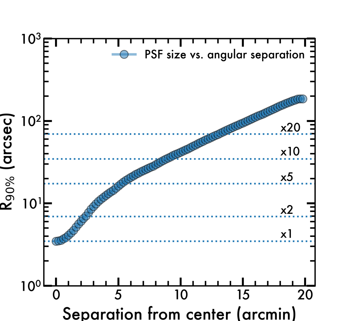
Figure 8: Variation of the Chandra/ACIS PSF size as a function of the angular separation to the center of the FOV. Vertical axis: Radius enclosing 90% of the flux from the PSF at 1.0 keV, based on the observations of UGC 5101. Horizontal axis: Angular separation to the center of the source, approximately the center optical axis. The horizontal dotted lines mark the PSF sizes that correspond to $\times 2$, $\times 5$, $\times 10$, and $\times 20$ the PSF size at its center ($\times 1$).

Another limitation of the SAUNAS pipeline is the precision of the PSF. The generation of the Chandra/ACIS PSFs depends on multiple factors, including, but not limited to, the position of the source on the detector, the SED of the source, or the specific parameters fed into the MARX simulation software (like the aspect blur). For example, LIRA deconvolution software only accepts one PSF for the whole image, and as a consequence, the shape of sources at high distances from the center of the image might be inaccurate. This phenomena can cause residuals if observations present bright sources at high angular distances from the center of the source, since the deconvolution will be based on the PSF at the center of the observation, but not at the location of the secondary contaminating source. As an attempt to quantify this effect, we estimate in Fig. 8 the variation of the PSF size ($R_{90\%}$, radius that contains 90% of the flux of a point source) vs.  angular separation to the source using CIAO psfsize_srcs, based on the Chandra/ACIS observations on UGC 5101. The results show that the PSF increases a factor of $\times$2 in $\sim$2 arcmin ($\times$10 in $\sim$10 arcmin). In our science cases, no bright object was observed in the environment of the main sources (NGC 3079, UGC 5101), so the main contributors to the scattered light are the sources for which the PSF was calculated. However, observers must be wary of strong residual PSF wings from nearby sources at $\sim$2 arcmin and longer distances. While a complete analysis of the uncertainties of the PSF in Chandra is out of the scope of the current paper, we refer to the Appendix in Ma et al. (2023) for a review in the field.

4.2 NGC 3079

The analysis of the Chandra/ACIS observations in the field of NGC 3079 revealed signs of X-ray wind out to galactocentric distances $R\sim 30$ kpc, compatible with previous observations using XMM–Newton (Hodges-Kluck et al., 2020). While XMM–Newton is able to trace the extended X-ray emission out to larger distances ($\sim$40 kpc) in some directions, some considerations must be made in order to compare XMM–Newton results with the benchmark study provided here:

1. XMM–Newton observations of NGC 3079 combine an $\sim$11 times longer exposure time (300.6 ks) than the usable time in Chandra/ACIS (26.6 ks) observations.

2. XMM-Newton has a larger effective area (4650 cm² at 1 keV) than Chandra ($555~{}$cm²), at the expense of a lower spatial resolution (XMM-Newton/FWHM $=$ 6 arcsec vs. Chandra/FWHM $=$ 0.2 arcsec). While the aperture is smaller, proper masking of point sources improves detectability of dim structures by reducing the background noise.

3. The analysis of the X-ray emission by Hodges-Kluck et al. (2020) is based on the inspection of the quadrant stacked images with a certain signal and radial threshold (see their Fig. 4, central panel). The methodology they use to calculate the limiting radius of the diffuse X-ray emission is not clearly stated in their analysis, making a direct and accurate comparison of results difficult.

Despite the differences of the detection methods, we conclude that SAUNAS is able to recover extended, low surface brightness X-ray emission using Chandra/ACIS X-ray observations of NGC 3079, in excellent agreement with the deeper exposure taken by XMM–Newton.

4.3 UGC 5101

Section 3.3 described evidence for extended low surface brightness emission (X1, $\mu_{\rm soft}$ = 4.2${}^{+1.5}_{-1.3}\times 10^{-9}$ s^-1 cm^-2 arcsec^-2, 0.3–1.0 keV) located in the north-east of the UGC 5101 merging galaxy. X1 has been previously detected in X-ray by Smith et al. (2019) but its emission was not discussed nor treated as part of UGC 5101’s outskirts. Other works (Clerc et al., 2012; Koulouridis et al., 2021) tentatively classified X1 as a potential background galaxy cluster, but this feature remained unconfirmed as spectroscopic observations are unavailable. X1 is detected also in GMRT 150 Mhz observations as a secondary source adjacent to UGC 5101, confirming the existence of a feature at this location. Two main hypotheses regarding the nature of X1 are:

1. X1 is part of the extended X-ray emitting envelope of UGC 5101.

2. X1 is a background source, potentially the extended envelope of a higher-$z$ object, such as a massive early-type galaxy or a cluster.

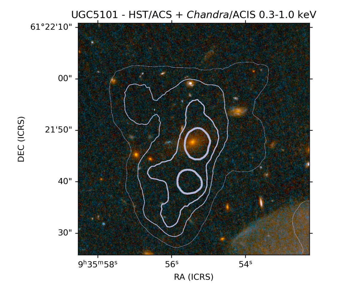
Figure 9: Hubble Space Telescope ACS imaging over the diffuse extended emission X1 found adjacent to UGC 5101. Pseudo-RGB color combination: Blue: F435W, Green: F435W $+$ F814W. Red: F814W. Grey contours represent the (3, 5, 7, and 10) $\sigma$ detection levels obtained in the 0.3–1.0 keV band from Chandra/ACIS observations, processed with SAUNAS. Notice the merger shell structure of UGC 5101 at the bottom right corner.

Although the X-ray emission in the soft and medium bands of X1 is adjacent to that of UGC 5101, and both objects have a dominant emission in the soft band compared to the medium and hard (see Figs.  6 and 7, the emission could still be part of a hot gas halo at higher-$z$. In fact, the center of the Chandra/ACIS X-ray emission overlaps remarkably well with that of a background galaxy. Fig. 9 shows the HST/ACS imaging (bands) centered over X1, with the soft-band X-ray emission contours overlapped for reference. The peak of X-ray emission is coincident with the position of a background galaxy (WISE J093555.43+612148.0). Unfortunately, WISE J093555.43+612148.0 does not have spectroscopic or photometric redshifts available.

While resolving the nature of X1 is beyond the scope of this paper, we conclude that the test performed with the Chandra/ACIS observations of UGC 5101 using SAUNAS demonstrates the pipeline’s capabilities in successfully producing adaptively smoothed, PSF-deconvolved X-ray images in different bands. The image reduction process presented here allows for a better calibration of the background to recover details at both high resolution and surface brightness (inner core structure of the merging galaxy) as well as extended ultra-low surface brightness regions, such as the previously unknown extended emission around UGC 5101.

5 Conclusions

In this paper we have presented SAUNAS: a pipeline to detect extended, low surface brightness structures on Chandra X-ray Observations. SAUNAS automatically queries the Chandra Archive, reduces the observations through the CIAO pipeline, generates PSF models and deconvolves the images, identifing and masking point sources, and generating adaptative smoothed surface brightness and detection SNR maps for the sources in the final mosaics. We have demonstrated through tests on simulated data and comparisons to published results that the SAUNAS pipeline distinguishes itself from other existing X-ray pipelines by meeting the following main objectives:

1. Generate X-ray detection maps for extended sources in a consistent, statistically reproducible way.

2. Provide a modular framework for reduction of Chandra/ACIS observations focusing on the detection of faint extended sources, simplifying the access to X-ray archival observations for multi-wavelength studies.

Our approach to meeting these objectives is to assess the statistical probability that signal in low-count areas is real. This strategy can both produce detections of previously-overlooked diffuse emission as well as minimize false positive detections of extended hot gas emission. In Sec. 3, we compare SAUNAS-processed archival Chandra/ACIS data to published results. This section demonstrates that the proposed methodology succeeds in recovering the extended emission detected in a selection of local Universe targets. While the CIAO pipeline provides a canonical and highly efficient procedure to reduce the Chandra observations, the secondary analysis of the resulting event files is usually performed in an independent way by the observers. Such a situation results in two suboptimal consequences: 1) Most X-ray studies are focused on single objects, or very small samples (three or four objects), and 2) most studies develop their own procedure to correct the PSF effects (if considered), to generate smoothed maps, and to determine the significance of emission over the background. Planned future work includes an analysis of the extended emission of nearby galaxies using Chandra/ACIS archival data, and releasing the tools to the astronomical community. In this first article, we made the processed maps available for the community through the Zenodo open repository.

A benefit of the automated functionality provided by this tool is its provision of straightforward access to high-level archival Chandra products and facilitation of their use in multi-wavelength studies. In future works of this series (Borlaff et al. in prep.) we will explore the X-ray emission of a sample of targets using the SAUNAS pipeline, focusing on the evolution of lenticular galaxies based on Chandra/ACIS data in combination with Hubble and Spitzer observations. The serendipitous discovery presented in this work in one of the galaxies studied; UGC 5101, an on-going merger galaxy, demonstrate that the combination of multi-wavelength legacy archives, such as those of Chandra, GMRT, and Hubble, may already hold the information to disentangle the impact of the different evolutionary drivers in galaxies.

Appendix A PSF deconvolution efficiency test

In this section, a set of synthetic observations generated with CIAO/MARX are used to evaluate the reliability of the SAUNAS algorithm when applied to a simple point source. SAUNAS’s ability to accurately recover diffuse emission is significantly governed by limitations imposed by LIRA, the associated deconvolution tool. SAUNAS could have instead utilized the widely-used and proven arestore tool, which can restore emission structures down to scales comparable to the Chandra/ACIS resolution (0.492″). Here we benchmark these two PSF deconvolution methodologies using simulated observations of an unresolved object constructed by convolving a point source with a highly off-axis PSF from Chandra/ACIS, associated with the observations of 3C 264 (NGC 3862, $\alpha=176.2709^{\circ}$, $\delta=+19.6063^{\circ}$, Obs. ID: 514). The simulated observations processed with SAUNAS (Sec. 2.2) are compared to the results produced by standard application of arestore. Both methods use the same number of iterations ($N_{\rm{iter}}=1000$). For each method, surface brightness profiles are constructed from Voronoi binning of the deconvolved data and compared to that of the model point source.

The results are shown in Fig. 10. The PSF convolved point source shows the characteristic elliptical shape of the off-axis PSF from Chandra/ACIS. The surface brightness profiles obtained from the images show that CIAO/arestore provides output images with more flux at their core than SAUNAS. However, CIAO/arestore’s deconvolved image has a higher noise in the surroundings of the center ($R=[0-10]$ px) than SAUNAS, including some clear signs of oversubtraction (see the Voronoi bins at the bottom right image) around the center of the object. In addition, CIAO/arestore leave a characteristic residual at larger distances ($R=[10-20]$ px) that could easily be confused with a shell of extended X-ray emission. In contrast, SAUNAS provides a deconvolved image with less central flux but a smoother transition to the background level and without the presence of residual halos of emission or oversubtraction. We conclude that CIAO/arestore concentrates more signal into a single point source at the expense of higher noise in the resulting images when compared to the methodology utilized by SAUNAS  described in Sec. 2.2.

Appendix B SAUNAS extended test models

Appendix A demonstrated that the combination of LIRA + Bootstrapping methods adopted in the SAUNAS pipeline provides a more accurate representation of the real distribution of light compared to CIAO/arestore, including avoiding arestore’s PSF over-subtraction. Given that the main aim of SAUNAS is the detection of extended sources, we extend the analysis from Appendix A to SAUNAS processing of an extended source model.

Figure 11 shows the result from this analysis. A simulated source with a central surface brightness of $\mu=$10^-3 s^-1 px^-1 and a background level of $\mu=$10^-7 s^-1 px^-1 is convolved with the same PSF used by the point source tests described in Appendix A. The resulting event file of convolved data is then processed by SAUNAS and deconvolved by a standard application of CIAO/arestore. A comparison of the associated surface brightness profiles provides both quantitative and qualitative assessments of the different light reconstruction methods.

The top right panel of Fig. 11 shows that the methodology adopted in SAUNAS produces a result that is more closely aligned with our science-driven requirements. Proper treatment of the fainter regions surrounding objects is a critical factor for the detection of faint extended emission, such as hot gas X-ray halos around galaxies. While SAUNAS produces a well-behaved profile that smoothly transitions to the background level at large radii, CIAO/arestore manufactures an over-subtracted background region surrounding the object, similar to its treatment of point sources (Appendix A).

Figures 12 and 13 show the results of the false positive / false negative quality test described in Sec. 2.3.1 for the double jet model. In Figs. 14 and 15 the equivalent results are shown for the cavity model. Each row represents different equivalent exposure times, from $\tau_{\rm exp}=5\times 10^{7}$ s cm²to $\tau_{\rm exp}=5\times 10^{4}$ s cm². We refer to the caption in the figures for details.

\begin{overpic}[trim=0.0pt 0.0pt 0.0pt 0.0pt,clip,width=212.47617pt]{ARESTORE_vs_LIRA_test_ID_Observed.png} \put(49.0,175.0){\color[rgb]{0,0,0} \hbox{\pagecolor{white}{PSF convolved point source}}} \end{overpic}

\begin{overpic}[trim=0.0pt 0.0pt 0.0pt 0.0pt,clip,width=212.47617pt]{ARESTORE_vs_LIRA_test_ID_profiles.png} \end{overpic}

\begin{overpic}[trim=0.0pt 0.0pt 0.0pt 0.0pt,clip,width=212.47617pt]{ARESTORE_vs_LIRA_test_ID_LIRA.png} \put(49.0,175.0){\color[rgb]{0,0,0} \hbox{\pagecolor{white}{SAUNAS}}} \end{overpic}

\begin{overpic}[trim=0.0pt 0.0pt 0.0pt 0.0pt,clip,width=212.47617pt]{ARESTORE_vs_LIRA_test_ID_arestore.png} \put(49.0,174.0){\color[rgb]{0,0,0} \hbox{\pagecolor{white}{CIAO/arestore}}} \end{overpic}

Figure 10: Point-source PSF deconvolution test. Top left panel: Emission from a point-source object and a background level of $\mu=$10^-7 s^-1 px^-1 convolved with a reference Chandra/ACIS PSF (NGC 3862, $\alpha=176.2709^{\circ}$, $\delta=+19.6063^{\circ}$, Obs. ID: 514). Top right panel: Surface brightness profiles of the convolved source (grey solid line), SAUNAS deconvolved image (blue dashed), and CIAO/arestore deconvolved (orange dotted) images. The horizontal dotted line represents the sky background of the model. Bottom left panel: SAUNAS deconvolved image. Bottom right panel: CIAO/arestore deconvolved image. Note that the convolved image (events map) and the CIAO/arestore deconvolved image have been processed using Voronoi binning for visualization purposes of the surface brightness. See the legend and colorbar in the figure.

\begin{overpic}[trim=0.0pt 0.0pt 0.0pt 0.0pt,clip,width=212.47617pt]{ARESTORE_vs_LIRA_test_ID_Observed_circle.png} \put(49.0,175.0){\color[rgb]{0,0,0} \hbox{\pagecolor{white}{PSF convolved circular source}}} \end{overpic}

\begin{overpic}[trim=0.0pt 0.0pt 0.0pt 0.0pt,clip,width=212.47617pt]{ARESTORE_vs_LIRA_test_ID_profiles_circle.png} \end{overpic}

\begin{overpic}[trim=0.0pt 0.0pt 0.0pt 0.0pt,clip,width=212.47617pt]{ARESTORE_vs_LIRA_test_ID_LIRA_circle.png} \put(49.0,175.0){\color[rgb]{0,0,0} \hbox{\pagecolor{white}{SAUNAS}}} \end{overpic}

\begin{overpic}[trim=0.0pt 0.0pt 0.0pt 0.0pt,clip,width=212.47617pt]{ARESTORE_vs_LIRA_test_ID_arestore_circle.png} \put(49.0,174.0){\color[rgb]{0,0,0} \hbox{\pagecolor{white}{CIAO/arestore}}} \end{overpic}

Figure 11: Extended source PSF deconvolution test. Top left panel: Emission from a circular source object with a central surface brightness of $\mu=$10^-3 s^-1 px^-1 and a background level of $\mu=$10^-7 s^-1 px^-1 convolved with a reference Chandra/ACIS PSF (NGC 3862, $\alpha=176.2709^{\circ}$, $\delta=+19.6063^{\circ}$, Obs. ID: 514). Top right panel: Surface brightness profiles of the ground-truth (non-PSF convolved) test source (red solid line), the PSF-convolved source (grey dashed-dotted line), SAUNAS deconvolved image (blue dashed), and CIAO/arestore deconvolved (orange dotted) images. The horizontal dotted line represents the sky background of the model, and the vertical dotted line represents the radial limit of the circular test source ($R=15$ pixels). Bottom left panel: SAUNAS deconvolved image. Bottom right panel: CIAO/arestore deconvolved image. Note that the convolved image (events map) and the CIAO/arestore deconvolved image have been processed using Voronoi binning for visualization purposes of the surface brightness. See the legend and colorbar in the figure.

\begin{overpic}[trim=25.09373pt 32.12pt 110.41249pt 30.11249pt,clip,height=108.405pt]{SAUNAS_CenA_1E7_events.png} \put(50.0,131.0){\color[rgb]{0,0,0} \hbox{\pagecolor{white}{$\tau_{\rm exp}=10^{7}$~{}s~{}cm${}^{2}$}}} \put(19.0,130.0){\color[rgb]{0,0,0} \hbox{\pagecolor{white}{Events}}} \end{overpic}

\begin{overpic}[trim=70.2625pt 32.12pt 110.41249pt 30.11249pt,clip,height=108.405pt]{SAUNAS_CenA_5E6_events.png} \put(50.0,131.0){\color[rgb]{0,0,0} \hbox{\pagecolor{white}{$\tau_{\rm exp}=5\times 10^{6}$~{}s~{}cm${}^{2}$}}} \end{overpic}

\begin{overpic}[trim=70.2625pt 32.12pt 25.09373pt 30.11249pt,clip,height=108.405pt]{SAUNAS_CenA_1E6_events.png} \put(50.0,131.0){\color[rgb]{0,0,0} \hbox{\pagecolor{white}{$\tau_{\rm exp}=10^{6}$~{}s~{}cm${}^{2}$}}} \end{overpic}

\begin{overpic}[trim=25.09373pt 32.12pt 110.41249pt 30.11249pt,clip,height=108.405pt]{SAUNAS_CenA_1E7_voronoi.png} \put(24.0,113.5){\color[rgb]{0,0,0} \hbox{\pagecolor{white}{Final}}} \end{overpic}

\begin{overpic}[trim=70.2625pt 32.12pt 110.41249pt 30.11249pt,clip,height=108.405pt]{SAUNAS_CenA_5E6_voronoi.png} \end{overpic}

\begin{overpic}[trim=70.2625pt 32.12pt 25.09373pt 30.11249pt,clip,height=108.405pt]{SAUNAS_CenA_1E6_voronoi.png} \end{overpic}

\begin{overpic}[trim=62.2325pt 0.0pt 80.29999pt 30.11249pt,clip,height=120.1096pt]{SAUNAS_CenA_1E7_FNFP.png} \put(19.0,127.0){\color[rgb]{0,0,0} \hbox{\pagecolor{white}{False positive/negative}}} \end{overpic}

\begin{overpic}[trim=102.38249pt 0.0pt 75.28125pt 30.11249pt,clip,height=120.1096pt]{SAUNAS_CenA_5E6_FNFP.png} \end{overpic}

\begin{overpic}[trim=100.37498pt 0.0pt 25.09373pt 30.11249pt,clip,height=120.1096pt]{SAUNAS_CenA_1E6_FNFP.png} \end{overpic}

Figure 12: SAUNAS processing test using the double jet model as a function of the equivalent exposure time (see Sec. 2.3.1 and Table 1). Top row shows the simulated event images. Middle row shows the final recovered surface brightness maps after processing with SAUNAS. Dashed contours represent the $3\sigma$ and dotted contours the $2\sigma$ detection level of X-ray emission. Bottom row represents the false positive (red) and false negative (blue) detection maps for each simulation (see Sec. 2.3.1). From left to right columns, the equivalent exposure times are $\tau_{\rm exp}=10^{7}$, $5\times 10^{6}$, and $10^{6}$ s cm². See the labels in the panels. Colorbars represent the number of events per pixel (event images) and the surface brightness flux (final mosaics).

\begin{overpic}[trim=25.09373pt 32.12pt 110.41249pt 30.11249pt,clip,height=108.405pt]{SAUNAS_CenA_5E5_events.png} \put(50.0,131.0){\color[rgb]{0,0,0} \hbox{\pagecolor{white}{$\tau_{\rm exp}=5\times 10^{5}$~{}s~{}cm${}^{2}$}}} \put(19.0,130.0){\color[rgb]{0,0,0} \hbox{\pagecolor{white}{Events}}} \end{overpic}

\begin{overpic}[trim=70.2625pt 32.12pt 110.41249pt 30.11249pt,clip,height=108.405pt]{SAUNAS_CenA_1E5_events.png} \put(50.0,131.0){\color[rgb]{0,0,0} \hbox{\pagecolor{white}{$\tau_{\rm exp}=10^{5}$~{}s cm${}^{2}$}}} \end{overpic}

\begin{overpic}[trim=70.2625pt 32.12pt 25.09373pt 30.11249pt,clip,height=108.405pt]{SAUNAS_CenA_5E4_events.png} \put(50.0,131.0){\color[rgb]{0,0,0} \hbox{\pagecolor{white}{$\tau_{\rm exp}=5\times 10^{4}$~{}s~{}cm${}^{2}$}}} \end{overpic}

\begin{overpic}[trim=25.09373pt 32.12pt 110.41249pt 30.11249pt,clip,height=108.405pt]{SAUNAS_CenA_5E5_voronoi.png} \put(24.0,113.5){\color[rgb]{0,0,0} \hbox{\pagecolor{white}{Final}}} \end{overpic}

\begin{overpic}[trim=70.2625pt 32.12pt 110.41249pt 30.11249pt,clip,height=108.405pt]{SAUNAS_CenA_1E5_voronoi.png} \end{overpic}

\begin{overpic}[trim=70.2625pt 32.12pt 25.09373pt 30.11249pt,clip,height=108.405pt]{SAUNAS_CenA_5E4_voronoi.png} \end{overpic}

\begin{overpic}[trim=62.2325pt 0.0pt 80.29999pt 30.11249pt,clip,height=120.1096pt]{SAUNAS_CenA_5E5_FNFP.png} \put(19.0,127.0){\color[rgb]{0,0,0} \hbox{\pagecolor{white}{False positive/negative}}} \end{overpic}

\begin{overpic}[trim=102.38249pt 0.0pt 75.28125pt 30.11249pt,clip,height=120.1096pt]{SAUNAS_CenA_1E5_FNFP.png} \end{overpic}

\begin{overpic}[trim=100.37498pt 0.0pt 25.09373pt 30.11249pt,clip,height=120.1096pt]{SAUNAS_CenA_5E4_FNFP.png} \end{overpic}

Figure 13: (Continuation of Fig. 12) SAUNAS processing test using the double jet model as a function of the equivalent exposure time (see Sec. 2.3.1 and Table 1). Top row shows the simulated event images. Middle row shows the final recovered surface brightness maps after processing with SAUNAS. Dashed contours represent the $3\sigma$ and dotted contours the $2\sigma$ detection level of X-ray emission. Bottom row represents the false positive (red) and false negative (blue) detection maps for each simulation (see Sec. 2.3.1). From left to right columns, the equivalent exposure times are $\tau_{\rm exp}=5\cdot 10^{5}$, $10^{5}$, and $5\times 10^{4}$ s cm². See the labels in the panels. Colorbars represent the number of events per pixel (event images) and the surface brightness flux (final mosaics).

\begin{overpic}[trim=25.09373pt 32.12pt 110.41249pt 30.11249pt,clip,height=108.405pt]{SAUNAS_Cave_1E7_events.png} \put(50.0,131.0){\color[rgb]{0,0,0} \hbox{\pagecolor{white}{$\tau_{\rm exp}=10^{7}$~{}s~{}cm${}^{2}$}}} \put(19.0,130.0){\color[rgb]{0,0,0} \hbox{\pagecolor{white}{Events}}} \end{overpic}

\begin{overpic}[trim=70.2625pt 32.12pt 110.41249pt 30.11249pt,clip,height=108.405pt]{SAUNAS_Cave_5E6_events.png} \put(50.0,131.0){\color[rgb]{0,0,0} \hbox{\pagecolor{white}{$\tau_{\rm exp}=5\times 10^{6}$~{}s~{}cm${}^{2}$}}} \end{overpic}

\begin{overpic}[trim=70.2625pt 32.12pt 25.09373pt 30.11249pt,clip,height=108.405pt]{SAUNAS_Cave_1E6_events.png} \put(50.0,131.0){\color[rgb]{0,0,0} \hbox{\pagecolor{white}{$\tau_{\rm exp}=10^{6}$~{}s~{}cm${}^{2}$}}} \end{overpic}

\begin{overpic}[trim=25.09373pt 32.12pt 110.41249pt 30.11249pt,clip,height=108.405pt]{SAUNAS_Cave_1E7_voronoi.png} \put(24.0,113.5){\color[rgb]{0,0,0} \hbox{\pagecolor{white}{Final}}} \end{overpic}

\begin{overpic}[trim=70.2625pt 32.12pt 110.41249pt 30.11249pt,clip,height=108.405pt]{SAUNAS_Cave_5E6_voronoi.png} \end{overpic}

\begin{overpic}[trim=70.2625pt 32.12pt 25.09373pt 30.11249pt,clip,height=108.405pt]{SAUNAS_Cave_1E6_voronoi.png} \end{overpic}

\begin{overpic}[trim=62.2325pt 0.0pt 80.29999pt 30.11249pt,clip,height=120.1096pt]{SAUNAS_Cave_1E7_FNFP.png} \put(19.0,127.0){\color[rgb]{0,0,0} \hbox{\pagecolor{white}{False positive/negative}}} \end{overpic}

\begin{overpic}[trim=102.38249pt 0.0pt 75.28125pt 30.11249pt,clip,height=120.1096pt]{SAUNAS_Cave_5E6_FNFP.png} \end{overpic}

\begin{overpic}[trim=100.37498pt 0.0pt 25.09373pt 30.11249pt,clip,height=120.1096pt]{SAUNAS_Cave_1E6_FNFP.png} \end{overpic}

Figure 14: SAUNAS processing test using the cavity model as a function of the equivalent exposure time (see Sec. 2.3.1 and Table 1). Top row shows the simulated event images. Middle row shows the final recovered surface brightness maps after processing with SAUNAS. Dashed contours represent the $3\sigma$ and dotted contours the $2\sigma$ detection level of X-ray emission. Bottom row represents the false positive (red) and false negative (blue) detection maps for each simulation (see Sec. 2.3.1). From left to right columns, the equivalent exposure times are $\tau_{\rm exp}=10^{7}$, $5\times 10^{6}$, and $10^{6}$ s cm². See the labels in the panels. Colorbars represent the number of events per pixel (event images) and the surface brightness flux (final mosaics).

\begin{overpic}[trim=25.09373pt 32.12pt 110.41249pt 30.11249pt,clip,height=108.405pt]{SAUNAS_Cave_5E5_events.png} \put(50.0,131.0){\color[rgb]{0,0,0} \hbox{\pagecolor{white}{$\tau_{\rm exp}=5\cdot 10^{5}$~{}s~{}cm${}^{2}$}}} \put(19.0,130.0){\color[rgb]{0,0,0} \hbox{\pagecolor{white}{Events}}} \end{overpic}

\begin{overpic}[trim=70.2625pt 32.12pt 110.41249pt 30.11249pt,clip,height=108.405pt]{SAUNAS_Cave_1E5_events.png} \put(50.0,131.0){\color[rgb]{0,0,0} \hbox{\pagecolor{white}{$\tau_{\rm exp}=10^{5}$~{}s~{}cm${}^{2}$}}} \end{overpic}

\begin{overpic}[trim=70.2625pt 32.12pt 25.09373pt 30.11249pt,clip,height=108.405pt]{SAUNAS_Cave_5E4_events.png} \put(50.0,131.0){\color[rgb]{0,0,0} \hbox{\pagecolor{white}{$\tau_{\rm exp}=5\cdot 10^{4}$~{}s~{}cm${}^{2}$}}} \end{overpic}

\begin{overpic}[trim=25.09373pt 32.12pt 110.41249pt 30.11249pt,clip,height=108.405pt]{SAUNAS_Cave_5E5_voronoi.png} \put(24.0,113.5){\color[rgb]{0,0,0} \hbox{\pagecolor{white}{Final}}} \end{overpic}

\begin{overpic}[trim=70.2625pt 32.12pt 110.41249pt 30.11249pt,clip,height=108.405pt]{SAUNAS_Cave_1E5_voronoi.png} \end{overpic}

\begin{overpic}[trim=70.2625pt 32.12pt 25.09373pt 30.11249pt,clip,height=108.405pt]{SAUNAS_Cave_5E4_voronoi.png} \end{overpic}

\begin{overpic}[trim=62.2325pt 0.0pt 80.29999pt 30.11249pt,clip,height=120.1096pt]{SAUNAS_Cave_5E5_FNFP.png} \put(19.0,127.0){\color[rgb]{0,0,0} \hbox{\pagecolor{white}{False positive/negative}}} \end{overpic}

\begin{overpic}[trim=102.38249pt 0.0pt 75.28125pt 30.11249pt,clip,height=120.1096pt]{SAUNAS_Cave_1E5_FNFP.png} \end{overpic}

\begin{overpic}[trim=100.37498pt 0.0pt 25.09373pt 30.11249pt,clip,height=120.1096pt]{SAUNAS_Cave_5E4_FNFP.png} \end{overpic}

Figure 15: (Continuation of Fig. 14) SAUNAS processing test using the double jet model as a function of the equivalent exposure time (see Sec. 2.3.1 and Table 1). Top row shows the simulated event images. Middle row shows the final recovered surface brightness maps after processing with SAUNAS. Dashed contours represent the $3\sigma$ and dotted contours the $2\sigma$ detection level of X-ray emission. Bottom row represents the false positive (red) and false negative (blue) detection maps for each simulation (see Sec. 2.3.1). From left to right columns, the equivalent exposure times are $\tau_{\rm exp}=5\times 10^{5}$, $10^{5}$, and $5\times 10^{4}$ s cm². See the labels in the panels. Colorbars represent the number of events per pixel (event images) and the surface brightness flux (final mosaics).

Appendix C NGC 3079 and UGC 5101 Point Spread Function

This section presents the PSFs generated for the NGC 3079 (see Sec. 3.2) and UGC 5101 (see Sec. 3.3), Chandra/ACIS observations. The PSFs were generated using MARX as described in Sec. 2.2. The panels in Figs. 16 and Fig. 17 show the different PSFs obtained for the three bands (0.3–1.0 keV, 1.0–2.0 kev, and 2.0–8.0 kev) in UGC 5101, and for the two datasets analyzed in the broadband (0.3–2.0 keV) for NGC 3079.

\begin{overpic}[trim=80.29999pt 0.0pt 80.29999pt 0.0pt,clip,width=138.76157pt]{NGC3079_broad_psf_2038.png} \put(22.0,148.0){\color[rgb]{0,0,0} \hbox{\pagecolor{white}{ObsID: 2038}}} \end{overpic}

\begin{overpic}[trim=80.29999pt 0.0pt 80.29999pt 0.0pt,clip,width=138.76157pt]{NGC3079_broad_psf_7851.png} \put(22.0,148.0){\color[rgb]{0,0,0} \hbox{\pagecolor{white}{ObsID: 7851}}} \end{overpic}

Figure 16: Point Spread Functions (PSF) of NGC 3079 images processed with SAUNAS. Left panel: 1) PSF of the visit 2038 to NGC 3079 on the broad 0.3-2.0 keV band. 2) PSF of the visit 7851 to NGC 3079 on the same broad 0.3-2.0 keV band. The binning (pixelscale) for the NGC 3079 images and the PSFs is $8\times 8$ (3.936 arcsec px^-1). Notice the logarithmic color scale in the bottom of the panels.

\begin{overpic}[trim=80.29999pt 0.0pt 80.29999pt 0.0pt,clip,width=138.76157pt]{UGC5101_soft_psf.png} \put(22.0,148.0){\color[rgb]{0,0,0} \hbox{\pagecolor{white}{0.3 -- 1.0 keV}}} \end{overpic}

\begin{overpic}[trim=80.29999pt 0.0pt 80.29999pt 0.0pt,clip,width=138.76157pt]{UGC5101_medium_psf.png} \put(22.0,148.0){\color[rgb]{0,0,0} \hbox{\pagecolor{white}{1.0 -- 2.0 keV}}} \end{overpic}

\begin{overpic}[trim=80.29999pt 0.0pt 80.29999pt 0.0pt,clip,width=138.76157pt]{UGC5101_hard_psf.png} \put(22.0,148.0){\color[rgb]{0,0,0} \hbox{\pagecolor{white}{2.0 -- 8.0 keV}}} \end{overpic}

Figure 17: Point Spread Functions (PSF) of UGC 5101 images processed with SAUNAS. From left to right: 1) PSF of the 0.3–1.0 keV (soft) band. 2) PSF of the 1.0–2.0 keV (medium) band. 3) PSF of the 2.0–8.0 keV (hard) band. The binning (pixelscale) for the UGC 5101 images and the PSFs is $1\times 1$ (0.492 arcsec px^-1). Notice the logarithmic color scale in the bottom of the panels.

Appendix D NGC 3079 and UGC 5101 event maps

This section presents the event maps as observed by Chandra/ACIS and processed by CIAO for the NGC 3079 (see Sec. 3.2) and UGC 5101 (see Sec. 3.3) observations. Note that the events in the panels represent the raw event counts without any SAUNAS processing, and thus they include contamination by sky background, gradients generated by the different equivalent exposure time across the field of view, and point source contamination. The panels in Fig. 18 show the events obtained in the Chandra 2038 and 7851 visits to NGC 3079 in the 0.3–2.0 keV broadband, and Fig. 19 show the events obtained for the three bands (0.3–1.0 keV, 1.0–2.0 kev, and 2.0–8.0 kev) in UGC 5101.

\begin{overpic}[trim=20.075pt 0.0pt 80.29999pt 0.0pt,clip,width=212.47617pt]{NGC3079_broad_events_2038.png} \put(52.0,188.0){\color[rgb]{0,0,0} \hbox{\pagecolor{white}{NGC\,3079 - ObsID: 2038 - 0.3--2.0 keV}}} \end{overpic}

\begin{overpic}[trim=20.075pt 0.0pt 80.29999pt 0.0pt,clip,width=212.47617pt]{NGC3079_broad_events_7851.png} \put(52.0,188.0){\color[rgb]{0,0,0} \hbox{\pagecolor{white}{NGC\,3079 - ObsID: 7851 - 0.3--2.0 keV}}} \end{overpic}

Figure 18: Event maps of the NGC 3079 observations, before processing with SAUNAS. Left: Observation ID 2038, 0.3–2.0 keV. Right: Observation ID 7851, 0.3–2.0 keV. The binning (pixelscale) for the NGC 3079 images is $8\times 8$ (3.936 arcsec px^-1). Solid black contours represent the $3\sigma$ and dashed contours the $2\sigma$ detection level of X-ray emission.

\begin{overpic}[trim=20.075pt 0.0pt 80.29999pt 0.0pt,clip,width=138.76157pt]{UGC5101_soft_events.png} \put(30.0,125.0){\color[rgb]{0,0,0} \hbox{\pagecolor{white}{UGC\,5101 - 0.3--1.0 keV}}} \end{overpic}

\begin{overpic}[trim=20.075pt 0.0pt 80.29999pt 0.0pt,clip,width=138.76157pt]{UGC5101_medium_events.png} \put(30.0,125.0){\color[rgb]{0,0,0} \hbox{\pagecolor{white}{UGC\,5101 - 1.0--2.0 keV}}} \end{overpic}

\begin{overpic}[trim=20.075pt 0.0pt 80.29999pt 0.0pt,clip,width=138.76157pt]{UGC5101_hard_events.png} \put(30.0,125.0){\color[rgb]{0,0,0} \hbox{\pagecolor{white}{UGC\,5101 - 2.0--8.0 keV}}} \end{overpic}

Figure 19: Event maps of the UGC 5101 observations, before processing with SAUNAS. Left to right: 1) UGC 3079 on the 0.3-1.0 keV band. 2)UGC 3079 on the 1.0-2.0 keV band. 3) UGC 3079 on the 2.0-8.0 keV band. The binning (pixelscale) for the UGC 5101 images is $1\times 1$ (0.492 arcsec px^-1). Solid black contours represent the $3\sigma$ and dashed contours the $2\sigma$ detection level of X-ray emission.

References

- Aguerri et al. (2017) Aguerri, J. A. L., Agulli, I., Diaferio, A., & Dalla Vecchia, C. 2017, MNRAS, 468, 364, doi: 10.1093/mnras/stx457
- Anderson & Bregman (2011) Anderson, M. E., & Bregman, J. N. 2011, ApJ, 737, 22, doi: 10.1088/0004-637X/737/1/22
- Anderson et al. (2013) Anderson, M. E., Bregman, J. N., & Dai, X. 2013, ApJ, 762, 106, doi: 10.1088/0004-637X/762/2/106
- Armus et al. (2007) Armus, L., Charmandaris, V., Bernard-Salas, J., et al. 2007, ApJ, 656, 148, doi: 10.1086/510107
- Astropy Collaboration et al. (2013) Astropy Collaboration, Robitaille, T. P., Tollerud, E. J., et al. 2013, A&A, 558, A33, doi: 10.1051/0004-6361/201322068
- Astropy Collaboration et al. (2018) Astropy Collaboration, Price-Whelan, A. M., Sipőcz, B. M., et al. 2018, AJ, 156, 123, doi: 10.3847/1538-3881/aabc4f
- Astropy Collaboration et al. (2022) Astropy Collaboration, Price-Whelan, A. M., Lim, P. L., et al. 2022, ApJ, 935, 167, doi: 10.3847/1538-4357/ac7c74
- Bartalucci et al. (2014) Bartalucci, I., Mazzotta, P., Bourdin, H., & Vikhlinin, A. 2014, A&A, 566, A25, doi: 10.1051/0004-6361/201423443
- Benson & Devereux (2010) Benson, A. J., & Devereux, N. 2010, MNRAS, 402, 2321, doi: 10.1111/j.1365-2966.2009.16089.x
- Binney (1977) Binney, J. 1977, ApJ, 215, 483, doi: 10.1086/155378
- Bland-Hawthorn & Cohen (2003) Bland-Hawthorn, J., & Cohen, M. 2003, ApJ, 582, 246, doi: 10.1086/344573
- Blanton et al. (2001) Blanton, E. L., Sarazin, C. L., McNamara, B. R., & Wise, M. W. 2001, ApJ, 558, L15, doi: 10.1086/323269
- Cappellari & Copin (2003) Cappellari, M., & Copin, Y. 2003, MNRAS, 342, 345, doi: 10.1046/j.1365-8711.2003.06541.x
- Carretti et al. (2013) Carretti, E., Crocker, R. M., Staveley-Smith, L., et al. 2013, Nature, 493, 66, doi: 10.1038/nature11734
- Clerc et al. (2012) Clerc, N., Sadibekova, T., Pierre, M., et al. 2012, MNRAS, 423, 3561, doi: 10.1111/j.1365-2966.2012.21153.x
- Connors et al. (2011) Connors, A., Stein, N. M., van Dyk, D., Kashyap, V., & Siemiginowska, A. 2011, in Astronomical Society of the Pacific Conference Series, Vol. 442, Astronomical Data Analysis Software and Systems XX, ed. I. N. Evans, A. Accomazzi, D. J. Mink, & A. H. Rots, 463
- Diehl & Statler (2008) Diehl, S., & Statler, T. S. 2008, ApJ, 680, 897, doi: 10.1086/587481
- Donath et al. (2022a) Donath, A., Siemiginowska, A., Kashyap, V., et al. 2022a, in Proceedings of the 21st Python in Science Conference, 98–104, doi: 10.25080/majora-212e5952-00f
- Donath et al. (2022b) Donath, A., Siemiginowska, A., Kashyap, V., & Solipuram, K. R. 2022b, in AAS/High Energy Astrophysics Division, Vol. 54, AAS/High Energy Astrophysics Division, 108.14
- Dunn et al. (2010) Dunn, R. J. H., Allen, S. W., Taylor, G. B., et al. 2010, MNRAS, 404, 180, doi: 10.1111/j.1365-2966.2010.16314.x
- Ebeling & Wiedenmann (1993) Ebeling, H., & Wiedenmann, G. 1993, Phys. Rev. E, 47, 704, doi: 10.1103/PhysRevE.47.704
- Evans et al. (2010) Evans, I. N., Primini, F. A., Glotfelty, K. J., et al. 2010, ApJ, 189, 37, doi: 10.1088/0067-0049/189/1/37
- Fabbiano (2019) Fabbiano, G. 2019, X-Rays from Galaxies, ed. B. Wilkes & W. Tucker, 7–1, doi: 10.1088/2514-3433/ab43dcch7
- Fabbiano et al. (1989) Fabbiano, G., Gioia, I. M., & Trinchieri, G. 1989, ApJ, 347, 127, doi: 10.1086/168103
- Finkbeiner (2004) Finkbeiner, D. P. 2004, ApJ, 614, 186, doi: 10.1086/423482
- Freeman et al. (2001) Freeman, P., Doe, S., & Siemiginowska, A. 2001, in Society of Photo-Optical Instrumentation Engineers (SPIE) Conference Series, Vol. 4477, Astronomical Data Analysis, ed. J.-L. Starck & F. D. Murtagh, 76–87, doi: 10.1117/12.447161
- Fruscione et al. (2006) Fruscione, A., McDowell, J. C., Allen, G. E., et al. 2006, in Society of Photo-Optical Instrumentation Engineers (SPIE) Conference Series, Vol. 6270, Observatory Operations: Strategies, Processes, and Systems, ed. D. R. Silva & R. E. Doxsey, 62701V, doi: 10.1117/12.671760
- Genzel et al. (1998) Genzel, R., Lutz, D., Sturm, E., et al. 1998, ApJ, 498, 579, doi: 10.1086/305576
- González-Martín et al. (2009) González-Martín, O., Masegosa, J., Márquez, I., Guainazzi, M., & Jiménez-Bailón, E. 2009, A&A, 506, 1107, doi: 10.1051/0004-6361/200912288
- Grimes et al. (2005) Grimes, J. P., Heckman, T., Strickland, D., & Ptak, A. 2005, ApJ, 628, 187, doi: 10.1086/430692
- Hardcastle et al. (2007) Hardcastle, M. J., Kraft, R. P., Sivakoff, G. R., et al. 2007, ApJ, 670, L81, doi: 10.1086/524197
- Henley et al. (2010) Henley, D. B., Shelton, R. L., Kwak, K., Joung, M. R., & Mac Low, M.-M. 2010, ApJ, 723, 935, doi: 10.1088/0004-637X/723/1/935
- Heywood et al. (2019) Heywood, I., Camilo, F., Cotton, W. D., et al. 2019, Nature, 573, 235, doi: 10.1038/s41586-019-1532-5
- Hodges-Kluck et al. (2020) Hodges-Kluck, E. J., Yukita, M., Tanner, R., et al. 2020, ApJ, 903, 35, doi: 10.3847/1538-4357/abb884
- Hopkins et al. (2012) Hopkins, P. F., Quataert, E., & Murray, N. 2012, MNRAS, 421, 3488, doi: 10.1111/j.1365-2966.2012.20578.x
- Hunter (2007) Hunter, J. D. 2007, Computing in Science & Engineering, 9, 90, doi: 10.1109/MCSE.2007.55
- Huo et al. (2004) Huo, Z. Y., Xia, X. Y., Xue, S. J., Mao, S., & Deng, Z. G. 2004, ApJ, 611, 208, doi: 10.1086/422164
- Imanishi et al. (2001) Imanishi, M., Dudley, C. C., & Maloney, P. R. 2001, ApJ, 558, L93, doi: 10.1086/323636
- Intema et al. (2017) Intema, H. T., Jagannathan, P., Mooley, K. P., & Frail, D. A. 2017, A&A, 598, A78, doi: 10.1051/0004-6361/201628536
- Kelly et al. (2021) Kelly, A. J., Jenkins, A., & Frenk, C. S. 2021, MNRAS, 502, 2934, doi: 10.1093/mnras/stab255
- Koulouridis et al. (2021) Koulouridis, E., Clerc, N., Sadibekova, T., et al. 2021, A&A, 652, A12, doi: 10.1051/0004-6361/202140566
- Li et al. (2019) Li, J.-T., Hodges-Kluck, E., Stein, Y., et al. 2019, ApJ, 873, 27, doi: 10.3847/1538-4357/ab010a
- Liu et al. (2013) Liu, T., Tozzi, P., Tundo, E., et al. 2013, A&A, 549, A143, doi: 10.1051/0004-6361/201219866
- Lonsdale et al. (2003) Lonsdale, C. J., Lonsdale, C. J., Smith, H. E., & Diamond, P. J. 2003, ApJ, 592, 804, doi: 10.1086/375778
- Ma et al. (2023) Ma, J., Elvis, M., Fabbiano, G., et al. 2023, ApJ, 948, 61, doi: 10.3847/1538-4357/acba8d
- Mulchaey (2000) Mulchaey, J. S. 2000, ARA&A, 38, 289, doi: 10.1146/annurev.astro.38.1.289
- Oke (1971) Oke, J. B. 1971, ApJ, 170, 193, doi: 10.1086/151202
- O’Sullivan et al. (2001) O’Sullivan, E., Forbes, D. A., & Ponman, T. J. 2001, MNRAS, 328, 461, doi: 10.1046/j.1365-8711.2001.04890.x
- Pandge et al. (2021) Pandge, M. B., Sebastian, B., Seth, R., & Raychaudhury, S. 2021, MNRAS, 504, 1644, doi: 10.1093/mnras/stab384
- Plšek et al. (2024) Plšek, T., Werner, N., Topinka, M., & Simionescu, A. 2024, MNRAS, 527, 3315, doi: 10.1093/mnras/stad3371
- Ptak et al. (2003) Ptak, A., Heckman, T., Levenson, N. A., Weaver, K., & Strickland, D. 2003, ApJ, 592, 782, doi: 10.1086/375766
- Rees & Ostriker (1977) Rees, M. J., & Ostriker, J. P. 1977, MNRAS, 179, 541, doi: 10.1093/mnras/179.4.541
- Rothberg & Joseph (2006) Rothberg, B., & Joseph, R. D. 2006, AJ, 131, 185, doi: 10.1086/498452
- Sanders et al. (1988) Sanders, D. B., Soifer, B. T., Elias, J. H., et al. 1988, ApJ, 325, 74, doi: 10.1086/165983
- Sandin (2014) Sandin, C. 2014, A&A, 567, A97, doi: 10.1051/0004-6361/201423429
- Sandin (2015) —. 2015, A&A, 577, A106, doi: 10.1051/0004-6361/201425168
- Sato et al. (2000) Sato, S., Akimoto, F., Furuzawa, A., et al. 2000, ApJ, 537, L73, doi: 10.1086/312772
- Seibert et al. (2012) Seibert, M., Wyder, T., Neill, J., et al. 2012, in American Astronomical Society Meeting Abstracts, Vol. 219, American Astronomical Society Meeting Abstracts #219, 340.01
- She et al. (2017) She, R., Ho, L. C., & Feng, H. 2017, ApJ, 835, 223, doi: 10.3847/1538-4357/835/2/223
- Silk (1977) Silk, J. 1977, ApJ, 211, 638, doi: 10.1086/154972
- Smith et al. (2018) Smith, B. J., Campbell, K., Struck, C., et al. 2018, AJ, 155, 81, doi: 10.3847/1538-3881/aaa1a6
- Smith et al. (2012) Smith, B. J., Swartz, D. A., Miller, O., et al. 2012, AJ, 143, 144, doi: 10.1088/0004-6256/143/6/144
- Smith et al. (2019) Smith, B. J., Wagstaff, P., Struck, C., et al. 2019, AJ, 158, 169, doi: 10.3847/1538-3881/ab3e72
- Sofue (1995) Sofue, Y. 1995, PASJ, 47, 527, doi: 10.48550/arXiv.astro-ph/9508110
- Soifer et al. (2000) Soifer, B. T., Neugebauer, G., Matthews, K., et al. 2000, AJ, 119, 509, doi: 10.1086/301233
- Spergel et al. (2007) Spergel, D. N., Bean, R., Doré, O., et al. 2007, ApJ, 170, 377, doi: 10.1086/513700
- Springob et al. (2005) Springob, C. M., Haynes, M. P., Giovanelli, R., & Kent, B. R. 2005, ApJ, 160, 149, doi: 10.1086/431550
- Strickland et al. (2004) Strickland, D. K., Heckman, T. M., Colbert, E. J. M., Hoopes, C. G., & Weaver, K. A. 2004, ApJ, 151, 193, doi: 10.1086/382214
- Su et al. (2010) Su, M., Slatyer, T. R., & Finkbeiner, D. P. 2010, ApJ, 724, 1044, doi: 10.1088/0004-637X/724/2/1044
- Surace et al. (2000) Surace, J. A., Sanders, D. B., & Evans, A. S. 2000, ApJ, 529, 170, doi: 10.1086/308247
- Veilleux et al. (1995) Veilleux, S., Kim, D. C., Sanders, D. B., Mazzarella, J. M., & Soifer, B. T. 1995, ApJ, 98, 171, doi: 10.1086/192158
- Wang (2012) Wang, Q. D. 2012, in The Spectral Energy Distribution of Galaxies - SED 2011, ed. R. J. Tuffs & C. C. Popescu, Vol. 284, 183–192, doi: 10.1017/S1743921312009039
- Weisskopf et al. (2000) Weisskopf, M. C., Tananbaum, H. D., Van Speybroeck, L. P., & O’Dell, S. L. 2000, in Society of Photo-Optical Instrumentation Engineers (SPIE) Conference Series, Vol. 4012, X-Ray Optics, Instruments, and Missions III, ed. J. E. Truemper & B. Aschenbach, 2–16, doi: 10.1117/12.391545
- White & Frenk (1991) White, S. D. M., & Frenk, C. S. 1991, ApJ, 379, 52, doi: 10.1086/170483
- White & Rees (1978) White, S. D. M., & Rees, M. J. 1978, MNRAS, 183, 341, doi: 10.1093/mnras/183.3.341
- Yuan et al. (2010) Yuan, T. T., Kewley, L. J., & Sanders, D. B. 2010, ApJ, 709, 884, doi: 10.1088/0004-637X/709/2/884