JWST Lensed quasar dark matter survey II: Strongest gravitational lensing limit on the dark matter free streaming length to date

Abstract

This is the second in a series of papers in which we use JWST MIRI multiband imaging to measure the warm dust emission in a sample of 31 multiply imaged quasars, to be used as a probe of the particle nature of dark matter. We present measurements of the relative magnifications of the strongly lensed warm dust emission in a sample of 9 systems. The warm dust region is compact and sensitive to perturbations by populations of halos down to masses $\sim 10^{6}$ M_⊙. Using these warm dust flux-ratio measurements in combination with 5 previous narrow-line flux-ratio measurements, we constrain the halo mass function. In our model, we allow for complex deflector macromodels with flexible third and fourth-order multipole deviations from ellipticity, and we introduce an improved model of the tidal evolution of subhalos. We constrain a WDM model and find an upper limit on the half-mode mass of $10^{7.6}M_{\odot}$ at posterior odds of 10:1. This corresponds to a lower limit on a thermally produced dark matter particle mass of 6.1 keV. This is the strongest gravitational lensing constraint to date, and comparable to those from independent probes such as the Ly$\alpha$ forest and Milky Way satellite galaxies.

1 Introduction

Identifying the nature of dark matter (DM) is one of the most compelling endeavors of modern physics. The standard cold dark matter (CDM) paradigm accurately describes the abundance of DM, its distribution on large scales (e.g. the cosmic microwave background,  Planck Collaboration, 2020, and the cosmic web,  Tegmark et al. 2004), and the profiles of DM halos on galactic scales where DM halos host observable galaxies (White & Rees, 1978; White & Frenk, 1991; de Blok et al., 2008; Weinberg et al., 2015). It is on subgalactic scales where the frontier of tests of the CDM paradigm lie (Bullock & Boylan-Kolchin, 2017).

Common tests attempt to probe DM via potential interactions with the Standard Model (Cooley et al., 2022). Complementary to such approaches is to probe DM physics via its known gravitational interaction. The laboratories for such gravitational probes of DM are found in the Universe where gravity has collapsed DM into bound structures, referred to as halos. Characterizing the distribution and profiles of DM halos serves as a probe into the microphysics of DM, such as the DM particle mass, production mechanism, and potential self-interactions (Bullock & Boylan-Kolchin, 2017; Buckley & Peter, 2018; Bechtol et al., 2019; Drlica-Wagner et al., 2019; Boddy et al., 2022).

One alternative to CDM is warm dark matter (WDM). In this class of models, DM has a non-negligible velocity in the early Universe, which causes DM particles to escape the smallest peaks in the density field and prevents the formation of halos below a corresponding free-streaming length scale (Bode et al., 2001; Schneider et al., 2012; Bose et al., 2016; Ludlow et al., 2016). At later times, this free streaming effect causes a suppression in the abundance of DM halos below a cutoff halo mass. Both the free-streaming length and cutoff in the halo mass function can be predicted for any DM theory for a given particle mass and production mechanism. Another difference between CDM and WDM predictions is that WDM halos are also less concentrated than their CDM counterparts (Bose et al., 2016; Ludlow et al., 2016).

DM halos with (infall) masses greater than a few times $10^{8}$ M_⊙ generally contain detectable stars and gas (Nadler et al., 2020), which can provide a direct means of measuring their abundances and their internal density profiles in the Local Group (albeit with some challenges, given the small baryon content of the galaxies, Bullock & Boylan-Kolchin, 2017). However, below these masses, halos are decreasingly likely to host stars, and alternate tracers are required, which do not require the halos to contain stars and gas. In the Local Group, tidal streams probe the DM distribution on sub-galactic scale (Bovy et al., 2017; Banik et al., 2018; Bonaca et al., 2019; Banik et al., 2021a, b), while strong gravitational lensing can probe sub-galactic scales at cosmological distances.

Strong gravitational lensing is sensitive to the characteristics of the population of DM halos directly and thus can be used to test a range of alternative dark matter models, including WDM (Treu, 2010; Vegetti et al., 2023). Strong lensing consists of light from a background source being multiply imaged as a result of the deflection by the gravitational potential of all matter along its trajectory, including the mass of the main lens, the DM subhalos of the main lens, and the DM halos along the line-of-sight. The derivative of the gravitational potential determines the positions of images, and the second derivatives determine the magnifications. Since the overall mass distribution is mostly smooth on the scale of the galaxy, the macromodel for the main deflector primarily determines the first derivative of the gravitational potential and thus the image position. Meanwhile, the mass distribution is clumpy on the scales of line-of-sight halos and subhalos, and thus they contribute mostly to the second derivative of the potential and thus the image magnifications.

Characterizing the population of DM halos and subhalos via the perturbations they cause in images is referred to as substructure lensing. This substructure lensing signal does not rely on the presence of a luminous galaxy in the DM halo and thus this technique can probe halos and subhalos at masses lower below the threshold above which we expect them to form stars, and thus beyond what is feasible by counting luminous satellites.

Previous studies have used a variety of methods to constrain DM physics from gravitational imaging of radio images (Vegetti et al., 2018; Hsueh et al., 2020; Minor et al., 2021; Laroche et al., 2022; Powell et al., 2023), to interpreting the abundance of gravitational lenses in cluster environments Meneghetti et al. (2020); Yang & Yu (2021).

We focus on the flux ratios of quadruply lensed images of quasars. In this method, a model of the main deflector, on top of a model for the source, gives predictions for what the observed flux ratios should be. The additional subhalos and line-of-sight halos will perturb the flux ratios away from the predictions of the main deflector. Constraints on the WDM model come in the form of a relative likelihood for a WDM model to predict observed anomalous flux ratios compared to the CDM model. Such a likelihood is evaluated using a simulation-based inference method. The analysis of quasar flux ratios has led to a number of previous constraints on DM physics, including WDM  (Mao & Schneider, 1998; Dalal & Kochanek, 2002; Gilman et al., 2020a; Zelko et al., 2022), fuzzy DM Laroche et al. (2022), self-interacting DM Gilman et al. (2021, 2023), primordial black holes (Dike et al., 2023), sterile neutrinos (Zelko et al., 2022), as well as constraints on the primordial power spectrum Gilman et al. (2022). Stronger constraints can be obtained in combination with complementary methods to break degeneracies, (e.g., Nadler et al., 2021b).

One of the primary limitations to date of studies of DM using flux ratios has been the small sample of lenses available. To ensure perturbations are due to dark matter halos rather than microlensing, the lens source must be $>$ milli-arcseconds in size, which is larger than $\sim 1$ pc given typical source-lens configurations. Previous studies have used radio and quasar narrow-line emission to probe the properties of dark matter. The Mid Infrared Instrument (MIRI) on JWST makes it possible to expand the sample dramatically by measuring flux ratios of the quasar warm dust region (Nierenberg et al., 2023). The warm dust region has typical sizes of $\sim 1-10$ pc (Burtscher et al., 2013; Leftley et al., 2019). This size makes it insensitive to microlensing while still sensitive to perturbations from very low mass dark matter halos with masses of M${}_{\odot}\sim 10^{6}$ (Nierenberg et al., 2023).

As part of JWST-GO-2046 (PI Nierenberg), we are observing 31 lensed quasars to measure the warm dust flux ratios and infer the properties of dark matter (Nierenberg et al., 2023). In this second paper of the series, we present warm dust flux ratios for the first 9 observed systems. We then combine these flux ratios with previoulsy published radio and narrow-line measurements of other systems to constrain the free-streaming length of DM.

The outline of the paper is as follows: in Sec 2, we describe the observations. In Sec 3, we describe the procedure we use to fit the images and measure the flux of the lensed quasars and discuss these intermediate results in Sec. 4. In Sec. 5, we describe the procedure we use to fit the spectral energy distribution of these quasars and thus measure the flux ratios of the warm dust component, the results of which are discussed in Sec. 6. In Sec 7, we describe how we implement the WDM model and the statistical procedure we use to test it. We present the results of our WDM inference in Sec. 8, and elaborate on our uncertainty budget in Sec. 9. We compare our results to previous results in Sec. 10, and we summarize our findings in Sec. 11.

2 Observations and Initial Reduction

Targets for JWST-GO-2046 were selected to be quadruply imaged quasars with detected WISE W4 fluxes (unresolved), with image separations larger than 0$\aas@@fstack{\prime\prime}$1 to ensure that separate image flux ratios could be well measured. A more detailed description of the observation strategy is provided by Nierenberg et al. (2023). In this paper, we present flux-ratio measurements for the first 9 lenses that were observed in the program. Table 1 provides a list of the targets studied in this paper as well as source and deflector redshifts, observation dates, and discovery papers.

Following  Nierenberg et al. (2023), the initial calibration was done with the JWST pipeline. After the completion of the paper by Nierenberg et al. (2023), there was a significant update in the MIRI absolute flux calibration, which accounts for the time dependence observed in the detector throughput during the first year of observations as well as for a correction to the F560W absolute flux due to the cruciform artifact (see Section 3.2). The data presented in this paper is reduced using CRDS version 11.16.21 and supersedes those presented by Nierenberg et al. (2023). We note that continual updates are being made to the MIRI calibration file and reduction pipeline, and therefore we anticipate that the flux values and uncertainties presented in this work may require future adjustment. However, our estimate of the residual systematics should be sufficiently large to account for future changes. Therefore we expect our precision to improve as calibrations improve, while our conclusions to remain qualitatively unchanged. The sky subtraction was done with a customized routine based on https://github.com/STScI-MIRI/Imaging_ExampleNB. The pixel scale was set to 0$\aas@@fstack{\prime\prime}$11, the native detector scale. Reduced images are shown in Appendix E.

Lens	Abbrev. Name.	Source z	Lens z	Obs. Date.	Discovery paper(s)
DES J040559.7$-$330851	J0405	1.713	0.3a,1	Oct. 12 2022	Anguita et al. (2018)
GraL J060710.8$-$215217	J0607	1.302	0.552	Feb. 22 2023	Stern et al. (2021); Lemon et al. (2023)
GraL J060841.4+422937	J0608	2.345		Feb. 23 2023	Stern et al. (2021); Lemon et al. (2023)
GraL J065904.1+162909	J0659	3.083	0.7663	Feb. 27 2023	Delchambre et al. (2019); Lemon et al. (2023)
W2M J104222.1+164115	J1042	2.517	0.5985	Dec. 15 2022	Glikman et al. (2023)
J153725.3$-$301017	J1537	1.721	0.592	Mar. 7 2023	Lemon et al. (2018) Delchambre et al. (2019)
PS J1606$-$2333	J1606	1.696	0.3a,1	Mar. 8 2023	Lemon et al. (2018)
WFI J2026$-$4536	J2026	2.23		April 15 2023	Morgan et al. (2004)
DES J203802.7$-$400814	J2038	0.777	0.230	April 18 2023	Agnello et al. (2018)

Table 1: Information about the lens systems and observation details. References are provided for deflector redshift measurements when the reference is different from the discovery paper. ($a$) photometric redshift. References: $1.$ (Gilman et al., 2020b), $2.$ Mozumdar et al. (in prep.) $3.$(Stern et al., 2021)

3 Measuring image fluxes

We follow the image-fitting procedure described by Nierenberg et al. (2023), aiming to measure the fluxes of the lensed images of the quasar, which appear as point sources. Since images of the deflector galaxy and the lensed host galaxy (which appears as an arc) are also often present in the data, we simultaneously measure the fluxes of the point sources in addition to other components. When the deflector galaxy or host galaxy is not detected in the data, we do not include it in our modelling.

3.1 Model Components

Here we list how the individual components are modelled, when they are apparent in the data. In Section 3.3 we describe our model-fitting process, used to determine which components are necessary to fit the data.

• Lensed quasar image: four point sources whose positions and fluxes are not determined by the lens model. This is to make the measurements independent of the gravitational lensing model, which is separately be fit when inferring the presence of DM substructure.

• Lensed quasar host galaxy images: modelled as a source component (an intrinsic surface brightness distribution as it would appear in the source plane) distorted by distorted by a foreground deflector. The source is modelled as a Sérsic profile (Sérsic, 1963) with variable Sérsic index $n$. The distortion of the deflector is modelled as arising from an elliptical power-law mass density profile (Tessore & Metcalf, 2015), with external shear. For several systems, additional source complexity was apparent, and we added shapelets implemented as a Gauss-Hermite polynomial basis with increasing order until the image likelihood was no longer improving. We found that the maximum improvement typically occurred for shapelet order $n_{\rm{max}}<5$.

• Deflector galaxy light: modelled as an elliptical Sérsic profile. Because the deflector is so much fainter than the quasar point sources, we find that its light profile is poorly constrained and therefore restrict the Sérsic index $n$ to be 4. Given that the deflector makes an extremely small contribution to the flux at the location of the quasar images, we do not expect this assumption to impact our measured flux ratios. For J0607 a small luminous galaxy is also observed in several filters. We include this galaxy in the lens model as a Singular Isothermal Sphere and add a circular Sérsic profile to model the light. For J0659, there is a nearby object with size and colors consistent with a star. We consider it to be a star and do not include it in our lens model.

3.2 Point Spread Function Modelling

Following Nierenberg et al. (2023), we used webbpsf (Perrin et al., 2012, 2014) to model the point spread function (PSF; e.g. Argyriou et al., 2023). The PSF generated by webbpsf depends on both wavelength distribution of flux (i.e., the spectral energy distribution) in each band, as well as a ‘jitter’. We incorporate the wavelength dependence with a blackbody at the source redshift of each lens. The jitter is implemented in webbpsf by convolving the calculated PSF with a Gaussian kernel whose width is set by a jitter_sigma parameter. We vary the jitter_sigma parameter and the blackbody temperature for each lens for each filter separately. The jitter accounts for charge diffusion in the detector

The F560W filter of JWST contains a ‘cruciform’ artefact (Gáspár et al., 2021; Wright et al., 2023), which adds a cross pattern to the PSF. This feature does not arise from any optical component but from the detector. The second extension of the webbpsf contains a model for the cruciform artifact but frequently over-predicts this feature. To account for this, we take the weighted average between the second frame with the cruciform artifact and the $0^{\rm th}$ frame, which does not have the feature (psf = $f$*psf${}_{0}+(1-f)$*psf₂, where psf₀ is the psf of the 0th frame and psf₂ is the psf of the 2nd frame). The parameter $f$, the fractional weight of the $0^{\rm th}$ frame, is varied for the F560W filter, along with the other PSF parameters.

3.3 Image Fitting

We use an iterative process to fit the imaging data. The general method is the same but we have added several additional steps relative to that presented by Nierenberg et al. (2023).

We begin fitting the data with the simplest possible model: four unlensed point sources in the image plane. Starting with F560W, we iteratively optimize the image positions, and the PSF model parameters until both have converged. Once this is complete, we visually examine the residuals of the best-fit model to look for missing light components.

If warranted, we add additional model components, gradually increasing the model freedom following Schmidt et al. (2023). If a lensed arc is visible, we initialize a power-law ellipse mass distribution (PEMD) lens model with a fixed power-law slope of $\gamma=2$. The quasar point-source positions are determined by the lens model in this step, and required to have the same centroid as the lensed quasar host galaxy. Light components are added with Sérsic index fixed at 4. Still working in the single band, we iteratively optimize the lens and light model parameters, and the PSF parameters until both have converged. As expected, during this step we see significant updates to the best-fit PSF parameters.

Once the previous step has converged, we begin simultaneously fitting the data in all four filters, initializing with the best-fit model for F560W. In each filter, we begin with only the point sources and examine the residuals to determine whether additional model components are needed in these filters. Given the very broad wavelength range we do not expect all components to be detectable or to have the same effective radii across all wavelengths, thus the model parameters for each luminous component are independent in each filter with the exception of the component centroids, which are held fixed across all filters. Naturally, the mass distribution of the lens itself is assumed to be the same across all filters. If a galaxy is detected close in projection to the lens (as in J0607), then its mass component is included in all filters, while its light is only included in the necessary filters. We again iteratively optimize the model parameters and the PSF parameters until both have converged.

If the reduced $\chi^{2}$ is greater than 1 in a given filter after this step we add shapelets to the quasar host galaxy in that filter with increasing complexity until the reduced $\chi^{2}$ is no longer improving. We iteratively optimize model parameters and PSF parameters until both have converged.

Finally, we allow the Sérsic indices, and then the slope of the lens mass profile $\gamma$ to vary. We continue to iteratively optimize the PSF and the model parameters. Typically, when $\gamma$ is allowed to vary, the best fit is close to $\gamma\sim 2.0$, except for J1537. The Sérsic indices are less constrained and thus vary over a larger range, yet without affecting the fit and the resulting measured flux ratios.

In the last step, if lens modelling was used in the previous steps, we switch to having the quasars be independent point sources in the image plane. This ensures that the measurement of the image fluxes and positions is not directly tied to a specific lens model. The point of performing our fitting procedure in the the discussed order is to assure is to ensure that the best-fit parameters lie in a physically motivated region.

Figure 1 shows an example of the output of our modelling procedure for the F560W filter for J1537. Figures with the model output for each filter of each lens can be found in the supplementary materials section (Appendix E).

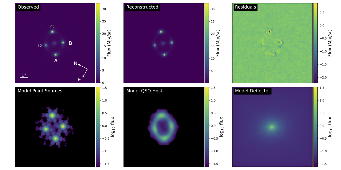
Figure 1: Example results of the image fitting procedure for J1537-3010 in the F560W band. This example shows each of the components used in the image fitting procedure, the lensed emission from the quasar that appears as point sources, the lensed extended emission from the quasar host galaxy, and light from the deflector galaxy. The top left panel shows the observed image, the top center shows the best-fit model, and the top right shows the residuals. The bottom panels show the individual model components.

3.4 Measurement uncertainties

We adopt the flux ratio measurement uncertainties based on the testing of Nierenberg et al. (2023). If the surface brightness of the lensed quasar host galaxy at the location of the point sources is greater than $\sim 50\%$ of the PSF fluxes, then we assume approximately 6% flux-ratio uncertainties. If we have to include the lensed quasar host galaxy in the model but it is fainter than $\sim 50\%$ of the PSF fluxes, we assume 2% flux-ratio uncertainties. If there is no detection of the lensed quasar host galaxy, then we assume 1% flux-ratio uncertainties. We adopt 0$\aas@@fstack{\prime\prime}$005 position uncertainties based on comparisons between our measured image positions and previously published observations of these systems with HST (Schmidt et al., 2023; Shajib et al., 2019; Glikman et al., 2023; Nierenberg et al., 2020).

For the system J1042, we adopt different uncertainties. This system has a pair of images with a flux ratio ranging from about 10:1 in F560W to 4:1 in F2550W, and a separation of only 0$\aas@@fstack{\prime\prime}$5, which is smaller than the PSF FWHM (0$\aas@@fstack{\prime\prime}$591, 0$\aas@@fstack{\prime\prime}$803) in F1800W and F2550W respectively. A potential concern is that if the PSF properties vary systematically with brightness (e.g. the brighter-fatter effect, Argyriou et al., 2023) over this dynamic range, measuring the fluxes with a fixed PSF for all four images may yield a systematic bias. To check this, we performed a fit to the real F2550W data allowing the PSF to vary for each image, and found no trend between the inferred jitter_sigma and the image brightness. The inferred jitter_sigma varied at the 10% level between images, although there was no trend with image flux. This variation is enough to make a significant difference in the measured image fluxes relative to holding this parameter fixed in the fitting. However, to be cautious, for this system we adopt a 10% flux-ratio uncertainty for image B in all filters, and a 5% flux-ratio uncertainty for the other images. Due to the small image separation and large flux differences, we also adopt larger astrometric uncertainties of 0$\aas@@fstack{\prime\prime}$01 for this system.

A new MIRI calibration pipeline was released subsequently to the analysis of Nierenberg et al. (2023), with significant changes to the estimated zero-points, as well as estimates of the zero-point uncertainties. These calibrations also now account for the change in MIRI throughput over the observation period. Although these uncertainties are typically very small $<1\%$, given our quasar fluxes, the absolute image flux uncertainty is likely dominated by PSF modelling uncertainties. We adopt 10% uncertainties on the absolute flux calibration based on the estimates of Nierenberg et al. (2023). The absolute flux uncertainty is relevant for the spectral energy distribution fitting, in which we isolate light coming from specific physical regions of the quasar, as described in Section 5. In our final DM analysis paper for the full sample, we will explore how refining this uncertainty estimate would impact our DM inference.

4 Results of image fitting

The measured image positions and flux ratios of the point sources are presented in Table 2. We provide the flux ratios in the bluest (F560W) and reddest (F2100W or F2550W) filters. In Figure 2 we show how the flux ratios vary as a function of wavelength. We also provide the inferred point source fluxes for all wavelengths in Table  4.

The parameters of the extended emission can be found in Table 5, the parameters of the source are found in Table 6, and the parameters of the galaxy and galaxy satellite light are found in Table 7.

With the exception of J1606 and J1042, all the lenses had extended emission from the lensed source galaxy in the bluest filter, F560. J0607, J1537, and J1606 had extended emission from lensed source galaxy in the reddest filters (F2100W for J0607 and J1537, and F2550W for J1606). All of the lenses with source light detected in the reddest filter have sources with redshift less than 2, and the reddest filter corresponds to $\sim$ 8–10 $\mu$m rest-frame for these systems. The corresponding physical sizes are $\sim$1–3 kpc, however we caution that these values are inferred with a lens modelling procedure optimized to accurately measure the point source image positions and flux ratios, and we leave a more robust inference of the properties of the extended source light to a separate work.

Figure 2 shows that many of the lenses have chromatic variations in the flux ratios. This is due to the fact that at bluer wavelengths, the quasar spectral energy distribution becomes dominated by light from the quasar accretion disk, which is small enough to be microlensed (Sluse et al., 2013). In the following section, we describe how we use SED fitting to account for possible microlensing of physically smaller regions in the light source.

5 SED Fitting

As described by Nierenberg et al. (2023), our goal is to measure the light emitted from the ‘warm dust’ region of the quasar, which is large enough to avoid contamination from microlensing while still being small enough to be sensitive to low-mass halos. Even the reddest MIRI filter contains some amount of contamination from the quasar ‘hot dust’ component. We account for this by fitting the spectral energy distribution (SED) of the quasars based on the four image bands. This procedure is nearly identical to the one presented by Nierenberg et al. (2023), which follows Sluse et al. (2013) by modelling the quasar with a power-law continuum, hot dust blackbody, and warm dust black body. The continuum power-law models emission from the quasar’s accretion disk and the two blackbody models represent emission from the warm and hot dust regions of the quasar. We do not include emission lines such as polycyclic aromatic hydrocarbons since their contribution to the broadband flux is expected to be below percent level for our quasar sources given the MIRI band pass widths  (e.g. Tommasin et al., 2010; Jensen et al., 2017; García-Bernete et al., 2022). The SED fitting gives us a way to propagate possible microlensing contamination into flux-ratio uncertainties, with physically motivated priors on how the different SED components might vary.

The temperature and normalization of the warm dust blackbody component for image A, as well as the flux ratios for the warm dust component in the other images (B/A, C/A, D/A) are all independent parameters that are free to vary. To account for the fact that both the accretion disk and the hot dust region are small enough that they can be microlensed, the amplitude of each of the components in each image is independent and free to vary. Further, the slope of the continuum power-law component was free to vary between the different images, also to account for microlensing. This parameterization also accounts for the intrinsic variability of the accretion disk’s luminosity, which can vary on timescales shorter than the time delay between the lensed images (Schmidt et al., 2023).

We impose priors on several of the SED properties based on the population study by Hernán-Caballero et al. (2016). From this, the temperature of the warm dust region was allowed to vary between 100 and 800 K. The temperature of the hot dust region was allowed to vary between 900 and 1600 K. Hernán-Caballero et al. (2016) found that the flux at 3 $\mu$m coming from the accretion disk contributed a maximum of 20% to the total. We relax this limit given the possibility of differential microlensing between the accretion disk and hot torus and allow an upper limit of 60% on the fraction of flux coming from the accretion disk at this wavelength.

We constrain our model with both the likelihood that the model can reproduce the absolute fluxes for image A in each filter, as well as the likelihood that the model can reproduce the flux ratios of the other images relative to A in each filter. We transform the model SEDs into broadband fluxes following Gordon et al. (2022). We calculate the posterior probability distribution using emcee (Foreman-Mackey et al., 2013).

6 Results of SED fitting

The warm and hot dust flux ratios inferred from the SED fitting are provided in Table 2. Figures showing sample SEDs drawn from the posterior, can be found in the supplementary materials (Appendix E). For lower redshift sources, with $z<2$, the inferred warm dust flux ratios are virtually identical to the flux ratios measured in the reddest band. For some of the higher redshift lenses (e.g., J0659, and J1042), small and statistically insignificant differences in the flux ratios between the reddest filter and the inferred warm dust appear, at the 1 $\sigma$ level. Figure 2 shows the warm dust flux ratios plotted as a band indicating the 68% confidence interval from the SED fitting. In this figure we also show the narrow-line ([OIII], 4969$+$5007 Å doublet) flux ratios measured by Nierenberg et al. (2020) for four of the lenses. The nuclear narrow-line emission is not resolved in these lenses, but is more extended than the warm dust region (e.g. Müller-Sánchez et al., 2011), raising the possibility that a low mass perturber could differentially magnify the two regions, and this is a possible explanation for the difference in measured flux ratios for the case of J0405. The other three lenses show consistent flux ratios between warm dust and narrow-line emission. In future work, we will investigate the probability of differential magnifications for these systems.

Our inference allows for virtually any amount of microlensing of the hot dust, thus we obtain weak constraints on the flux ratios in the hot dust for many of our lenses particularly at lower redshifts where all four JWST filters are redward of 2 microns rest frame. At high redshifts, this is better constrained, and we detect differential microlensing of the hot dust relative to the warm dust for J0405 (image B), J0607 (image A), J1537 (image C). The microlensing of the hot dust could be better constrained if more realistic priors were used for, e.g., the relative amount of microlensing allowed for the continuum emission compared to the hot dust, or with microlensing simulations of the accretion disk and hot dust (e.g. Sluse et al., 2013).

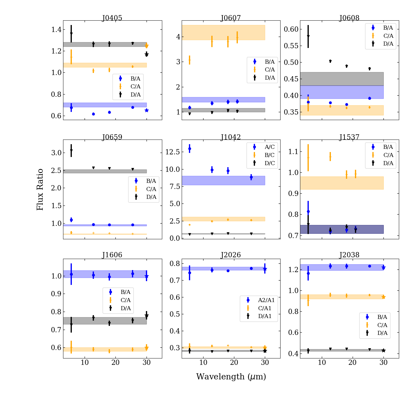
Figure 2: Flux ratios as a function of wavelength for the nine lenses in this study. When available we also include [OIII] (4969$+$5007 Å doublet) flux ratios, plotted arbitrarily as stars at 30$\mu$m with the color corresponding to the same color as the MIRI flux ratio color scheme. Filled bands show the 68% confidence interval for the warm-dust flux ratios. Wavelength dependence in the flux ratios (chromaticity), indicating microlensing by stars, is seen for most systems except J1606, J2026, and J2038. The two reddest filters are always consistent within $\sim$1 $\sigma$, showing the decreased effect of microlensing at these wavelengths. Warm dust and [OIII] are emitted from two different size scales and are not expected to be microlensed but may show differential lensing effects from small subhalos depending on the subhalo masses and locations.

Lens	image	dRAa	dDeca	F560W Flux Ratio	Hot Ratio	Reddest Ratio b	Warm Ratio	[OIII] Ratio
J0405	A	1.065	0.325	1	1	1	1	1
	B	0	0	0.68$\pm 0.04$	0.58${}^{+0.03}_{-0.07}$	0.68 $\pm 0.01$	0.70$\pm$0.02	$0.65\pm 0.04$
	C	0.721	1.161	1.14$\pm$0.07	0.97${}^{0.06}_{-0.1}$	1.06 $\pm 0.02$	1.07$\pm$0.02	$1.25\pm 0.03$
	D	$-0.158$	1.022	1.36$\pm$0.08	1.19${}^{0.07}_{-0.1}$	1.27 $\pm 0.03$	1.26$\pm$0.02	$1.17\pm 0.04$
J0607	A	0	0	1	1	1	1
	B	0.140	1.133	1.18$\pm$0.07	1.02${}^{+0.2}_{-0.5}$	1.42 $\pm$0.08	1.49${}^{+0.1}_{-0.09}$
	C	$-0.321$	1.531	3.07$\pm 0.2$	2.7${}^{+0.6}_{-1}$	3.97 $\pm$0.2	4.17$\pm$0.3
	D	$-1.282$	0.720	0.93$\pm 0.06$		0.7${}^{+0.2}_{-0.4}$	1.03 $\pm$0.06	1.07${}^{+0.08}_{-0.07}$
	G2	0.636	0.965
J0608	A	0	0	1	1	1	1
	B	0.613	0.603	0.38$\pm$0.02	0.36$\pm$0.01	0.391$\pm 0.004$	0.41$\pm$0.02
	C	1.228	-0.273	0.37$\pm$0.02	0.36$\pm$0.01	0.364$\pm 0.004$	0.36$\pm$0.01
	D	0.156	-0.394	0.58$\pm$0.03	0.51$\pm$0.03	0.479$\pm 0.005$	0.45$\pm$0.02
J0659	A	0	0	1	1	1	1
	B	$-4.665$	$-0.335$	1.10$\pm$0.07	0.99$\pm$0.04	0.96 $\pm 0.01$	0.94$\pm$0.02
	C	$-0.979$	2.892	0.73$\pm$0.04	0.74$\pm$0.03	0.700 $\pm 0.007$	0.69$\pm$0.01
	D	0.084	1.903	3.1$\pm$0.2	2.7$\pm$0.1	2.53 $\pm 0.03$	2.47$\pm$0.05
	G2	$-1.375$	2.442
J1042	A	0	0	13.0$\pm 0.6$	10$\pm$3	8.8$\pm 0.4$	8.4${}^{+0.6}_{-0.7}$
	B	-0.147	-0.565	1.9$\pm 0.2$	1.9$\pm$0.8	2.6$\pm$0.3	2.8$\pm$0.3
	C	-0.817	-0.914	1	1	1	1
	D	-1.584	0.546	0.57$\pm$0.03	0.6$\pm$0.1	0.63 $\pm 0.03$	0.65$\pm 0.04$
J1537	A	0	0	1	1	1	1
	B	-1.993	-0.329	0.81$\pm 0.05$	0.68${}^{+0.05}_{-0.1}$	0.73$\pm 0.01$	0.73$\pm$0.02
	C	-2.848	1.644	1.07$\pm$0.06	1.16${}^{+0.1}_{-0.06}$	0.99$\pm 0.02$	0.95$\pm$0.03
	D	-0.750	1.763	0.75$\pm$0.05	0.70${}^{+0.04}_{-0.08}$	0.73$\pm 0.01$	0.73$\pm$0.02
J1606	A	0	0	1	1	1	1	1.00$\pm 0.03$
	B	-1.621	-0.592	1.0$\pm 0.06$	0.98$\pm$0.06	1.01	1.01$\pm$0.02	1.00$\pm 0.03$
	C	-0.792	-0.905	0.60$\pm 0.04$	0.57$\pm$0.04	0.59	0.59$\pm$0.01	0.60$\pm 0.02$
	D	-1.129	0.152	0.73$\pm 0.04$	0.76$\pm$0.05	0.75	0.75$\pm$0.02	0.78$\pm 0.02$
J2026	A1	0	0	1	1	1	1	1.00$\pm$0.02
	A2	0.252	0.219	0.74$\pm 0.04$	0.75$\pm 0$.03	0.772 $\pm 0.008$	0.77$\pm$0.01	0.75$\pm$0.02
	B	-0.164	1.431	0.31$\pm 0.02$	0.31$\pm$0.01	0.303$\pm 0.003$	0.302$\pm$0.005	0.31$\pm$0.02
	C	-0.733	0.386	0.28$\pm 0.02$	0.28$\pm$0.01	0.280$\pm 0.003$	0.282$\pm$0.004	0.28$\pm$0.02
J2038	A	0	0	1	1	1	1	1$\pm$0.01
	B	2.307	-1.707	1.16$\pm 0.07$	1.0${}^{+0.2}_{-0.5}$	1.23$\pm$0.01	1.22$\pm$0.03	1.16$\pm$0.02
	C	0.796	-1.678	0.91$\pm 0.05$	0.8${}^{+0.2}_{-0.3}$	0.96$\pm 0.01$	0.94$\pm$0.02	0.92$\pm$0.02
	D	2.178	0.384	0.42$\pm 0.03$	0.34${}^{+0.08}_{-0.2}$	0.438$\pm 0.004$	0.43$\pm$0.01	0.46$\pm$0.01

Table 2: Results for image fitting and SED fitting. $a$) Image position uncertainties are estimated to be 0$\aas@@fstack{\prime\prime}$005 for all systems except for J1042, which we estimate has 0$\aas@@fstack{\prime\prime}$01 position uncertainties, as described in Section 3.3 $b$) Flux ratio of reddest filter, either F2550W or F2100W as listed in Table 4.

7 Warm Dark Matter Constraint

As discussed in the Introduction, the flux ratios of gravitationally lensed quasars can be used to measure the properties of dark matter. In this work, we combine our measurements of the quasar warm dust with previous measurements of quasar flux ratios to measure the half-mode mass ($M_{\rm hm}$) of the WDM halo mass function. We follow the procedure of Gilman et al. (2020a, 2019) with several updates. For convenience to the reader, we summarize some of the key parts of this analysis here. We begin in Subsection 7.1 by describing the full sample of lenses included in this dark matter constraint. In Subsection 7.2 we describe the model of mass distribution of the lenses that we need to marginalize over in order to calculate the constraint on the DM parameters. We describe our model for the mass function of field halos in Subsection 7.4, and for the subhalos in Subsection 7.5. In Subsection 7.6 we summarize the Approximate Bayesian Computing (ABC) method we use to infer the relative probability of different DM models.

7.1 Full Lens Sample

In addition to the lenses with warm dust flux ratios presented here, we add lenses that have flux ratio measurements that meet the following criteria: 1) flux ratios measured at a wavelength that is not thought to be affected by microlensing (either radio, microwave, or narrow-line emission), 2) a single, simple deflector galaxy that does not have an apparent disk. Beyond the current sample, five gravitational lenses met these criteria, four of which have narrow-line flux ratios (Nierenberg et al., 2017, 2020), and one lens with a CO spectral line measurement Stacey & McKean (2018). A summary of information about the additional lenses is provided in Table 9.

7.2 Macromodel Parameters

The smooth mass distribution of the lens is modelled as a PEMD and external shear. We further generalize this mass model with third and fourth order azimuthal multipoles, to account for the observed boxiness and diskiness of galaxies, specifically by using measurements from Hao et al. (2006). Note that during the DM inference, we do not use any of the main lens model information we derive when measuring the image fluxes as our analysis of the imaging data is focused solely on accurate measurement of the image fluxes. This is conservative and in a future work, will combine constraints from the imaging data using the method of Gilman et al. (2024).

We sample the PEMD power law slope from a Gaussian prior distribution with $\gamma=2.0\pm 0.1$. Multipoles are included in the convergence concentric with the PEMP centroid using:

$$\kappa_{m}(r,\phi)=\frac{a_{m}\theta_{E}}{r\sqrt{q}}\cos(m(\phi-\phi_{m})),$$ (1)

where $\theta_{E}$ is the Einstein radius, $q$ is the axis ratio of the PEMD, and $r$ is the projected separation from the main deflector mass centroid. The prefactor $\theta_{\rm{E}}/\sqrt{q}$ rescales the physical amplitude of these terms such that the observed shape of the iso-density contours depends only upon $a_{m}$. The priors that we implement for these terms are based on the observed shapes of elliptical galaxies (Hao et al., 2006). We adopt a Gaussian prior for $a_{3}/a$ with mean 0.0 and standard deviation 0.005, as well as for $a_{4}/a$ with mean 0.0 and standard deviation 0.01, and we use a uniform prior for $\phi_{3}$ that ranges from $-\pi/6$ to $\pi/6$. For $\phi_{4}$, we allow it to be uniform in the range $-\pi/8$ to $\pi/8$ for $a_{4}/a<0.02$ and keep it fixed to 0 for $a_{4}/a>0.02$. This prior is conservative, as it allows for more freedom for intermediate values of $0.01>a_{4}/a>0.02$, relative to what is actually observed in galaxy light distributions.

When additional companion galaxies are located within $\sim$5 arcseconds of the lensed images (in other filters), we include additional mass components at the location of the light centroid. We assume these objects have Singular Isothermal Sphere (SIS) mass profiles. Unless a redshift has been measured for these systems, we assume they are at the redshift of the main deflector. We estimate their masses based either on their luminosities, or in the case of J0607, by their estimated masses during the lens modelling. This perturber was massive enough to slightly deform the lensed arcs in these systems. For the DM inference, we adopt a uniform prior for the perturber masses centered at the best-fit Einstein radius from our lens modelling with a factor of two mass uncertainty.

7.3 Source Properties

We model the sources in our simulations as Gaussians with a width set by a source size parameter. For our warm dust flux ratios, we draw the source size from a uniform distribution in the range 1-10 pc (Burtscher et al., 2013; Leftley et al., 2019). For our lenses with narrow-line flux ratios, we draw the source size from a uniform distribution in the range 40-80 pc (Müller-Sánchez et al., 2011; Nierenberg et al., 2014, 2017). For J0414, we use the source size of 60 pc as taken from Stacey et al. (2020).

7.4 Field halo mass function

We use a standard cosmology of $\Omega_{\rm m}=0.28$, $\sigma_{8}=0.82$ $h=0.7$ from Hinshaw et al. (2013) when calculating the distribution of halos in CDM (e.g. to calculate a CDM transfer function and CDM halo mass function), and use a halo mass definition of $M_{200}$ calculated with respect to the critical density of the Universe at the halo redshift. For subhalos (see Section 7.5), we define their mass at infall using the same definition. All models discussed in this and following section are implemented for lensing analyses with the open-source software pyHalo (Gilman et al., 2020a).

We model the line-of-sight halo mass function as

$$\frac{d^{2}N}{dMdV}=\delta_{\rm{LOS}}\left(1+\xi_{\rm 2halo}\left(M_{\rm{host},z}\right)\right)\frac{d^{2}N}{dMdV}\bigg{|}_{\rm{ST}}$$ (2)

where $M_{\rm{host}}$ is the host halo mass, and $\frac{dN}{dMdV}|_{\rm ST}$ is the mass function model presented by Sheth et al. (2001). The term $\xi_{2\rm{halo}}$ accounts for correlated structure around the main deflector, as described by Gilman et al. (2019). In our calculation of $\xi_{\rm{2halo}}$, we also include the modification calibrated against N-body simulations by Lazar et al. (2021), which increases the number of halos introduced through this term by a factor of $\sim 2$. $\delta_{\rm LOS}$ is introduced to account for theoretical uncertainties in calculating the normalization of the halo mass function (Despali et al., 2016).

The WDM mass function is calculated as a suppression applied to the Sheth-Torman mass function, with the following fitting formula

$$\frac{d^{2}N_{\rm WDM}}{dMdV}=\frac{d^{2}N_{\rm CDM}}{dMdV}f_{{\rm{WDM}}}\left(M,M_{\rm{hm}}\right)$$ (3)

where

$$f_{{\rm{WDM}}}\left(M,M_{\rm{hm}}\right)=\left(1+\left(\alpha\frac{M_{\rm hm}}{M}\right)^{\beta}\right)^{\gamma}$$ (4)

with $\alpha=2.3$ $\beta=0.8$ $\gamma=-1.0$ (Lovell, 2020). We model halos as truncated Navarro-Frenk-White (NFW) profiles (Navarro et al., 1997)

$$\rho\left(r\right)=\frac{\rho_{s}}{x\left(1+x\right)^{2}}\frac{\tau^{2}}{x^{2}+\tau^{2}}$$ (5)

where $x\equiv r/r_{s}$, $\tau\equiv r_{t}/r_{s}$, $r_{s}$ is the halo scale radius, and $r_{t}$ is a truncation radius. For field halos, we set $r_{t}=r_{\rm{50}}$, where $r_{50}$ is the radius that encloses 50 times the critical density, in order to keep the mass rendered along the line of sight finite.

In CDM, we calculate $r_{s}$ for a halo of mass $m$ using the concentration–mass relation presented by Diemer & Joyce (2019). To model the concentrations of WDM halos, we use the fitting function given by Bose et al. (2016)

$$\frac{c_{\rm WDM}(M,z)}{c_{\rm CDM}(M,z)}=(1+z)^{\beta(z)}\left(1+60\frac{M_{\rm hm}}{M}\right)^{-0.17}$$ (6)

where $\beta(z)=0.026z-0.04$. The suppression of the concentration of WDM halos results from the delayed formation time of structure in these models Wechsler et al. (2002); Ludlow et al. (2014).

7.5 Subhalos

When a halo in the field accretes onto the host halo of the main deflector, it decouples from the background density of the Universe and evolves in the gravitational tidal field of the host. This section details how we model the population of main deflector subhalos, and implements several improvements relative to the work by Gilman et al. (2020a).

7.5.1 The projected number density of main deflector subhalos

We model the infall subhalo mass function with a mass function of the form (Gilman et al., 2020a)

$$\frac{d^{2}N_{\rm sub}}{dMdA}=\frac{\Sigma_{\rm sub}}{10^{8}}\left(\frac{M}{10^{8}}\right)^{\alpha}\mathcal{F}(M_{\rm{host}},z)f_{{\rm{WDM}}}\left(M,M_{\rm{hm}}\right),$$ (7)

where $\Sigma_{\rm sub}$ and $\alpha$ are the normalization and logarithmic slope of the subhalo mass function at infall. The slope $\alpha$ is taken to be in the range -1.95 to -1.85, as found in simulations (Springel et al., 2008; Fiacconi et al., 2016). The function $\mathcal{F}$, given by

$$\log\mathcal{F}(M_{\rm{host}},z)=k_{1}\log\left(\frac{M_{\rm{host}}}{10^{13}M_{\odot}}\right)+k_{2}\log\left(z+0.5\right)$$ (8)

which factors out the evolution of $\Sigma_{\rm{sub}}$ with host halo mass and redshift such that we can combine inferences of $\Sigma_{\rm{sub}}$ from lenses with different host halo masses and different redshifts. Based upon an updated calibration of the semi-analytic model galacticus (Benson, 2012), we use $k_{1}=0.5$ and $k_{2}=0.3$ (Gannon et al, in prep). For this analysis, we assume all of the deflectors have the strong lens population average halo mass $M_{\rm{host}}=10^{13.3}$ M_⊙ measured by Lagattuta et al. (2010). We place lenses that do not have spectroscopic or photometric redshift measurements at $z=0.5$. This uncertainty primarily affects the inference through the dependence of the subhalo population on the host mass and, to a much smaller extent, the host redshift. Using Equation 8, the number of subhalos varies by a factor of $2$ when varying the halo mass in the range $M_{\rm halo}\in 10^{13},10^{13.6}$ and by a factor of 1.2 when varying the lens redshift over the range $z\in 0.3,1.0$. Both of these factors are much smaller than the 1.5 dex range used for the $\Sigma_{\rm sub}$ prior.

7.5.2 The evolved subhalo mass function

By definition, the amplitude of the projected infall subhalo mass function (Equation 7) does not depend on tidal stripping and heating. However, this is not what we measure with strong lensing. Instead, lensing measures the evolved subhalo mass function in addition to the mass function of halos along the line of sight. The evolved subhalo mass function depends on tidal stripping and heating by the host halo and the main deflector galaxy. A common approach to modeling the evolved subhalo mass function is to fit a mass function to the output of numerical simulations, and draw subhalo masses from this model. The drawback of this approach is that it changes the mass definition of subhalos, and formally requires the re-calibration of the concentration–mass relation for these objects. It also obscures the connection between the physical properties of subhalos at infall, which depend on DM physics, and the properties of the evolved subhalo mass function. Put differently, this approach conflates the modification to halo density profiles from the cosmological effects of DM free-streaming with tidal stripping and heating by a central potential.

To model the evolved subhalo mass function, we derive a transfer function that establishes a probabilistic mapping between properties of halos at infall and the bound mass of a subhalo at the time of lensing. We can phrase the task at hand as assigning bound masses to subhalos, or equivalently, assigning truncation radii $r_{t}$ (Equation 5), to individual subhalos in such a way that the statistical properties of the evolved subhalo population match the statistical properties of evolved subhalo populations output by numerical simulations. This approach assumes that the lensing signal depends primarily on the tidal truncation $r_{t}$, and not on the less substantial evolution of other structural parameters, such as $\rho_{s}$ and $r_{s}$, that can in principle also change due to tidal heating.

The structural parameters of NFW halos evolve along ‘tidal tracks’ (Errani & Navarro, 2021; Du et al., 2024), a self-similar trajectory along which halo density profiles evolve in a tidal field. The rate at which halos traverse tidal tracks depends on the concentration of the halo and the concentration of the host, and the position of a halo along the tidal track depends on the elapsed time since infall (Stücker et al., 2023). Because strong lensing probes a region projected down the center of the host halo that is very small compared to the virial radius of the host, the bound mass function in this regime does not have a strong dependence on the projected two-dimensional position of a subhalo (Xu et al. 2015; Gannon et al. in prep). Thus, we will seek a mapping to the bound mass of subhalos only in terms the subhalo concentration at infall, $c$, the host halo concentration, $c_{\rm{host}}$, and the time since infall, $t_{\rm{infall}}$. As the number of subhalos is typically $\mathcal{O}\left(100\right)$, from the central limit theorem we model the probability distribution of $m_{\rm{bound}}/m_{\rm{infall}}$ as a Gaussian, and introduce dependence on $c$, $c_{\rm{host}}$, and $t_{\rm{infall}}$ through the mean and standard deviation, i.e. $m_{\rm{bound}}/m_{\rm{infall}}\sim p\left(\mu\left(c,c_{\rm{host}},t_{\rm{infall}}\right),\sigma\left(c,c_{\rm{host}},t_{\rm{infall}}\right)\right)$. From $m_{\rm{bound}}/m_{\rm{infall}}$, we can then calculate $r_{t}$ given the infall mass of the subhalo using Equation 5.

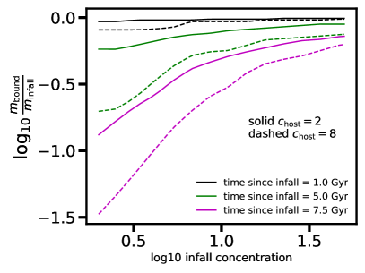
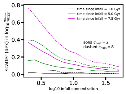
Figure 3: The mean (top) and standard deviation (bottom) of the bound mass of an individual subhalo as a function of the infall concentration, the time since infall, and the host halo concentration.

To compute the functions $\mu\left(c,c_{\rm{host}},t_{\rm{infall}}\right)$ and $\sigma\left(c,c_{\rm{host}},t_{\rm{infall}}\right)$, we perform a series of calculations with galacticus in which we inject individual subhalos into a static host potential, and evolve them for $t_{\rm{infall}}$ Gyr. Subhalos are initially placed at the virial radius of the host, and are assigned initial orbital parameters by drawing from the distribution of subhalo infall orbits measured in cosmological N-body simulations by Jiang et al. (2015). Each subhalo is then evolved under the physical models (including dynamical friction, tidal heating, and tidal stripping) described by Yang et al. (2020), Benson & Du (2022), and Du et al. (2024). We then record the bound mass of the subhalo at the end of the simulation, and repeat the calculation thousands of times for each cell on a grid of $c_{\rm{host}}$, $c$, and $t_{\rm{infall}}$. We determine $\mu$ and $\sigma$ for the distribution of bound subhalo masses in each cell, and perform a spline interpolation of the $\mu$ and $\sigma$ values to derive continuous functions for these quantities. The $\mu$ and $\sigma$ functions have a negligible dependence on infall subhalo mass.

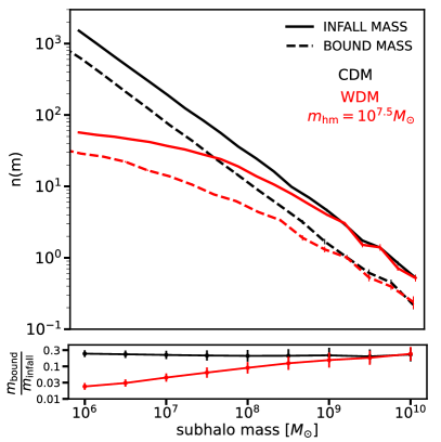
Figure 4: Infall and bound subhalo mass functions in CDM (black) and for a WDM model with $m_{\rm{hm}}=10^{7.5}M_{\odot}$. The top panel depicts the median and scatter in the number of halos averaged over 100 realizations according to the infall mass definition (solid lines) in comparison with the number of halos binned according to their bound mass calculated according to the procedure discussed in Section 7.5. The bottom panel shows the average bound mass of surviving subhalos as a function of their infall mass, illustrating the differential suppression of the WDM bound subhalo mass function due to the suppression of halo concentrations in WDM and the dependence on the tidal stripping model on subhalo concentration at infall (see Equation 6 and Figure 5)

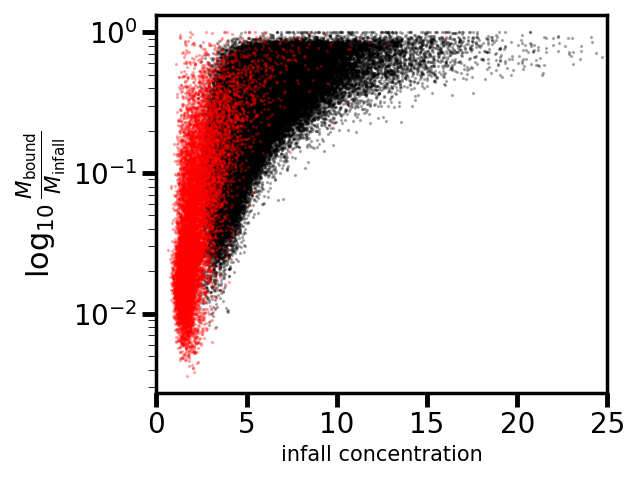
Figure 5: The distribution of infall concentration versus bound mass for a CDM subhalo population (black) and WDM subhalo population with $m_{\rm{hm}}=10^{7.5}M_{\odot}$ (red) using the tidal truncation model discussed in Section 7.5.

Figure 3 shows the functions for $\mu$ and $\sigma$ that result from these calculations. The mean captures the leading-order effects of tidal stripping, reflecting the fact that the amount of mass loss depends, to leading order, on $c$, $c_{\rm{host}}$, and $t_{\rm{infall}}$. The standard deviation accounts for all other effects that we do not explicitly include in the model, such as the orbital pericenter of subhalo orbits. The average bound mass relative to infall mass decreases for lower infall concentration, reflecting the fact that less concentrated subhalos lose mass more rapidly than more concentrated subhalos. The scatter in bound masses includes the dependence on orbital pericenters. The scatter increases at lower infall concentration because subhalos with small pericenters get rapidly disrupted if they have low concentrations, while subhalos that appear in projection near the Einstein radius but have large orbital pericenters retain most of their mass. In contrast, more concentrated subhalos are more resilient to tidal effects, and therefore they have a weaker dependence on the orbital pericenter, which is a latent variable in these calculations. The model predicts that halos accreted at earlier times lose more mass than recently-accreted subhalos. We assign values of $t_{\rm{infall}}$ to individual subhalos in pyHalo using the distribution of infall times predicted by galacticus for subhalos that appear within a 20 kpc aperture of the host center.

Figure 4 shows the result of applying this tidal stripping model to subhalo populations in CDM and WDM generated with pyHalo. In CDM, the model predicts halos lose $\sim 70\%$ of their mass on average, with little to no dependence on the infall mass. On the other hand, in WDM the amplitude of the bound mass function becomes increasingly suppressed at lower masses due to the suppressed halo concentrations on scales $m\lesssim m_{\rm{hm}}$. Figure 5 more clearly shows the effect of infall concentration on the distribution of subhalo bound masses. The explicit dependence on infall concentration introduces an additional lever with which to distinguish between CDM and WDM models, as WDM subhalo populations will systematically have a lower bound mass function amplitude due to the explicit dependence on infall concentration, which becomes suppressed in WDM models (Equation 6).

In Figure 6, we compare the cumulative distribution for the flux ratio of a lensed image for varying values of $\Sigma_{\rm{sub}}$, with no line of sight halos included. These simulations are for a lens with a halo mass of $10^{13}$ M_⊙ at a redshift of 0.5, for subhalos with bound masses between $10^{7}$ and $10^{8}$ M_⊙. One should interpret the width of the distribution of flux ratios (or the slope of the CDF) as a proxy for the lensing signal that statistically differentiates various dark matter models. As expected, as $\Sigma_{\rm{sub}}$ increases, the width of the distribution also increases. The yellow dashed line shows the cumulative distribution of flux ratios for subhalos with bound masses and concentrations consistent with direct output from the galacticus simulations. The prior on $\Sigma_{\rm{sub}}$ is large enough to accommodate a large range of theoretical uncertainty on the properties of dark matter subhalos. We emphasize that these distributions are for flux ratios produced only by subhalos, which make up only about 10-20% of the halos near the lensed images in projection, thus differences in the flux ratio distributions for full realizations of subhalos and line-of-sight halos will depend significantly less on $\Sigma_{\rm{sub}}$ than the results shown here.

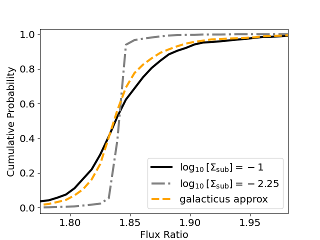
Figure 6: Cumulative probability distribution of flux ratios produced by dark matter subhalos for a lens with halo mass $10^{13}$ M_⊙ at redshift 0.5 for different choices of the normalization of the subhalo mass function, $\Sigma_{\rm sub}$. Comparison of the orange, grey and black lines shows that the prior on $\Sigma_{\rm{sub}}$ used in our measurement encompasses predictions from galacticus, while also accommodating a broad range of theoretical uncertainties. In reality, subhalos make up only $10-20\%$ of the halos in projection near lensed images, so this figure exaggerates the impact of uncertainties in the properties of subhalos.

7.6 The calculation of the likelihood function

Here we describe the statistical procedure we use to constrain WDM using the flux-ratio measurements of the warm dust region. This procedure follows the methodology described in Gilman et al. (2024) (see also Gilman et al. (2020a)), and yields accurate and unbiased results in both WDM and CDM mock data sets.

Our methods require simulation-based likelihoods because the fluxes of each image depends on the specific realization of DM structure; the model is stochastic. Different parameter values for the DM model predict different distributions of flux ratios. The colder the DM model, the more halos the model predicts, and thus the wider the distribution of predicted flux ratios. These distributions of flux ratios are very correlated and non-Gaussian and so to estimate the likelihood of observing a set of measured flux ratios, given a set of model parameters, we use Approximate Bayesian Computing (ABC) (Rubin, 1984; Marin et al., 2011; Lintusaari et al., 2017). The ABC method works first by sampling parameters from the prior, computing the observables for each sample, and then selecting the samples that best fit the data, as defined by a summary statistic. For the parameters of our DM model, $\log_{10}M_{\rm hm}$, $\log_{10}\Sigma_{\rm sub}$, and $\delta_{\rm LOS}$ are sampled from uniform priors with ranges $\in{4.0,10.0}$, $\in{-2.5,-1.0}$, $\in 0.8,1.2$, respectively and $\alpha$ has a Gaussian prior with $-1.90\pm 0.05$. The prior on $\Sigma_{\rm sub}$ was chosen to span a wide range centered on the predictions of galacticus, while the prior of $M_{\rm hm}$ was chosen such that the upper end was the maximum value of the halos we explicitly render with pyHalo while the lower end extends below where we were forecasted to constrain by a few dex. The prior on $\delta_{\rm LOS}$ was chosen to account for theoretical uncertainties associated with calculating the halo mass function Despali et al. (2016). The prior on $\alpha$ was taken from results of N-body simulations (Springel et al., 2008; Fiacconi et al., 2016).

With these parameters, we use pyHalo to populate our lens with DM subhalos and line-of-sight halos, drawn from randomly sampled DM parameters. Halos with masses above $10^{10}M_{\odot}$ are relatively rare, and expected to contain galaxies with absolute magnitudes of approximately $M_{v}\sim-16$ (e.g. Tollerud et al., 2008). Such galaxies are detectable in single orbit Hubble Space Telescope imaging to a redshift of $z\sim 2$ (Koekemoer et al., 2007; Nierenberg et al., 2016). The majority of our systems have such imaging with the exception of J0607 and J0608. For J0607, a luminous companion is detected in the JWST MIRI imaging. When detected, we explicitly include the companions in the lens model as singular isothermal spheres (SIS) assumed to be at the redshift of the main deflector. We include these massive subhalos in J0607, J1042, and J1606.

Given a realization of DM halos, as well as a subset of randomly-sampled macromodel parameters (the slope of the lens mass distribution $\gamma$, the multipole amplitudes $a_{3}$, $a_{4}$, and angles, $\phi_{3}$, $\phi_{4}$) we apply a non-linear solver to the remaining portion of the lens macromodel(Einstein radius $\theta_{E}$, ellipticity, orientation, external shear, and source position) such that the multi-plane lens equation is satisfied for each realization of dark matter subhalos and line-of-sight halos. In the next step, we calculate the flux ratios for a sampled realization of DM halos and macromodel parameters, with source properties sampled as described in 7.3.

Now we can compare the predicted flux ratios, for a given DM halo realization, from a given set of model parameters, to the observed flux ratios. This is the step where the ABC method is relevant. The ABC method approximates a posterior by selecting the parameters from the prior which predict observables close to the data, as measured by a summary statistic. We choose the following summary statistic, $S=\sqrt{\sum_{i}(f_{i,\rm{obs}}-f_{i,\rm{pred}})^{2}}$ where the $f$ variable are the observed and predicted flux ratios and the sum is over the three flux ratios. We choose the 1000 prior samples corresponding to the smallest summary statistic for each lens. The acceptance rates vary between lenses, but this choice typically results in flux ratios that match the data to well-within the measurement uncertainties of the flux ratios. We have verified this way of estimating the posterior probability distribution returns accurate results with mock data sets (Gilman et al., 2024).

We use samana (Gilman et al., 2024) to sample the prior, vary the macromodel parameters, and wrap the functionality of pyHalo and lenstronomy (Birrer & Amara, 2018; Birrer et al., 2021) for the lensing calculations.

8 Results

The results of the ABC inference for these lenses is shown in Fig. 7. There, the posterior indicates that our results constrain the half-mode mass to be below $\log_{10}M_{\rm hm}<7.6$ (posterior odds 10:1, relative to the peak of the posterior). In Table 3, we show the posterior odds for a few additional example values of the half-mode mass.

We use the following equation to interpret our constraints on the half-mode mass as a constraint on the mass of the DM particle,

$$M_{\rm hm}=3\times 10^{8}\left(\frac{m_{\rm WDM}}{3.3\,\rm{keV}}\right)^{-3.33}M_{\odot},$$ (9)

as shown by Schneider et al. (2012, 2013); Vogel & Abazajian (2023). Thus, our constraint on the half-mode mass corresponds to a constraint on the DM particle mass of $m_{\rm WDM}>6.1$ keV (posterior odds 10:1).

$\log_{10}M_{\rm hm}$	$m_{\rm th}$ (keV)	Odds	Gilman 2020a
$7.0$	9.2	3.6	1.2
$7.5$	6.5	8.7	1.6
$8.0$	4.6	24.	3.2
$8.5$	3.2	44.	9.6

Table 3: Posterior odds evaluated for example values of $\log_{10}M_{\rm hm}$. We include a comparison with the odds calculated for the same half-mode masses from  Gilman et al. (2020a).

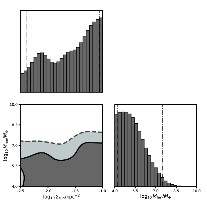
Figure 7: Posterior probability distribution for the DM model parameters $M_{\rm{hm}}$ and $\Sigma_{\rm{sub}}$. The data favors models which yield high amounts of low-mass structure over those that do not. We rule out a half-mode mass greater than $10^{7.6}$M_⊙ (posterior odds 10:1) corresponding to a WDM particle mass of 6.1 keV.

9 Uncertainty Budget

Here we summarize some of the key contributors to the uncertainty budget of our measurement.

9.1 Warm Dust Measurements

The uncertainty associated with the flux ratio measurements was discussed extensively by Nierenberg et al. (2023). Lenses with a bright arc in the reddest filter will have the largest measurement uncertainty ($\sim$6%), while the absolute flux uncertainty of $\sim 10\%$ also contributes through the SED fitting to the measurement uncertainty. With improvements to the PSF model as well as better characterization of the MIRI detector it is possible that the absolute flux uncertainty may be reduced in the future. Typically, however, the inferred warm dust flux ratio uncertainties are dominated by the flux ratio uncertainties in the reddest filter so we do not anticipate this will have a significant affect on the DM measurement based on this data.

9.2 Lens Macromodel

We adopt a uniform prior on the ellipticity and orientation of the macromodel. The multipole moments are drawn from optical measurements of field ellipticals (Hao et al., 2006). Gilman et al. (2024) demonstrated that the inclusion of mass distribution information from the lensed quasar host galaxy from Hubble Space Telescope imaging can directly improve the sensitivity to WDM models by directly constraining the macromodel for each lens. For the sample of mock lenses studied by Gilman et al. (2024), this improved the measurement by a factor of $\sim 3$ in the half-mode mass for a CDM truth for a sample of 25 lenses with HST imaging of the lensed quasar host galaxy relative to a measurement without this information.

9.3 Dark Matter Model

The most significant uncertainties in our DM model are related to the model for tidal stripping of the subhalos. For a typical lens, with source redshift of 1.5, deflector redshift of 0.5 and a halo mass of $10^{13}$ M_⊙, the ratio of subhalos to field halos near the lensed images is approximately 1:5 based on estimates with pyHalo . Although the subhalos are subdominant, they comprise a large enough fraction of the population that uncertainties in modelling must be carefully accounted for. We enable a broad range of $\Sigma_{\rm{sub}}$ values relative to what is seen in simulations of these populations; this reflects our uncertainty in the pre-infall normalization of the subhalo mass function as well as our much larger uncertainty in the amount of tidal stripping that subhalos undergo. Our prior on $\Sigma_{\rm{sub}}$ is chosen to match the bound mass fraction measured from galacticus when the pyHalo tidal stripping model is applied to a population of subhalos. This yields a bound mass fraction which is consistent with not only galacticus but also a range of N-Body simulations (Fiacconi et al., 2016; Griffen et al., 2016; Gao et al., 2012) for halos at this mass. Nadler et al. (2021a) showed that combining luminous satellite galaxies of the Milky Way could provide a constraint on $\Sigma_{\rm{sub}}$, and that a combination of gravitational lensing and luminous satellite counts can provide a stronger constraint on a turnover in the halo mass function than either method on its own. We will incorporate such constraints in a future paper, when we infer the properties of dark matter for the whole sample of lenses.

The model for the suppression of the warm dark matter halo mass function implements the most recent calibration by Lovell (2020). The suppression term (Equation 4) in this model has a logarithmic slope at $m<m_{\rm{hm}}$ of -0.8, relative to the -1.3 logarithmic slope of mass function suppression presented by Lovell et al. (2014) that was used in previous studies (Gilman et al., 2020a; Hsueh et al., 2020). For a given $m_{\rm{hm}}$, the updated model predicts more low-mass halos than the previous WDM fit, which leads to weaker constraints on the free-streaming length for a given dataset.

10 Discussion

By combining our new measurements of the warm dust with the narrow-line and CO measurements, we placed the tightest gravitational lensing constraint to date on a possible turnover in the halo mass function, and thus on free streaming length of warm dark matter.

Our limit is consistent and more stringent than that by Gilman et al. (2020a) which found $M_{\rm{hm}}<10^{7.8}$ $M_{\odot}$ for a sample of 8 lenses with narrow-line flux ratios. The improved limit is a result of several differences with respect to Gilman et al. (2020a). First, the sample is larger, including five lenses that were not part of the previous sample. Thus, we expect that differences in the strength of the constraint will arise from sample variance. Second, we have updated the treatment of tidal stripping of subhalos. Third, the intrinsic source sizes differ in the two works, with the nuclear narrow-line region having a characteristic scale of $\sim 50-80$ pc, and the warm dust region having sizes of order $1-10$ pc; this analysis combines measurements from both source types while the prior measurement used only narrow-line sources. Finally, we have now included flexible higher order multipole perturbations to the macromodel, following Gilman et al. (2024).

Several recent works have highlighted the existence of multipoles in lens galaxy isophotes (e.g. Stacey et al., 2024; He et al., 2024; Cohen et al., 2024; Gilman et al., 2024; Oh et al., 2024), and considered the impact of these features on the measurement of the properties of low mass halos. Gilman et al. (2024) tested the impact of these multipoles on mock simulations of quasar lenses similar to the sample considered in this paper, and demonstrated that it was possible to derive correct constraints on the half-mode-mass for both warm and cold ground truths even in the presence of random, unknown $a_{3}$ and $a_{4}$ multipoles in the deflector macromodels with an appropriate statistical treatment of the problem. Our results in the current work further demonstrate that strong constraints on the nature of dark matter are possible, while simultaneously accounting for multipole deviations in the deflector mass distribution based on measurements of the properties of populations of elliptical galaxies. In Figure 8, we show the joint posterior probability distribution for the multipole amplitudes and the DM half-mode mass for two of the lenses that are typical of our sample, in that there is no significant correlation between a cutoff in the half mode mass and the amplitude of the multipole moments.

Our constraints are comparable to those based on Lyman-$\alpha$ (Viel et al., 2013; Iršič et al., 2017; Villasenor et al., 2023), which correspond to $m_{\rm WDM}>3.3,5.3,3.1$ keV, respectively. Similarly, counting satellite galaxies of the Milky Way provide constraints in the range $m_{\rm WDM}>2.02$ keV (Newton et al., 2021), $m_{\rm WDM}>3.6$–$5.1$ keV (depending on the mass of the Milky Way) (Dekker et al., 2022), and 6.5 keV (Nadler et al., 2021a), and 7.4 keV when combined with strong lenses (Nadler et al., 2021b). Substructure lensing, Milky Way satellite counts, and the Lya forest probe independent scales of the matter power spectrum at different redshifts, so most of the systematic uncertainties are independent. It is reassuring that these probes all disfavor WDM models in similar portions of parameter space and each probe makes the others’ conclusions more robust.

11 Summary

Here we provide a summary of the key results of our paper.

• We present rest-frame mid-IR fluxes measured with JWST MIRI for a sample of 9 lenses. Using SED fitting, we isolate the light coming from the warm dust region. The SED fitting gives inferred warm-dust flux ratios consistent with those measured in the reddest filters, where the effects of microlensing are minimized. All systems show some degree of microlensing in at least one image in the bluest filter relative to the reddest filter, highlighting the importance of having multiband MIRI band imaging.

• We present an updated treatment of subhalo tidal stripping and evolution within the host potential.

• We use the flux ratios of the warm dust region, in combination with previously published flux ratios at other wavelengths, to calculate the posterior probability distribution of the WDM model. We find that the half-mode mass is constrained to be less than $10^{7.6}$ $M_{\odot}$ at posterior odds of 10:1. This corresponds to constraint on the WDM particle mass to be above $m_{\rm WDM}>6.1$ keV.

• Our new limit on the free streaming length of dark matter is the strongest calculated from gravitational lensing to date and improves upon and is consistent with previous results from flux-ratio anomalies (Gilman et al., 2020a). Importantly, by virtue of the larger sample and new measurements, it is more stringent than the previous measurement even if it allows for departures from ellipticity in the mass distribution of the lenses.

• Our new limit is consistent with independent limits based on the Ly-$\alpha$ forest and Milky Way Satellites.

Data Availability

This work was based on JWST MIRI imaging which becomes publicly available after a one-year proprietary period. All software used in the DM inference is publicly available, and intermediate data products may be made available upon reasonable request.

Appendix A Multipoles

To illustrate the effects of multipoles, we show the posteriors for two example lenses in Fig 8. For 0405, we see that the half-mode mass and multipole parameters are uncorrelated and weakly constrained, relative to the prior. For 0659, based on the structure of the 95 $\%$ confidence interval in the joint $a_{4}/a$ and $M_{\rm{hm}}$ distribution, non-zero $a_{4}$ slightly weakens the constraint on $M_{\rm{hm}}$ relative to $a_{4}=0$. This figure clearly illustrates how additional degrees of model freedom affect ones posterior beliefs regarding the allowed values of certain model parameters, in this case the free streaming length.

Distinguishing between various models that could explain the same dataset involves Bayesian model comparison. To illustrate this concept, we have analyzed the fourteen lenses in this work with lens models that only includes $m=3$ and $m=4$ multipole terms. We compute the posterior odds ratio, or Bayes factor, between lens models that include only these multipole terms and with lens models that include both multipoles and substructure (for additional details about these tests, see Appendix B in Gilman et al. (2024)). The posterior odds enables a Bayesian model comparison between two competing models that could both give rise to an observed dataset. These odds can be calculated from simulation-based inference methods by quantifying the frequency with which a the observed dataset emerges from a given model. The joint Bayes factor for the 14 lenses considered in this work exceeds 1,000. This indicates that a lens model that fits the data with substructure is overwhelmingly preferred relative to model that explains the data with only perturbations to the shape of the main deflector. Analyzing the data within the context of the model that includes both sources of perturbation leads to the statements regarding the free-streaming length of dark matter presented in this work.

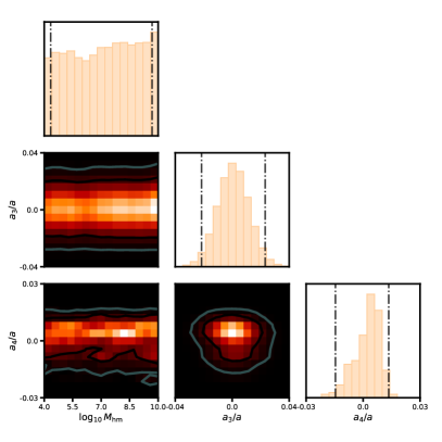
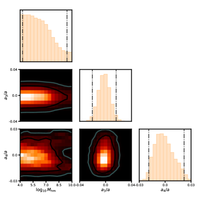
Figure 8: Example posteriors in the space of $M_{\rm hm}$, and the multipole amplitudes, $a_{3}/a$ and $a_{4}/a$, for the individual lenses 0405 (left), and 0659 (right).

Appendix B Image fluxes

Here we provide the measured image fluxes for our systems.

Lens	image	F560W	F1280W	F1800W	F2100W	F2550W
J0405	A	0.365	1.05	1.38		2.66
	B	0.246	0.646	0.871		1.80
	C	0.418	1.07	1.41		2.80
	D	0.497	1.32	1.74		3.37
J0607	A	0.0785	0.161	0.223	0.261
	B	0.0923	0.217	0.313	0.370
	C	0.241	0.613	0.849	1.038
	D	0.03	0.157	0.236	0.269
J0608	A	1.2154	5.5023	6.9931		8.0359
	B	0.46174	2.0791	2.6063		3.1453
	C	0.454099	2.0185	2.5336		2.9256
	D	0.702176	2.7666	3.4098		3.8568
J0659	A	0.131	0.675	0.999		1.237
	B	0.145	0.648	0.953		1.181
	C	0.0963	0.486	0.713		0.867
	D	0.402	1.737	2.556		3.313
J1042	A	5.33	19.98	31.66		42.78
	B	0.797	4.94	8.69		12.74
	C	0.411	2.015	3.24		4.84
	D	0.235	1.26	2.17		3.08
J1537	A	0.0632	0.242	0.386	0.483
	B	0.0515	0.174	0.281	0.353
	C	0.0677	0.260	0.382	0.479
	D	0.0476	0.174	0.285	0.351
J1606	A	0.516	1.817	2.640		4.950
	B	0.521	1.825	2.625		5.010
	C	0.310	1.072	1.530		2.914
	D	0.375	1.389	1.942		3.714
J2026	A1	1.999	8.581	12.59		20.23
	A2	1.488	6.534	9.529		15.62
	B	0.615	2.661	3.936		6.136
	C	0.562	2.382	3.525		5.666
J2038	A	3.799	8.798	15.22		21.36
	B	4.419	10.85	18.74		26.31
	C	3.440	8.434	14.46		20.43
	D	1.608	3.891	6.756		9.362

Table 4: Measured image fluxes in units of mJy

Appendix C Lens Model Parameters

Here we provide the best-fit lens model parameters (Table 5), light parameters, and PSF parameters found in the final step of our fitting, where the point sources are treated as free foreground objects. These macromodels are provided to aid reproduction of our flux-ratio measurements. Given that our goal was to optimize the measurement of the image positions and fluxes, the fact that we do not use the image positions to constrain the lens model in the final fitting step, the ongoing room for improvement in the MIRI PSF models, particularly in F560W which typically has the brightest arc, and therefore the strongest constraint on the lens model, we do not recommend these values should be interpreted as robust physical constraints of the properties of the lenses.

Lens	$\theta_{\rm{E}}$	$\gamma_{p}$	$q$	$\phi$ (degree)	$\gamma_{\rm{ext}}$	$\phi_{\gamma}$ (degree)	dRA	dDec	$\theta_{\rm{G2}}$	dRAG2	dDecG2
J0405	0.72	2.02	0.55	260	0.077	250	0.362	0.542
J0607	0.77	2.00	0.71	142	0.077	143	-0.532	0.717	0.118	0.687	0.984
J0608	0.68	2.00	0.34	184	0.147	182	0.558	0.062
J0659	2.40	2.01	0.57	210	0.010	150	-1.699	0.983
J1537	1.39	2.02	0.89	357	0.133	466	-1.444	0.766
J1606	0.67	1.93	0.47	389	0.154	351	-0.826	-0.451
J2038	1.38	2.33	0.54	305	0.047	365	-0.721	-0.914

Table 5: Best fitting lens model parameters, with the image positions not used in the lens model. Position angles are given in degrees East of North, all other angles are in units of arcseconds. Lens centers given relative to coordinate system in Table 2. Note that lenses 1042, 2026 did not have detected extended arcs in any filter and thus no lens model was applied.

Lens	Filter	rs (arcsec)	ns	nmax	$\beta$ (arcsec)	dRa	dDec
J0405	F560W	0.25	7	5	0.11	0.245	1.282
	F1280W	0.30	0.5	–	–
	F1800W	0.07	1	–	–
J0607	F560W	1.081	5.95	3	0.11	-0.180	0.017
	F1280W	0.318	1.17	–	–
	F1800W	0.314	1.15	–	–
	F2100W	0.306	1.05	–	–
J0608	F560W	0.55	6.00			0.720	-0.468
J0659	F560W	0.21	5.95	–	–	$-2.284$	0.726
J1537	F560W	0.12	1.00			$-1.203$	$-0.254$
	F1280W	0.02	1.00
	F1800W	0.13	1.00
	F2100W	0.16	1.00
J1606	F560W	0.34	1.0			$-0.631$	0.085
	F1280W	0.34	1.0
	F1800W	0.35	0.9
	F2550W	0.36	0.9
J2038	F560W	0.25	1.00			$-$1.060	$-$0.987
	F1280W	0.25	1.00

Table 6: Best fitting source parameters with positions given in the coordinate system of Table 2. The source centroids are restricted to be the same in all filters. Lenses 1042, 2026 and filters which are not listed did not contain a detected lensed quasar host galaxy.

Lens	Filter	Rs (arcsec)	$q$	$\theta$ (degrees)	dRA	dDec	Rs,sat
J0405	F560W	0.16	0.87	0	0.375	0.542
	F1280W	0.04	0.59	-40
J0607	F560W	0.39	0.75	86	-0.549	0.752	0.075
J0608	F560W	0.30	0.44	173	0.453	-0.010
J0659	F560W	0.59	0.95	162	-1.795	0.860
	F1280W	0.27	0.60	172
	F1800W	0.88	0.93	158
	F2550W	–	–	–
J1537	F560W	0.66	0.79	372	-1.434	0.754
	F1280W	1.45	0.52	391
J1606	F560W	0.11	0.41	353	-0.845	-0.395
J2038	F560W	6.95	0.53	308	-0.721	-0.85

Table 7: Best fitting deflector and satellite light parameters with positions given relative to the coordinate system in Table 2. Deflector light centroids are constrained to be the same in all filters. Sérsic indices are held fixed to 4 for the deflector and satellite light.

Lens	Filter	jitter_sigma (arcsec)	T (K)	fa
J0405	F560W	0.063	1690	0.41
	F1280W	0.062	756
	F1800W	0.073	744
	F2550W	0.081	280
J0607	F560W	0.068	704	0.18
	F1280W	0.069	820
	F1800W	0.070	207
	F2100W	0.080	230
J0608	F560W	0.058	2092	0.71
	F1280W	0.062	661
	F1800W	0.066	414
	F2550W	0.072	433
J1042	F560W	0.053	2550	0
	F1280W	0.059	498
	F1800W	0.069	288
	F2550W	0.079	340
J1537	F560W	0.063	509	1.0
	F1280W	0.063	837
	F1800W	0.062	338
	F2100W	0.073	299
J1606	F560W	0.064	1163	0
	F1280W	0.063	787
	F1800W	0.077	912
	F2550W	0.058	367
J2026	F560W	0.060	812	0.09
	F1280W	0.061	685
	F1800W	0.065	473
	F2550W	0.077	715
J2038	F560W	0.047	1448	0.22
	F1280W	0.049	281
	F1800W	0.069	215
	F2550W	0.092	186

Table 8: Best fitting PSF parameters. a) Fractional weighting of the zero and second fits extensions in the PSF model. Set to 1 for all but F560W.

Appendix D Additional Lenses

Information about additional lenses included in the DM constraint.

Lens	Source z	Lens z	Discovery paper(s)	Quasar Region
MG J0414+0534	2.64	0.96	Stacey & McKean (2018)	CO spectral line (quasar nucleus)
HE J0435-1223	1.69	0.45	Nierenberg et al. (2020)	narrow-line region
RX J0911+0551	2.76	0.77	Nierenberg et al. (2020)	narrow-line region
B J1422+231	3.67	0.36	Nierenberg et al. (2020)	narrow-line region
WFI J2033-4723	1.66	0.66	Nierenberg et al. (2020)	narrow-line region

Table 9: Information for additional lenses used in the DM constraint.

Appendix E Individual Lens Fits

Here we present the lens models with separate components.

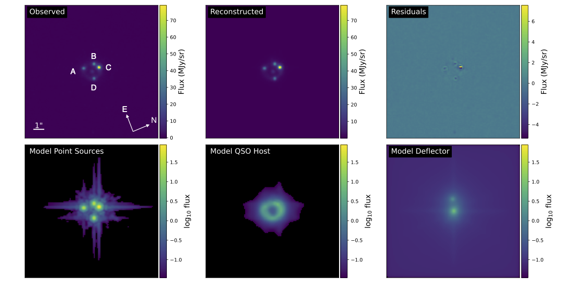
Figure 9: J0405 F560W.

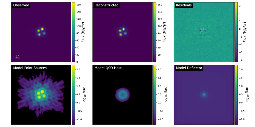
Figure 10: J0405 F1280W.

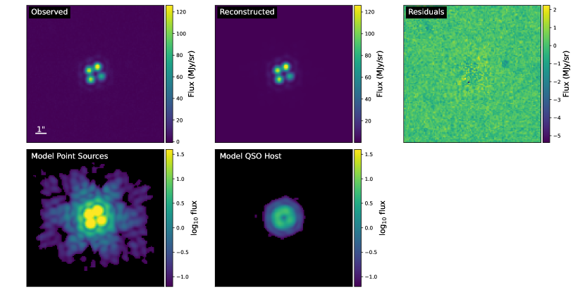
Figure 11: J0405 F1800W.

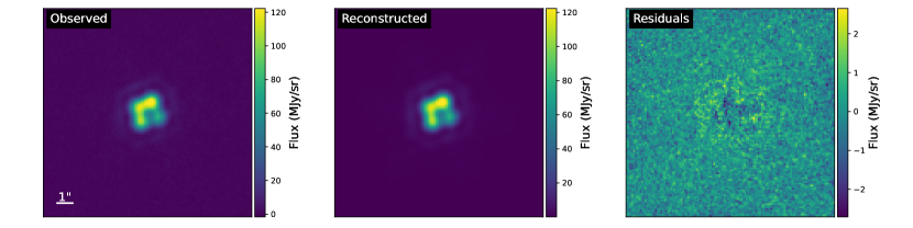
Figure 12: J0405 F2550W.

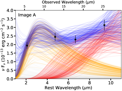
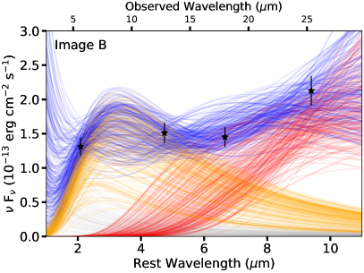
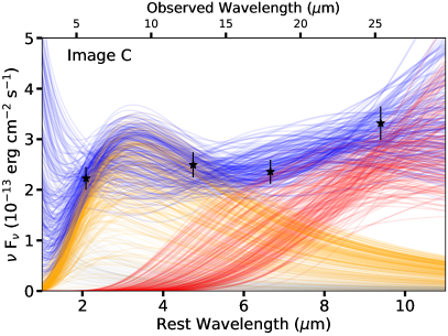
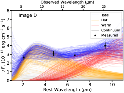
Figure 13: Posterior predictive distributions for the SED fitting for J0405.

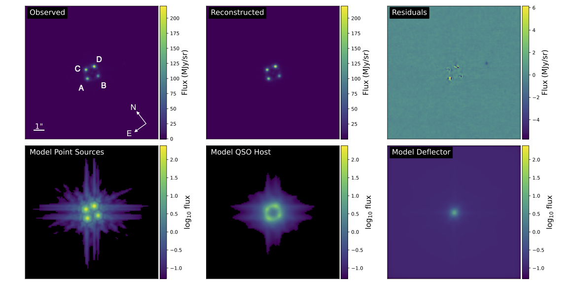
Figure 14: J0607 F560W.

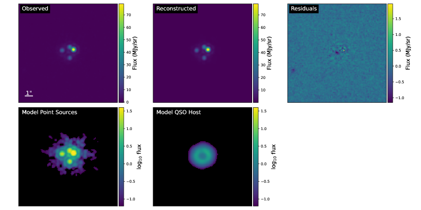
Figure 15: J0607 F1280W.

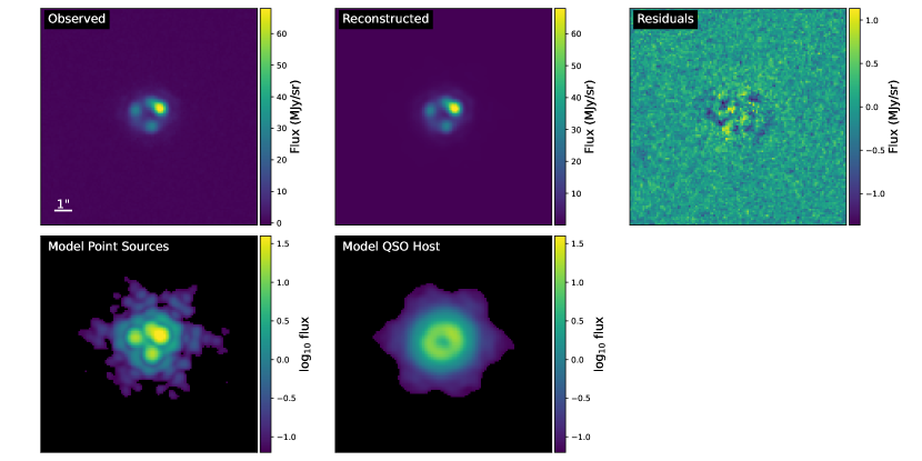
Figure 16: J0607 F1800W.

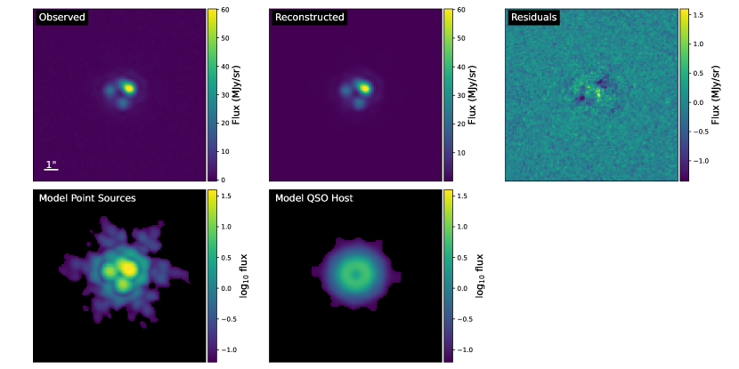
Figure 17: J0607 F2100W.

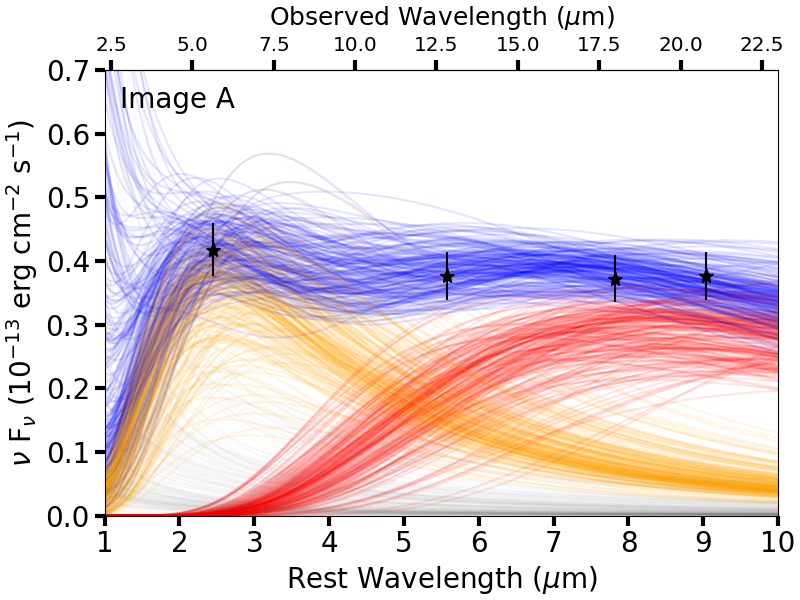
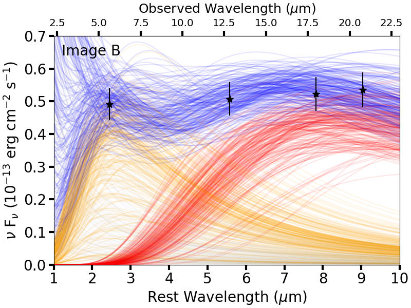
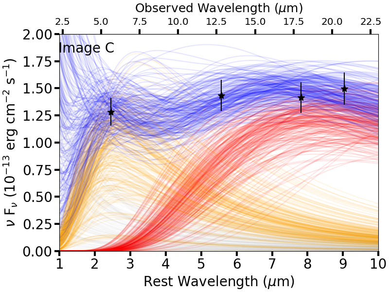
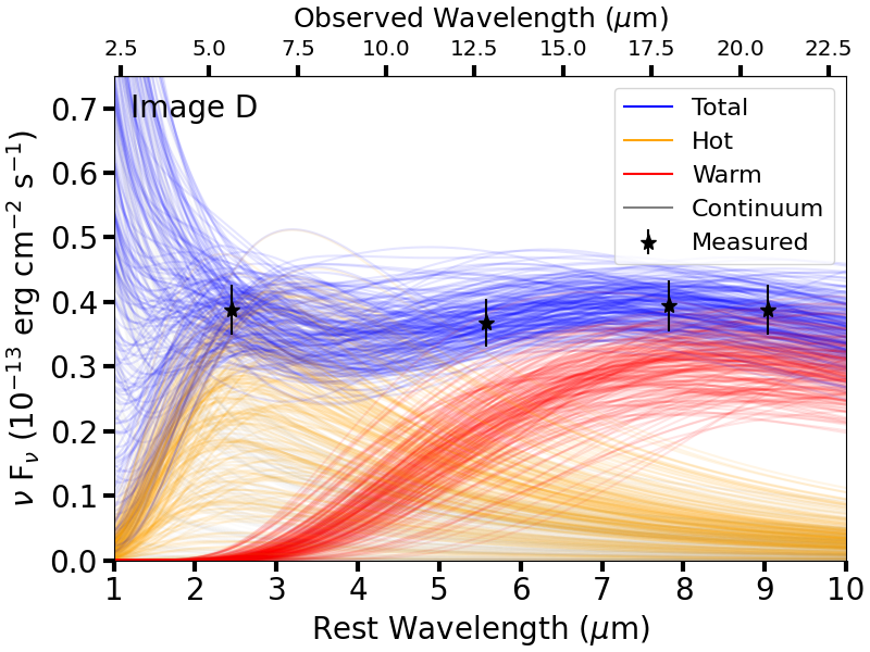
Figure 18: Posterior predictive distributions for the SED fitting for J0607.

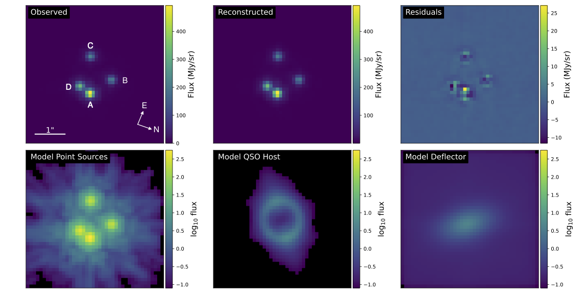
Figure 19: J0608 F560W.

Figure 20: J0608 F1280W.

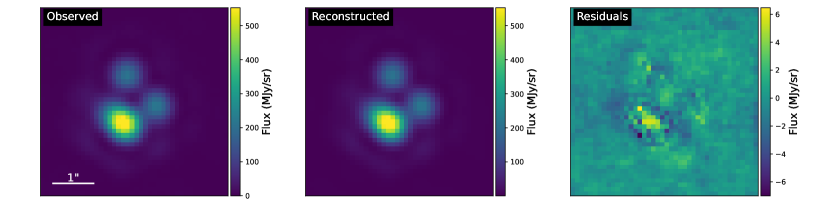
Figure 21: J0608 F1800W.

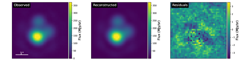
Figure 22: J0608 F2550W.

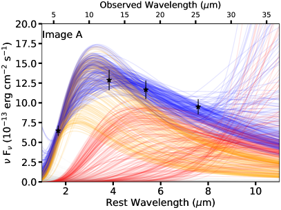
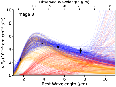
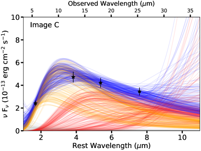
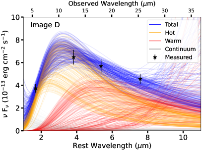
Figure 23: Posterior predictive distributions for the SED fitting for J0608.

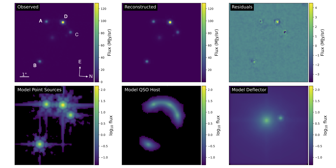
Figure 24: J0659 F560W.

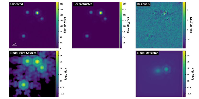
Figure 25: J0659 F1280W.

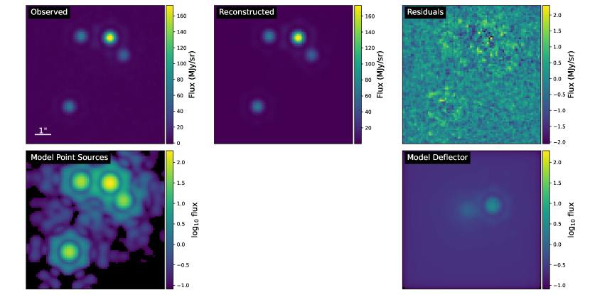
Figure 26: J0659 F1800W.

Figure 27: J0659 F2550W.

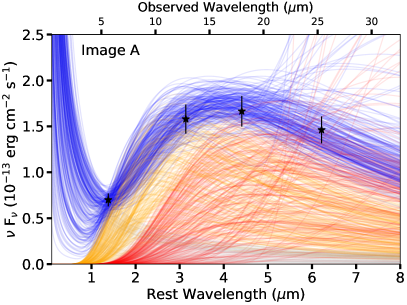
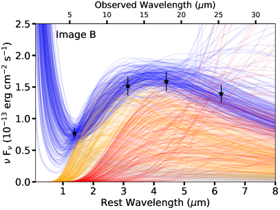
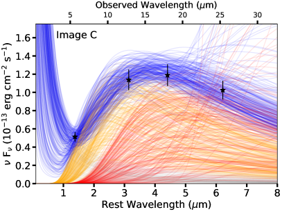
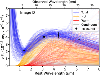
Figure 28: Posterior predictive distributions for the SED fitting for J0659.

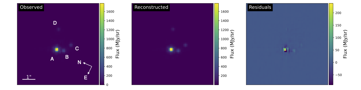
Figure 29: J1042 F560W.

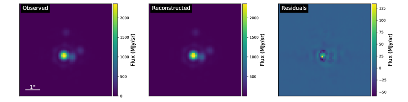
Figure 30: J1042 F1280W.

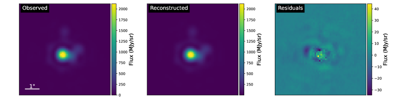
Figure 31: J1042 F1800W.

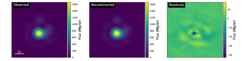
Figure 32: J1042 F2550W.

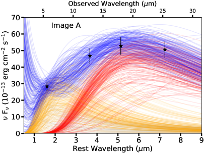
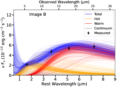
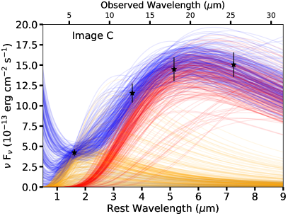
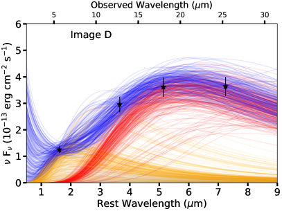
Figure 33: Posterior predictive distributions for the SED fitting for J1042.

Figure 34: J1537 F560W.

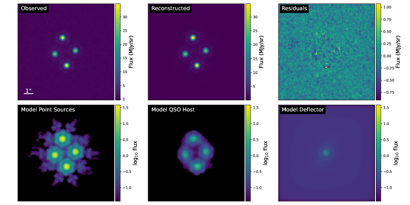
Figure 35: J1537 F1280W.

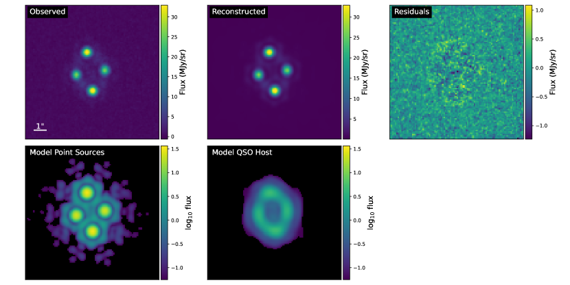
Figure 36: J1537 F1800W.

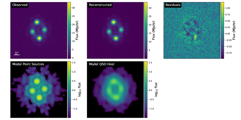
Figure 37: J1537 F2100W.

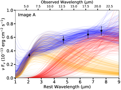
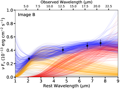
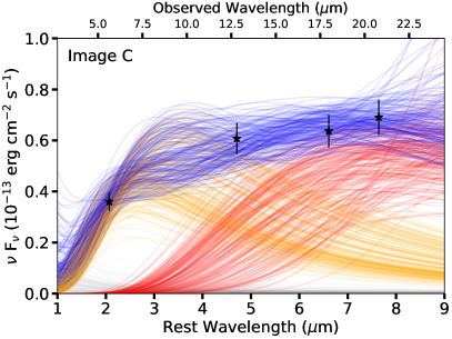
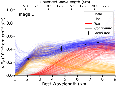
Figure 38: Posterior predictive distributions for the SED fitting for J1537.

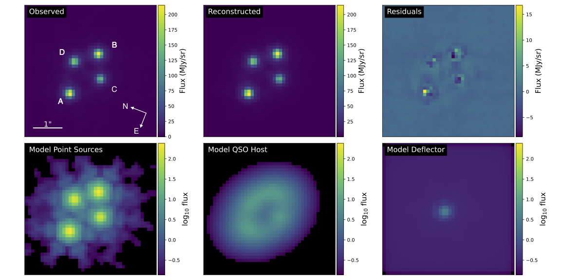
Figure 39: J1606 F560W.

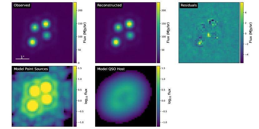
Figure 40: J1606 F1280W.

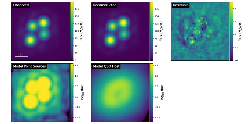
Figure 41: J1606 F1800W.

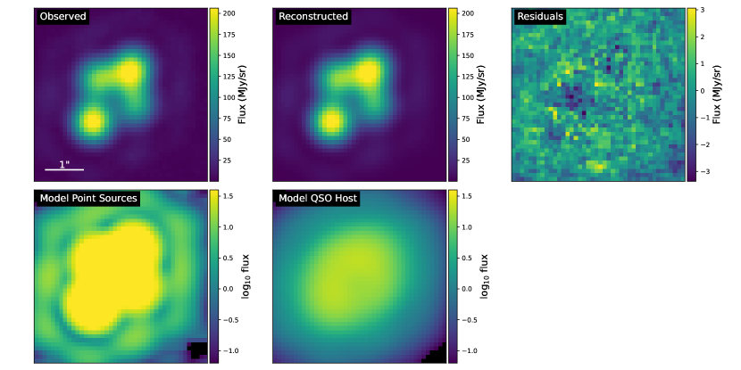
Figure 42: J1606 F2550W.

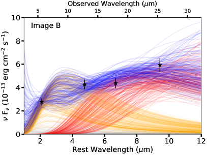
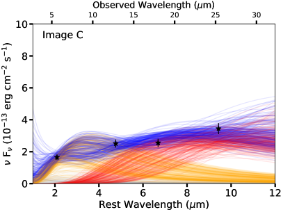
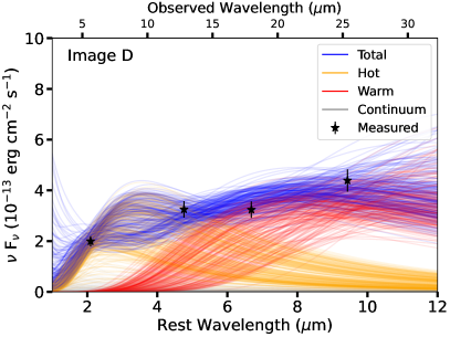
Figure 43: Posterior predictive distributions for the SED fitting for J1606.

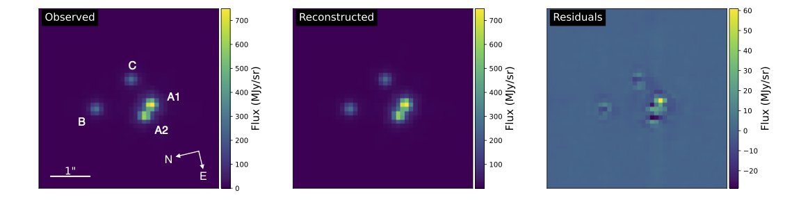
Figure 44: J2026 F560W.

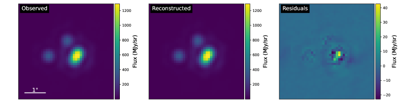
Figure 45: J2026 F1280W.

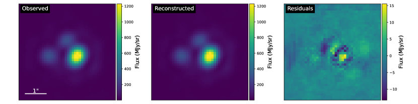
Figure 46: J2026 F1800W.

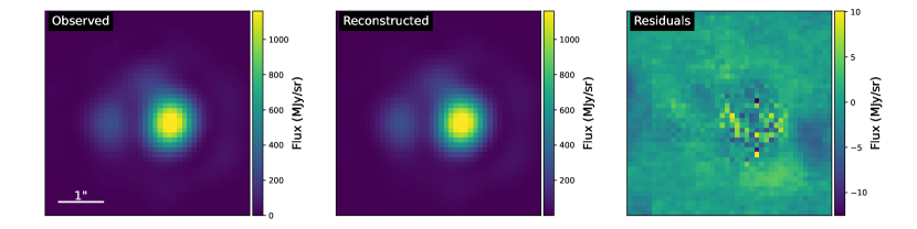
Figure 47: J2026 F2550W.

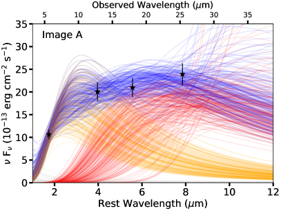
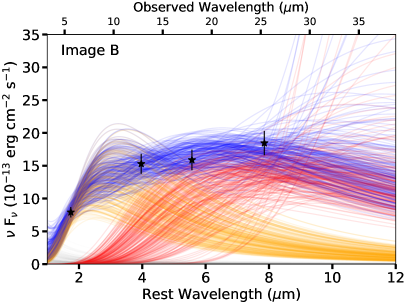
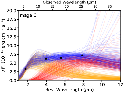
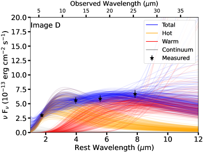
Figure 48: Posterior predictive distributions for the SED fitting for J2026.

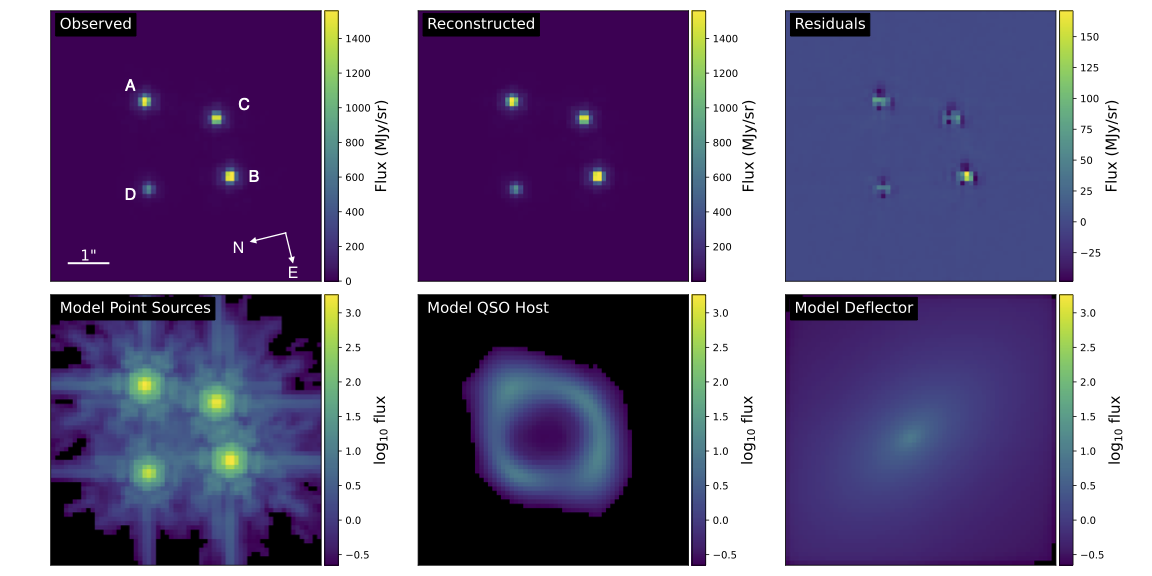
Figure 49: J2038 F560W

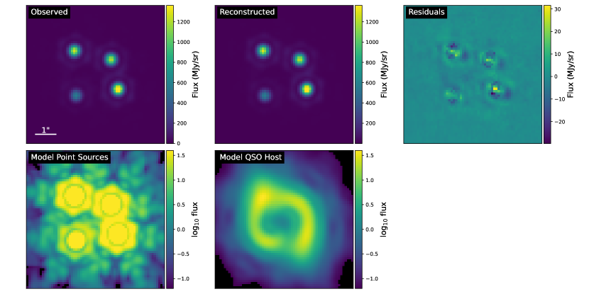
Figure 50: J2038 F1280W

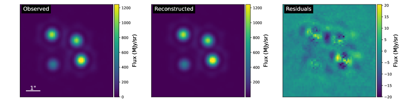
Figure 51: J2038 F1800W

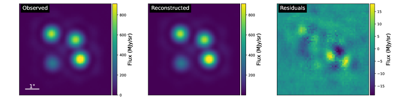
Figure 52: J2038 F2550W

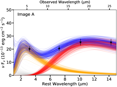
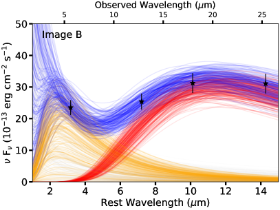
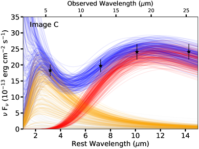
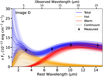
Figure 53: Posterior predictive distributions for the SED fitting for J2038

References

- Agnello et al. (2018) Agnello A., et al., 2018, Monthly Notices of the Royal Astronomical Society, 479, 4345
- Anguita et al. (2018) Anguita T., et al., 2018, Monthly Notices of the Royal Astronomical Society, 480, 5017
- Argyriou et al. (2023) Argyriou I., et al., 2023, The Brighter-Fatter Effect in the JWST MIRI Si:As IBC detectors I. Observations, impact on science, and modelling, doi:10.48550/arXiv.2303.13517, https://ui.adsabs.harvard.edu/abs/2023arXiv230313517A
- Banik et al. (2018) Banik N., Bertone G., Bovy J., Bozorgnia N., 2018, J. Cosmology Astropart. Phys., 2018, 061
- Banik et al. (2021a) Banik N., Bovy J., Bertone G., Erkal D., de Boer T. J. L., 2021a, Monthly Notices of the Royal Astronomical Society, 502, 2364
- Banik et al. (2021b) Banik N., Bovy J., Bertone G., Erkal D., de Boer T. J. L., 2021b, J. Cosmology Astropart. Phys., 2021, 043
- Bechtol et al. (2019) Bechtol K., et al., 2019, BAAS, 51, 207
- Benson (2012) Benson A. J., 2012, doi:10.1016/j.newast.2011.07.004, 17, 175
- Benson & Du (2022) Benson A. J., Du X., 2022, MNRAS, 517, 1398
- Birrer & Amara (2018) Birrer S., Amara A., 2018, Physics of the Dark Universe, 22, 189
- Birrer et al. (2021) Birrer S., et al., 2021, The Journal of Open Source Software, 6, 3283
- Boddy et al. (2022) Boddy K. K., et al., 2022, Journal of High Energy Astrophysics, 35, 112
- Bode et al. (2001) Bode P., Ostriker J. P., Turok N., 2001, The Astrophysical Journal, 556, 93
- Bonaca et al. (2019) Bonaca A., Hogg D. W., Price-Whelan A. M., Conroy C., 2019, ApJ, 880, 38
- Bose et al. (2016) Bose S., Hellwing W. A., Frenk C. S., Jenkins A., Lovell M. R., Helly J. C., Li B., 2016, Monthly Notices of the Royal Astronomical Society, 455, 318
- Bovy et al. (2017) Bovy J., Erkal D., Sanders J. L., 2017, MNRAS, 466, 628
- Buckley & Peter (2018) Buckley M. R., Peter A. H. G., 2018, Physics Reports, 761, 1
- Bullock & Boylan-Kolchin (2017) Bullock J. S., Boylan-Kolchin M., 2017, Annual Review of Astronomy and Astrophysics, 55, 343
- Burtscher et al. (2013) Burtscher L., et al., 2013, Astronomy and Astrophysics, 558, A149
- Cohen et al. (2024) Cohen J. S., Fassnacht C. D., O’Riordan C. M., Vegetti S., 2024, arXiv e-prints, p. arXiv:2403.08895
- Cooley et al. (2022) Cooley J., et al., 2022, arXiv e-prints, p. arXiv:2209.07426
- Dalal & Kochanek (2002) Dalal N., Kochanek C. S., 2002, The Astrophysical Journal, 572, 25
- Dekker et al. (2022) Dekker A., Ando S., Correa C. A., Ng K. C. Y., 2022, Physical Review D, 106, 123026
- Delchambre et al. (2019) Delchambre L., et al., 2019, Astronomy and Astrophysics, 622, A165
- Despali et al. (2016) Despali G., Giocoli C., Angulo R. E., Tormen G., Sheth R. K., Baso G., Moscardini L., 2016, MNRAS, 456, 2486
- Diemer & Joyce (2019) Diemer B., Joyce M., 2019, ApJ, 871, 168
- Dike et al. (2023) Dike V., Gilman D., Treu T., 2023, Monthly Notices of the Royal Astronomical Society, 522, 5434
- Drlica-Wagner et al. (2019) Drlica-Wagner A., et al., 2019, arXiv e-prints, p. arXiv:1902.01055
- Du et al. (2024) Du X., et al., 2024, arXiv e-prints, p. arXiv:2403.09597
- Errani & Navarro (2021) Errani R., Navarro J. F., 2021, MNRAS, 505, 18
- Fiacconi et al. (2016) Fiacconi D., Madau P., Potter D., Stadel J., 2016, The Astrophysical Journal, 824, 144
- Foreman-Mackey et al. (2013) Foreman-Mackey D., Hogg D. W., Lang D., Goodman J., 2013, Publications of the Astronomical Society of the Pacific, 125, 306
- Gao et al. (2012) Gao L., Navarro J. F., Frenk C. S., Jenkins A., Springel V., White S. D. M., 2012, Monthly Notices of the Royal Astronomical Society, 425, 2169
- García-Bernete et al. (2022) García-Bernete I., et al., 2022, A high angular resolution view of the PAH emission in Seyfert galaxies using JWST/MRS data, doi:10.1051/0004-6361/202244806, https://arxiv.org/abs/2208.11620v2
- Gilman et al. (2019) Gilman D., Birrer S., Treu T., Nierenberg A., Benson A., 2019, Monthly Notices of the Royal Astronomical Society, 487, 5721
- Gilman et al. (2020a) Gilman D., Birrer S., Nierenberg A., Treu T., Du X., Benson A., 2020a, Monthly Notices of the Royal Astronomical Society, 491, 6077
- Gilman et al. (2020b) Gilman D., Du X., Benson A., Birrer S., Nierenberg A., Treu T., 2020b, Monthly Notices of the Royal Astronomical Society, 492, L12
- Gilman et al. (2021) Gilman D., Bovy J., Treu T., Nierenberg A., Birrer S., Benson A., Sameie O., 2021, Monthly Notices of the Royal Astronomical Society, 507, 2432
- Gilman et al. (2022) Gilman D., Benson A., Bovy J., Birrer S., Treu T., Nierenberg A., 2022, Monthly Notices of the Royal Astronomical Society, 512, 3163
- Gilman et al. (2023) Gilman D., Zhong Y.-M., Bovy J., 2023, Physical Review D, 107, 103008
- Gilman et al. (2024) Gilman D., Birrer S., Nierenberg A., Oh M. S. H., 2024, arXiv e-prints, p. arXiv:2403.03253
- Glikman et al. (2023) Glikman E., et al., 2023, ApJ, 943, 25
- Gordon et al. (2022) Gordon K. D., et al., 2022, The Astronomical Journal, 163, 267
- Griffen et al. (2016) Griffen B. F., Ji A. P., Dooley G. A., Gómez F. A., Vogelsberger M., O’Shea B. W., Frebel A., 2016, The Astrophysical Journal, 818, 10
- Gáspár et al. (2021) Gáspár A., et al., 2021, Publications of the Astronomical Society of the Pacific, 133, 014504
- Hao et al. (2006) Hao C. N., Mao S., Deng Z. G., Xia X. Y., Wu H., 2006, Monthly Notices of the Royal Astronomical Society, 370, 1339
- He et al. (2024) He Q., et al., 2024, arXiv e-prints, p. arXiv:2403.16253
- Hernán-Caballero et al. (2016) Hernán-Caballero A., Hatziminaoglou E., Alonso-Herrero A., Mateos S., 2016, Monthly Notices of the Royal Astronomical Society, 463, 2064
- Hinshaw et al. (2013) Hinshaw G., et al., 2013, ApJS, 208, 19
- Hsueh et al. (2020) Hsueh J. W., Enzi W., Vegetti S., Auger M. W., Fassnacht C. D., Despali G., Koopmans L. V. E., McKean J. P., 2020, Monthly Notices of the Royal Astronomical Society, 492, 3047
- Iršič et al. (2017) Iršič V., et al., 2017, Phys. Rev. D, 96, 023522
- Jensen et al. (2017) Jensen J. J., et al., 2017, MNRAS, 470, 3071
- Jiang et al. (2015) Jiang L., Cole S., Sawala T., Frenk C. S., 2015, MNRAS, 448, 1674
- Koekemoer et al. (2007) Koekemoer A. M., et al., 2007, The Astrophysical Journal Supplement Series, 172, 196
- Lagattuta et al. (2010) Lagattuta D. J., et al., 2010, The Astrophysical Journal, 716, 1579
- Laroche et al. (2022) Laroche A., Gilman D., Li X., Bovy J., Du X., 2022, Monthly Notices of the Royal Astronomical Society, 517, 1867
- Lazar et al. (2021) Lazar A., Bullock J. S., Boylan-Kolchin M., Feldmann R., Çatmabacak O., Moustakas L., 2021, MNRAS, 502, 6064
- Leftley et al. (2019) Leftley J. H., Hönig S. F., Asmus D., Tristram K. R. W., Gandhi P., Kishimoto M., Venanzi M., Williamson D. J., 2019, The Astrophysical Journal, 886, 55
- Lemon et al. (2018) Lemon C. A., Auger M. W., McMahon R. G., Ostrovski F., 2018, MNRAS, 479, 5060
- Lemon et al. (2023) Lemon C., et al., 2023, MNRAS, 520, 3305
- Lintusaari et al. (2017) Lintusaari J., Gutmann M. U., Dutta R., Kaski S., Corander J., 2017, Systematic Biology, 66, e66
- Lovell (2020) Lovell M. R., 2020, ApJ, 897, 147
- Lovell et al. (2014) Lovell M. R., Frenk C. S., Eke V. R., Jenkins A., Gao L., Theuns T., 2014, MNRAS, 439, 300
- Ludlow et al. (2014) Ludlow A. D., Navarro J. F., Angulo R. E., Boylan-Kolchin M., Springel V., Frenk C., White S. D. M., 2014, MNRAS, 441, 378
- Ludlow et al. (2016) Ludlow A. D., Bose S., Angulo R. E., Wang L., Hellwing W. A., Navarro J. F., Cole S., Frenk C. S., 2016, Monthly Notices of the Royal Astronomical Society, 460, 1214
- Mao & Schneider (1998) Mao S., Schneider P., 1998, Monthly Notices of the Royal Astronomical Society, 295, 587
- Marin et al. (2011) Marin J.-M., Pudlo P., Robert C. P., Ryder R., 2011, arXiv e-prints, p. arXiv:1101.0955
- Meneghetti et al. (2020) Meneghetti M., et al., 2020, Science, 369, 1347
- Minor et al. (2021) Minor Q., Gad-Nasr S., Kaplinghat M., Vegetti S., 2021, Monthly Notices of the Royal Astronomical Society, 507, 1662
- Morgan et al. (2004) Morgan N. D., Caldwell J. A. R., Schechter P. L., Dressler A., Egami E., Rix H.-W., 2004, AJ, 127, 2617
- Müller-Sánchez et al. (2011) Müller-Sánchez F., Prieto M. A., Hicks E. K. S., Vives-Arias H., Davies R. I., Malkan M., Tacconi L. J., Genzel R., 2011, The Astrophysical Journal, 739, 69
- Nadler et al. (2020) Nadler E. O., et al., 2020, The Astrophysical Journal, 893, 48
- Nadler et al. (2021a) Nadler E. O., et al., 2021a, Physical Review Letters, 126, 091101
- Nadler et al. (2021b) Nadler E. O., Birrer S., Gilman D., Wechsler R. H., Du X., Benson A., Nierenberg A. M., Treu T., 2021b, The Astrophysical Journal, 917, 7
- Navarro et al. (1997) Navarro J. F., Frenk C. S., White S. D. M., 1997, The Astrophysical Journal, 490, 493
- Newton et al. (2021) Newton O., et al., 2021, J. Cosmology Astropart. Phys., 2021, 062
- Nierenberg et al. (2014) Nierenberg A. M., Treu T., Wright S. A., Fassnacht C. D., Auger M. W., 2014, Monthly Notices of the Royal Astronomical Society, 442, 2434
- Nierenberg et al. (2016) Nierenberg A. M., Treu T., Menci N., Lu Y., Torrey P., Vogelsberger M., 2016, MNRAS, 462, 4473
- Nierenberg et al. (2017) Nierenberg A. M., et al., 2017, Monthly Notices of the Royal Astronomical Society, 471, 2224
- Nierenberg et al. (2020) Nierenberg A. M., et al., 2020, Monthly Notices of the Royal Astronomical Society, 492, 5314
- Nierenberg et al. (2023) Nierenberg A. M., et al., 2023, arXiv e-prints, p. arXiv:2309.10101
- Oh et al. (2024) Oh M. S. H., Nierenberg A., Gilman D., Birrer S., 2024, arXiv e-prints, p. arXiv:2404.17124
- Perrin et al. (2012) Perrin M. D., Soummer R., Elliott E. M., Lallo M. D., Sivaramakrishnan A., 2012, in Space Telescopes and Instrumentation 2012: Optical, Infrared, and Millimeter Wave. SPIE, pp 1193–1203, doi:10.1117/12.925230, https://www.spiedigitallibrary.org/conference-proceedings-of-spie/8442/84423D/Simulating-point-spread-functions-for-the-James-Webb-Space-Telescope/10.1117/12.925230.full
- Perrin et al. (2014) Perrin M. D., Sivaramakrishnan A., Lajoie C.-P., Elliott E., Pueyo L., Ravindranath S., Albert L., 2014, in Space Telescopes and Instrumentation 2014: Optical, Infrared, and Millimeter Wave. SPIE, pp 1174–1184, doi:10.1117/12.2056689, https://www.spiedigitallibrary.org/conference-proceedings-of-spie/9143/91433X/Updated-point-spread-function-simulations-for-JWST-with-WebbPSF/10.1117/12.2056689.full
- Planck Collaboration, (2020) Planck Collaboration, 2020, Astronomy & Astrophysics, 641, A6
- Powell et al. (2023) Powell D. M., Vegetti S., McKean J. P., White S. D. M., Ferreira E. G. M., May S., Spingola C., 2023, Monthly Notices of the Royal Astronomical Society, 524, L84
- Rubin (1984) Rubin D. B., 1984, The Annals of Statistics, 12, 1151
- Schmidt et al. (2023) Schmidt T., et al., 2023, Monthly Notices of the Royal Astronomical Society, 518, 1260
- Schneider et al. (2012) Schneider A., Smith R. E., Macciò A. V., Moore B., 2012, Monthly Notices of the Royal Astronomical Society, 424, 684
- Schneider et al. (2013) Schneider A., Smith R. E., Reed D., 2013, MNRAS, 433, 1573
- Shajib et al. (2019) Shajib A. J., et al., 2019, Monthly Notices of the Royal Astronomical Society, 483, 5649
- Sheth et al. (2001) Sheth R. K., Mo H. J., Tormen G., 2001, MNRAS, 323, 1
- Sluse et al. (2013) Sluse D., Kishimoto M., Anguita T., Wucknitz O., Wambsganss J., 2013, Astronomy and Astrophysics, 553, A53
- Springel et al. (2008) Springel V., et al., 2008, MNRAS, 391, 1685
- Stacey & McKean (2018) Stacey H. R., McKean J. P., 2018, MNRAS, 481, L40
- Stacey et al. (2020) Stacey H. R., Lafontaine A., McKean J. P., 2020, MNRAS, 493, 5290
- Stacey et al. (2024) Stacey H. R., Powell D. M., Vegetti S., McKean J. P., Fassnacht C. D., Wen D., O’Riordan C. M., 2024, arXiv e-prints, p. arXiv:2403.04850
- Stern et al. (2021) Stern D., et al., 2021, ApJ, 921, 42
- Stücker et al. (2023) Stücker J., Ogiya G., Angulo R. E., Aguirre-Santaella A., Sánchez-Conde M. A., 2023, MNRAS, 521, 4432
- Sérsic (1963) Sérsic J. L., 1963, Boletin de la Asociacion Argentina de Astronomia La Plata Argentina, 6, 41
- Tegmark et al. (2004) Tegmark M., et al., 2004, Phys. Rev. D, 69, 103501
- Tessore & Metcalf (2015) Tessore N., Metcalf R. B., 2015, Astronomy & Astrophysics, 580, A79
- Tollerud et al. (2008) Tollerud E. J., Bullock J. S., Strigari L. E., Willman B., 2008, ApJ, 688, 277
- Tommasin et al. (2010) Tommasin S., Spinoglio L., Malkan M. A., Fazio G., 2010, ApJ, 709, 1257
- Treu (2010) Treu T., 2010, ARA&A, 48, 87
- Vegetti et al. (2018) Vegetti S., Despali G., Lovell M. R., Enzi W., 2018, Monthly Notices of the Royal Astronomical Society, 481, 3661
- Vegetti et al. (2023) Vegetti S., et al., 2023, arXiv e-prints, p. arXiv:2306.11781
- Viel et al. (2013) Viel M., Becker G. D., Bolton J. S., Haehnelt M. G., 2013, Phys. Rev. D, 88, 043502
- Villasenor et al. (2023) Villasenor B., Robertson B., Madau P., Schneider E., 2023, Phys. Rev. D, 108, 023502
- Vogel & Abazajian (2023) Vogel C. M., Abazajian K. N., 2023, Phys. Rev. D, 108, 043520
- Wechsler et al. (2002) Wechsler R. H., Bullock J. S., Primack J. R., Kravtsov A. V., Dekel A., 2002, ApJ, 568, 52
- Weinberg et al. (2015) Weinberg D. H., Bullock J. S., Governato F., Kuzio de Naray R., Peter A. H. G., 2015, Proceedings of the National Academy of Science, 112, 12249
- White & Frenk (1991) White S. D. M., Frenk C. S., 1991, The Astrophysical Journal, 379, 52
- White & Rees (1978) White S. D. M., Rees M. J., 1978, Monthly Notices of the Royal Astronomical Society, 183, 341
- Wright et al. (2023) Wright G. S., et al., 2023, Publications of the Astronomical Society of the Pacific, 135, 048003
- Xu et al. (2015) Xu D., Sluse D., Gao L., Wang J., Frenk C., Mao S., Schneider P., Springel V., 2015, MNRAS, 447, 3189
- Yang & Yu (2021) Yang D., Yu H.-B., 2021, Phys. Rev. D, 104, 103031
- Yang et al. (2020) Yang S., Du X., Benson A. J., Pullen A. R., Peter A. H. G., 2020, MNRAS, 498, 3902
- Zelko et al. (2022) Zelko I. A., Treu T., Abazajian K. N., Gilman D., Benson A. J., Birrer S., Nierenberg A. M., Kusenko A., 2022, Physical Review Letters, 129, 191301
- de Blok et al. (2008) de Blok W. J. G., Walter F., Brinks E., Trachternach C., Oh S. H., Kennicutt R. C. J., 2008, AJ, 136, 2648