A probabilistic estimation of remaining useful life from censored time-to-event data

Abstract

Predicting the remaining useful life (RUL) of ball bearings plays an important role in predictive maintenance. A common definition of the RUL is the time until a bearing is no longer functional, which we denote as an event, and many data-driven methods have been proposed to predict the RUL. However, few studies have addressed the problem of censored data, where this event of interest is not observed, and simply ignoring these observations can lead to an overestimation of the failure risk. In this paper, we propose a probabilistic estimation of RUL using survival analysis that supports censored data. First, we analyze sensor readings from ball bearings in the frequency domain and annotate when a bearing starts to deteriorate by calculating the Kullback-Leibler (KL) divergence between the probability density function (PDF) of the current process and a reference PDF. Second, we train several survival models on the annotated bearing dataset, capable of predicting the RUL over a finite time horizon using the survival function. This function is guaranteed to be strictly monotonically decreasing and is an intuitive estimation of the remaining lifetime. We demonstrate our approach in the XJTU-SY dataset using cross-validation and find that Random Survival Forests consistently outperforms both non-neural networks and neural networks in terms of the mean absolute error (MAE). Our work encourages the inclusion of censored data in predictive maintenance models and highlights the unique advantages that survival analysis offers when it comes to probabilistic RUL estimation and early fault detection.

1 Introduction

Rolling bearings have extensive applications in various rotating machines, such as pumps, electric motors, wind turbines, and vehicles, but are also the most susceptible component in many mechanical systems. Therefore, for decades, engineers and scientists have focused on detecting faults in these bearings so that maintenance and repairs can be performed before a failure occurs. Faults and defects are often induced by contamination wear, poor lubrication, and improper mounting, among others [9, 34, 31, 14]. However, accurately identifying the presence of a fault can be challenging in practical scenarios, particularly when the fault is in its early stages (incipient stage) and the signal-to-noise ratio of the monitored signal is low.

A defect primarily induces mechanical vibrations that can be detected by an accelerometer or microphone and used to determine whether a fault is present or not. Traditionally, mechanical engineers have used model-based methods, which are based solely on threshold values of different signals (data) at predetermined fault frequencies to detect bearing faults. Therefore, these models can only describe the signal characteristics of a few specific fault types, but real-world bearing faults are often more complex. Alternatively, many researchers have adopted a data-driven approach using machine learning (ML) and deep learning (DL) [19, 6, 7, 40]. This approach stands in contrast to the conventional model-based methods described above, as it offers a more sophisticated, less error-prone, and more precise means of assessing the health of a bearing [61, 37].

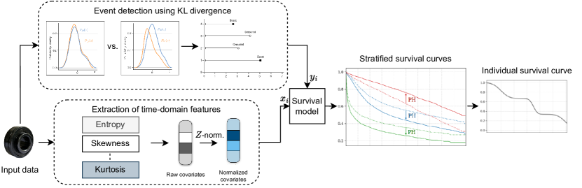
Figure 1: Outline of proposed solution. The raw data are used for event detection in the frequency domain (top) and for feature extraction in the time domain (bottom) before training a survival model. Illustrations in part from [43].

An important metric in bearing diagnostics is the remaining useful life (RUL). The RUL is defined as the time interval between the current inspection time and a future point in time at which the bearing will stop working. The RUL is considered an important indicator of a bearing’s health and can be used to detect faults before they lead to failures [25, 76, 1, 62, 65, 70, 71]. Accurately estimating the RUL can help engineers plan for maintenance in advance and thereby enhance the overall reliability and safety of the machinery.

However, despite numerous advances in model development and increases in predictive performance, several challenges still exist in RUL estimation: (1) In real applications, there is generally a high level of uncertainty at the prediction stage on unseen data, but many methods do not model the predictive uncertainty at all and simply estimate the remaining useful life as a point prediction [18]. In particular, deep learning models based on the maximum likelihood estimate (MLE) do not allow for uncertainty representation in regression settings, and deep learning classification models often give normalized score vectors, which do not necessarily capture model uncertainty [21]. (2) Bearing failure is a rare event, in the sense that the number of data samples where the bearing operates without problems far outweighs the number of samples with failure indications [18]. This leads to data sparsity, which is a particular problem for MLE-based approaches [21]. (3) Censored or incomplete observations (where the event of interest is not observed) is a prevalent phenomenon given the rarity of failures or breakdowns [18], yet, few studies have so far attempted to model or addressed the consequences of censoring [68, 67, 27]. Alternatively, we can choose to simply ignore the censored observations and analyze only samples where we know the true outcome. However, this leads to a loss of efficiency, as the sample size would be considerably smaller, and introduces an estimation bias. If we want to accurately estimate when a bearing is likely to break down based on historical data and current sensor data, we should include information from censored data samples in the model.

In this paper, we propose an interpretable event detection algorithm that can detect significant discrepancies in the frequencies of a bearing, indicating a potential future mechanical failure. We use this algorithm as an oracle to label a ball bearing dataset for subsequent RUL estimation. Specifically, for event detection, we compare the Kullback-Leibler (KL) divergence between the magnitude spectrum of the current signal and the magnitude spectrum of a reference signal. This divergence becomes significant as the bearing starts to deteriorate. Thus, it is a useful indicator of the bearing’s health state. For RUL estimation, we propose a covariate-based survival analysis model that (1) provides RUL curves that are guaranteed to be monotonically decreasing along time, (2) offers a probabilistic estimation of the RUL instead of just a point estimate, and (3) naturally supports censored observations to not overestimate the risk of an event. In this context, the covariates (features) are extracted from the time domain and include information such as skewness, kurtosis, and entropy. For our empirical analyses, we adopt XJTU-SY dataset [62], which consists of five ball bearings per operating condition (C1-C3), and show that our method can reliably detect bearing faults early and also accurately estimate the RUL as the time to predictive maintenance. Unlike many state-of-the-art works on RUL prediction [71, 65], our method provides a probabilistic estimate of the RUL in minutes that can assist maintenance personnel to make informed decisions regarding whether to inspect or replace a bearing.

Overall, our work is an extension of [39], and offers several new improvements: we evaluate our method under various operating conditions, we stratify the covariates to assess any statistical differences in survival time between groups of bearings, and we offer a probabilistic estimate of the RUL. We achieve the latter by predicting a survival curve for each bearing and taking the time of the median probability (0.5) as the time to event. Moreover, we adopt a Bayesian Neural Network (BNN), since such models have shown promise in performance prognostics [64], and can provide uncertainty quantification through percentage credible intervals (CrIs) around the survival curve [47]. Figure 1 shows our proposed solution for early event detection and RUL estimation in ball bearings. In summary, our contributions are as follows:

• We propose a novel event detection algorithm to label a ball bearing dataset based on the KL divergence.

• We present a method that provides a probabilistic estimate of the RUL, which can guide decision-making on whether bearings need further inspection or should be replaced.

• We demonstrate the effectiveness of our approach by measuring its prediction and calibration performance using cross-validation on the XJTU-SY dataset.

All experiments are made with Python and are fully reproducible. The source code and data will be publicly available at:
https://github.com/thecml/rulsurv

2 Related work

Event detection focuses on detecting when a bearing is likely to fail and understanding the relationship between bearing faults and measurable signals. This is usually done by analyzing readings from a bearing sensor, which includes vibrations and acoustic noise measurements, and then establishing a threshold value of each input reading. On the other hand, RUL estimation aims to proactively predict the remaining time that a bearing can operate before it fails. This is typically done by adopting a data-driven approach that learns patterns in historical data to estimate the remaining useful life of new and unseen bearings. In this section, we provide a brief overview of the latest research in these two domains, their limitations, and motivate our approach.

2.1 Event detection

Numerous algorithms have been proposed to detect faults in bearings. These include artificial neural networks (ANNs) [60], Principal Component Analysis (PCA) [17], K-Nearest Neighbors (KNN) [2], Convolutional Neural Networks (CNNs) [11], Deep Autoencoders [71], Recurrent Neural Networks (RNNs) [53] and attention-based methods [57]. Although DL approaches have outperformed classical approaches in terms of predictive accuracy, they usually require large amounts of data and inherently lack interpretability: it is practically impossible for humans to trace the precise mapping from input data to prediction in a neural network [24, 59], and thus specific interpretation methods have to be used [42]. However, one of the classical approaches that remains relevant is the KL divergence. It is a distance-based metric that measures the difference (entropy) between two probability distributions [35]. It can detect anomalous events by comparing the probability density function (PDF) of the current process with a reference probability density function. The KL divergence has seen widespread adoption as a health degradation indicator [73, 15, 48, 69], and offers a simple and interpretable indication for when a bearing is approaching its end of life.

2.2 RUL prediction

Research practitioners and engineers often predict RUL by adopting a model-based or a data-driven approach: model-based methods involve developing mathematical or physical models based on historical data to determine trends in the health status of a component [11]. On the other hand, a data-driven approach develops a model on historical data and then determines patterns in unseen data [11], which encompasses ML methods [18]. Similarly, despite their need for large amounts of historical data in model development, data-driven methods are less complex, more precise, and more applicable in real life than model-based methods [61, 37]. The availability of large data streams and newer technologies to reliably record sensor readings has also fueled the popularity of data-driven methods, and notable works also rely on a deep learning architecture.

[67] presented a data-driven model to assess machine degradation and directly addresses the problem of censored data by training a relevance vector machine (RVM) using survival analysis. Survival analysis is a form of regression modeling that studies the time to an event, which can be partially observed (that is, censored) and has found important use in applications in multiple domains, such as healthcare informatics [77, 33], econometrics [56], and in engineering, including predictive maintenance [67, 68, 27, 63]. The main idea proposed by [67] revolves around predicting the survival probability, indicating when an individual machine component is likely to fail as a function of the measurement points. They provide an intuitive and probabilistic explanation of a bearing’s anticipated failure rate, highlighting distinct declines leading to the eventual failure with quantitative measurements. However, their study does not compare the proposed method to others, and the result is based only on survival curves by the Kaplan-Meier (KM) estimator [32]. Although mathematically robust, nonparametric tests are often hard to interpret and KM-based survival analysis uses only a single binary predictor, while Cox regression can use both continuous predictors, binary predictors, and nonparametric tests [13].

[25] proposed a recurrent neural network to predict the health of a bearing. This is done by first recording similarity measures between the current data reading and data at an initial operation point as a feature from zero to one and then training the RNN to map this feature value to some degradation percentage. They trained their model, RNN-HI, on the XJTU-SY dataset [62], and demonstrated a significant improvement in the prediction of RUL compared to using self-organizing maps (SOM) [28].

[10] proposed a Cox model that can predict the time between failures in automobiles. They used an auto-encoder for data representation, a Cox proportional hazard model for censored data estimation, and a long-short-term memory (LSTM) network to train the prediction model. However, the Cox model is used only to label the censored data, and the prediction problem is then framed as a traditional regression problem without paying attention to the censoring. It also remains unclear how the Cox model was evaluated.

[65] proposed a Cox feature fusion model to predict RUL in bearings, including several steps. First, they train a feature fusion algorithm (KPCA) that fuses multiple feature indicators based on sensor readings. Second, they performed a Pearson’s correlation analysis to obtain a correlation matrix. Third, they trained an LSTM model to produce multidimensional covariates based on this feature matrix, and finally, its output is forwarded to a Cox model to obtain the probability of failure for each bearing. They provided bearing-specific amplitude readings and predictions as a function of sampling points, showing promise, but they did not offer any evaluation of predictive accuracy. The proposed model was evaluated only on two actual bearings from the Intelligent System Maintenance dataset [49], but the authors did not provide quantitative performance measurements, and it remains unclear when or how they established the event of interest.

[71] proposed a novel health indicator framework for automatic RUL prediction based on a multihead attention architecture, combining information from damaged and healthy bearings to improve prediction accuracy. Their method achieves a good prediction error compared to other works, but the estimated RUL is not strictly monotonically decreasing, and the authors make the assumption of a linear correlation between the RUL and a bearing’s lifetime. Assuming a linear RUL oversimplifies the bearing degradation process, as the relationship between the RUL and the number of life cycles is often nonlinear [34, Ch. 2]. Bearings may not degrade at a constant speed, however, as their health can depend on various factors, such as the operating condition, temperature, maintenance, or other external factors [75].

3 Fundamentals

3.1 Elements of rolling bearings

Mechanical bearings are used to carry axial or radial loads during rotational or oscillating motion with minimal friction. During the operation of a bearing, the rolling elements in motion are separated by a lubricant film. This is to avoid contact with the surface asperity during motion and to distribute the applied axial or radial load across the load zone beneath the rolling elements. Bearing health depends on a wide range of factors, such as operating conditions, temperature, and maintenance level, among others [75]. Therefore, it is challenging to predict the actual end of life of an individual bearing. To establish a benchmark for bearing life expectancy, a standard industry measurement is the $L_{10}$ bearing lifetime. Specifically, the $L_{10}$ indicates the number of hours that a group of identical bearings, running at a constant speed, will last before a 10% of them fail [30]. Approximately 90% of industrial bearings outlive the equipment in which they are installed, and the remaining 10% are replaced for preventive reasons. Only around 0.5% are replaced because of actual bearing failure [55].

3.2 Defect evolution and failure monitoring

At the beginning of a bearing’s life, operational anomalies appear minimally on the surface of rolling elements. However, they are often characterized by sharp entry and exit edges due to material spalling and surface alteration. As a result, a large number of harmonics will often be energized during overrolling, leading to the excitation of eigenfrequencies of the bearing components that are typically in the range from 10kHz to higher. As defects progress, additional surface spalling may occur, increasing the size of the faulty area. If the overrolling continues, it will smooth the sharp edges and result in an increased amplitude of vibrations, but at a lower frequency, determined by the rate of overrolling. For more details, Figure 2 illustrates the frequency spectrum of a monitored bearing through different stages of a typical bearing defect until failure.

Early stages of a bearing’s defect can be effectively detected from weak vibration signals, through the enveloped Fourier transform [51], as this can detect amplitude-modulated signals. By selecting an impulsive frequency band, often containing one or more of the component’s eigenfrequencies and applying the Hilbert transform, the low-frequency envelope or carrier frequency can be found [50, Ch. 3]. The carrier frequency corresponds to one of the four characteristic bearing frequencies that are bound to the bearing geometry, number of rolling elements, and rotating speed.

In this work, we adopt the following frequency bands for early fault detection: the Ball Pass Frequency Outer Race (BPFO, Eq. 1), the Ball Pass Frequency Inner Race (BPFI, Eq. 2), the Ball Spin Frequency (BSF, Eq. 3), the Fundamental Train Frequency (FTF, Eq. 4) and the Shaft Frequency (SF). The SF is obtained from the datasheet [62].

$$\text{BPFO}\;(n,f_{r},d,D,\phi)=\frac{nf_{r}}{2}\left(1-\frac{d}{D}\cos\phi\right),$$ (1)

$$\text{BPFI}\;(n,f_{r},d,D,\phi)=\frac{nf_{r}}{2}\left(1+\frac{d}{D}\cos\phi\right),$$ (2)

$$\text{BSF}\;(f_{r},d,D,\phi)=\frac{Df_{r}}{2d}\left[1-\left(\frac{d}{D}\cos\phi\right)^{2}\right],$$ (3)

$$\text{FTF}\;(f_{r},d,D,\phi)=\frac{f_{r}}{2}\left(1-\frac{d}{D}\cos\phi\right),$$ (4)

where $n$ is the number of rolling elements, $f_{r}$ is the shaft speed, $d$ is the diameter of the roller, $D$ is the mean diameter of the bearing (the center between the inner and outer ring diameter), and $\phi$ is the contact angle in degrees with respect to the radial plane. Each frequency defines a critical band, $cb$. These frequency bands are critical during the evolution of a bearing failure as illustrated in Fig. 2. We denote the collection of five critical bands as $CB=(cb_{i})_{i=1}^{5}=(\text{BPFO},\text{BPFI},\text{BSF},\text{FTF},\text{SF})$.

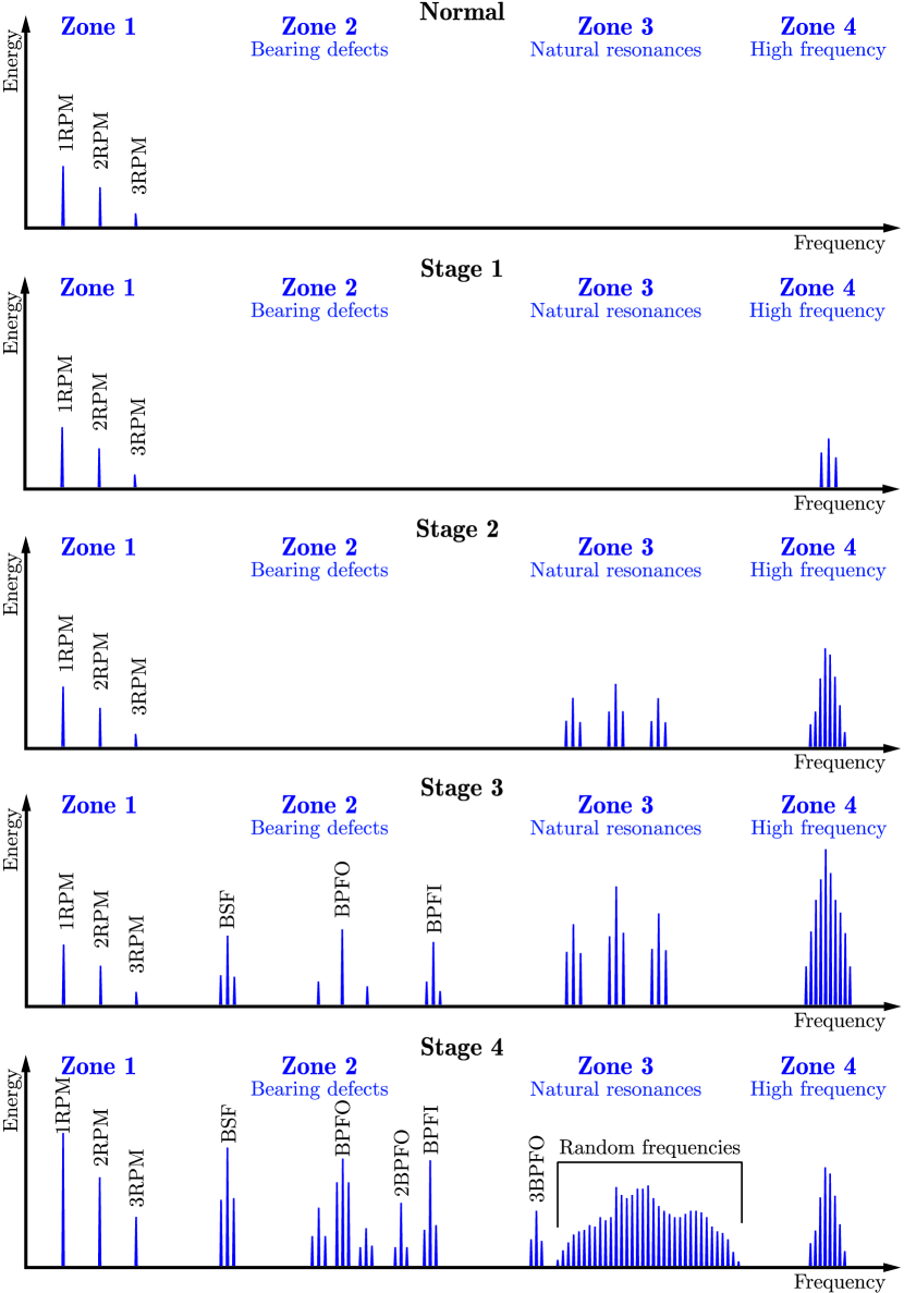
Figure 2: Evolution of the frequency spectrum across the stages of a typical bearing failure. Initially, a healthy bearing exhibits frequencies solely linked to shaft phenomena, such as balance or misalignment. Stage 1 introduces ultrasonic frequencies detectable only by specialized sensors, without visible defects on the bearing. Stage 2 is marked by signals aligning with the bearing parts’ natural resonance, alongside the initial appearance of defects upon inspection. Stage 3 features the fundamental defect frequencies and their harmonics, modulated by the shaft speed, indicating a spread of defects. Stage 4 is the final stage and precedes complete failure. This final stage is characterized by a mix of modulated fundamental frequencies, harmonics, and, ultimately, a shift towards a random noise floor.

3.3 Elements of survival analysis

We define a survival problem by a sequence of observations represented as triplets ($\bm{x}_{i}$, $t_{i}$, $\delta_{i}$), where $\bm{x}_{i}\in\mathbb{R}^{d}$ is a feature vector, $t_{i}$ denotes the time to event or censoring, and $\delta_{i}$ is the binary event indicator. Moreover, let $c_{i}$ denote the censoring time and $e_{i}$ denote the event time for the $i$th record, thus $t_{i}=e_{i}$ if $\delta_{i}=1$ or $t_{i}=c_{i}$ if $\delta_{i}=0$. We treat the survival time as discrete and limit the time horizon to a finite duration, denoted $(0,...,T_{max})$, where $T_{max}$ represents a predefined maximum time point (e.g., 1 year). A survival model then estimates the probability that the event of interest occurs at time $T$ later than $t$, that is, the survival probability $S\left(t\right)=\text{P}\left(T>t\right)=1-\text{P}\left(t\leq T\right)$. To estimate the survival probability, we use the hazard function:

$$h\left(t\right)=\lim_{\Delta t\rightarrow 0}\text{P}\left(t<T\leq t+\Delta t|T>t\right)/\Delta t\text{,}$$ (5)

which represents the failure rate at an instant after time $t$, assuming survival beyond that time [22, Ch. 11]. The hazard function is related to the survival function through $h\left(t\right)=f\left(t\right)/S\left(t\right)$, where $f\left(t\right)$ is the probability density associated with $T$. Formally, $f\left(t\right):=\lim_{\Delta t\rightarrow 0}\text{P}\left(t<T\leq t+\Delta t\right)/\Delta t$, that is, the instantaneous failure rate at time $t$. Under this definition, the function $h\left(t\right)$ is the probability density of $T$ conditioned on $T>t$, where the higher the value of $h\left(t\right)$, the higher the probability of failure. The functions $S\left(t\right)$, $h\left(t\right)$, and $f\left(t\right)$, are different but related ways to describe the probability distribution of $T$.

3.4 Elements of uncertainty estimation

Many machine learning methods for RUL prediction are indeed nonprobabilistic; they can only provide a point estimate of the RUL and disregard the inherent uncertainty associated with the prediction. The Bayesian framework is a theoretical approach that models uncertainty when estimating model parameters (epistemic) and when making the actual prediction (aleatoric) [41]. This allows us to assess confidence in the predictive results, which further encourages the adoption of the model as a decision support tool. In addition, it also offers effective tools to mitigate overfitting [21]. [44] introduced Bayesian Neural Networks (BNNs) for bearing health prognostics with uncertainty estimation to predict the RUL of turbofan engines. In a BNN, the weights are treated as a set of random variables $\bm{\theta}\sim\text{P}\left(\bm{\theta}\right)$. Let $\mathcal{D}$ denote the data, $\text{P}\left(\mathcal{D}|\bm{\theta}\right)$ the likelihood and $\text{P}\left(\bm{\theta}\right)$ the prior distribution over the parameter of interest $\bm{\theta}$. Bayesian inference computes the posterior distribution $\text{P}\left(\bm{\theta}|\mathcal{D}\right)=\text{P}\left(\bm{\theta}\right)\text{P}\left(\mathcal{D}|\bm{\theta}\right)/\text{P}\left(\bm{\theta}\right)$, and then obtains the predictive distribution of unobserved data conditioned on $\mathcal{D}$ by marginalizing over the parameter space $\Theta$, i.e., $\text{P}\left(\bm{x}_{\text{new}}|\mathcal{D}\right)=\int_{\Theta}\text{P}\left(\bm{x}_{\text{new}}|\mathcal{D},\bm{\theta}\right)\text{P}\left(\bm{\theta}|\mathcal{D}\right)\text{d}\bm{\theta}$. However, the posterior cannot be directly computed due to $\text{P}\left(\mathcal{D}\right)$ being intractable, and sampling methods do not scale well in high dimensions. To this end, variational inference (VI) has been proposed to approximate the posterior with a tractable parametric distribution, $q_{\bm{\zeta}}\left(\bm{\theta}\right)$. This $q_{\bm{\zeta}}\left(\bm{\theta}\right)$ is chosen within a class of tractable parametric distributions, $\mathcal{Q}$, by minimizing the KL divergence from $q_{\bm{\zeta}}\left(\bm{\theta}\right)$ to $\text{P}\left(\bm{\theta}|\mathcal{D}\right)$. In many modern neural networks, Monte Carlo Dropout (MCD) or another timely technique is used to approximate the VI solution [21]. [38] proposed BNNs as a tool for uncertainty estimation in survival analysis models using MCD and showed a performance advantage in adopting the Bayesian framework, especially in small datasets. The intrinsic probabilistic dimension of BNNs naturally allows us to make uncertainty estimates, estimate predictive errors, and plot credible intervals [47].

4 Methods and materials

4.1 The dataset

We use the accelerated degradation bearing dataset from Xi’an Jiaotong University (XJTU-SY) to evaluate the performance of our proposed method [62]. The dataset is generated from 15 deep grove ball bearings with a dynamic load rating of 12.82 kN. Three tests are performed with different loads and speeds (C1, C2, and C3), and five bearings are used in each test (see Tab. 1 and 2). During the test, each bearing is instrumented with two piezoelectric accelerometers, mounted horizontally ($X$-axis) and vertically ($Y$-axis), and vibrations are captured at a sampling frequency of 25.6 kHz. We sample only from the $X$-axis as suggested by [62]. 32.768 samples are recorded every minute. All bearings are run to failure under very high loads to accelerate degradation. This significantly increases the risk of initiating bearing defects but also comes with the risk of local flash heating and subsequent uncontrolled damage to a bearing.

Operating condition $L_{10h}$ [h] Radial force [kN] Rotating speed [rpm] Bearing dataset C1 9.6 12.0 2100 Bearing 1_1 to 1_5 C2 11.7 11.0 2250 Bearing 2_1 to 2_5 C3 14.6 10.0 2400 Bearing 3_1 to 3_5

Table 1: Overview of the XJTU-SY dataset.

Property Value Property Value Outer race diameter 39.80 mm Inner race diameter 29.30 mm Bearing mean diameter 34.55 mm Ball diameter 7.92 mm Number of balls 8 Contact angle 0$\degree$ Load rating (static) 6.65 kN Load rating (dynamic) 12.82 kN

Table 2: Properties of the LDK UER204 type bearings.

4.2 Feature extraction

We extract several features in the time domain from the raw bearing signal as important indicators to detect bearing degeneration [58]. These include peak amplitude, energy, rise time, time, RMS, skewness, kurtosis, and crest factor among others. In practice, the feature data come from an accelerometer placed on the ball bearings at an angle of 90 degrees. We recorded a total of 12 time domain features for the analysis, which are summarized in Table 3.

Feature name	Expression
Absolute mean ($\bar{x}$)	$\frac{1}{N}\sum_{i=1}^{N}\left|x_{i}\right|$
Standard deviation ($\sigma$)	$(\frac{1}{N}\sum_{i=1}^{N}(x_{i}-\mu)^{2})^{1/2}$
Skewness	$\frac{1}{N}\sum_{i=1}^{N}(x_{i}-\mu)^{3}/\sigma^{3}$
Kurtosis	$\frac{1}{N}\sum_{i=1}^{N}(x_{i}-\mu)^{4}/\sigma^{4}$
Entropy	$-\sum_{i=1}^{N}P(x_{i})\log P(x_{i})$
Root mean square (RMS)	$(\frac{1}{N}\sum_{i=1}^{N}x_{i}^{2})^{1/2}$
Max value	$\max(|\bm{x}|)$
Peak-To-Peak (P2P)	$\max(|\bm{x}|)-\min(|\bm{x}|)$
Crest factor	$\max(|\bm{x}|)/(\frac{1}{N}\sum_{i=1}^{N}x_{i}^{2})^{1/2}$
Clearance factor	$\max(|\bm{x}|)/(\frac{1}{N}\sum_{i=1}^{N}|x_{i}|^{1/2})^{2}$
Shape factor	$(\frac{1}{N}\sum_{i=1}^{N}x_{i}^{2})^{1/2}/\bar{x}$
Impulse	$\max(|\bm{x}|)/\bar{x}$

Table 3: Selected time domain features expressed in relation to the sampled signal $\bm{x}=(x)_{i=1}^{N}$. For convenience, $\mu$ stands for the mean value of $\bm{x}$.

4.3 Event detection algorithm

Algorithm 1 Event detection algorithm.

1:Signal $\bm{x}$, end of life $L$, and sensitivity $\lambda_{KL}$.  

2:Initialize $T=600$, $\eta=5$, $W=L-T$

3:Initialize event times $\bm{t}=[t_{1},t_{2},\ldots,t_{5}]=L\cdot\mathbbm{1}$

4:Compute the HT and FFT $\bm{z}=|FFT(H(\bm{x}))|$

5:for all critical band, $cb$, in $CB$ do

6:     Apply band-pass filter $\bm{z}_{cb}=BPF_{cb}(\bm{z})$

7:     $detected=\text{False}$

8:     $w=0$

9:     Initialize list $\bm{\Delta_{KL}}=[\;]$

10:     Initialize $\Delta_{KL}=0$

11:     while not $detected$ and $w\leq W$ do

12:         Extract window $\bm{z}_{cb}^{w}\leftarrow\bm{z}_{cb}$

13:         Estimate PDF $P_{w}(z)=\text{PDF}(\bm{z}_{cb}^{w})$

14:         if $w>0$ then

15:              Calculate $KL_{w}$ = $\sum_{z\in Z}P_{w}(z)\log\frac{P_{w}(z)}{P_{0}(z)}$

16:              if $w>1$ then

17:                  $\Delta_{KL}$ = $KL_{w}$ - $KL_{w-1}$

18:              end if

19:              $\bm{\Delta_{KL}}\leftarrow\Delta_{KL}$

20:              if $w>5$ then

21:                  Calculate $\sigma_{KL}$ as the SD($\bm{\Delta_{KL}}$)

22:                  Calculate $THS=th_{KL}(w,\eta,\sigma_{KL},L,\lambda_{KL})$

23:                  if $|\Delta_{KL}|>THS$ thens

24:                       $detected=\text{True}$

25:                       $\bm{t}_{cb}=w$

26:                  end if

27:              end if

28:         end if

29:         $w=w+1$

30:     end while

31:end for

32:$t_{event}\leftarrow min(\bm{t})$

33:return $t_{event}$

In this paper, we propose an event detection algorithm to estimate the time of predictive maintenance before failure occurs, which we later use as an oracle to label the XJTU-SY dataset. The main motivation of our proposed algorithm stems from the idea that the recorded end of life, $L$, of the bearing constitutes an overestimation of the time when the bearing actually breaks. In other words, the bearing usually starts to malfunction earlier than the time when the bearing becomes useless and the recording is stopped, and therefore, providing an inaccurate estimate of the breaking time is problematic because it can further bias the analysis.

In Algorithm (1), we present the pseudo-code of our proposed event detection algorithm. In summary, the algorithm first performs the Hilbert transform and then applies the FFT. This preliminary step is necessary to remove unwanted frequency components and eases the identification of the frequency bands of interest, as we explained in Sec. 3.1. The algorithm then systematically processes the signal obtained using a bandpass filter over the set of critical bands $CB=(cb_{i})_{i=1}^{5}$, as discussed in Sec. 3.1 and calculated based on the specific bearing properties of the XJTU-SY dataset in Tab. 2.

For every critical band, the algorithm segments the observed time series into $W$ window frames, each with a constant duration of $T=600$ seconds. Then, the KL divergence relative to the preceding window is calculated. Following this, the algorithm tracks the variations in the differences between these values until they surpass a specific threshold. When the difference exceeds this threshold, the algorithm detects an event for the current critical band at the current window, signaling that the bearing’s functioning has been compromised. For completeness, Figure 3 visualize the behavior of the algorithm for a particular critical band.

Regarding the threshold that controls the changes in the KL divergence, $th_{KL}(w)$, we defined this threshold function as an empirical model, drawing inspiration from the exponential deterioration model. Formally, it is defined as follows:

$$th_{KL}(w)=\eta\sigma_{KL}e^{-\beta t}\quad\text{with}\quad\beta=\frac{1}{L}\log\left(\frac{\eta}{\lambda_{KL}}\right),$$ (6)

where $w$ represents the window index, $L$ is the end of life, and $\sigma_{KL}$ is the estimated standard variation of the measured differences of the KL divergence between windows. Finally, $\eta$ and $\lambda_{KL}$ are two parameters that are linked to the bearing natural deterioration and bear a physical interpretation.

In particular, the parameter $\eta$ reflects the sensitivity of the approach to changes at the beginning of the recording, which is linked to the estimated standard variation, $\sigma_{KL}$. We recommend setting this parameter to $\eta=5$ since it is sufficient to account for any initial variations until the bearing reaches a steady state. Note that this parameter may be set to higher values, yet this value is enough to avoid initial nonstationary perturbations. On the other hand, $\lambda_{KL}\sim 1$ controls how sensitive the algorithm is when it is close to the end of the bearing life. Unlike $\eta$, this additional parameter may change depending on the particular condition of the experiment, since each condition affects the performance of the bearing. For this experiment, we set $\lambda_{KL}=1.5,1.75,2$ for the high, medium, and low load conditions, respectively.

Finally, note that $L$ indicates the end of life of the bearing. In this particular dataset, it corresponds to when the bearing becomes completely useless and the recording stops. In a real industrial scenario, we do not have access to this information since the actual failure of the bearing remains unknown. Nonetheless, we can use available similar information such as the $L_{10}$. As detailed in Sec. 3.1, this value provides valuable information regarding the actual lifetime expectancy of the bearing over a realistic scenario and can serve to fine-tune the proposed event detection algorithm.

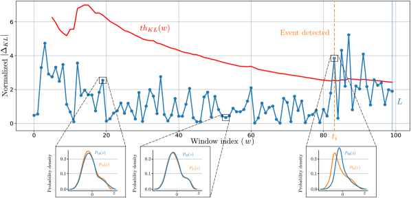
Figure 3: Visualization of the normalized $|\Delta_{KL}|$ and threshold function for a single critical band for the proposed event detection algorithm. This illustration depicts the segmentation of the signal into sequential windows ($w$), followed by the estimation of the KL divergence based on the estimated probability between consecutive windows. The diagram showcases some examples of the obtained probability density functions, and highlights the instance when the divergence exceeds the threshold, thereby indicating a probably significant malfunctioning of the bearing’s performance.

4.4 Data preprocessing and censoring

The XJTU-SY dataset is a tabular dataset, where the rows represent temporal covariate values and the columns represent covariate names. There are five bearings per operating condition and three operating conditions in total (see Tab. 1). As a preliminary preprocessing step, we convert the temporal dataset to a supervised learning dataset by computing a rolling average with adjustable window length ($w$) and lag ($l$) based on the operating condition. For bearings under high load (C1), we use $w=2/l=-1$, subsequently for medium load (C2), we use $w=4/l=-3$, and for light load (C3), we use $w=6/l=-5$. This reflects the length of the event horizon and means that more samples are gathered from bearings running for longer, but also that the averaging window is larger and the lag is higher. The moving window averages both the covariates ($\bm{X}_{i}$) and the event times ($\bm{t}_{i}$). This produces three supervised learning datasets, $\mathcal{D}_{C1}$ ($N=635$, $d=12$), $\mathcal{D}_{C2}$ ($N=1586$, $d=12$) and $\mathcal{D}_{C3}$ ($N=4930$, $d=12$), where $N$ is the number of samples and $d$ is the number of covariates.

In an industrial setting, censored observations would be bearings that are yet to fail. Because the XJTU-SY dataset only includes complete observations, i.e., the failure time is always known, we introduce random and independent censoring by a fixed percentage $C=\{25\%,50\%,75\%\}$. When applying censoring, if an observation $i$ is deemed censored, we use the time of censoring $c_{i}$ instead of the event time $e_{i}$ as the time to event, thus $t_{i}=c_{i}$ and $\delta_{i}=0$. Here, $c_{i}$ is a random number between the sampling time and the actual observed event time $e_{i}$. This indicates that the bearing was censored at some point in time between when it was recorded and when it failed. Figure 4 shows the Kaplan-Meier estimate and its upper and lower bounds after censoring has been applied to the individual datasets as a percentage. The bounds are the best/worst cases on the survival function given the observed data without any parametric assumptions. The bounds represent the extremes of what censoring is capable of doing to our estimates given the observed data. For the upper bound on the survival function, we assume that all censored bearings do not ever reach the event. For the lower bound, we assume that all censored bearings immediately reached the event after they were censored. Notice that the bounds get wider as more censoring occurs. Figure 5 shows a histogram of observed and censored events by operating condition.

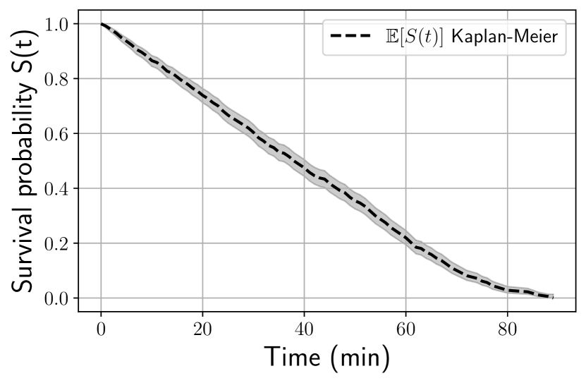
(a) Dataset $\mathcal{D}_{C1}$ - Censoring $25\%$

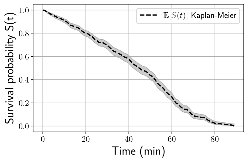
(b) Dataset $\mathcal{D}_{C1}$ - Censoring $50\%$

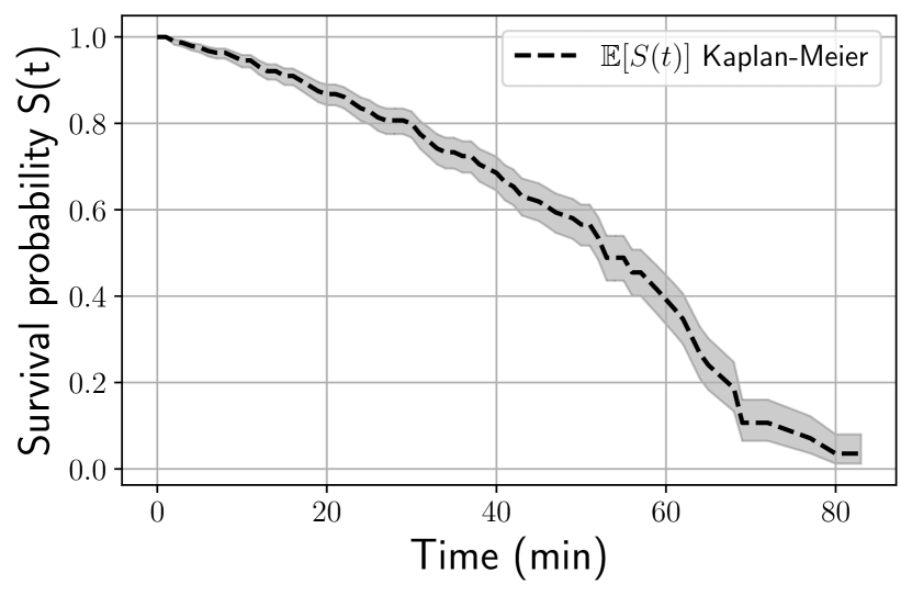
(c) Dataset $\mathcal{D}_{C1}$ - Censoring $75\%$

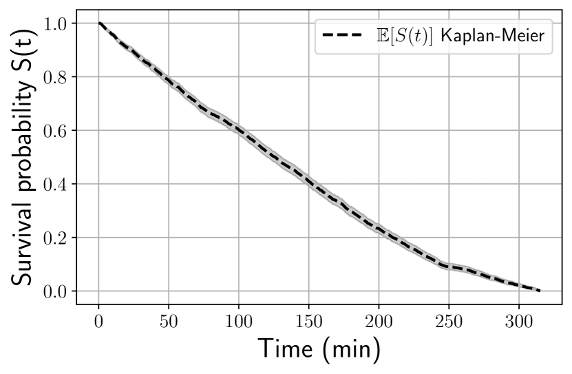
(d) Dataset $\mathcal{D}_{C2}$ - Censoring $25\%$

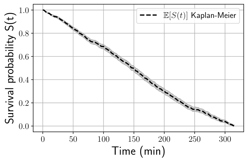
(e) Dataset $\mathcal{D}_{C2}$ - Censoring $50\%$

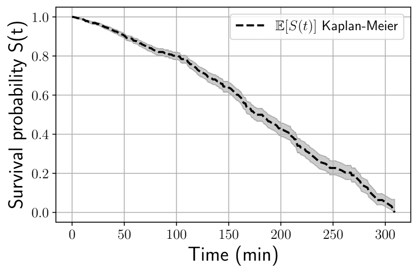
(f) Dataset $\mathcal{D}_{C2}$ - Censoring $75\%$

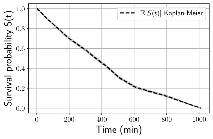
(g) Dataset $\mathcal{D}_{C3}$ - Censoring $25\%$

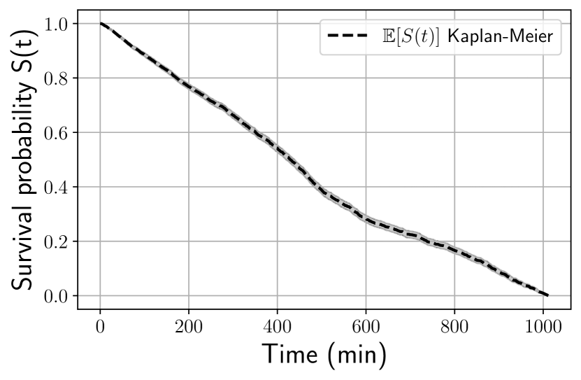
(h) Dataset $\mathcal{D}_{C3}$ - Censoring $50\%$

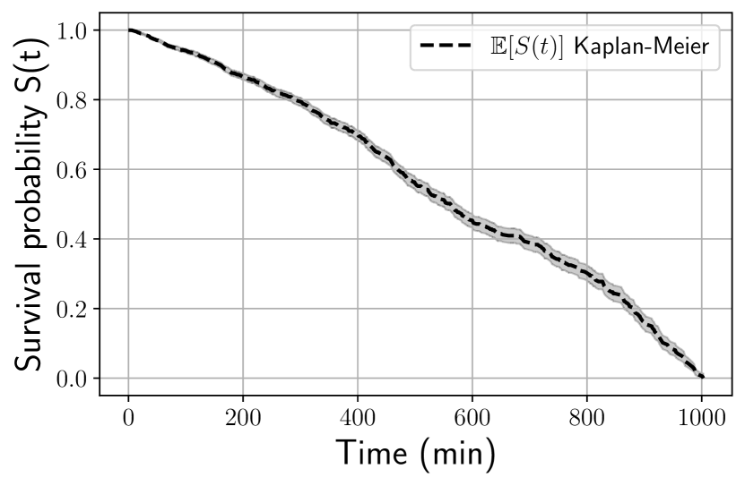
(i) Dataset $\mathcal{D}_{C3}$ - Censoring $75\%$

Figure 4: Predicted survival probability $S(t)$ by the Kaplan-Meier estimator with various amounts of censoring.

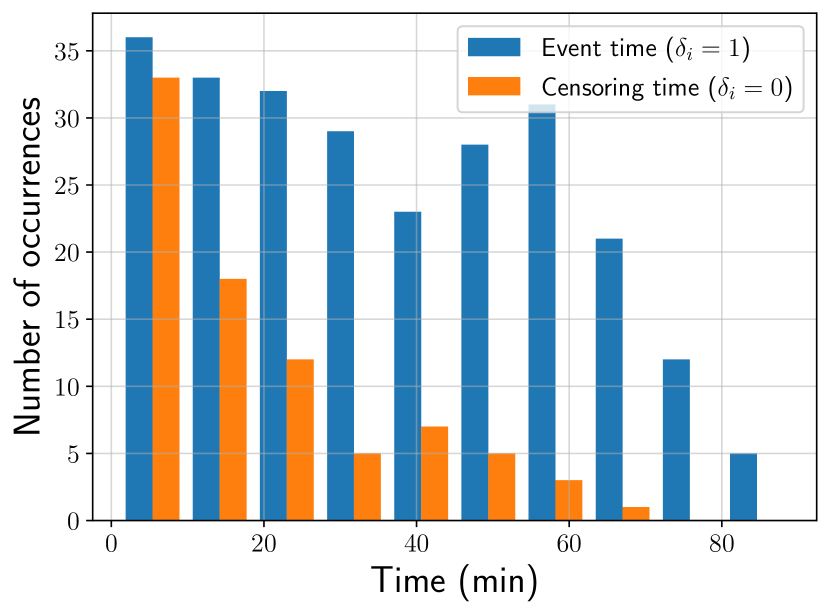
(a) Dataset $\mathcal{D}_{C1}$ - Censoring $25\%$

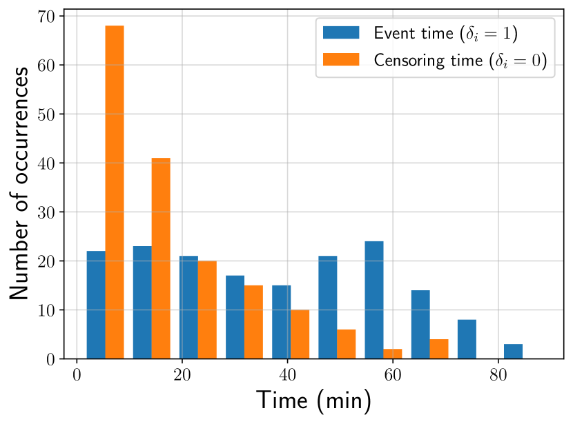
(b) Dataset $\mathcal{D}_{C1}$ - Censoring $50\%$

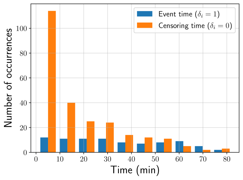
(c) Dataset $\mathcal{D}_{C1}$ - Censoring $75\%$

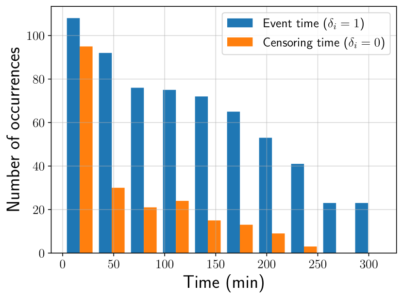
(d) Dataset $\mathcal{D}_{C2}$ - Censoring $25\%$

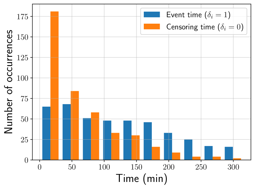
(e) Dataset $\mathcal{D}_{C2}$ - Censoring $50\%$

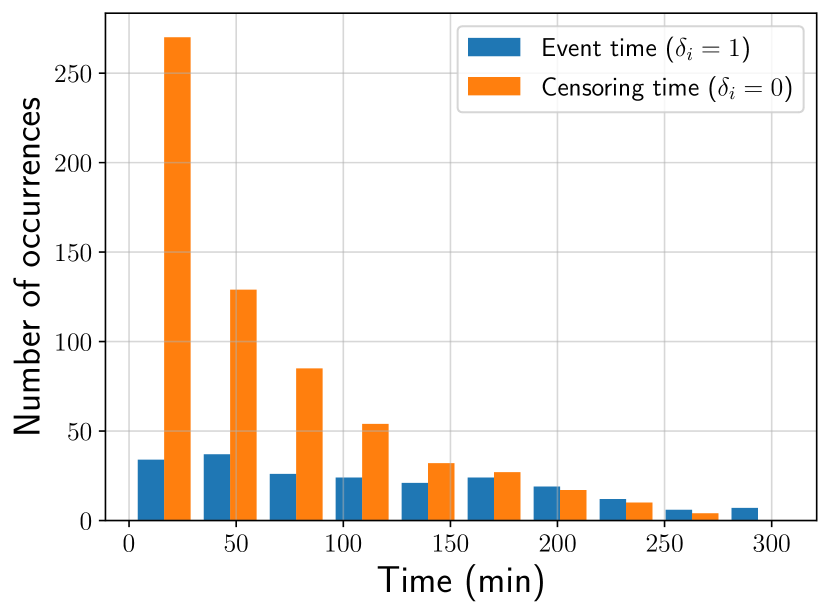
(f) Dataset $\mathcal{D}_{C2}$ - Censoring $75\%$

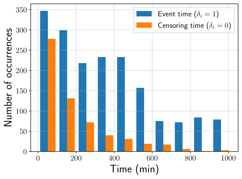
(g) Dataset $\mathcal{D}_{C3}$ - Censoring $25\%$

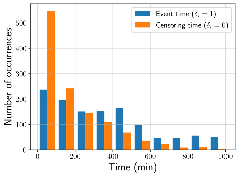
(h) Dataset $\mathcal{D}_{C3}$ - Censoring $50\%$

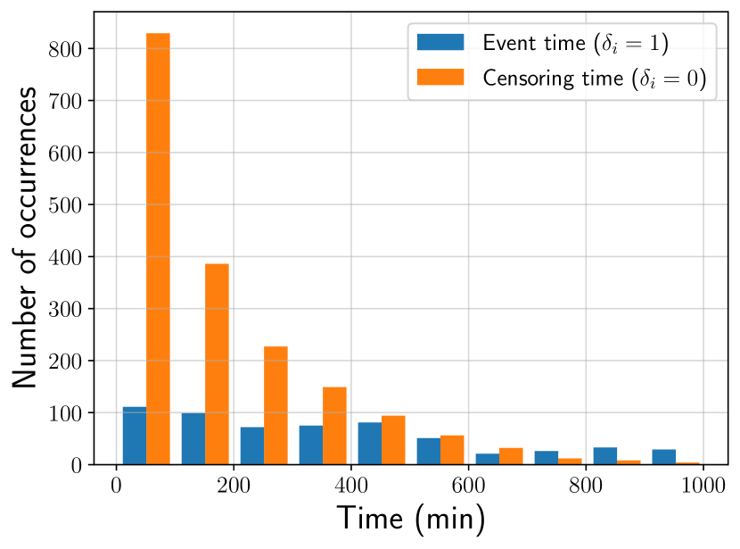
(i) Dataset $\mathcal{D}_{C3}$ - Censoring $75\%$

Figure 5: Event distribution with various amounts of censoring.

5 Experimental results and discussion

5.1 Setup

We implement the traditional Cox model (CoxPH) [13], CoxBoost [8], Random Survival Forests (RSF) [29], and two neural network-based models, Multi-Task Logistic Regression (MTLR) [72] and BNNSurv using Monte-Carlo Dropout (MCD) [38] (see Sec. A for details). To estimate the generalization error of each model, we arrange a stratified 5-fold cross-validation (5CV) procedure, which ensures that event times and censoring levels are consistent across each fold. For each fold, we apply $z$-score data normalization to all covariates, compute the event horizon on the training set and report model performance across the five folds in terms of predictive accuracy and calibration. If the model requires a validation set for early stopping, we allocate 30% of the training set for this purpose. For the continuous-time models (CoxPH, Coxboost, RSF, and BNNSurv), we compute the event horizon using the unique events and censoring times in the training set, thus the number of bins is the number of unique time points. For the discrete-time model (MTLR), we calculate the square root of the number of uncensored observations, $\sqrt{\sum_{i:\delta_{i=1}}\mathbbm{1}}$, in the training set and use quantiles to evenly divide these uncensored observations into bins, as in [26].

For the baseline CoxPH model, we adopt sensible defaults with a convergence criterion of $10^{-9}$ and a maximum of 100 iterations. For the CoxBoost and RSF models, according to the operating condition, we set the number of estimators to $\{100,200,400\}$, the minimum number of samples needed to split to $\{5,10,20\}$, the minimum number of samples in a leaf node to $\{3,5,10\}$, a maximum depth of $\{3,5,10\}$, and maximize the Cox partial log-likelihood (see Eq. A). For the MTLR model, we use batch sizes of $\{32,64,128\}$, hidden sizes of $\{16,32,64\}$, a fixed dropout rate of 0.25, a learning rate of 0.00008 using the Adam optimizer, a penalty term of 0.01, and 5000 training epochs as suggested by [47]. For the BNNSurv model, we use batch and network sizes similar to those of MTLR, but with a learning rate of 0.01 for the Adam optimizer and 100 epochs of training.

To evaluate predictive performance, we report the mean absolute error (MAE) using a Hinge loss (MAE_H) [46], the MAE using the margin time for censored observations (MAE_M) [46] and the MAE using surrogate event times (MAE_PO). To evaluate the calibration performance, we report the distribution calibration (D-Calibration) [26] and the coverage calibration (C-Calibration) [47] (see Sec. B for details).

5.2 Event detector

Table 4 shows a comparison between the annotated event times and the actual failure times in minutes. Observe that the average difference between the annotated end of life and the estimated time of the breaking of the bearing is 42.6%, 48.7%, and 56.9% for high, medium, and low load condition, respectively. Note that those percentages are relatively high, and all events are detected before the end of the recording, i.e., the time of failure. These results support the use of the proposed event detector since it seems to provide a better estimate of the time when each bearing starts to break but does not fail. Note that a bearing’s failure time in this scenario is when it has physically stopped working, so the event time, i.e., when the bearing starts malfunctioning, should be detected well in advance for predictive maintenance to have an effect.

It is also worth addressing that the bearings in the XJTU-SY dataset fail at entirely different times, although they are run under the same load. This points to other factors (e.g., temperature, lubrication, previous wear) having a significant influence on the lifetime. We do see an increasing average error for lighter loads, which can be mitigated further by adjusting $\lambda_{KL}$ for the event detector (see Alg. 1), to ensure a proper threshold for the KL divergence. In an industrial setting, bearings are normally run under a lot less stress than in this dataset, so the event detector would have to be recalibrated on any new dataset, bearing in mind the operational overhead predictive maintenance has, i.e., what is the cost of not detecting a failure in a faulty bearing (false negative), as opposed to detecting a failure in a healthy bearing (false positive).

Operating condition	Bearing dataset	$t_{i}$ [m]	$L$ [m]	Difference [m]	Difference [%]
C1 (high)	Bearing 1_1	77	122	-45	36.9
	Bearing 1_2	89	160	-71	44.4
	Bearing 1_3	62	157	-95	60.5
	Bearing 1_4	70	121	-51	42.1
	Bearing 1_5	36	51	-15	29.4
C2 (medium)	Bearing 2_1	245	490	-245	50.0
	Bearing 2_2	77	160	-83	51.9
	Bearing 2_3	316	532	-216	40.6
	Bearing 2_4	17	41	-24	58.5
	Bearing 2_5	193	338	-145	42.9
C3 (low)	Bearing 3_1	1014	2537	-1523	60.0
	Bearing 3_2	612	2495	-1883	75.5
	Bearing 3_3	206	370	-164	44.3
	Bearing 3_4	514	1514	-1000	66.1
	Bearing 3_5	69	113	-44	38.9

Table 4: Comparison of the annotated event time ($t_{i}$) detected by the proposed algorithm (see Sec. 4.3), and the end of life ($L$), i.e., the end of the recording, as reported in the dataset [62]. The last two columns show the difference and the percentage of the difference between the end of life and the time estimated by the detector. All values are expressed in minutes.

5.3 Model performance

Table 5 shows the experimental results from cross-validation in terms of prediction performance. Generally, we see better predictive performance under high load ($\mathcal{D}_{C1}$), where the event horizon is shorter, the bearings deteriorate faster, and the event times are much more consistent (see Tab. 4 and Fig. 5), compared to medium load ($\mathcal{D}_{C2}$) and low load ($\mathcal{D}_{C3}$). Under high load, increasing the level of censoring does not impact the MAE_H, but leads to worse MAE_M and MAE_PO scores, particularly under high censoring levels($C=75\%$). MAE_M and MAE_PO compute surrogate times or pseudo-observations [3, 4] for censored observations. Censoring increases the number of unobserved observations; thus, with more censoring comes more uncertainty. Consequently, the metric has to come up with artificial event times for more samples, which leads to higher predictive error. This trend is common to all models. The baseline CoxPH model gives acceptable MAE scores under high load ($\mathcal{D}_{C1}$), but cannot keep up with its ensemble and neural network-based variants when the sample space increases, only surpassing the CoxBoost model in terms of accuracy. The RSF model, a shallow model based on ensemble learning, performs the best across all datasets and censoring levels, even outperforming the neural networks, and its MAE_H score is stable at all censoring levels. Censoring appears to have a regularization effect on the neural networks, with better MAE_H scores as censoring increases, possibly preventing the model from overfitting the training data by introducing noise.

We also report the eMAE, which is the error between the MAE without censoring ($C=0$) and the MAE with censoring ($C>0$) in Table 6. Formally, the MAE estimator without censoring is often referred to as true MAE [46], and the eMAE can be any of the adopted MAE metrics that support censoring, i.e., $eMAE=\text{True MAE}-\text{MAE\textsubscript{H}/MAE\textsubscript{M}/MAE\textsubscript{PO}}$. Table 6 reports the eMAE for the respective datasets, models, and censoring levels. An eMAE above zero means that the censoring-MAE underestimates the true MAE, whereas an eMAE below zero means that the censoring-MAE overestimates it. We see that MAE_H tends to underestimate the true MAE, MAE_M gives good predictive estimates and MAE_PO tends to overestimate it. Increasing censoring naturally leads to larger fluctuations in the approximate true MAE, which is most pronounced in $\mathcal{D}_{C3}$. For completeness, Table 7 reports the true MAE without any censoring of the test data, although the models are still trained on censored data. As was the case when the test data contained censored observations, RSF boasts the lowest true MAE on average across all datasets. As a simple comparison, we also trained a linear model with a $\ell_{1}$ prior regularizer (LASSO) on uncensored observations only in the dataset, i.e., $\mathcal{D}^{\delta_{i=1}}$, which does not support censoring and thus disregards censored observations.

Table 8 shows the experimental results of cross-validation in terms of calibration performance (D-calibration and C-calibration). Given a predicted survival curve $S(t)$ by model $M$, we slice $S(t)$ into 10% intervals and accept the null hypothesis that the set $\{S_{i}(d_{i})\}$ is uniformly distributed between $[0,1]$ for all individual distributions $d_{i}$ if the $p$-value of a Pearson’s $\chi^{2}$ test is above 0.05. Well-calibrated models have $p$-values greater than 0.05. We can see from the table that all models pass the test in 5/5 folds in the $\mathcal{D}_{C1}$ dataset, except BNNSurv, when the load is heavy and the event horizon is short. As we decrease the load and the event horizon becomes longer, more models start to fail the calibration test, since the survival curves now have to match the Kaplan-Meier (KM) [32] probabilities over a longer time period. The MTLR is the only model that gives D-calibrated survival curves on all datasets, no matter the level of censoring. For BNNSurv, we check if the predicted credible intervals match the observed probability intervals, which is the case for all operating conditions and censoring levels.

Figure 6 shows the mean survival curves predicted by covariate-based models and the survival curve by the KM estimator. The KM estimator is a nonparametric method for estimating the survival function of a population based on the observed survival time. Here, we assess KM-calibration visually by observing the agreement between a model’s predicted survival probabilities and the observed survival probabilities. We assume censoring to be independent, that is, bearings are censored due to reasons unrelated to the event, which means the KM estimator is unbiased, regardless of the proportion of censoring. By visual inspection, we see that all models produce survival curves that align with the KM estimate.

Dataset	Method	25% censoring			50% censoring			75% censoring
		MAEH	MAEM	MAEPO	MAEH	MAEM	MAEPO	MAEH	MAEM	MAEPO
$\mathcal{D}_{C1}$ (high) ($N=635$, $d=12$)	CoxPH	14.1$\pm$1.7	14.8$\pm$1.7	15.0$\pm$1.6	13.0$\pm$1.7	14.5$\pm$1.8	15.5$\pm$2.3	11.9$\pm$2.6	14.2$\pm$2.5	20.7$\pm$4.4
	CoxBoost	16.9$\pm$1.5	17.7$\pm$1.5	18.0$\pm$1.5	16.7$\pm$1.6	18.0$\pm$1.6	19.1$\pm$1.9	17.3$\pm$4.3	18.9$\pm$4.4	25.9$\pm$6.0
	RSF	12.1$\pm$1.0	12.8$\pm$1.0	13.0$\pm$1.0	11.2$\pm$1.5	12.6$\pm$1.7	13.5$\pm$2.1	12.4$\pm$2.4	14.6$\pm$2.1	21.3$\pm$4.6
	MTLR	13.0$\pm$1.3	13.7$\pm$1.4	13.8$\pm$1.3	11.9$\pm$2.6	13.3$\pm$2.6	14.2$\pm$2.9	13.5$\pm$2.4	16.0$\pm$2.4	22.6$\pm$5.0
	BNNSurv	12.9$\pm$1.6	13.6$\pm$1.7	13.7$\pm$1.7	12.3$\pm$2.9	13.8$\pm$3.0	14.7$\pm$3.4	12.1$\pm$1.8	14.4$\pm$1.9	21.2$\pm$4.3
$\mathcal{D}_{C2}$ (medium) ($N=1586$, $d=12$)	CoxPH	52.8$\pm$4.1	55.7$\pm$4.0	56.7$\pm$4.0	50.0$\pm$1.6	56.6$\pm$1.5	63.0$\pm$2.6	51.5$\pm$14.4	62.3$\pm$14.1	89.9$\pm$17.9
	CoxBoost	57.4$\pm$3.1	60.7$\pm$2.9	61.8$\pm$2.7	58.1$\pm$4.0	65.2$\pm$3.7	71.9$\pm$4.7	61.6$\pm$6.8	71.5$\pm$7.1	100.0$\pm$10.7
	RSF	29.4$\pm$2.2	32.7$\pm$2.4	33.4$\pm$2.6	29.8$\pm$4.4	36.8$\pm$4.0	42.5$\pm$4.9	31.8$\pm$7.3	43.1$\pm$7.0	69.9$\pm$13.3
	MTLR	47.0$\pm$5.4	49.9$\pm$5.2	50.7$\pm$5.0	45.5$\pm$2.6	52.3$\pm$3.0	58.2$\pm$3.8	42.8$\pm$6.3	54.5$\pm$6.5	81.6$\pm$12.2
	BNNSurv	41.8$\pm$9.2	44.7$\pm$9.0	45.6$\pm$8.9	42.1$\pm$1.6	49.2$\pm$1.9	55.6$\pm$2.0	38.5$\pm$6.3	52.9$\pm$6.2	81.3$\pm$12.3
$\mathcal{D}_{C3}$ (low) ($N=4930$, $d=12$)	CoxPH	173.9$\pm$8.4	185.9$\pm$7.8	189.8$\pm$7.9	164.6$\pm$10.2	192.2$\pm$8.7	217.7$\pm$7.8	196.8$\pm$27.1	236.1$\pm$24.5	330.3$\pm$35.5
	CoxBoost	188.7$\pm$3.2	202.3$\pm$2.9	206.3$\pm$3.3	189.2$\pm$9.6	218.8$\pm$7.8	245.1$\pm$6.3	205.6$\pm$11.1	246.5$\pm$11.0	342.6$\pm$20.5
	RSF	98.8$\pm$7.3	110.2$\pm$6.6	113.1$\pm$7.5	96.7$\pm$6.2	123.6$\pm$5.2	146.6$\pm$5.9	96.3$\pm$12.9	141.9$\pm$13.7	230.8$\pm$23.1
	MTLR	143.4$\pm$7.7	155.4$\pm$7.1	158.6$\pm$7.1	139.2$\pm$8.2	166.9$\pm$7.1	190.2$\pm$6.9	137.2$\pm$15.4	182.2$\pm$14.6	267.9$\pm$25.4
	BNNSurv	133.7$\pm$6.8	145.5$\pm$6.4	149.2$\pm$6.9	125.9$\pm$9.2	156.1$\pm$7.6	181.9$\pm$6.9	122.2$\pm$8.2	181.2$\pm$8.0	277.3$\pm$19.6

Table 5: Mean and standard deviation of MAE_H, MAE_M and MAE_PO, averaged over 5 folds. Note that lower values indicate better predictive accuracy.

Dataset	Method	25% censoring			50% censoring			75% censoring
		eMAEH	eMAEM	eMAEPO	eMAEH	eMAEM	eMAEPO	eMAEH	eMAEM	eMAEPO
$\mathcal{D}_{C1}$ (high) ($N=635$, $d=12$)	CoxPH	0.6$\pm$0.7	-0.2$\pm$0.7	-0.3$\pm$0.6	2.5$\pm$0.9	0.9$\pm$1.1	0.0$\pm$1.4	5.5$\pm$2.8	3.1$\pm$2.6	-3.4$\pm$4.5
	CoxBoost	0.5$\pm$0.6	-0.3$\pm$0.6	-0.6$\pm$0.5	2.7$\pm$0.8	1.5$\pm$0.8	0.3$\pm$0.9	5.7$\pm$4.3	4.1$\pm$4.3	-2.9$\pm$5.1
	RSF	0.5$\pm$0.5	-0.3$\pm$0.5	-0.4$\pm$0.4	2.9$\pm$0.7	1.4$\pm$0.9	0.5$\pm$1.2	4.8$\pm$2.2	2.6$\pm$1.9	-4.1$\pm$3.7
	MTLR	0.8$\pm$0.6	0.1$\pm$0.7	0.0$\pm$0.6	2.7$\pm$0.8	1.3$\pm$0.9	0.5$\pm$1.3	4.0$\pm$2.3	1.6$\pm$2.2	-5.0$\pm$4.1
	BNNSurv	0.7$\pm$0.8	-0.1$\pm$0.9	-0.2$\pm$0.9	2.3$\pm$1.4	0.7$\pm$1.5	-0.1$\pm$1.8	4.9$\pm$2.3	2.7$\pm$2.2	-4.2$\pm$4.6
$\mathcal{D}_{C2}$ (medium) ($N=1586$, $d=12$)	CoxPH	3.5$\pm$1.6	0.6$\pm$1.6	-0.3$\pm$1.6	7.1$\pm$1.5	0.5$\pm$1.4	-5.9$\pm$0.7	18.9$\pm$3.7	8.1$\pm$3.8	-19.6$\pm$7.0
	CoxBoost	3.3$\pm$0.6	0.0$\pm$0.5	-1.0$\pm$0.7	8.9$\pm$3.7	1.8$\pm$3.3	-4.8$\pm$4.1	20.3$\pm$1.1	10.4$\pm$1.2	-18.1$\pm$7.9
	RSF	2.1$\pm$0.6	-1.2$\pm$0.8	-1.9$\pm$1.1	4.5$\pm$1.3	-2.5$\pm$1.4	-8.2$\pm$1.4	11.4$\pm$1.6	0.1$\pm$1.6	-26.7$\pm$7.1
	MTLR	3.9$\pm$2.2	1.0$\pm$2.1	0.1$\pm$2.1	7.7$\pm$1.8	0.9$\pm$1.9	-5.1$\pm$1.1	16.3$\pm$3.4	4.6$\pm$3.6	-22.4$\pm$9.5
	BNNSurv	2.2$\pm$1.6	-0.8$\pm$1.6	-1.7$\pm$1.7	5.3$\pm$2.2	-1.8$\pm$2.2	-8.2$\pm$1.7	12.0$\pm$3.3	-2.4$\pm$3.4	-30.8$\pm$9.1
$\mathcal{D}_{C3}$ (low) ($N=4930$, $d=12$)	CoxPH	9.8$\pm$2.9	-2.2$\pm$2.4	-6.1$\pm$2.4	26.1$\pm$4.7	-1.6$\pm$3.2	-27.0$\pm$2.5	68.7$\pm$9.6	29.4$\pm$10.9	-64.8$\pm$18.7
	CoxBoost	8.7$\pm$2.8	-4.9$\pm$2.5	-8.9$\pm$2.4	27.0$\pm$5.7	-2.6$\pm$3.9	-29.0$\pm$2.6	65.2$\pm$9.9	24.4$\pm$10.2	-71.8$\pm$17.2
	RSF	6.5$\pm$2.0	-4.8$\pm$2.1	-7.8$\pm$2.6	14.0$\pm$3.0	-12.9$\pm$3.4	-35.9$\pm$2.8	39.9$\pm$12.0	-5.7$\pm$12.5	-94.6$\pm$23.1
	MTLR	8.3$\pm$2.7	-3.7$\pm$2.1	-7.0$\pm$2.5	19.8$\pm$2.7	-7.9$\pm$3.0	-31.2$\pm$2.5	53.9$\pm$9.8	8.9$\pm$9.1	-76.9$\pm$22.2
	BNNSurv	7.4$\pm$3.0	-4.5$\pm$2.4	-8.2$\pm$2.5	15.5$\pm$4.3	-14.7$\pm$4.0	-40.5$\pm$3.0	27.8$\pm$4.9	-31.2$\pm$5.6	-127.3$\pm$19.3

Table 6: Mean and standard deviation of eMAE, i.e., the difference between the MAE without censoring and the MAE with censoring, averaged over 5 folds. Note that lower values of eMAE indicates that the error is closer to the true MAE.

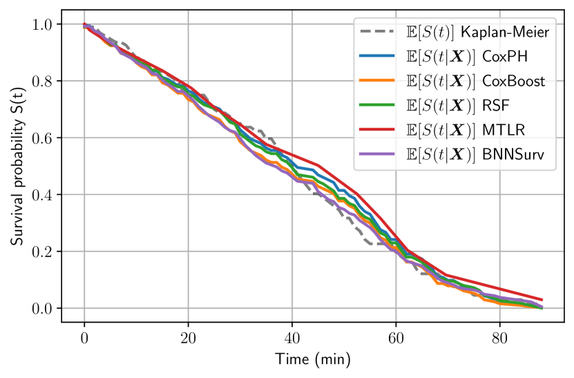
(a) $\mathcal{D}_{C1}$ (high).

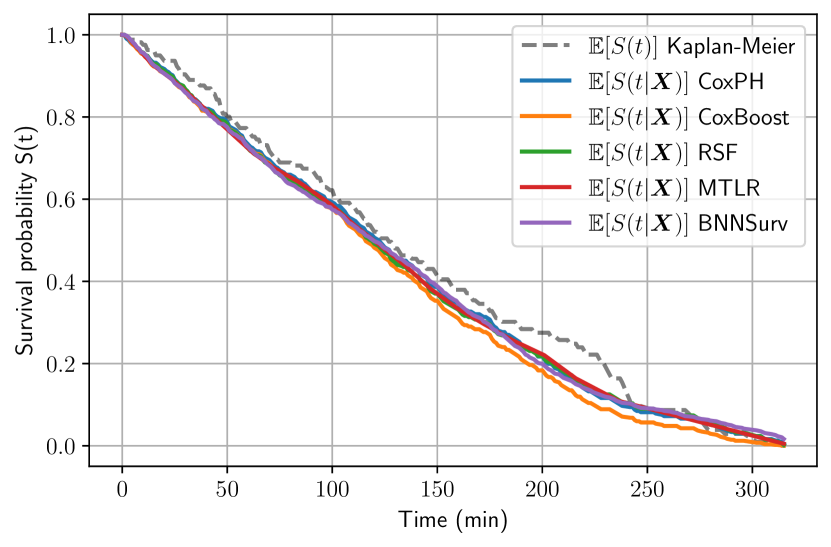
(b) $\mathcal{D}_{C2}$ (medium).

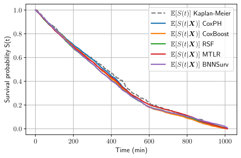
(c) $\mathcal{D}_{C3}$ (low).

Figure 6: Predicted mean survival curves by dataset, where 70% was used for training and 30% for testing with $C=25\%$. Solid lines: covariate-based models; Dashed line: Kaplan-Meier [32] estimator). The covariate-based models should predict survival curves that align with Kaplan-Meier on average.

Dataset	Method	True MAE
		$C=25\%$	$C=50\%$	$C=75\%$
$\mathcal{D}_{C1}$ (high) ($N=635$, $d=12$)	LASSO∗	18.5$\pm$1.1	19.6$\pm$0.8	19.7$\pm$1.3
	CoxPH	14.7$\pm$1.1	15.5$\pm$1.5	17.3$\pm$0.7
	CoxBoost	17.4$\pm$1.5	19.5$\pm$1.5	23.0$\pm$1.5
	RSF	12.6$\pm$0.8	14.0$\pm$1.7	17.2$\pm$1.2
	MTLR	13.8$\pm$1.1	14.6$\pm$2.4	17.5$\pm$2.4
	BNNSurv	13.5$\pm$1.0	14.6$\pm$2.0	17.1$\pm$1.8
$\mathcal{D}_{C2}$ (medium) ($N=1586$, $d=12$)	LASSO∗	63.0$\pm$3.6	64.8$\pm$4.0	65.0$\pm$3.2
	CoxPH	56.4$\pm$3.8	57.1$\pm$2.9	70.3$\pm$14.6
	CoxBoost	60.8$\pm$3.0	67.0$\pm$2.0	81.9$\pm$6.3
	RSF	31.5$\pm$2.0	34.3$\pm$4.5	43.2$\pm$7.0
	MTLR	50.9$\pm$4.1	53.1$\pm$3.9	59.1$\pm$5.3
	BNNSurv	44.0$\pm$9.5	47.4$\pm$3.3	50.5$\pm$4.9
$\mathcal{D}_{C3}$ (low) ($N=4930$, $d=12$)	LASSO∗	206.4$\pm$5.1	209.9$\pm$8.4	224.0$\pm$6.1
	CoxPH	183.7$\pm$6.2	190.6$\pm$5.9	265.5$\pm$34.2
	CoxBoost	197.4$\pm$2.6	216.2$\pm$4.2	270.8$\pm$5.2
	RSF	105.3$\pm$6.2	110.7$\pm$7.5	136.2$\pm$1.9
	MTLR	151.7$\pm$6.6	159.0$\pm$8.2	191.0$\pm$6.4
	BNNSurv	141.1$\pm$5.3	141.4$\pm$8.1	150.0$\pm$3.9

Table 7: Mean and standard deviation of the true MAE, averaged over 5 folds. $C$ is the level of censoring. ^∗Linear model trained with a $\ell_{1}$ prior regularizer (LASSO) on non-censored observations only.

Dataset	Method	25% censoring		50% censoring		75% censoring
		D-Cal	C-Cal	D-Cal	C-Cal	D-Cal	C-Cal
$\mathcal{D}_{C1}$ (high) ($N=635$, $d=12$)	CoxPH	5/5	-	5/5	-	5/5	-
	CoxBoost	5/5	-	5/5	-	5/5	-
	RSF	5/5	-	5/5	-	5/5	-
	MTLR	5/5	-	5/5	-	5/5	-
	BNNSurv	4/5	5/5	5/5	5/5	5/5	5/5
$\mathcal{D}_{C2}$ (medium) ($N=1586$, $d=12$)	CoxPH	5/5	-	5/5	-	5/5	-
	CoxBoost	4/5	-	5/5	-	5/5	-
	RSF	4/5	-	5/5	-	5/5	-
	MTLR	5/5	-	5/5	-	5/5	-
	BNNSurv	4/5	5/5	5/5	5/5	5/5	5/5
$\mathcal{D}_{C3}$ (low) ($N=4930$, $d=12$)	CoxPH	3/5	-	5/5	-	5/5	-
	CoxBoost	5/5	-	5/5	-	5/5	-
	RSF	0/5	-	3/5	-	5/5	-
	MTLR	5/5	-	5/5	-	5/5	-
	BNNSurv	0/5	5/5	0/5	5/5	0/5	5/5

Table 8: Number of D-calibrated mean survival curves and C-calibrated individual survival distributions over 5 folds according to a Pearson’s $\chi^{2}$ goodness-of-fit test. Calibrated models have $p$-values greater than 0.05. C-calibration is only applicable for models that can predict credible regions (CrIs) [47].

5.4 Stratified survival curves

Figure 7 shows the predicted mean survival curve and two survival curves when predicting on a stratified set of covariates in the $\mathcal{D}_{C1}$ dataset with 25% random censoring. This stratification is based on the 0.25, 0.5, and 0.75 quantiles from left to right. Recall that survival probability, $S(t)$, is the probability that the event occurs later than time $t$, so higher values are associated with lower predicted risk. We see that the predicted survival curves have notable differences based on the covariate and that some covariate values lead to significantly shorter predicted lifetimes. In fact, across all evaluated covariates in this plot, the RSF model produces more favorable survival outcomes when the value is below the median and unfavorable when it is above (center column in Fig. 7). For example, the root-mean-square (RMS) value represents the amount of energy in a signal. As a bearing starts to deteriorate, the RMS value will increase (center row in Fig. 7). This happens because the number of peaks increases, thus affecting the total signal energy.

Typically, during the initial phases of mechanical failure, the RMS value exhibits minimal alteration due to the limited shift in total signal energy. However, as failures progress, RMS tends to show a more pronounced increase. This way of stratification can provide insight into the learned representation between the inputs and the outputs and to create counterfactual explanations: if the energy of the signal was less, the bearing would have failed later.

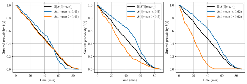
(a) The ”mean” covariate stratified by the 0.25, 0.5 and 0.75 quantiles.

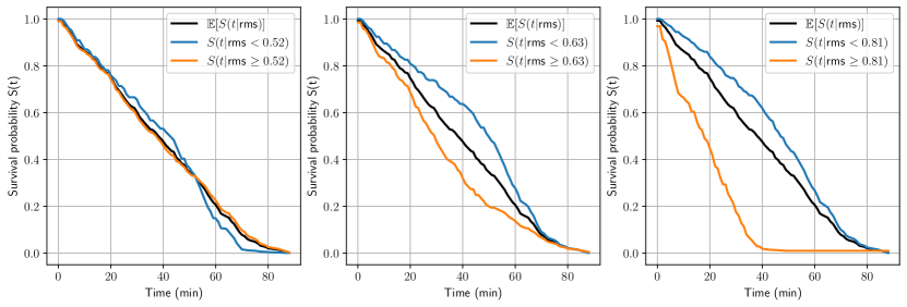
(b) The ”rms”” covariate stratified by the 0.25, 0.5 and 0.75 quantiles.

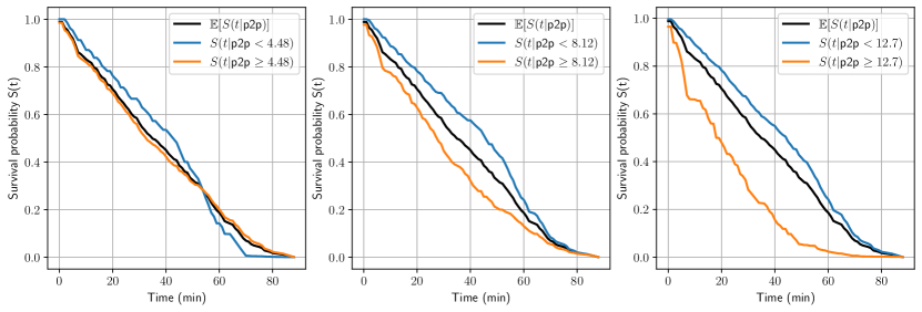
(c) The ”p2p” covariate stratified by the 0.25, 0.5 and 0.75 quantiles.

Figure 7: Predicted survival curves over a stratified set of covariates using the RSF model [29] (Black line: the mean predicted survival function without stratification; Blue line: the predicted survival function for bearings with covariates below the respective quantile; Orange line: the predicted survival function for bearings with covariates above). We set $C=25\%$ and train the model on the $\mathcal{D}_{C1}$ dataset, where 80% of the data is used for training and 20% for testing. The curves are plotted only for the test set.

5.5 Individual RUL prediction

We use BNNSurv to predict the RUL per bearing by estimating its individual survival distribution (ISD). The ISD is a representation of the estimated remaining useful life that a bearing has based on its covariates. For each operating condition $\{\mathcal{D}_{C1},\mathcal{D}_{C2},\mathcal{D}_{C3}\}$, we have a total of $N=5$ bearings, when sampling from the $X$-axis, as suggested by [62]. To predict the ISD of a single bearing, we train $M$ models, where $M$ is the number of operating conditions multiplied by the number of bearings. For example, to predict the ISD of the bearing $i,j$, where $i$ is the operating condition and $j$ is the bearing index, we train the model $M_{i,j}$ on the bearings $\mathcal{D}_{i}^{-j}$, where the notation $-j$ denotes that the dataset excludes the $j$th bearing, and predicts the ISD by taking a single sample from bearing $i,j$ at the beginning of its lifetime. This process is repeated iteratively for all bearings. Figure 8 shows the predicted mean survival curve and the upper and lower bounds of the credible intervals (CrIs), estimated by drawing 100 samples from the predictive distribution. We follow [47] and take the median of the survival curve (0.5) as the predicted time of the event $\hat{t}_{i}$ and compare that to the observed event time $t_{i}$. Although the event detector always detects the event of interest before the end of life (see Tab. 4), the RUL can be predicted before or after this point. We see a lot of uncertainty in many of the predictions (wide credible intervals), especially for C1 due to the low amount of training data available (left column), and there are many irregularities in the predicted RUL, especially for conditions C2 and C2 (center and right columns), which the model cannot reliably predict from just a single sample in this case. Ideally, the predicted time to event should match the actual time to event, and preferably before the end of life, so that predictive maintenance can be initiated in time. Depending on the industrial application and the cost of predictive maintenance, overestimating RUL is often worse than underestimating it. We emphasize the importance of calibrating the event algorithm, and the prediction models to depend on the operating condition, the environment, and the training scheme, and multiple predictions should be made at various time points to accurately predict a bearing’s health.

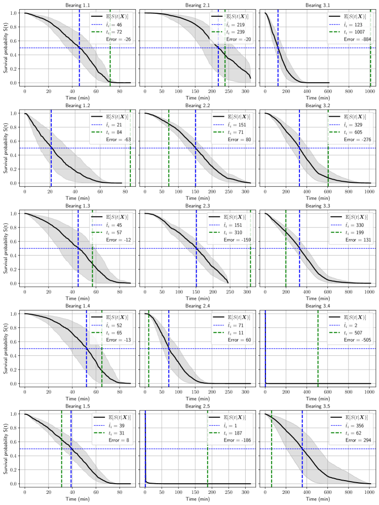
Figure 8: Predicted individual survival distribution (ISD) of each bearing using the BNNSurv model [38] (Blue line: predicted event time $\hat{t}_{i}$; Green line: actual event time $t_{i}$; Shaded grey: the region between the upper and lower bounds of a 90% credible interval). Bearings are separated by their operating condition (three columns) and index (five rows). The prediction error is the difference between the predicted time (the cross point of the vertical and horizontal blue lines) and the observed event time (green dash-dotted line).

5.6 Comparison to SOTA

We adopt the cumulative relative accuracy (CRA) metric to compare our approach to others [52]. This metric can fully assess the accuracy of a prognostic approach by aggregating the relative prediction accuracies at any inspection time. Given a RUL prediction, the CRA is:

$$CRA=K\sum_{k=1}^{K}w_{k}\,RA(T_{k}),$$ (7)

where $K$ is the number of inspection windows, $w_{k}$ is a normalized weight factor with $\frac{k}{\sum_{k=1}^{K}k}$ and $RA(T_{k})$ is the relative prediction accuracy at inspection time $T_{k}$:

$$RA(T_{k})=1-\frac{\left|\text{ActRUL}(T_{k})-\text{RUL}(T_{k})\right|}{\text{ActRUL}(T_{k})},$$ (8)

where ActRUL($T_{k}$) is the actual RUL at inspection time $T_{k}$, and RUL($T_{k}$) is the estimated RUL. The closer the CRA is to one, the more accurate the RUL estimation. Table 9 shows the results of the performance evaluation of the six methods, including our own framework using the RSF [29] model.

Unfortunately, none of the rival methods provided source code or a way to reproduce their results, so we reported the CRA as it was. For our method, we set the inspection time $T_{k}=1$ and use sensor data from the horizontal axis only as suggested by [62]. We see that our framework provides state-of-the-art predictive performance in terms of CRA for operating condition C1, but when we decrease the load and broaden the event horizon in C2 and C3, the predictions fluctuate a lot more and generally perform slightly worse than the state-of-the-art. We attribute this behavior to the variance in the XJTU-SY dataset, as some bearings have considerably different lifetimes, although they are run under the same operating condition (see Tab. 4). We also have notably fewer training samples at our disposal than many state-of-the-art works, since we estimate the RUL as the time to predictive maintenance, not the time to bearing failure. In some cases, this means that we only have a quarter of the training data available compared to the other methods (see Tab. 4).

We would have liked to compare our method with [66], who also adopted the XJTU-SY dataset and proposed a compelling two-stage prediction method, however, the authors only provided aggregated CRA results. Similarly, [71] proposed a multiscale encoder-decoder consisting of a convolutional neural network and a multihead attention mechanism, but the authors only provided a single root mean square error, not an individual RUL estimate. [57] proposed a deep adaptive transformer model, which supposedly provides better forecasting performance and solves the problem of vanishing gradients in existing recurrent architectures, but the reported relative accuracy is only for two of the fifteen bearings in the XJTU-SY dataset. Furthermore, the authors did not provide source code to reproduce their results.

Operating condition	Bearing dataset	RVM	DBN	PF	EKF	Hybrid	Our (RSF)
C1 (high)	Bearing 1_1	0.5741	0.4318	0.6107	0.6209	0.9047	0.8745
	Bearing 1_2	0.1815	0.6248	0.7256	0.3500	0.8546	0.5501
	Bearing 1_3	0.6245	0.5571	0.4850	0.8010	0.8482	0.8782
	Bearing 1_4	0.3722	-0.9479	0.2305	0.6839	0.7240	0.6922
	Bearing 1_5	0.6122	0.6636	0.4311	0.5042	0.7878	0.7980
C2 (medium)	Bearing 2_1	0.5718	0.5518	0.3963	0.5150	0.8621	0.7649
	Bearing 2_2	0.1789	-0.1977	0.2634	0.4314	0.6521	-0.7065
	Bearing 2_3	0.6172	0.9013	0.7364	0.8800	0.9612	0.4041
	Bearing 2_4	-0.0693	0.5316	0.4633	0.5004	0.6276	-8.3418
	Bearing 2_5	0.2563	0.0671	0.1833	0.4815	0.6328	0.0388
C3 (low)	Bearing 3_1	0.4329	0.6979	0.6557	0.7744	0.8942	0.1936
	Bearing 3_2	0.2225	-0.1301	0.1518	0.5362	0.6517	0.3039
	Bearing 3_3	-0.0883	0.5167	0.1283	-0.9653	0.8887	-0.5153
	Bearing 3_4	0.6570	0.6050	0.7830	0.6670	0.8133	0.6112
	Bearing 3_5	0.4881	0.5618	0.3857	0.5040	0.6512	-1.4658

Table 9: Cumulative relative accuracy (CRA) scores of six RUL estimation methods. This comparison includes relevance vector machines (RVM) [16], deep belief network (DBN) [74], particle filtering (PF) [36], extended Kalman filtering (EKF) [54], hybrid prognostics [62], and our framework using Random Survival Forests (RSF) [29].

6 Limitations and future work

6.1 Limitations

We propose an event detection algorithm based on the KL divergence. This offers interpretability, as opposed to using a deep learning architecture, but also requires manual feature engineering and fine-tuning, since we have to carefully select the frequency bands and calibrate the threshold function to avoid false positives and false negatives. In addition, there are some challenges in using the proposed frequency spectra to identify anomalies:

1. The fault frequency is based on the assumption that no sliding occurs between the rolling element and the bearing raceway, i.e., these rolling elements will only roll on the raceway. Under low load, this is rarely the case, as the rolling element often undergoes a combination of rolling and sliding movement if the load is insufficient to overcome the friction imposed by the lubricant. As a consequence, the calculated frequency may deviate from the real fault frequency and make this manually determined feature less informative of a bearing defect.

2. In all bearing applications and machines, the observed vibration signature will be a sum of contributions from mechanical components in the system; bearing defects, bearing looseness, misalignment of shafts from e.g. motor to gearbox, imbalance in rotating parts, gear-teeth meshing are examples of this. These contributions will interact, and the resultant characteristic frequencies can add or subtract, with a magnitude determined by the sensor location and how mobile each component is, obfuscating the informative frequencies.

3. Bearing preload and clearance will affect the eigenfrequencies of the rolling elements and as a result lead to changes in magnitude and a shift in the frequency bands that are excited during the overroling of infant bearing defects. Furthermore, changes in temperature can also lead to thermal expansion that affects the contact angle between the roller and the raceway, leading to volatile bearing frequencies.

4. Additional factors, such as the quality of lubrication, the roughness of the rolling element surface, and changes in surface conformance, do not manifest themselves as a characteristic cyclic frequency, which makes them very difficult to detect with traditional model-based spectral analysis or classical data-driven ML methods.

5. The sensitivity of various features that indicate a defect may vary considerably under different operating conditions. A very thorough and systematic learning stage is typically required to test the sensitivity of these frequencies under any desirable operating condition before they can actually be put into use with the traditional approach.

We adopted three survival models (CoxPH, CoxBoost and BNNSurv) that assume proportional hazards, which means the survival curves must have hazard functions that are proportional over time. Also, the change in the log-hazard rate associated with a particular covariate value is the same at all times. However, this assumption is easier to satisfy when the event horizon is short. In an industrial setting, where a bearing lasts longer than under artificially accelerated degradation, the event time distribution may have temporal dependencies at different time scales that are not easily captured by time invariant models that assume independence among data points. Thus, the proposed framework should be extended to consider time-varying covariates, i.e., by relaxing the proportional hazards assumption and allowing the hazard ratio to depend on time (see Sec. 6.2).

Based on the estimated survival probability, we take the median of the curve (0.5) as the predicted time to event. Other approaches have been proposed, such as calculating the Area Under the Curve (AUC), or simulating the survival times [5] based on some probability distribution. However, it is unlikely that a single bearing will fail at the exact time the survival curve reaches 0.5, but the average bearing will, given a large enough sample size. The XJTU-SY dataset only comes with five bearings per operating condition and there is pronounced variability between signals too, even for bearings that are tested under the same load configuration.

6.2 Future work

We find it appealing to test the proposed method on an industrial dataset to validate its practicality. The XJTU-SY dataset only comes with five bearings per operating condition and they have all been subjected to accelerated degradation, which substantially shortens their lifespan compared to actual industrial bearings. A real-world dataset would not have these characteristics. We also want to extend our framework to support time-varying covariates, thus incorporating temporal information between the vibration signals in the model. This can be done by replacing the learned representation with a recurrent neural network (RNN) architecture, such as a standard RNN or its variants, for example, GRU [12] or LSTM [23]. Three of the five proposed models assume proportional hazards, which is a reasonable assumption when working with artificially accelerated deterioration conditions. However, the proportional hazard assumption is unlikely to hold in an industrial setup. Thus, models that support time-varying covariates or models that do not rely on the proportional hazard assumption may be more suited for industrial application.

7 Conclusion

We have presented a novel, probabilistic, and interpretable framework for bearing diagnostics and RUL estimation using survival analysis. The proposed framework was shown to reliably detect the event of interest before the end of life, which facilitates timely predictive maintenance, and has several advantages over the Kaplan-Meier [67, 68] and CoxPH approaches [10, 65]: (1) It offers a covariate-based model with a probabilistic interpretation, supporting continuous and binary predictors. (2) It uses the median of the survival curve (0.5) as the event time, providing a quantitative and appropriate measure of the event occurrence, rivaling state-of-the-art performance in the XJTU-SY dataset. This approach contrasts with [68], who defined the time of the event as when the survival curve reached zero probability. (3) It can predict survival functions on a stratified set of covariates throughout the event horizon. (4) Adopting the Bayesian framework, our model can predict an individual survival distribution for each bearing with credible intervals, exhibiting the underlying uncertainty. This can improve the credibility of the prediction and make the framework more suitable as a decision-support tool. The Bayesian model was shown to be coverage calibrated; thus, its credible intervals matched the observed probability according to Pearson’s $\chi^{2}$ goodness-of-fit test.

CRediT authorship contribution statement

Christian Marius Lillelund: Conceptualization, Methodology, Writing - Original draft preparation, Software, Validation, Revision. Fernando Pannullo: Conceptualization, Methodology, Writing - Reviewing and Editing, Software, Revision. Morten Opprud Jakobsen: Data Curation, Conceptualization, Writing - Reviewing and Editing, Revision. Manuel Morante: Conceptualization, Methodology, Writing - Reviewing and Editing, Revision. Christian Fischer Pedersen: Conceptualization, Methodology, Supervision, Revision.

Declaration of competing interest

The authors declare that they have no known competing financial interests or personal relationships that could have appeared to influence the work reported in this paper.

Data availability

The XJTU-SY dataset is freely available. A download link can be found in the source code repository.

Appendix A Survival models

CoxPH [13]: The Cox proportional hazards model is a popular semiparametric method for fitting a regression model to survival data. Semiparametric models require no knowledge of the underlying distribution of the time to event, but the properties are assumed to have an exponential influence on the outcome. These models generally offer a more consistent estimator than parametric methods under a broader range of conditions and also a more precise estimator than nonparametric models [45]. The CoxPH model assumes a conditional individual hazard function of the form:

$$h\left(t|\bm{x}_{i}\right)=h_{0}\left(t\right)\exp\left(f\left(\bm{\theta},\bm{x}_{i}\right)\right)\text{,}$$ (9)

where $f\left(\bm{\theta},\bm{x}_{i}\right)$ denotes a risk score, and is a linear function of the covariates, i.e., $f\left(\bm{\theta},\bm{x}_{i}\right)=\bm{x}_{i}\bm{\theta}$, and the maximum likelihood estimator $\hat{\theta}$ is derived by numerically maximizing the partial log-likelihood:

$$\log p\left(\mathcal{D}|\bm{\theta}\right) =\sum_{i:\delta_{i}=1}\log\frac{h\left(y_{i}|\bm{x}_{i}\right)}{\sum_{j:T_{j}\geq T_{i}}h\left(y_{i}|\bm{x}_{j}\right)}\text{,}$$

$$=\sum_{i:\delta_{i}=1}f\left(\bm{\theta},\bm{x}_{i}\right)-\sum_{j:T_{j}\geq T_{i}}f\left(\bm{\theta},\bm{x}_{j}\right)\text{.}$$ (10)

CoxBoost [8]: The CoxBoost method adopts a gradient boosting approach [20] to estimate parameters $\bm{\theta}$ by maximising Eq. A as in the CoxPH model and considers a flexible set of candidate covariates. In each boosting step, there are $q_{k}$ predetermined candidates sets of covariates, and for each of these $q_{k}$ sets, it simultaneously updates the parameter for the corresponding covariate. Regular gradient boosting would update only one component of $\bm{\theta}$ in component-wise boosting, or fit the gradient by using all covariates in each step.

RSF [29]: The Random Survival Forests model is an extension of regular decision trees for survival analysis, which are made to handle censored data. During training, data are recursively partitioned based on some splitting criterion, and similar data points based on the event of interest are put on the same node. This ensures a decorrelation of individual trees by iteratively building each tree on a different bootstrap sample of the original training data and then at each node only evaluate the split criterion for a randomly selected subset of features and thresholds. Predictions are then formed by aggregating predictions of individual trees in the ensemble, like a regular Random Forests.

MTLR [72]: Multi-task logistic regression directly models the individual survival function by combining multiple local logistic regression models. It discretizes the event horizon into $K$ bins $(\tau_{0}=0,\tau_{1}),(\tau_{1},\tau_{2}),\ldots,(\tau_{K-1},\tau_{K})$ and computes the probability of event at each bin by fitting a logistic regression model [47]. The predicted event time $\hat{t_{i}}$ can be then be encoded deterministically using a $K$-dimensional binary sequence $\mathbf{y}_{i}=(y_{i,1},y_{i,2},\ldots,y_{i,K})\in\mathbb{Z}^{K}$ where $y_{i,k}=0$ means that the observation had not experienced the event at time $\tau_{k-1}$, and $y_{i,k}=1$ means the observation experienced the event before time $\tau_{k-1}$ [47]. Unlike the CoxPH model, MTLR does not impose the proportional assumption on the hazard function, nor does it assume that the survival function follows a specific distribution.

BNNSurv [38]: BNNSurv is a Bayesian Neural Network for survival analysis. Similar to DeepSurv, it uses the Cox partial log-likehood to optimize the objective Eq. (A), but the weights and biases of the network are treated as random variables with an unknown posterior distribution. During training, they are estimated with an approximate distribution using, e.g., variational inference (VI), Monte Carlo dropout (MCD), or another inference technique. The output nodes thus provide the mean and standard deviation of a risk score, $\hat{r}_{i}$, as Gaussian samples, that is, $\hat{r}_{i}\sim\mathcal{N}\left(\mu_{\bm{x}_{i}},\sigma_{\bm{x}_{i}}\right)$ for a $d$-dimensional sample $\bm{x}_{i}$. In this work, we adopt BNNSurv using MCD inference and set a dropout rate of 25%.

Appendix B Performance metrics

MAE: The mean absolute error is the absolute difference between the actual and predicted survival times (defined as the median time of the predicted survival curve). Given an individual survival distribution (ISD), $S\left(t\;|\;\bm{x}_{i}\right)=\text{P}\left(T>t\;|\;\bm{X}=\bm{x}_{i}\right)$, we compute the predicted survival time $\hat{t}_{i}$ as the median survival time [46]:

$$\hat{t}_{i}=\text{median}\;(S(t\;|\;\bm{x}_{i}))=S^{-1}(\tau=0.5\;|\;\bm{x}_{i})\text{,}$$ (11)

where $\tau\in[0,1]$ represents the quantile probability level. Given $\hat{t}_{i}$ and ${t}_{i}$, it is then trivial to calculate the MAE if the event is observed ($\delta_{i}=1$) [46]:

$$\text{MAE}\;(\hat{t}_{i},t_{i},\delta_{i}=1)=|\;t_{i}-\hat{t}_{i}\;|\text{.}$$ (12)

MAE_H: In cases where the event is not observed ($\delta_{i}=0$), there are still ways to calculate the MAE. One example is using a Hinge loss function accommodating the censored observations: if the predicted survival time $\hat{t_{i}}$ is less than the censoring time $c_{i}$, the loss equals the censoring time minus the predicted time. When the predicted survival time is equal to or exceeds the censoring time, the loss is zero [46]:

$$\text{MAE-Hinge}\;(\hat{t}_{i},t_{i},\delta_{i}=0)=\text{max}\;\left(t_{i}-\hat{t}_{i},\;0\right)\text{.}$$ (13)

MAE_M: Another way to accommodate censored observations is by assigning a “best guess” value (margin time) to each censored observation [26], using the Kaplan-Meier (KM) estimator [32]. Given the event time $e_{j}$ is greater than the censoring time $c_{i}$, the margin time is then a conditional expectation of the event time given some observation censored at $t_{i}$ [46]:

$$e_{\text{margin}}(t_{i},D)=\mathbb{E}_{t}[e_{i}\,|\,e_{i}>t_{i}]=t_{i}+\frac{\int_{t_{i}}^{\infty}t\,S_{\text{KM}}(D)(t)\,dt}{S_{\text{KM}}(D)(t)}\text{,}$$ (14)

where $S_{\text{KM}}(D)(t)$ in the KM estimator derived from the training data. [26] proposed using a confidence weight $\omega_{i}=1-S_{\text{KM}}(D)(t_{i})$ based on the margin value, which gives lower confidence for observations censored early and higher confidence for observations censored late ($\omega=1$ for uncensored observations). Adopting this weighting scheme, the MAE-margin is then [46]:

$$\text{MAE-Margin}(\hat{t}_{i},t_{i},\delta_{i})]$$

$$=\frac{1}{\sum_{i=1}^{N}\omega_{i}}\sum_{i=1}^{N}\omega_{i}\cdot|[(1-\delta_{i})\cdot e_{\text{margin}}(t_{i})+\delta_{i}\cdot t_{i}]-\hat{t}_{i}|\text{.}$$ (15)

MAE_PO: We can also substitute the unobserved event times with pseudo-observations [3, 4]. Let $\{t_{i}\}_{i=1}^{N}$ be i.i.d. draws of a random variable time, $T$, and let $\hat{\theta}$ be an unbiased estimator for the event time based on right-censored observations of $T$. The pseudo-observation for a censored subject is defined as:

$$e_{\text{pseudo}}(t_{i},D)=N\times\hat{\theta}-(N-1)\times\hat{\theta}^{-i}\text{,}$$ (16)

where $\hat{\theta}^{-i}$ is the estimator applied to the $N-1$ element dataset formed by removing that $i$-th observation. The pseudo-observation can be viewed as the contribution of subject $i$ to the unbiased event time estimation $\hat{\theta}$. Following [46], we estimate $\hat{\theta}$ using the KM estimator, i.e., $\hat{\theta}=E_{t}[S_{\text{KM}}(D)(t)]$ and $\hat{\theta}^{-i}=E_{t}[S_{\text{KM}}(D^{-i})(t)]$ as unbiased estimators. After calculating the pseudo-observation values using Eq. 16, MAE-pseudo-observation (MAE_PO) can be calculated using the weighting scheme in Eq. B.

D-Calibration: Distribution calibration assesses the calibration performance of the survival curve $S(t)$ [26], informing us to which extent we should trust the predicted probabilities. For each uncensored observation $\bm{x}_{i}$ with observed event time $y_{i}$, we determine the probability $P(S(t\text{\textbar}\bm{x}{i}(t))$ for that time based on $S(t)$. Following the example of [26], if $S(t)$ is D-Calibrated, we anticipate 10% of the events to fall in the [90%, 100%] interval and another 10% to fall in the [80%, 90%] interval. For all individual distributions $d_{i}$, the set $\{S_{i}(d_{i})\}$ should exhibit a uniform distribution between zero and one, ensuring each 10%-interval covers 10% of $D$. We use Pearson’s $\chi^{2}$ goodness-of-fit test, checking if the proportion of events in each interval is uniformly distributed within mutually exclusive and equal-sized intervals, as proposed by [26].

C-Calibration: Coverage calibration is a test to assess the alignment between the predicted credible intervals (CrIs) and observed probability intervals [47], i.e., a p% probability CrI should give individual CrIs with a probability of p% to encompass an individual’s likelihood of event. The coverage calibration procedure involves calculating observed coverage rates using CrIs with varying percentages (ranging from 10% to 90%). We follow the approach by [47] and use a Pearson’s $\chi^{2}$ test to evaluate the calibration of the observed and expected coverage rates. The null hypothesis is that the observed coverages are consistent across all percentage rate groups. Models that show similarity between expected and observed event rates in subgroups are C-calibrated. This test is specific for the BNNSurv model [38].

References

- Al Masry et al. [2019] Al Masry, Z., Schaible, P., Zerhouni, N., Varnier, C., 2019. Remaining useful life prediction for ball bearings based on health indicators. MATEC Web of Conferences 261, 02003. doi:10.1051/matecconf/201926102003.
- An et al. [2019] An, Z., Li, S., Wang, J., Xin, Y., Xu, K., 2019. Generalization of deep neural network for bearing fault diagnosis under different working conditions using multiple kernel method. Neurocomputing 352, 42–53. doi:https://doi.org/10.1016/j.neucom.2019.04.010.
- Andersen et al. [2003] Andersen, P.K., Klein, J.P., Rosthøj, S., 2003. Generalised linear models for correlated pseudo‐observations, with applications to multi‐state models. Biometrika 90, 15–27. doi:10.1093/biomet/90.1.15.
- Andersen and Perme [2010] Andersen, P.K., Perme, M.P., 2010. Pseudo-observations in survival analysis. Statistical Methods in Medical Research 19, 71–99. doi:10.1177/0962280209105020.
- Austin [2012] Austin, P.C., 2012. Generating survival times to simulate cox proportional hazards models with time-varying covariates. Statistics in Medicine 31, 3946–3958. doi:https://doi.org/10.1002/sim.5452.
- Awadallah and Morcos [2003] Awadallah, M., Morcos, M., 2003. Application of ai tools in fault diagnosis of electrical machines and drives-an overview. IEEE Transactions on Energy Conversion 18, 245–251. doi:https://doi.org/10.1109/TEC.2003.811739.
- Batista et al. [2013] Batista, L., Badri, B., Sabourin, R., Thomas, M., 2013. A classifier fusion system for bearing fault diagnosis. Expert Systems with Applications 40, 6788–6797. doi:https://doi.org/10.1016/j.eswa.2013.06.033.
- Binder and Schumacher [2008] Binder, H., Schumacher, M., 2008. Allowing for mandatory covariates in boosting estimation of sparse high-dimensional survival models. BMC Bioinformatics 9, 14. doi:10.1186/1471-2105-9-14.
- Cerrada et al. [2018] Cerrada, M., Sánchez, R.V., Li, C., Pacheco, F., Cabrera, D., Valente de Oliveira, J., Vásquez, R.E., 2018. A review on data-driven fault severity assessment in rolling bearings. Mechanical Systems and Signal Processing 99, 169–196. doi:https://doi.org/10.1016/j.ymssp.2017.06.012.
- Chen et al. [2020] Chen, C., Liu, Y., Wang, S., Sun, X., Di Cairano-Gilfedder, C., Titmus, S., Syntetos, A.A., 2020. Predictive maintenance using cox proportional hazard deep learning. Advanced Engineering Informatics 44, 101054. doi:https://doi.org/10.1016/j.aei.2020.101054.
- Cheng et al. [2021] Cheng, Y., Hu, K., Wu, J., Zhu, H., Shao, X., 2021. A convolutional neural network based degradation indicator construction and health prognosis using bidirectional long short-term memory network for rolling bearings. Advanced Engineering Informatics 48, 101247. doi:https://doi.org/10.1016/j.aei.2021.101247.
- Cho et al. [2014] Cho, K., van Merriënboer, B., Bahdanau, D., Bengio, Y., 2014. On the properties of neural machine translation: Encoder–decoder approaches, in: Proceedings of SSST-8, Eighth Workshop on Syntax, Semantics and Structure in Statistical Translation, pp. 103–111. doi:10.3115/v1/W14-4012.
- Cox [1972] Cox, D.R., 1972. Regression Models and Life-Tables. Journal of the Royal Statistical Society 34, 187–202.
- Cubillo et al. [2016] Cubillo, A., Perinpanayagam, S., Esperon-Miguez, M., 2016. A review of physics-based models in prognostics: Application to gears and bearings of rotating machinery. Advances in Mechanical Engineering 8, 1687814016664660. doi:https://doi.org/10.1177/1687814016664660.
- Delpha et al. [2017] Delpha, C., Diallo, D., Youssef, A., 2017. Kullback-leibler divergence for fault estimation and isolation : Application to gamma distributed data. Mechanical Systems and Signal Processing 93, 118–135. doi:https://doi.org/10.1016/j.ymssp.2017.01.045.
- Di Maio et al. [2012] Di Maio, F., Tsui, K.L., Zio, E., 2012. Combining relevance vector machines and exponential regression for bearing residual life estimation. Mechanical Systems and Signal Processing 31, 405–427. doi:https://doi.org/10.1016/j.ymssp.2012.03.011.
- Dong and Luo [2013] Dong, S., Luo, T., 2013. Bearing degradation process prediction based on the pca and optimized ls-svm model. Measurement 46, 3143–3152. doi:https://doi.org/10.1016/j.measurement.2013.06.038.
- Ferreira and Gonçalves [2022] Ferreira, C., Gonçalves, G., 2022. Remaining Useful Life prediction and challenges: A literature review on the use of Machine Learning Methods. Journal of Manufacturing Systems 63, 550–562.
- Filippetti et al. [2000] Filippetti, F., Franceschini, G., Tassoni, C., Vas, P., 2000. Recent developments of induction motor drives fault diagnosis using ai techniques. IEEE Transactions on Industrial Electronics 47, 994–1004. doi:https://doi.org/10.1109/41.873207.
- Friedman [2001] Friedman, J.H., 2001. Greedy Function Approximation: A Gradient Boosting Machine. The Annals of Statistics 29, 1189–1232. doi:10.1214/aos/1013203451.
- Gal and Ghahramani [2016] Gal, Y., Ghahramani, Z., 2016. Dropout as a bayesian approximation: Representing model uncertainty in deep learning, in: Proceedings of The 33rd International Conference on Machine Learning, pp. 1050–1059.
- Gareth et al. [2021] Gareth, J., Daniela, W., Trevor, H., Robert, T., 2021. An introduction to statistical learning: with applications in R. 2 ed., Spinger.
- Gers et al. [1999] Gers, F., Schmidhuber, J., Cummins, F., 1999. Learning to forget: continual prediction with lstm, in: 1999 Ninth International Conference on Artificial Neural Networks ICANN 99. (Conf. Publ. No. 470), pp. 850–855. doi:https://doi.org/10.1049/cp:19991218.
- Goodfellow et al. [2016] Goodfellow, I.J., Bengio, Y., Courville, A., 2016. Deep Learning. MIT Press.
- Guo et al. [2017] Guo, L., Li, N., Jia, F., Lei, Y., Lin, J., 2017. A recurrent neural network based health indicator for remaining useful life prediction of bearings. Neurocomputing 240, 98–109. doi:https://doi.org/10.1016/j.neucom.2017.02.045.
- Haider et al. [2020] Haider, H., Hoehn, B., Davis, S., Greiner, R., 2020. Effective ways to build and evaluate individual survival distributions. Journal of Machine Learning Research 21, 1–63.
- Hochstein et al. [2013] Hochstein, A., Ahn, H.I., Leung, Y.T., Denesuk, M., 2013. Survival analysis for HDLSS data with time dependent variables: Lessons from predictive maintenance at a mining service provider, in: Proceedings of 2013 IEEE International Conference on Service Operations and Logistics, and Informatics, pp. 372–381. doi:https://doi.org/10.1109/SOLI.2013.6611443.
- Huang et al. [2007] Huang, R., Xi, L., Li, X., Richard Liu, C., Qiu, H., Lee, J., 2007. Residual life predictions for ball bearings based on self-organizing map and back propagation neural network methods. Mechanical Systems and Signal Processing 21, 193–207. doi:https://doi.org/10.1016/j.ymssp.2005.11.008.
- Ishwaran et al. [2008] Ishwaran, H., Kogalur, U.B., Blackstone, E.H., Lauer, M.S., 2008. Random Survival Forests. The Annals of Applied Statistics 2, 841–860. doi:https://doi.org/10.1214/08-AOAS169.
- ISO [2007] ISO, 2007. Rolling Bearings - Dynamic Load rating and rating life.
- Jia et al. [2018] Jia, F., Lei, Y., Guo, L., Lin, J., Xing, S., 2018. A neural network constructed by deep learning technique and its application to intelligent fault diagnosis of machines. Neurocomputing 272, 619–628. doi:https://doi.org/10.1016/j.neucom.2017.07.032.
- Kaplan and Meier [1958] Kaplan, E.L., Meier, P., 1958. Nonparametric Estimation from Incomplete Observations. Journal of the American Statistical Association 53, 457–481. doi:10.2307/2281868.
- Kim et al. [2019] Kim, D.W., Lee, S., Kwon, S., Nam, W., Cha, I.H., Kim, H.J., 2019. Deep learning-based survival prediction of oral cancer patients. Scientific Reports 9, 6994. doi:https://doi.org/10.1038/s41598-019-43372-7.
- Kim et al. [2017] Kim, N.H., An, D., Choi, J.H., 2017. Prognostics and Health Management of Engineering Systems. Springer International Publishing.
- Kullback and Leibler [1951] Kullback, S., Leibler, R.A., 1951. On information and sufficiency. The annals of mathematical statistics 22, 79–86.
- Liao [2014] Liao, L., 2014. Discovering prognostic features using genetic programming in remaining useful life prediction. IEEE Transactions on Industrial Electronics 61, 2464–2472. doi:https://doi.org/10.1109/TIE.2013.2270212.
- Liewald et al. [2022] Liewald, M., Bergs, T., Groche, P., Behrens, B.A., Briesenick, D., Müller, M., Niemietz, P., Kubik, C., Müller, F., 2022. Perspectives on data-driven models and its potentials in metal forming and blanking technologies. Production Engineering 16, 607–625. doi:https://doi.org/10.1007/s11740-022-01115-0.
- Lillelund et al. [2023a] Lillelund, C.M., Magris, M., Pedersen, C.F., 2023a. Uncertainty estimation in deep bayesian survival models, in: 2023 IEEE EMBS International Conference on Biomedical and Health Informatics (BHI), pp. 1–4. doi:https://doi.org/10.1109/BHI58575.2023.10313466.
- Lillelund et al. [2023b] Lillelund, C.M., Pannullo, F., Jakobsen, M.O., Pedersen, C.F., 2023b. Predicting survival time of ball bearings in the presence of censoring. Accepted at AAAI Fall Symposium 2023 on Survival Prediction. arXiv:2309.07188.
- Liu et al. [2018] Liu, R., Yang, B., Zio, E., Chen, X., 2018. Artificial intelligence for fault diagnosis of rotating machinery: A review. Mechanical Systems and Signal Processing 108, 33–47. doi:https://doi.org/10.1016/j.ymssp.2018.02.016.
- Magris and Iosifidis [2023] Magris, M., Iosifidis, A., 2023. Bayesian learning for neural networks: an algorithmic survey. Artificial Intelligence Review , 1–51.
- Montavon et al. [2018] Montavon, G., Samek, W., Müller, K.R., 2018. Methods for interpreting and understanding deep neural networks. Digital Signal Processing 73, 1–15. doi:https://doi.org/10.1016/j.dsp.2017.10.011.
- Nagpal et al. [2021] Nagpal, C., Li, X., Dubrawski, A., 2021. Deep survival machines: Fully parametric survival regression and representation learning for censored data with competing risks. IEEE Journal of Biomedical and Health Informatics 25, 3163–3175. doi:https://doi.org/10.1109/JBHI.2021.3052441.
- Peng et al. [2020] Peng, W., Ye, Z.S., Chen, N., 2020. Bayesian deep-learning-based health prognostics toward prognostics uncertainty. IEEE Transactions on Industrial Electronics 67, 2283–2293. doi:https://doi.org/10.1109/TIE.2019.2907440.
- Powell [1994] Powell, J.L., 1994. Chapter 41 estimation of semiparametric models, in: Handbook of Econometrics. volume 4, pp. 2443–2521. doi:https://doi.org/10.1016/S1573-4412(05)80010-8.
- Qi et al. [2023a] Qi, S., Kumar, N., Farrokh, M., Sun, W., Kuan, L., Ranganath, R., Henao, R., Greiner, R., 2023a. An effective meaningful way to evaluate survival models. Proceedings of Machine Learning Research 202, 28244–28276.
- Qi et al. [2023b] Qi, S.a., Kumar, N., Verma, R., Xu, J.Y., Shen-Tu, G., Greiner, R., 2023b. Using bayesian neural networks to select features and compute credible intervals for personalized survival prediction. IEEE Transactions on Biomedical Engineering 70, 3389–3400. doi:https://doi.org/10.1109/TBME.2023.3287514.
- Qin et al. [2021] Qin, A.S., Mao, H.L., Hu, Q., 2021. Cross-domain fault diagnosis of rolling bearing using similar features-based transfer approach. Measurement 172, 108900. doi:https://doi.org/10.1016/j.measurement.2020.108900.
- Qiu et al. [2006] Qiu, H., Lee, J., Lin, J., Yu, G., 2006. Wavelet filter-based weak signature detection method and its application on rolling element bearing prognostics. Journal of Sound and Vibration 289, 1066–1090. doi:https://doi.org/10.1016/j.jsv.2005.03.007.
- Randall [2021] Randall, R.B., 2021. Vibration–based Condition Monitoring: Industrial, Automotive and Aerospace Applications. 2 ed., John Wiley & Sons, Ltd.
- Randall and Antoni [2011] Randall, R.B., Antoni, J., 2011. Rolling element bearing diagnostics—a tutorial. Mechanical Systems and Signal Processing 25, 485–520. doi:https://doi.org/10.1016/j.ymssp.2010.07.017.
- Saxena et al. [2021] Saxena, A., Celaya, J., Saha, B., Saha, S., Goebel, K., 2021. Metrics for Offline Evaluation of Prognostic Performance. International Journal of Prognostics and Health Management 1. doi:https://doi.org/10.36001/ijphm.2010.v1i1.1336.
- Shenfield and Howarth [2020] Shenfield, A., Howarth, M., 2020. A novel deep learning model for the detection and identification of rolling element-bearing faults. Sensors 20. doi:https://doi.org/10.3390/s20185112.
- Singleton et al. [2015] Singleton, R.K., Strangas, E.G., Aviyente, S., 2015. Extended kalman filtering for remaining-useful-life estimation of bearings. IEEE Transactions on Industrial Electronics 62, 1781–1790. doi:https://doi.org/10.1109/TIE.2014.2336616.
- SKF [2017] SKF, 2017. Bearing damage and failure analysis. Technical Report. SKF. URL: https://cdn.skfmediahub.skf.com/api/public/0901d1968064c148/pdf_preview_medium/0901d1968064c148_pdf_preview_medium.pdf.
- Stepanova and Thomas [2002] Stepanova, M., Thomas, L., 2002. Survival Analysis Methods for Personal Loan Data. Operations Research 50, 277–289.
- Su et al. [2021] Su, X., Liu, H., Tao, L., Lu, C., Suo, M., 2021. An end-to-end framework for remaining useful life prediction of rolling bearing based on feature pre-extraction mechanism and deep adaptive transformer model. Computers & Industrial Engineering 161, 107531. doi:https://doi.org/10.1016/j.cie.2021.107531.
- Tabatabaei et al. [2020] Tabatabaei, R., Aasi, A., Jafari, S.M., Ciulli, E., 2020. Experimental Investigation of the Diagnosis of Angular Contact Ball Bearings Using Acoustic Emission Method and Empirical Mode Decomposition. Advances in Tribology 2020, 1–14. doi:https://doi.org/10.1155/2020/8231752.
- Theodoridis [2020] Theodoridis, S., 2020. Machine Learning: A Bayesian and Optimization Perspective. 2 ed., Elsevier Science.
- Tian et al. [2015] Tian, Y., Ma, J., Lu, C., Wang, Z., 2015. Rolling bearing fault diagnosis under variable conditions using lmd-svd and extreme learning machine. Mechanism and Machine Theory 90, 175–186. doi:https://doi.org/10.1016/j.mechmachtheory.2015.03.014.
- Tobon-Mejia et al. [2012] Tobon-Mejia, D.A., Medjaher, K., Zerhouni, N., Tripot, G., 2012. A data-driven failure prognostics method based on mixture of gaussians hidden markov models. IEEE Transactions on Reliability 61, 491–503. doi:https://doi.org/10.1109/TR.2012.2194177.
- Wang et al. [2020] Wang, B., Lei, Y., Li, N., Li, N., 2020. A hybrid prognostics approach for estimating remaining useful life of rolling element bearings. IEEE Transactions on Reliability 69, 401–412. doi:https://doi.org/10.1109/TR.2018.2882682.
- Wang et al. [2017] Wang, J., Li, C., Han, S., Sarkar, S., Zhou, X., 2017. Predictive maintenance based on event-log analysis: A case study. IBM Journal of Research and Development 61, 11:121–11:132. doi:https://doi.org/10.1147/JRD.2017.2648298.
- Wang et al. [2021] Wang, R., Chen, H., Guan, C., 2021. A bayesian inference-based approach for performance prognostics towards uncertainty quantification and its applications on the marine diesel engine. ISA Transactions 118, 159–173. doi:https://doi.org/10.1016/j.isatra.2021.02.024.
- Wang et al. [2022] Wang, Y., Zhao, J., Yang, C., Xu, D., Ge, J., 2022. Remaining useful life prediction of rolling bearings based on pearson correlation-kpca multi-feature fusion. Measurement 201, 111572. doi:https://doi.org/10.1016/j.measurement.2022.111572.
- Wang et al. [2023] Wang, Z., Ta, Y., Cai, W., Li, Y., 2023. Research on a remaining useful life prediction method for degradation angle identification two-stage degradation process. Mechanical Systems and Signal Processing 184, 109747. doi:https://doi.org/10.1016/j.ymssp.2022.109747.
- Widodo and Yang [2011a] Widodo, A., Yang, B.S., 2011a. Application of relevance vector machine and survival probability to machine degradation assessment. Expert Systems with Applications 38, 2592–2599. doi:https://doi.org/10.1016/j.eswa.2010.08.049.
- Widodo and Yang [2011b] Widodo, A., Yang, B.S., 2011b. Machine health prognostics using survival probability and support vector machine. Expert Systems with Applications 38, 8430–8437. doi:https://doi.org/10.1016/j.eswa.2011.01.038.
- Wu et al. [2023] Wu, Y., Liu, X., Wang, Y.L., Li, Q., Guo, Z., Jiang, Y., 2023. Improved deep pca and kullback–leibler divergence based incipient fault detection and isolation of high-speed railway traction devices. Sustainable Energy Technologies and Assessments 57, 103208. doi:https://doi.org/10.1016/j.seta.2023.103208.
- Xu et al. [2022] Xu, W., Jiang, Q., Shen, Y., Xu, F., Zhu, Q., 2022. Rul prediction for rolling bearings based on convolutional autoencoder and status degradation model. Applied Soft Computing 130, 109686. doi:https://doi.org/10.1016/j.asoc.2022.109686.
- Xu et al. [2023] Xu, Z., Bashir, M., Liu, Q., Miao, Z., Wang, X., Wang, J., Ekere, N., 2023. A novel health indicator for intelligent prediction of rolling bearing remaining useful life based on unsupervised learning model. Computers & Industrial Engineering 176, 108999. doi:https://doi.org/10.1016/j.cie.2023.108999.
- Yu et al. [2011] Yu, C.N., Greiner, R., Lin, H.C., Baracos, V., 2011. Learning patient-specific cancer survival distributions as a sequence of dependent regressors, in: Advances in Neural Information Processing Systems, pp. 1845––1853.
- Zeng et al. [2014] Zeng, J., Kruger, U., Geluk, J., Wang, X., Xie, L., 2014. Detecting abnormal situations using the kullback–leibler divergence. Automatica 50, 2777–2786. doi:https://doi.org/10.1016/j.automatica.2014.09.005.
- Zhang et al. [2017] Zhang, C., Lim, P., Qin, A.K., Tan, K.C., 2017. Multiobjective deep belief networks ensemble for remaining useful life estimation in prognostics. IEEE Transactions on Neural Networks and Learning Systems 28, 2306–2318. doi:https://doi.org/10.1109/TNNLS.2016.2582798.
- Zhang et al. [2011] Zhang, P., Du, Y., Habetler, T.G., Lu, B., 2011. A survey of condition monitoring and protection methods for medium-voltage induction motors. IEEE Transactions on Industry Applications 47, 34–46. doi:https://doi.org/10.1109/TIA.2010.2090839.
- Zheng et al. [2018] Zheng, C., Liu, W., Chen, B., Gao, D., Cheng, Y., Yang, Y., Zhang, X., Li, S., Huang, Z., Peng, J., 2018. A data-driven approach for remaining useful life prediction of aircraft engines, in: 2018 21st International Conference on Intelligent Transportation Systems (ITSC), pp. 184–189. doi:https://doi.org/10.1109/ITSC.2018.8569915.
- Zhu et al. [2016] Zhu, X., Yao, J., Huang, J., 2016. Deep convolutional neural network for survival analysis with pathological images, in: 2016 IEEE International Conference on Bioinformatics and Biomedicine (BIBM), pp. 544–547. doi:https://doi.org/10.1109/BIBM.2016.7822579.