Improving Trainability of Variational Quantum Circuits via Regularization Strategies

Abstract

In the era of noisy intermediate-scale quantum (NISQ), variational quantum circuits (VQCs) have been widely applied in various domains, advancing the superiority of quantum circuits against classic models. Similar to classic models, regular VQCs can be optimized by various gradient-based methods. However, the optimization may be initially trapped in barren plateaus or eventually entangled in saddle points during training. These gradient issues can significantly undermine the trainability of VQC. In this work, we propose a strategy that regularizes model parameters with prior knowledge of the train data and Gaussian noise diffusion. We conduct ablation studies to verify the effectiveness of our strategy across four public datasets and demonstrate that our method can improve the trainability of VQCs against the above-mentioned gradient issues.

I Introduction

In recent years, there have been significant advancements in quantum information, particularly with the advent of noisy intermediate-scale quantum (NISQ) devices [1]. Within this research landscape, variational quantum circuits (VQCs) have been widely applied in various domains, such as quantum machine learning [2], quantum physics [3, 4], and quantum hardware architecture [5, 6]. Typical VQCs are trainable random parameterized quantum circuits or classic-quantum hybrid models [7]. Similar to classic models, VQCs can be optimized by various gradient-based approaches, such as Adam [8]. However, optimization processes may encounter some gradient issues. Primarily, the initialization of VQCs might be trapped on a barren plateau landscape. McClean et al. [9] first systematically study the barren plateau (BP) issues and verify that the gradient variance will exponentially decrease as the model size increases when the VQCs satisfy the assumption of the 2-design Haar distribution. Under this circumstance, most gradient-based approaches would fail. Additionally, the optimization may be entangled in saddle points during training [10, 11]. Both gradient issues can significantly weaken the trainability of VQCs.

Extensive research has been devoted to solving the barren plateau problem, where initialization-based strategies have proven to be very effective by initializing VQC parameters with diverse distributions [12]. For instance, Zhang et al. [13] verify the effectiveness of Gaussian initialization on VQCs with a well-designed variance. Nevertheless, most initialization strategies neglect the impact of real data distribution. To address this oversight, Prince argues that applying the data posterior to model parameters could provide more robust performance [14]. However, posterior estimation on complex models may not be practical due to high computational overhead. To overcome the above drawbacks, we leverage prior knowledge of the train data to regularize the initial distribution of model parameters. Our intuition for this regularization is that applying prior knowledge in initialization can shape the initial distribution to some extent, thus promoting the alleviation of barren plateau issues.

Besides mitigating barren plateau issues via initialization-based strategies, some studies improve the trainability by adding noise to model parameters to avoid being trapped in saddle points during training  [15]. However, adding excessive noise may potentially undermine model performance [16]. Inspired by DDPM [17], which models the data distribution by iteratively diffusing Gaussian noise during data generation, we gradually diffuse Gaussian noise on model parameters during training. The intuition behind noise diffusion is that as training converges, the model will gradually perform better, thus requiring slighter noise perturbations on model parameters.

By integrating the above two mechanisms, in this study, we propose a regularization strategy to improve the trainability of VQCs. In our proposed method, we first leverage prior knowledge of the train data to regularize the initial distribution of model parameters, and further diffuse Gaussian noise on the parameters along each training iteration. In experiments, we conduct ablation studies to examine the effectiveness of our proposed methods. First, We validate that leveraging prior knowledge of the train data can effectively regularize eight prevalent initial distributions of model parameters and yield superior mitigation on barren plateau issues. Furthermore, we affirm that diffusing Gaussian noise to model parameters during training can efficaciously increase volatility to avoid being trapped in saddle points while adequately alleviating the degradation of gradient variance on five Gaussian-based strategies. Last, we analyze the key hyperparameter, max diffusion rate ($dr_{max}$), on Normal distribution as an example. Extensive results demonstrate the effectiveness of our proposed regularization strategy over four public datasets. Overall, our contributions to this study can be summarized as follows:

• We propose a strategy that regularizes model parameters with prior knowledge and Gaussian noise diffusion for improving the trainability of VQCs.

• We conduct extensive experiments to verify the effectiveness of our proposed method across four public datasets.

II Related Work

McClean et al. [9] first investigated barren plateau (BP) phenomenons and demonstrated that under the assumption of the 2-design Haar distribution, gradient variance in VQCs will exponentially decrease to zero during training as the model size increases. In recent years, enormous studies have been devoted to mitigating barren plateau issues in VQCs. In this study, we categorize these studies as initialization-based strategies [18], optimization-based strategies [19], model-based strategies [20], and measurement-based strategies [21]. First, initialization-based strategies mainly aim to initialize model parameters with different distributions. Within this category, Grant et al. [22] propose an identity block strategy that can initialize the VQCs as a sequence of blocks of identity operator. Sauvage et al. [23] propose a flexible initializer (FLIP) for arbitrarily sized VQCs. Kulshrestha et al. [15] initialize the circuit parameters from a beta distribution. Zhang et al. [13] verify that applying Gaussian initialization with well-designed variance can mitigate barren plateau issues. Second, optimization-based strategies primarily improve the efficiency of optimization while mitigating barren plateaus as well. For example, Ostaszewski et al. [24] propose a new method for effectively optimizing VQCs’ structure and parameters with lower computational overhead. Suzuki et al. [25] propose a new normalized gradient descent (NGD) method that can converge faster than the naive NGD-based method. Heyraud et al. [26] design an efficient method to compute the gradient for a wide range of VQCs. Third, model-based strategies address barren plateau problems via various model architectures. For example, Li et al. [7] propose a hybrid quantum-classical framework, namely VSQL, to avoid barren plateaus. Concurrently, Bharti and Haug [27] propose a hybrid quantum-classical algorithm for dynamically simulating quantum circuits. Du et al. [28] design an efficient search scheme, QAS, to automatically seek a near-optimum during VQCs’ training. Tüysüz et al. [29] propose a model to divide the VQCs into multiple sub-circuits to avoid barren plateaus. Kashif et al. [30] introduce residual quantum neural networks (ResQNets) by splitting QNN architectures into multiple quantum nodes. Last but not least, measurement-based strategies investigate the barren plateau landscape in hybrid variational quantum circuits from the perspective of measurement [21].

III Methodology

III-A Preliminary

Variational Quantum Circuits

Typical VQCs consist of a finite sequence of unitary gates $U(\theta)$ parameterized by $\theta\in\mathbb{R}^{NRL}$, where $N$, $R$, and $L$ denote the number of qubits, rotation gates, and layers. $U(\theta)$ can be formulated as:

$$U(\theta)=U(\theta_{1},...,\theta_{L})=\prod_{l=1}^{L}U_{l}(\theta_{l})W_{l},$$ (1)

where $U_{l}(\theta_{l})=e^{-i\theta_{l}V_{l}}$, $V_{l}$ is a Hermitian operator, and $W_{l}$ is unitary operator that doesn’t depend on $\theta_{l}\in\mathbb{R}^{NR}$.

VQCs can be optimized by gradient-based methods. To achieve this goal, we first define the loss function $E(\theta)$ of $U(\theta)$ as the expectation over Hermitian operator $H$:

$$E(\theta)=\langle 0|U(\theta)^{\dagger}HU(\theta)|0\rangle.$$ (2)

Given the loss function $E(\theta)$, we can further compute its gradient by the following formula:

$$\partial_{k}E\equiv\frac{\partial E(\theta)}{\partial\theta_{k}}=i\langle 0|U_{-}^{\dagger}\left[V_{k},U_{+}^{\dagger}HU_{+}\right]U_{-}|0\rangle,$$ (3)

where $U_{-}\equiv\prod_{l=0}^{k-1}U_{l}(\theta_{l})W_{l}$, $U_{+}\equiv\prod_{l=k}^{L}U_{l}(\theta_{l})W_{l}$. Also, $U(\theta)$ is sufficiently random s.t. both $U_{-}$ and $U_{+}$ (or either one) are independent and match the Haar distribution up to the second moment.

Barren Plateaus

McClean et al. [9] first investigate Barren Plateau issues in VQCs. They conduct experiments on random VQCs to verify that gradient variance $Var[\partial_{k}E]$ will exponentially decrease as the number of qubits $N$ increases when the VQCs, such as $U_{-}$ or $U_{+}$, match 2-design Haar distribution. This relationship can be approximated as follows:

$$Var[\partial_{k}E]\propto 2^{-2N}.$$ (4)

The Equation 4 indicates that in most cases, $Var[\partial_{k}E]$ will approximate zero when the number of qubits $N$ is very large. In other words, most gradient-based approaches will fail to train VQCs under the above circumstances.

III-B Our Proposed Regularization Strategy

To improve the trainability of VQCs, in this study, we propose a strategy that regularizes model parameters with i) prior knowledge of the train data in the initialization and ii) Gaussian noise diffusion during optimization. To better illustrate our proposed strategy, we briefly introduce the overall process in Figure 1. In the following subsections, we will introduce these two mechanisms in detail.

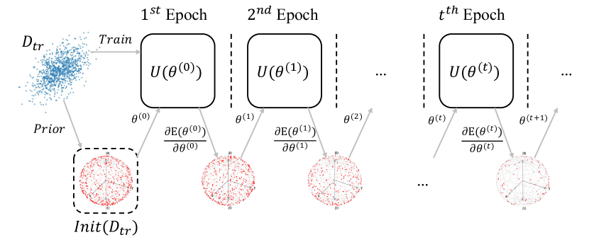
Figure 1: The overall process of our proposed strategy. Given a train data $D_{tr}$, we first initialize the model parameters with the prior knowledge of $D_{tr}$ as $\theta^{(0)}$ and feed both $D_{tr}$ and $\theta^{(0)}$ to the VQC $U(\cdot)$ for iterative training. In each iteration, let’s say in the $t^{th}$ iteration, we update $\theta^{(t)}$ with the gradient $\frac{\partial E(\theta^{(t)})}{\partial\theta^{(t)}}$ via a gradient-based approach and further diffuse Gaussian noise on model parameters $\theta^{(t+1)}$ for the next iteration.

Regularization with Prior Knowledge

Regularizing the model parameters via Bayesian inference is a popular regularization technique [31]. Specifically, the Bayesian approach can regularize the parameters by initializing the model weights using the approximated posterior distributions. This approach regards the model parameters $\theta$ as unknown variables and computes a posterior distribution ${\it P}\left(\theta\mid D\right)$ over $\theta$ given the data $D$ as a condition. According to the Bayes’ rule, the posterior can be approximated as follows:

$${\it P}\left(\theta\mid D\right)\propto{\it P}\left(D\mid\theta\right){\it P}\left(\theta\right),\\$$ (5)

where ${\it P}\left(D\mid\theta\right)$ denotes the maximum likelihood and ${\it P}\left(\theta\right)$ denotes the prior distribution of model parameters.

Employing posterior as the initial distribution of model parameters can provide a more robust initialization than only using maximum likelihood [14]. However, this approach has a significant drawback. For complex models, such as deep neural networks, it is not practical to compute the full probability distribution over model parameters due to high computational costs. To overcome this drawback, we simplify the process by considering the prior distribution of the given data $D$, such as the train data $D_{tr}$, as the initial distribution of model parameters. Our intuition is that utilizing such prior knowledge in initialization is equivalent to setting a constraint on the search space, thereby providing a robust initial optimization landscape against barren plateau issues. In Table I, we present the distinctions of three classic initial distributions between using original distributions (“Original”) and considering prior knowledge (“Ours”) as examples. We also visualize the initial distributions as an example to better demonstrate their distinctions among the three original distributions in Figure 2.

TABLE I: The distinctions of initialization between the original distributions and our distributions on three classic distributions. $D_{min}$ and $D_{max}$ denote the minimum and maximum values of the given data $D$, such as the train data $D_{tr}$ in the study. $\mu_{D}$, $\sigma_{D}$, $\alpha_{D}$, and $\beta_{D}$ denote the corresponding hyperparameters derived from the data $D$.

Distribution	Original	Ours
Uniform	$Uniform\left(0,1\right)$	$Uniform\left(D_{min},D_{max}\right)$
Normal	$Normal\left(0,1\right)$	$Normal\left(\mu_{D},\sigma_{D}\right)$
Beta	$Beta\left(0.5,0.5\right)$	$Beta\left(\alpha_{D},\beta_{D}\right)$

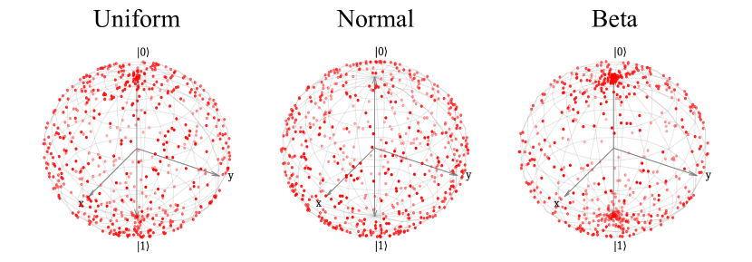
Figure 2: Example of three original distributions for initialization. The red points in this figure represent the initial values in model parameters.

Regularization with Gaussian Noise Diffusion

Besides the Bayesian approach, adding noise is another popular approach for regularization [32]. For example, BeInit [15] mitigates the degradation of gradient variance by adding Gaussian noise in the model parameters during training. However, adding too much noise will inevitably weaken the model’s performance [16]. Inspired by DDPM [17], which models better data distributions via an iterative Gaussian diffusion process, we iteratively diffuse the Gaussian noise on model weights during training. In the $t$-th iteration, we gradually diffuse the standard Gaussian noise $\epsilon\sim\mathcal{N}(0,I)$ to the diffused model parameters with a decreasing diffusion rate $\gamma$ as follows:

$$\left\{\begin{array}[]{lr}\overline{\theta^{(t)}}=\sqrt{\Gamma^{(t)}}\theta^{(t)},&\\ \overline{\epsilon}=\sqrt{(1-\Gamma^{(t)})}\epsilon,\end{array}\right.$$ (6)

where $\overline{\theta^{(t)}}$ and $\overline{\epsilon}$ denote the diffused parameters in the $t$-th iteration and diffused Gaussian noise; $\Gamma^{(t)}=\prod_{i=0}^{t}\gamma^{(i)}$ is the accumulated production of previous diffusion rates in the $t$-th iteration. The $\gamma$ linearly decreases with each iteration.

In each iteration, we apply the diffusion process on model parameters after back-propagation. The diffused parameters will be used in the next iteration. This diffusion process can be formulated as follows:

$$\theta^{(t+1)}=\overline{\theta^{(t)}}+\overline{\epsilon}.$$ (7)

As the number of iterations increases, the training will gradually converge, resulting in better model performance. Therefore, the model may require lower noise perturbations for regularization. Based on this intuition, we progressively diffuse the Gaussian noise on the model parameters as the optimization proceeds. We visualize the noise diffusion process in Figure 3 as an illustration example.

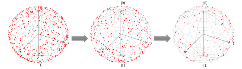
Figure 3: The process of diffusing Gaussian noise. The red points in this figure represent Gaussian noise added as regularization.

Input: Variational quantum circuits $U(\cdot)$, Train data $D_{tr}$, Learning rate, $\eta$, Train epochs $T$

1 $\theta^{(0)}\leftarrow Init\left(D_{tr}\right)$;

2 Compute $\Gamma=[\Gamma^{(0)},\Gamma^{(1)},...,\Gamma^{(T-1)}]$;

3 for $t=0\leftarrow T$ do

4       $\theta^{(t)}\leftarrow\theta^{(t)}-\eta\frac{\partial E(\theta^{(t)})}{\partial\theta^{(t)}}$;

5       $\overline{\theta^{(t)}}\leftarrow\sqrt{\Gamma^{(t)}}\theta^{(t)}$;

6       $\overline{\epsilon}\leftarrow\sqrt{(1-\Gamma^{(t)})}\epsilon$, where $\epsilon\sim\mathcal{N}(0,I)$;

7       $\theta^{(t+1)}\leftarrow\overline{\theta^{(t)}}+\overline{\epsilon}$;

8      

9 end for

Algorithm 1 Our training procedure.

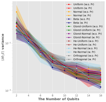
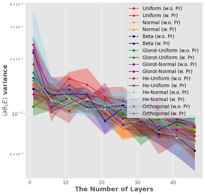
(a) Iris

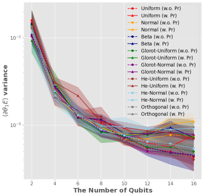
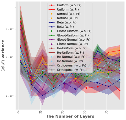
(b) Wine

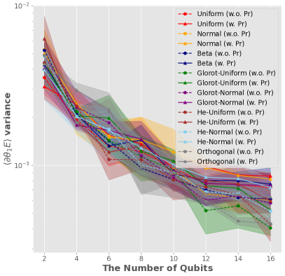
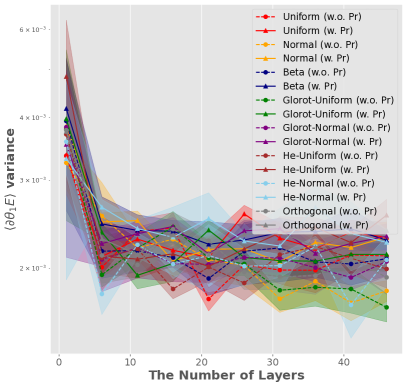
(c) Titanic

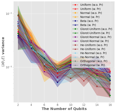
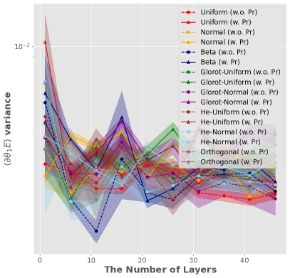
(d) MNIST

Figure 4: Investigation of the mechanism that leverages prior knowledge of the train data on eight popular initialization methods. “w. Pr” and “w.o. Pr” denote whether or not we apply prior knowledge.

The Training Procedure

As presented in Algo. 1, we first initialize the model parameters $\theta^{(0)}$ with the prior knowledge of the train data $D_{tr}$ (line 1), and then compute the hyperparameter, $\Gamma$, for each train step (line 2). After initialization, we train the variational quantum circuit $U(\cdot)$ with $T$ epochs (line 3-8). In the $t$-th iteration of the train loop, we update the model parameters $\theta^{(t)}$ via optimization approaches, such as gradient descent, with a learning rate $\eta$, where the gradient denotes $\frac{\partial E(\theta^{(t)})}{\partial\theta^{(t)}}$ (line 4). After updating the model parameters $\theta^{(t)}$, we apply diffusion to $\theta^{(t)}$ and Gaussian noise $\epsilon$ with $\Gamma^{(t)}$ using Equation 6 (line 5-6) and further update $\theta^{(t+1)}$ using Equation 7 for the next iteration (line 7).

Analysis of Time and Space Complexity

We propose two mechanisms for regularization in the training procedure. Regularizing the initial distribution with prior knowledge of the train data only implements once in line 1 and thus takes $\mathcal{O}(1)$. On the other hand, diffusing Gaussian noise to the model parameters $\theta^{(t)}$ takes constant time $\mathcal{O}(3)$ in each iteration (line 5-7). So, the total time complexity for $T$ train loops would be $\mathcal{O}(T+3)\approx\mathcal{O}(T)$. For the space complexity, initialization with prior knowledge does not take extra space, whereas diffusing Gaussian noise does require extra intermediate spaces for $\overline{\theta^{(t)}}$ and $\overline{\epsilon}$ in each iteration but these spaces are constant and will be released after each iteration. Thus, the total space complexity is still $\mathcal{O}(\theta)$. Overall, our proposed regularization methods will not theoretically increase the time and space complexity.

IV Experiments

In this section, We first present the settings and further verify the effectiveness of our method via ablation studies.

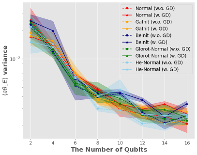
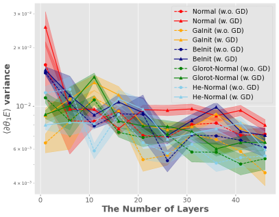
(a) Iris

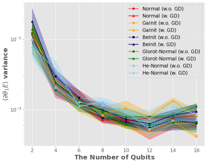
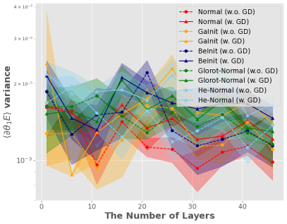
(b) Wine

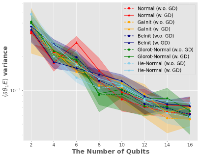
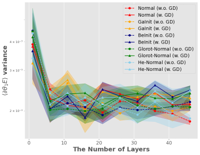
(c) Titanic

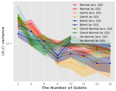
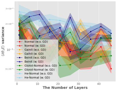
(d) MNIST

Figure 5: Investigation of the mechanism that regularizes model parameters by diffusing Gaussian noise along each iteration on five Gaussian-based methods. “w. GD” and “w.o. GD” denote whether or not we apply Gaussian noise diffusion.

Experimental Settings

In the experiment, we evaluate our proposed method across four public datasets. Iris is a classic machine-learning benchmark that measures various attributes of three-species iris flowers. Wine is a well-known dataset that includes 13 attributes of chemical composition in wines. Titanic contains historical data about passengers aboard the Titanic and is typically used to predict the survival. MNIST is a widely used small benchmark in computer vision. This benchmark consists of 28$\times$28 gray-scale images of handwritten digits from 0 to 9.

TABLE II: Statistics of datasets. $\left|D\right|$, $\left|F\right|$, and $\left|C\right|$ denote the original number of instances, features, and classes, respectively. “Splits” denotes the split instances for the train, validation, and test data.

Dataset	$\left|D\right|$	$\left|F\right|$	$\left|C\right|$	Splits
Iris	150	4	3	60:20:20
Wine	178	13	3	80:20:30
Titanic	891	11	2	320:80:179
MNIST	60,000	784	10	320:80:400

We refer to the settings of BeInit [15] and examine the VQCs in binary classification, i.e., we sub-sample instances from the first two classes in each dataset to build a new subset. After sub-sampling, we re-scale the feature size no larger than the number of qubits. The statistics of original datasets and the data splits for train, validation, and test sets are provided in Table II. Notably, the number of total sub-sampled instances is the sum of the split data. For example, in the Iris dataset, the number of sub-sampled instances is 100.

During training, we employ the Adam optimizer [8] to train VQCs with a learning rate of $1\times 10^{-2}$ and a batch size of 20. The Optimization converged within 50 training epochs. To assess the effectiveness of our proposed mechanisms, we ablatively apply the proposed mechanisms to baseline distributions, such as Gaussian initial distribution, and then observe the gap between two curves of gradient variance (whether or not our mechanism is applied to the baselines). We expect that after applying our mechanisms, the gap will become larger as the model size increases. Based on the above settings, we aim to ablatively investigate whether our proposed mechanisms can facilitate the trainability of VQCs in the following subsections.

Regularization with Prior Knowledge of The Train Data Can Help Alleviate Barren Plateaus

We conduct experiments to investigate whether prior knowledge can contribute to the initialization of the model parameters along different qubits or layers. In experiments, we include eight groups of initial distributions. For each group, we examine two scenarios, applying prior distributions to the initial distributions (“w. Pr”) or not (“w.o. Pr”). As presented in Figure 4, we repeat experiments five times and plot curves of the first-layer variance. We observe that in most cases, the variance in the first layer will gradually decrease as the number of qubits or layers increases. Besides, incorporating the prior distribution of the train data in initialization can mitigate barren plateau issues.

Regularization with Gaussian Noise Diffusion Can Help Avoid Being Trapped in Saddle Points

We conduct another ablation study to examine the effectiveness of our proposed regularization strategy. Specifically, we apply our proposed regularization strategy to both classic and state-of-the-art Gaussian-based methods and examine whether diffusing Gaussian noise on the model parameters along each training epoch as a regularization can help avoid being trapped in saddle points. We expect that this mechanism can increase volatility while alleviating the degradation of gradient variance during training. As presented in Figure 5, we repeat experiments five times and plot curves of the first-layer variance for each method. The results indicate that after applying Gaussian noise diffusion to the model parameters, in most Gaussian-based methods, the volatility of gradient variance increases so the optimization has a higher probability of avoiding being trapped in saddle points, whereas the gradient variance decreases much slower (i.e., the gap between two scenarios, “w.o. GD” and “w. GD”, becomes wider) as the number of qubits or layers increases, verifying the effectiveness of our proposed mechanism.

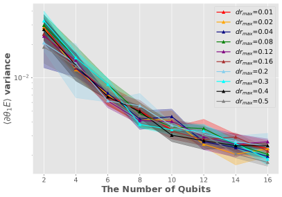
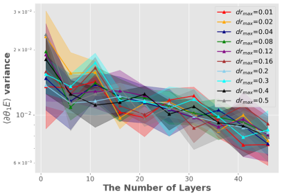
(a) Iris

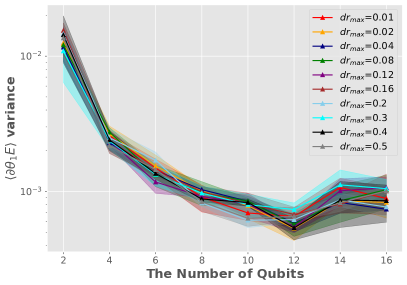
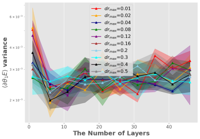
(b) Wine

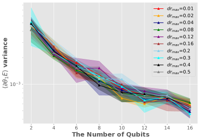
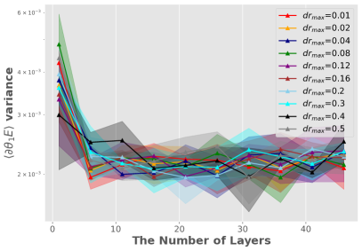
(c) Titanic

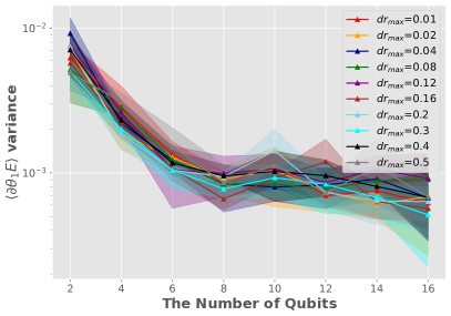
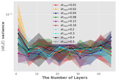
(d) MNIST

Figure 6: Analysis of the hyperparameter, $dr_{max}$, along different numbers of qubits or layers on four public datasets.

TABLE III: The optimal hyperparameter, max diffusion rate ($dr_{max}$) in each scenario. We report the results on Normal distribution as an example.

Dataset	Scenario	$dr_{max}$
Iris	Qubits	0.30
	Layers	0.02
Wine	Qubits	0.16
	Layers	0.01
Titanic	Qubits	0.20
	Layers	0.50
MNIST	Qubits	0.04
	Layers	0.02

Analysis of Hyperparameter

Besides verifying the effectiveness of our proposed methods, we fix the min diffusion rate ($dr_{min}$) as $1\times 10^{-4}$ and analyze the sensitivity of the key hyperparameter, max diffusion rate ($dr_{max}$), along different qubits or layers on the validation set. In this experiment, we simultaneously consider both mechanisms, i.e., applying prior knowledge of the train data in initialization and further diffusing Gaussian noise on model parameters along each training epoch. We repeat experiments five times on Normal distribution as an example and present curves of the first-layer variance for different $dr_{max}$ in Figure 6. We further compute the mean value of each curve (under different $dr_{max}$) and select the $dr_{max}$ in each scenario (either “qubits” or “layers” in each dataset) based on the maximum mean value. The optimal $dr_{max}$ for each scenario in this study is reported in Table III.

V Conclusion

In this study, we propose a regularization strategy integrated with two mechanisms to improve the trainability of variational quantum circuits (VQCs). First, we leverage prior knowledge of the train data to initialize the model parameters for mitigating barren plateau issues. Second, we regularize the model parameters by diffusing Gaussian noise during training to avoid being trapped in saddle points. In the experiment, we conduct ablation studies to verify the effectiveness of our proposed methods across four public datasets.

VI Limitations and Future Directions

In this study, we empirically verify the effectiveness of our proposed method. However, our method may fail to perform robustly due to the following limitations. First, we assume that the dataset follows a well-known distribution so we could regularize the initial distribution with prior knowledge of the train data. However, in real-life scenarios, data distributions may be more complex. This complexity may result in the failure to capture the true data distribution during initialization. Second, we assume that the distribution of the training data remains static during training. Based on this assumption, our method may be unable to adapt to the distribution shift since we predetermine the initial distribution of model parameters and the diffusion rate.

In the future, for the first limitation, we can employ non-parametric Bayesian approaches to capture the complex data distribution. To address the second limitation, we could handle the distribution-shift problem via detection-based methods (for detecting the shift) or adaptation-based methods (for adaptively updating the hyperparameters).

Appendix A Appendix

Hyper-parameters and Settings

In this study, we examine our proposed strategy on a baseline VQC, whose model architecture is described in Figure 7.

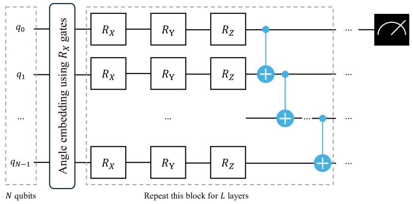
Figure 7: Model architecture of our baseline VQCs.

Hardware and Software

The experiment is conducted on a server with the following settings:

• Operating System: Ubuntu 22.04.3 LTS

• CPU: Intel Xeon w5-3433 @ 4.20 GHz

• GPU: NVIDIA RTX A6000 48GB

• Software: Python 3.11, PyTorch 2.1, Pennylane 0.31.1.

References

- [1] J. Preskill, “Quantum computing in the nisq era and beyond,” Quantum, vol. 2, p. 79, 2018.
- [2] B. Zhang, P. Xu, X. Chen, and Q. Zhuang, “Generative quantum machine learning via denoising diffusion probabilistic models,” Physical Review Letters, vol. 132, no. 10, p. 100602, 2024.
- [3] T.-Y. Chen, W.-Z. Zhang, R.-Z. Fang, C.-Z. Hang, and L. Zhou, “Multi-path photon-phonon converter in optomechanical system at single-quantum level,” Optics Express, vol. 25, no. 10, pp. 10 779–10 790, 2017.
- [4] T. Chen, J. Kim, M. Kuzyk, J. Whitlow, S. Phiri, B. Bondurant, L. Riesebos, K. R. Brown, and J. Kim, “Stable turnkey laser system for a yb/ba trapped-ion quantum computer,” IEEE Transactions on Quantum Engineering, vol. 3, pp. 1–8, 2022.
- [5] C. Zhan and H. Gupta, “Quantum sensor network algorithms for transmitter localization,” in 2023 IEEE International Conference on Quantum Computing and Engineering (QCE), vol. 1. IEEE, 2023, pp. 659–669.
- [6] C. Zhan, H. Gupta, and M. Hillery, “Optimizing initial state of detector sensors in quantum sensor networks,” ACM Transactions on Quantum Computing, 2023.
- [7] G. Li, Z. Song, and X. Wang, “Vsql: Variational shadow quantum learning for classification,” in Proceedings of the AAAI conference on artificial intelligence, 2021.
- [8] D. P. Kingma and J. Ba, “Adam: A method for stochastic optimization,” arXiv preprint arXiv:1412.6980, 2014.
- [9] J. R. McClean, S. Boixo, V. N. Smelyanskiy, R. Babbush, and H. Neven, “Barren plateaus in quantum neural network training landscapes,” Nature communications, vol. 9, no. 1, p. 4812, 2018.
- [10] R. Ge, F. Huang, C. Jin, and Y. Yuan, “Escaping from saddle points—online stochastic gradient for tensor decomposition,” in Conference on learning theory. PMLR, 2015, pp. 797–842.
- [11] C. Jin, R. Ge, P. Netrapalli, S. M. Kakade, and M. I. Jordan, “How to escape saddle points efficiently,” in International conference on machine learning. PMLR, 2017, pp. 1724–1732.
- [12] S. H. Sack, R. A. Medina, A. A. Michailidis, R. Kueng, and M. Serbyn, “Avoiding barren plateaus using classical shadows,” PRX Quantum, vol. 3, no. 2, p. 020365, 2022.
- [13] K. Zhang, L. Liu, M.-H. Hsieh, and D. Tao, “Escaping from the barren plateau via gaussian initializations in deep variational quantum circuits,” Advances in Neural Information Processing Systems, 2022.
- [14] S. J. Prince, Understanding Deep Learning. MIT press, 2023.
- [15] A. Kulshrestha and I. Safro, “Beinit: Avoiding barren plateaus in variational quantum algorithms,” in 2022 IEEE international conference on quantum computing and engineering (QCE). IEEE, 2022, pp. 197–203.
- [16] J. Zhuang and M. A. Hasan, “Robust node representation learning via graph variational diffusion networks,” arXiv preprint arXiv:2312.10903, 2023.
- [17] J. Ho, A. Jain, and P. Abbeel, “Denoising diffusion probabilistic models,” Advances in neural information processing systems, vol. 33, pp. 6840–6851, 2020.
- [18] L. Friedrich and J. Maziero, “Avoiding barren plateaus with classical deep neural networks,” Physical Review A, vol. 106, no. 4, p. 042433, 2022.
- [19] T. Haug and M. Kim, “Optimal training of variational quantum algorithms without barren plateaus,” arXiv preprint arXiv:2104.14543, 2021.
- [20] R. Selvarajan, M. Sajjan, T. S. Humble, and S. Kais, “Dimensionality reduction with variational encoders based on subsystem purification,” Mathematics, 2023.
- [21] S. Rappaport, G. Gyawali, T. Sereno, and M. J. Lawler, “Measurement-induced landscape transitions in hybrid variational quantum circuits,” arXiv preprint arXiv:2312.09135, 2023.
- [22] E. Grant, L. Wossnig, M. Ostaszewski, and M. Benedetti, “An initialization strategy for addressing barren plateaus in parametrized quantum circuits,” Quantum, 2019.
- [23] F. Sauvage, S. Sim, A. A. Kunitsa, W. A. Simon, M. Mauri, and A. Perdomo-Ortiz, “Flip: A flexible initializer for arbitrarily-sized parametrized quantum circuits,” arXiv preprint arXiv:2103.08572, 2021.
- [24] M. Ostaszewski, E. Grant, and M. Benedetti, “Structure optimization for parameterized quantum circuits,” Quantum, vol. 5, p. 391, 2021.
- [25] Y. Suzuki, H. Yano, R. Raymond, and N. Yamamoto, “Normalized gradient descent for variational quantum algorithms,” in 2021 IEEE International Conference on Quantum Computing and Engineering (QCE). IEEE, 2021, pp. 1–9.
- [26] V. Heyraud, Z. Li, K. Donatella, A. Le Boité, and C. Ciuti, “Efficient estimation of trainability for variational quantum circuits,” PRX Quantum, vol. 4, no. 4, p. 040335, 2023.
- [27] K. Bharti and T. Haug, “Quantum-assisted simulator,” Physical Review A, vol. 104, no. 4, p. 042418, 2021.
- [28] Y. Du, T. Huang, S. You, M.-H. Hsieh, and D. Tao, “Quantum circuit architecture search for variational quantum algorithms,” npj Quantum Information, vol. 8, no. 1, p. 62, 2022.
- [29] C. Tüysüz, G. Clemente, A. Crippa, T. Hartung, S. Kühn, and K. Jansen, “Classical splitting of parametrized quantum circuits,” Quantum Machine Intelligence, 2023.
- [30] M. Kashif and S. Al-Kuwari, “Resqnets: a residual approach for mitigating barren plateaus in quantum neural networks,” EPJ Quantum Technology, 2024.
- [31] J. Zhu, N. Chen, and E. P. Xing, “Bayesian inference with posterior regularization and applications to infinite latent svms,” The Journal of Machine Learning Research, vol. 15, no. 1, pp. 1799–1847, 2014.
- [32] H. Noh, T. You, J. Mun, and B. Han, “Regularizing deep neural networks by noise: Its interpretation and optimization,” Advances in neural information processing systems, vol. 30, 2017.