Configurable Learned Holography
Figure 1: Configurable Learned Holography. Our method presents a single-stage end-to-end learned approach for predicting 3D holograms and their corresponding laser powers from RGB-only 2D images. Our method supports various optical configurations using existing Spatial Light Modulators (SLMs) on the market without requiring retraining. Unique to our case in the literature, we eliminate the need for an additional stage for input depth estimation by simultaneously predicting depth and holograms in the same learned method. With the help of a knowledge-distillation technique, our final model can estimate hologram at interactive rates. We experimentally demonstrate 3D image reconstructions using two holographic display prototypes with different optical configurations to showcase our method in practice (Image Source: Creative Commons [Spragg(2009)]).

Abstract

In the pursuit of advancing holographic display technology, we face a unique yet persistent roadblock: the inflexibility of learned holography in adapting to various hardware configurations. This is due to the variances in the complex optical components and system settings in existing holographic displays. Although the emerging learned approaches have enabled rapid and high-quality hologram generation, any alteration in display hardware still requires a retraining of the model.

Our work introduces a configurable learned model that interactively computes 3D holograms from RGB-only 2D images for a variety of holographic displays. The model can be conditioned to predefined hardware parameters of existing holographic displays such as working wavelengths, pixel pitch, propagation distance, and peak brightness without having to retrain. In addition, our model accommodates various hologram types, including conventional single-color and emerging multi-color holograms that simultaneously use multiple color primaries in holographic displays. Notably, we enabled our hologram computations to rely on identifying the correlation between depth estimation and 3D hologram synthesis tasks within the learning domain for the first time in the literature. We employ knowledge distillation via a student-teacher learning strategy to streamline our model for interactive performance. Achieving up to a 2x speed improvement compared to state-of-the-art models while consistently generating high-quality 3D holograms with different hardware configurations.

Keywords: deep learning, neural networks, depth estimation, hard-parameter sharing, computer-generated holography

	Input	Speed	Hologram			SLM Refresh Rate	Stage	3D	Depth Accuracy	Learn	Max Z (mm)	VD (mm)	Con figur able
			Type	PD	DP
Our Method	RGB-only	Fast	M+S	8	No	60 Hz	Single	True	Moderate	Full	~10.0	~4.0	Yes
HoloBeam[Akşit and Itoh(2023)]	G-only	Fast	S	8	Yes	60 Hz	Single	True	Inaccurate	Full	~0.0	~6.0	No
Multi-DNN [Ishii et al.(2023)]	RGB-only	Slow	S	8	Yes	60 Hz	Three	True	Moderate	Full	~50.0	~2.0	No
NH [Peng et al.(2020)]	RGB-only	Fast	S	8	No	60 Hz	Two	False	Accurate	Full	~100.0	~12.5	No
NH3D [Choi et al.(2021a)]	RGB-D	Slow	S	8	No	60 Hz	Two	True	Accurate	Semi	~8.2	~4.4	No
TensorV2 [Shi et al.(2022)]	RGB-D	Fast	S	8	Yes	60 Hz	Two	True	Accurate	Full	~12.0	~6.0	No
DGE-CNN [Liu et al.(2023a)]	RGB-D	Slow	S	8	No	58 Hz	Two	True	Moderate	Semi	~10.0	~30.0	No
4K-DMDNet [Liu et al.(2023b)]	RGB-D	Slow	S	8	No	58 Hz	Two	False	Accurate	Full	~300.0	~40.0	No
Time-multiplexed [Choi et al.(2022a)]	RGB-D	Slow	S	4	No	480 Hz	Two	True	Accurate	Semi	~79.0	~12.0	No

Table 1: Comparison of hologram estimation methods. Our method can generate both single and multi-color holograms with accurate depth, RGB-only input and preferred optical configurations (Configurable). In Speed, Fast refers to $>10$ FPS, and Slow refers to $<10$ FPS. In Type, M refers to multi-color holograms and S refers to single-color holograms. In Learn, Full refers to the full learning-based method, and Semi refers to the semi learning-based method. The label PD refers to pixel depth. The label DP refers to double phase encoding [Hsueh and Sawchuk(1978)]. The label Z refers to propagation distance. The label VD refers to volume depth. SLM refers to Spatial Light Modulator.

1 Introduction

The technology offers immersive 3D visuals, paving the way for future advancements in display technologies. Despite its promising potential, holographic displays require complex computation [Blinder et al.(2019)], and more critically, hardware configurations such as optical component models and spatial placement. The recently emerging deep learning approaches have been advanced to address the computation bottleneck with real-time and high-quality hologram generation in both 2D and 3D [Shi et al.(2022)]. However, the models only accommodate a given preset optical configuration including working wavelengths, pixel pitch, propagation distance, and peak brightness. If applying the model to another end user’s display, they are not applicable and the whole system requires heavy retraining.

Our work focuses on generating Three-Dimensional (3D) holographic images in the variety of existing holographic displays. To achieve this goal, we introduce an end-to-end single-stage learned model capable of efficiently generating conventional single-color and emerging multi-color [Kavaklı et al.(2023b), Markley et al.(2023)] holograms at interactive rates. At its heart, our method identifies the correlation between depth estimation and hologram estimation tasks for the first time in the literature. The model adopts a strategy of hard-parameter sharing [Caruana(1993)] to yield high-quality hologram predictions straight from RGB-only input by predicting depth as a subtask. Our model can be conditioned for various optical configurations, including working wavelengths, pixel pitch, and peak brightness conditions, enabling a configurable approach compatible with different holographic display design choices. Furthermore, we use knowledge distillation through student-teacher learning strategy [Wang and Yoon(2021)] to unlock a learned model with lesser computational expense, supporting interactive rates. Our work introduces the following contributions:

• Configurable Hologram Estimation Model. We introduce a configurable hologram estimation model supporting a range of optical configurations from existing holographic displays and hologram types, including single and multi-color holograms.

• Single-stage Hologram Estimation from RGB-only inputs. Unlike previous methods with a dedicated depth estimation stage, our learned model leverages hard-parameter sharing to convert RGB-only images to holograms in a single stage, eliminating the need for an additional depth estimation step. This is the first time that the correlation between depth estimation and hologram estimation tasks has been identified in literature.

• Advancing Holograms towards Interactive Rates. We use knowledge distillation through a student-teacher learning strategy, we speed up our for interactive rate hologram estimation.

• Evaluations. We evaluate the image quality and speed of our model through an extensive study comparing against state-of-the-art hologram estimation methods and their potential future derivatives. We also verify our findings in two holographic display prototypes, demonstrating comparable image quality with the state-of-the-art in literature.

In pursuing our primary objective, we aspire for this research to serve as the first step in the development of self-configurable holographic displays, where future displays are envisioned to autonomously generate high-quality images, effectively adapting to varying optical configurations without compromising image quality.

2 Related Work

Our work deals with learned methods from inputs, and leverages multi-task learning using hard-parameter sharing. Here, we review relevant literature accordingly.

Learned Computer-Generated Holography.

Early works on conventional single-color hologram estimation utilize U-Net-based structures [Siddique et al.(2021)]. These methods require RGB-D inputs and are designed for specific optical configurations. A recent study by Shi et al. [Shi et al.(2022)] propose a stack of residual blocks without resolution reduction to speed up the estimation process for conventional single-color holograms. However, these methods [Shi et al.(2022)] still rely on RGB-D inputs. Liu  et al. [Liu et al.(2023a)] propose a two-stage solution for removing the dependency on depth information in the input (RGB-only). The first stage involves depth estimation, while the second stage optimizes conventional single-color holograms using RGB-only inputs. Akşit and Itoh [Akşit and Itoh(2023)] merge these two stages into a single stage while using RGB-only inputs. However, their estimated single-color holograms [Akşit and Itoh(2023)] provide inaccurate and limited depth in their reconstructed images. Ishii  et al. [Liu et al.(2023a)] propose a triple-stage solution where the first estimates depth, the second generates holograms using RGB-D input and the third optimizes the quality of the holograms. Our review suggests that the entirety of works in the literature are designed to work with a fixed preset optical configurations, typically requires RGB-D inputs and designed for single-color holograms. We provide a summary comparison of our method against the literature in Tbl. 1. Our work offers the first learned model to support various hologram typles, RGB-only inputs and a wide set of optical configurations. Currently, our method does not support heavily quantized holograms with 4-bit pixel depth [Choi et al.(2022b)], but only supports conventional single-color and emerging multi-color holograms with 8-bit pixel depth.

Multi-task Learning.

The work by Zhang and Yang [Zhang and Yang(2021)] introduces a comprehensive review of . Our work leverages [Caruana(1993)] to solve depth inaccuracies in previous works with RGB-only inputs [Akşit and Itoh(2023)], jointly learning input depths, holograms, and light source intensities using shared weights and biases. A common strategy in is to share layers among all tasks (hard-parameter sharing) while keeping output layers or several input layers (heads) task-specific [Ruder et al.(2019), Sarwar et al.(2019)]. Similarly, our work follows hard-parameter sharing while keeping only output heads task-specific. This approach is separate from soft-parameter sharing [Duong et al.(2015)], where each task has an independent , but other tasks constrain the weights of each . To our knowledge, our work is the first to identify that jointly learning subtasks of depth and hologram estimation can help estimate depth-accurate holograms when working with RGB-only inputs.

Knowledge Distillation.

[Hinton et al.(2015)] transfers knowledge from large models to introduce compact and lightweight models. is a powerful technique for reducing the computational costs of models in various tasks, including semantic segmentation [Liu et al.(2019)] and depth estimation [Pilzer et al.(2019)]. As mentioned in a survey by Gou  et al. [Gou et al.(2021)], methods follow teacher-student architecture. A teacher model can transfer knowledge to a student model either by regularizing the output responses (response-based) [Micaelli and Storkey(2019)] or layer responses (feature-based) [Chen et al.(2020)] between the two models. In the past, has also been applied in [Li and Bilen(2020)]. Following the findings from the work by Ignatov  et al. [Ignatov et al.(2021)], our work transfers knowledge from a teacher model based on to a student model through pixel-wise distillation (response-based). Our work is the first model to experiment with for accelerating the hologram estimation process in learned holography methods.

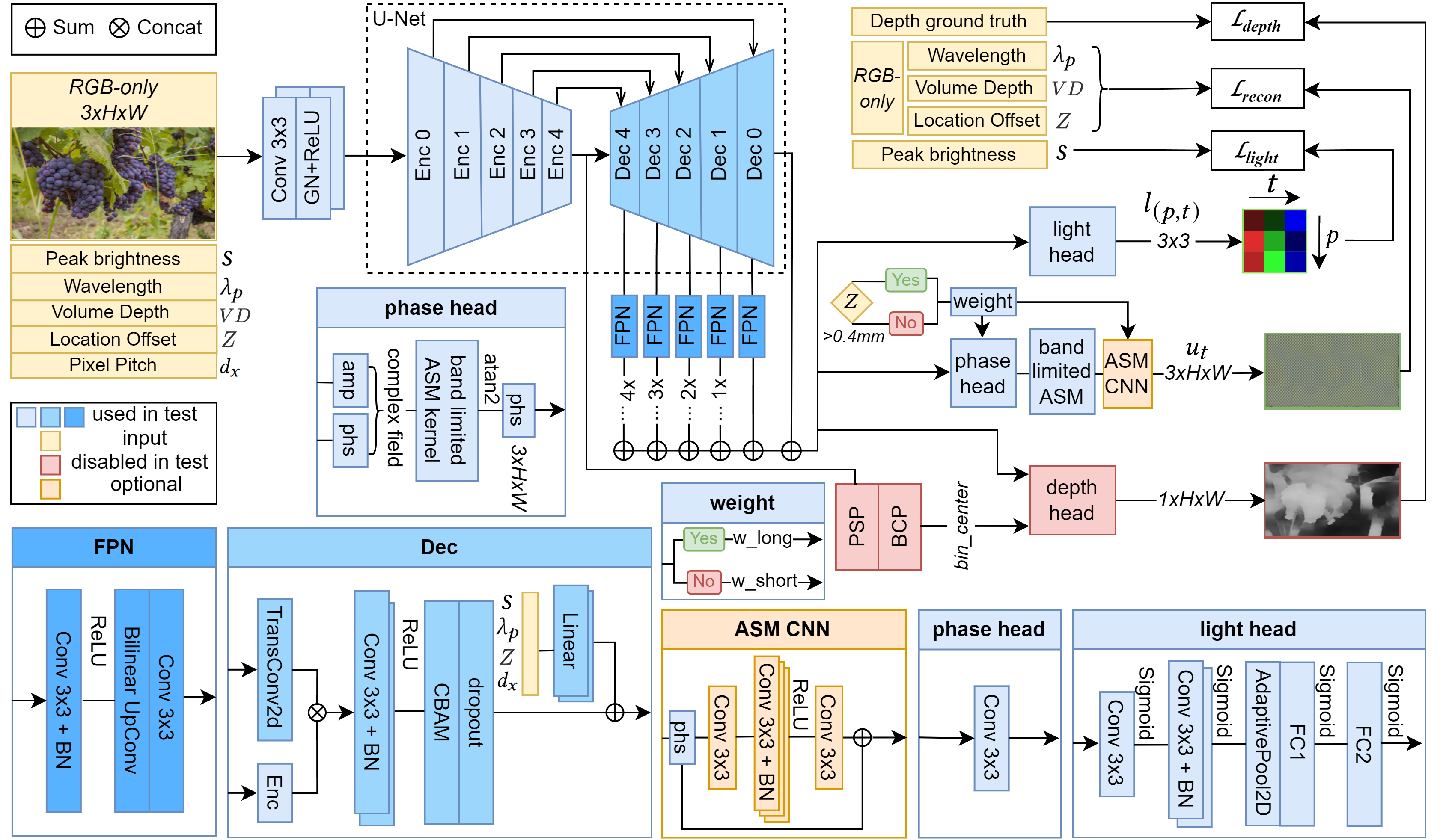
Figure 2: The overview of the teacher model. Based on the standard U-Net [Ronneberger et al.(2015)] structure, a  [Lin et al.(2016)] is connected to every stage of our U-Net’s decoder to leverage spatial information at varying scales from an input RGB-only input. Our method uses  [Woo et al.(2018)] to introduce both channel and spatial attention mechanisms, while each decoder is conditioned with optical characteristics, including peak brightness, wavelength, volume depth, location offset and pixel pitch. A Pyramid Spatial Pooling layer [He et al.(2014)] is integrated to enhance the model’s ability to aggregate spatial context for depth estimation. Our light head layer predicts required peak brightnesses. Our model uses two phase heads dedicated to long and short location offsets. Here, the $PSP$ represents the pyramid spatial pooling layer [He et al.(2014)], $BCP$ represents the  [Agarwal and Arora(2022)] (RGB-only input: Creative Commons [Bujar I Gashi 2012]).

3 Interactive 3D Holograms from 2D images

Our method estimates phase-only holograms that reconstruct scenes from RGB-only inputs while supporting single-color and multi-color hologram types. Here, we revisit the hologram generation formulation to introduce our method.

3.1 Synthesizing Single-color and Multi-color Holograms

Holographic displays play successive holograms rapidly to generate full-color images. In this process, the color primaries of holographic displays illuminate these holograms in accordance with their hologram type. The fuses the light from these illuminated holograms into full-color images. Suppose only a single-color primary illuminates a specific hologram, which is calculated for the particular wavelength of that single-color primary. In that case, this hologram type is single-color. In contrast, if multiple color primaries illuminate a specific hologram, and the hologram is calculated for all the wavelengths provided by these multiple color primaries, then this hologram is a multi-color hologram. Regardless of the hologram type, we could frame the hologram synthesis problem with the following minimization problem,

$$\hat{u}_{t},\hat{l}_{(p,t)}\leftarrow\operatorname*{argmin}_{u_{t},l_{(p,t)}}\underbrace{\sum_{p=1}^{P}\left\lVert\left(\sum_{t=1}^{T}\left\lvert l_{(p,t)}e^{i\frac{\lambda_{p}}{\lambda_{p_{\text{anchor}}}}u_{t}}*h_{p}\right\rvert^{2}\right)-sI_{p}\right\rVert_{2}^{2}}_{L_{\text{image}}},$$ (1)

where $P$ denotes the total number of color primaries (i.e. typically three in existing display technology), $p$ denotes the index of a color primary, $T$ denotes the total number of subframes reproducing a full-color image (i.e. typically three in holographic displays), $t$ denotes the index of a subframe, $l_{(t,p)}$ represents the peak brightness for the $p$-th primary at the $t$-th subframe, $\lambda_{p}$ denotes the wavelength of the active primary, $\lambda_{p_{\text{anchor}}}$ denotes the wavelength of the anchor primary, for which the nominal value of the SLM phase is calibrated against, $u_{t}$ represents the phase-only hologram (a subframe), $s$ represents the brightness scale, $h_{p}$ denotes the wavelength and location, $z$, dependent light transport kernel [Matsushima and Shimobaba(2009), Kavaklı et al.(2022), Choi et al.(2021b)], $I_{p}$ represents a parameter to scale the brightness of a target image intensity, and $L_{\text{image}}$ represents the visual difference between the intended target image for the given plane and reconstructed image by a hologram. Note that $l_{(p,t)}$ is by default an identity matrix in the single-color holograms, where only one color primary illuminates a subframe ($p=t$). Recent studies [Chao et al.(2023)] introduce improvements in brightness levels in single-color holograms. But the primary benefit of multi-color holograms concerning single-color is their support for a broader range of $s$. Thus, these multi-color holograms can support brighter images in holographic displays [Kavaklı et al.(2023b), Markley et al.(2023)] without requiring higher power light sources. We develop our learned model to support these two hologram types and their existing and potential benefits.

3.2 Estimating Single-color and Multi-color Holograms

Our final learned model is a student model that we refine from a teacher model using a knowledge distillation technique. Here, we introduce our teacher model and our fast student model.

3.2.1 Teacher Model

We provide a complete layout of our teacher model in Fig. 2. Our teacher model takes an RGB-only image, $I_{input}$, color primaries, $\lambda_{p}$, physical pixel pitch size, $d_{x}$, brightness scale, $s$, volume depth along propagation direction, $VD$, location offset, $Z$, as inputs in our training. Here, $Z$ refers to the propagation distance of the plane in the middle of $VD$. During our training, we vary some of these inputs for a given set of values so that our final trained model can condition the estimation process for preferred optical configurations at the test time. Specifically, our training draws the following variables from the below set in Eq. (2),

$$\begin{split}\lambda_{p}\subseteq\{(639,515,473)\}~{}nm,\\ s\subseteq\{1.0,1.4,1.8\},VD\subseteq\{4.0\}~{}mm,\\ Z\subseteq\{2,10\}~{}mm,d_{x}\subseteq\{3.74\}~{}\mu m.\end{split}$$ (2)

We generate permutations of our set in Eq. (2). These pairings are unique and don’t interchange in permutations. When training our teacher model, we train it for $I_{input}$, for a fixed setting chosen from permutations of our set in Eq. 2. Specifically, our configuration choice is as follows:

$$\begin{split}\lambda_{p}=(639,515,473)~{}nm,s=1.0\\ VD=4.0~{}mm,Z=10~{}mm,d_{x}=3.74~{}\mu m.\end{split}$$ (3)

As our teacher model is trained for the chosen fixed setting in Eq. (3), we further our training for $I_{input}$, using entire set of our permutations in one additional training session. In our teacher model as provided in Fig. 2, a U-Net structure [Ronneberger et al.(2015)] processes $I_{input}$. The encoder of our U-Net, $Enc$, is the EfficientNet 1B from the work by Tan and Le [Tan and Le(2019)]. EfficientNet [Tan and Le(2019)] is performant and memory-saving concerning other classical encoders (e.g. ResNet), which also guided our choice in design. In the decoder of our U-Net, $Dec$, the input from the previous layer goes into a transpose convolution layer, and the processed input is then concatenated with the input from the skip connection. The later stage in our decoder involves a [Woo et al.(2018)]. Note that is an attention-block that processes local information such as channel and spatial information, which we found necessary in our trials as it allowed us to estimate depth and reconstruct 3D images with our estimated holograms more accurately. The last stage of our decoder conditions our U-Net with $\lambda,s,d_{x}$. Specifically, we condition the variables using a that includes two consecutive fully connected layers. The conditioning enables our teacher model to estimate holograms for various optical configurations. We use features harvested from every level of our U-Net’s decoder and process it following the work by Lin  et al. [Lin et al.(2016)]. The features from various levels of our U-Net are processed with convolutional layers with batch normalization and a non-linear activation function of ReLU. Later, we upsample these features using bilinear filters. Finally, we process these upsampled features further using another set of convolutional layers with batch normalization and sum them all to form our latent code.

We provide the latent code of our teacher model to “heads” and dedicated to resolving three tasks, including predicting a phase-only hologram, peak brightness, and depth map of a given input image. We regularize the output of all tasks by using the following penalization term,

$$\mathcal{L}_{train}=\alpha_{0}\mathcal{L}_{recon}+\alpha_{1}\mathcal{L}_{light}+\alpha_{2}\mathcal{L}_{depth},$$ (4)

where $\alpha$s represents a set of hyperparameters ($\alpha_{0}=1,\alpha_{1}=1,\alpha_{2}=30$), $\mathcal{L}_{recon}$ represents multiplane image reconstruction loss as introduced by Kavaklı  et al. [Kavaklı et al.(2023a)], $\mathcal{L}_{light}$ represents light power constrain as introduced by Kavaklı  et al. [Kavaklı et al.(2023b)], and $\mathcal{L}_{depth}$ represents the depth estimation. In our implementation, we also compare the color performance of reconstructed images using regularizations from Andersson et al. [Andersson et al.(2020)]. This modification to $\mathcal{L}_{recon}$ is an addition to the original work by Kavakli et al. [Kavaklı et al.(2023a)] and helps improve color consistency in our reconstructions. Please refer to the supplementary materials for detailed information on specific aspects of our complete $\mathcal{L}_{train}$ implementation.

Phase-only hologram estimation task.

Our model has two branches for the phase-only hologram estimation task, each dedicated to a different range of $Z$. Specifically, if $Z$ is above $4~{}mm$, we load the long propagation weight $w\_long$ to phase head and ASM CNN denoted in Fig. 2, otherwise, we load the short propagation weight $w\_short$. The phase head consists of an identical convolutional layer. The output of the phase head provide pseudo amplitude and phase values, which are later converted into a complex-valued field. This complex-valued field is propagated using band-limited method using the same location offset $Z$ and wavelength $\lambda$ over all subframes. We later retrieve the phase from the complex-valued field as our phase-only hologram. As the last step, the phase will be fed into an additional ASM CNN, Note that as an extra step, when predicting long propagation distance hologram, the phase prediction will be fed into an additional ASM CNN, which consists of a convolution layer, followed by three consecutive convolution layers, batch normalization, and a nonlinear activation function ReLU. The end of the ASM CNN is a convolution layer. The output from this layer is combined with the previous phase from the complex field, culminating in the final phase output.

Light power estimation task.

The light head takes the latent code from the our teacher model as the input. In this head, the latent code will first be processed by a convolution layer and consecutive convolution layers with batch normalization and a sigmoid activation function. Next, the output from the previous layer will be fed into an adaptive pooling layer to aggregate the spatial information. Finally, the pooled output will be processed by two linear layers followed by a sigmoid activation function to make sure the shape of the prediction is $t$ x $p$ ($3\times 3$) and the data range is between 0 and 1.

Depth estimation task.

Our teacher model includes a dedicated depth head for this task. We feed the latent output of our U-Net and the bin center predictor’s output to our depth head as shown in Fig. 2. The bin center predictor cascades two modules: [He et al.(2014)] and [Agarwal and Arora(2022)]. . The bin center predictor estimates the distribution of depth values across different bins in the depth map, aiding precise depth prediction. We feed our U-Net’s last encoder layer output (Enc 4) into within the bin center predictor. In the depth head, the model’s latent code first passes through a depthwise convolution layer and a Softmax activation function. Then, we multiply the softmax layer’s output by the bin center prediction to generate the final depth prediction. We apply regularization to the depth estimations from the depth head using a loss function, $\mathcal{L}_{depth}$, the sum of three sub-loss functions without any weights: $\mathcal{L}_{silog}$, $\mathcal{L}_{gm}$, and $\mathcal{L}_{tv}$. The scale-invariant loss, $\mathcal{L}_{silog}$, is introduced by eigen  et al. in [Eigen et al.(2014)]. The gradient matching loss, $\mathcal{L}_{gm}$, compares the edges of estimated depths with ground truth depth maps. The total variant loss, $\mathcal{L}_{tv}$, smoothes the edges of objects in the depth map. For more information on implementing $\mathcal{L}_{depth}=\mathcal{L}_{silog}+\mathcal{L}_{gm}+\mathcal{L}_{tv}$, refer to our supplementary materials.

3.2.2 Student Model.

Our teacher model can be enhanced by transforming it into a simpler student model through the knowledge distillation technique [Wang and Yoon(2021)], which allows for more rapid estimation of 3D phase-only holograms. Firstly, we present a comprehensive layout of our student model in Fig. 3. Similar to the teacher model, the student model also takes $I_{input}$, $\lambda_{p}$, $d_{x}$, $s$, $VD$, and $Z$ as inputs. Furthermore, our student model employs the U-Net structure to process $I_{input}$, but with a different encoder - MobileNetV3 [Howard et al.(2019)] . MobileNetV3 serves as a more compact alternative to the teacher model’s encoder, often used for lightweight models due to its efficiency. In our student decoders, similar to the teacher model, the input from the previous layer also goes into a transpose convolution layer, and the processed input is then concatenated with the input from the skip connection. Concatenated information is processed by a consecutive depthwise separable convolution layer with batch normalization and a nonlinear ReLU activation function. The last stage of our student decoder conditions our U-Net with $\lambda,s,d_{x}$ as well. The structure of the linear condition layers remains the same as the teacher model. The structures of the prediction heads in the student model are also the same as the teacher model.

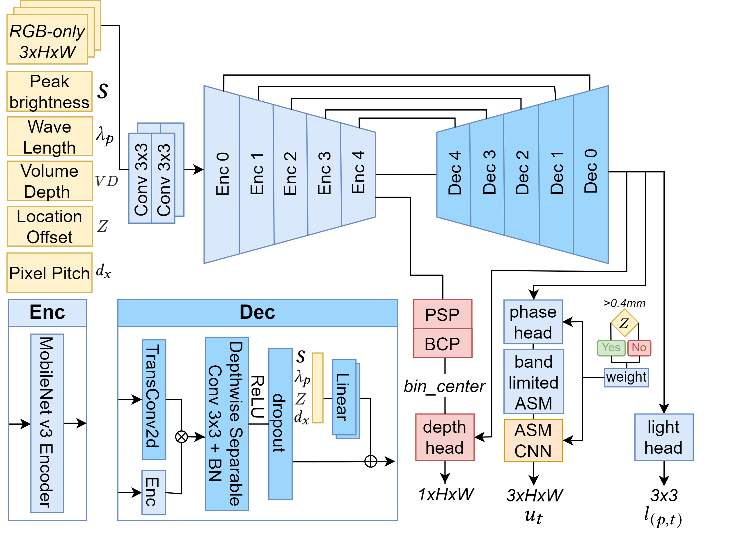
Figure 3: The overview of the student model.

In training of our student model, the logit based [Hinton et al.(2015)] is applied to balance the model performance and the inference speed. The original knowledge distillation loss $\mathcal{L}_{KD}$, is defined as:

$$\mathcal{L}_{KD}=T^{2}\cdot D_{KL}(S(y_{student}/T),S(y_{teacher}/T)).$$ (5)

Here, $D_{KL}$ represents the Kullback-Leibler divergence [Kullback(1951)], $y_{student}$ and $y_{teacher}$ are the phase and depth predictions of the student and teacher models, and $S$ denotes the softmax function. The temperature parameter $T$ controls the softness of probabilities. The scalar factor $T^{2}$ is used to scale the loss back to the correct magnitude. However, $\mathcal{L}_{KD}$ only captures the overall data distribution, the information of the edge and the texture of the depth map will be missing. To have a robust and accurate depth distillation, we combined the $\mathcal{L}_{KD_{depth}}$ with the depth estimation loss $\mathcal{L}_{depth}$. The target of the $\mathcal{L}_{depth}$ will be depth map prediction from the teacher model instead of the ground truth depth. Additionally, since the student model’s capacity is much smaller than the teacher model, we found that during training, the student model finds it hard to maintain a smooth phase prediction. To resolve this issue, we involved Charboninner loss [Barron(2017)] as our pixel-wise distillation loss of phase prediction between the student and teacher model. The updated distillation loss $\mathcal{L}_{distill}$ will be defined as $\mathcal{L}_{distill}=\mathcal{L}_{KD_{phase}}+\mathcal{L}_{charboninner}+\mathcal{L}_{KD_{depth}}+\mathcal{L}_{depth}$. The final loss that combines the original training loss and the knowledge distillation loss is defined as:

$$\mathcal{L}=\mathcal{L}_{distill}+\mathcal{L}_{train}.$$ (6)

3.3 Implementation

We used the dataset SA-1B, omitting the masks, in our training sessions for teacher and student model. Furtermore, we employed the MiDaS [Lasinger et al.(2019)] for generating ground truth depth for these images. Due to limitations in computational resources and time, our usage was confined to a subset of the dataset, specifically 30,000 images, which represents approximately $0.3\%$ of the entire dataset. We implemented our method using Pytorch [Paszke et al.(2019)]. We use Adam [Kingma and Ba(2015)] optimizer ($\beta_{1}=0.9,\beta_{2}=0.99$), with batch size 16 and CosineAnnealingLR [Loshchilov and Hutter(2016)] as the scheduler. The teacher model and student model were trained individually under the same training setting. Specifically, the teacher model was trained with 30K images at the resolution of 768 x 768, while the student model utilized a smaller set of 20,000 images at the resolution of 1024 x 1024. Both models are trained for 20 epochs with an initial of 0.001, which was progressively reduced following a cosine decay function. All experiments were conducted on eight NVIDIA RTX 3090 24G GPUs, and no data augmentation techniques were employed during the training process. The total time of training teacher model and distilling student model roughly takes 4.5 days. Training our teacher model for a wide variety of optical configurations could easily exhaust computational resources. To prove the validity of our approach, in parallel we also derive a version of our teacher model that works with RGB-D inputs where depth prediction task is not involved. we trained the model with another variable set containing various volume depths, wavelengths, and pixel pitches. The result is available in supplementary materials.

Method	Input	Optical Configuration	PSNR↑ (dB)	SSIM↑	LPIPS↓	FLIP↓	Para meters	Speed
Our Method (teacher)	RGB-only	$d_{x}$: 3.74 µm, Z: 2 mm, VD: 4 mm, x1.0	30.45$\pm$2.43	0.95$\pm$0.03	0.35	0.09	10.74 M	769 ms
		$d_{x}$: 3.74 µm, Z: 2 mm, VD: 4 mm, x1.4	24.66$\pm$1.80	0.90$\pm$0.04	0.47	0.26
		$d_{x}$: 3.74 µm, Z: 2 mm, VD: 4 mm, x1.8	29.19$\pm$2.37	0.91$\pm$0.04	0.38	0.12
		$d_{x}$: 3.74 µm, Z: 10 mm, VD: 4 mm, x1.0	23.72$\pm$1.37	0.90$\pm$0.04	0.60	0.27
		$d_{x}$: 3.74 µm, Z: 10 mm, VD: 4 mm, x1.4	21.75$\pm$1.34	0.83$\pm$0.04	0.73	0.34
		$d_{x}$: 3.74 µm, Z: 10 mm, VD: 4 mm, x1.8	21.39$\pm$1.28	0.84$\pm$0.03	0.71	0.36
Our Method (student)	RGB-only	$d_{x}$: 3.74 µm, Z: 2 mm, VD: 4 mm, x1.0	29.89$\pm$2.80	0.96$\pm$0.03	0.35	0.08	2.18 M	42 ms
		$d_{x}$: 3.74 µm, Z: 2 mm, VD: 4 mm, x1.4	30.14$\pm$2.71	0.96$\pm$0.04	0.36	0.09
		$d_{x}$: 3.74 µm, Z: 2 mm, VD: 4 mm, x1.8	29.01$\pm$2.64	0.94$\pm$0.05	0.38	0.11
		$d_{x}$: 3.74 µm, Z: 10 mm, VD: 4 mm, x1.0	25.87$\pm$1.60	0.87$\pm$0.04	0.46	0.17
		$d_{x}$: 3.74 µm, Z: 10 mm, VD: 4 mm, x1.4	25.49$\pm$1.62	0.88$\pm$0.04	0.44	0.17
		$d_{x}$: 3.74 µm, Z: 10 mm, VD: 4 mm, x1.8	24.34$\pm$1.85	0.86$\pm$0.04	0.47	0.18
HoloBeam	RGB-only*	$d_{x}$: 3.74 µm, Z: 2 mm, VD: 4 mm, x1.0	29.12$\pm$2.70	0.93$\pm$0.04	0.37	0.10	1.94 M	27 ms
		$d_{x}$: 3.74 µm, Z: 0 mm, VD: 6 mm, x1.0	28.75$\pm$2.84	0.93$\pm$0.04	0.38	0.11
TensorHolo V2	RGB-D	$d_{x}$: 8.0 µm, Z: 0 mm, VD: 6 mm, x1.0	29.27$\pm$3.39	0.97$\pm$0.03	0.29	0.09	0.04 M	75 ms
		$d_{x}$: 8.0 µm, Z: 12 mm, VD: 6 mm, x1.0	22.78$\pm$1.45	0.96$\pm$0.03	0.31	0.09
modified 3D NH**	RGB-D	$d_{x}$: 3.74 µm, Z: 2 mm, VD: 4 mm, x1.0	29.01$\pm$2.45	0.94$\pm$0.03	0.40	0.11	3.87 M	49 ms
		$d_{x}$: 3.74 µm, Z: 100 mm, VD: 12.5 mm, x1.0***	28.92$\pm$3.25	0.87$\pm$0.04	0.47	0.13
		$d_{x}$: 8.0 µm, Z: 2 mm, VD: 4 mm, x1.0	31.15$\pm$2.08	0.95$\pm$0.02	0.37	0.10
		$d_{x}$: 8.0 µm, Z: 100 mm, VD: 12.5 mm, x1.0***	30.79$\pm$2.98	0.90$\pm$0.03	0.43	0.10

Table 2: Evaluation of various models at different holography settings. The test resolution is at 1920 x 1080. Parameters refers to the size of the model. Speed refers to the inference time of the model. Note that Our Method (RGB teacher), Our Method (RGB student), HoloBeam, TensorHolo V2 and modified 3D NH used 768 x 768, 1024 x 1024, 1024 x 1024, 384 x 384 and 1024 x 1024 resolution to train, respectively. ^*We improve the model from G-only to RGB-only input. ^**In our experiment, training modified 3D NH with 1024 x 1024 resolution for long propagation distance will cause image quality to drop severely. Hence, we used 1920 x 1080 resolution to train the long propagation version of modified 3D NH. ^***Since NH only supports 2D holograms, we modified NH‘s HoloNet [Peng et al.(2020)] to enable 3D holograms generation. For more details of modified 3D NH, please consult the supplementary materials.

4 Evaluation and Discussion

Quantitative Analysis

In  Tbl. 2, we calculated the mean and standard deviation for PSNR, SSIM, LPIPS [Zhang et al.(2018)], and FLIP [Andersson et al.(2020)]. The metrics for this assessment were obtained using 100 images from the DIV2K dataset [Agustsson and Timofte(2017)]. First, concerning the other models in Tbl. 2, the student model can generate 3D holograms with different optical configurations without compromising the image quality. The observation is evidenced by the fact that the overall PNSR/SSIM only marginally changed $7.9\%$ and $4.4\%$. For LPIPS, though TensorHolo V2 has the highest value, overall the student model is as good as the modified 3D NH and HoloBeam. For FLIP, student model achieves the highest value. Besides the numerical analysis, we also employ pair-wise ANOVA test as the statistical analysis to evaluate the significance of these metrics, which is readily available in supplementary. Second, in line with existing iterative methods [Kavaklı et al.(2023b)], increasing the peak brightness or propagation distance tend to lower image quality in the student model. For example, 1.8 brightness induces the decrease of $3.0\%$, $2.1\%$, $8.6\%$ and $37.5\%$ in PSNR, SSIM, LPIPS and FLIP, respectively. This trend is consistent across different configurations and methods. Lastly, due to the absence of feature aggregation components, the student model outperforms the teacher model by $10.4\%$, $2.7\%$, $20.1\%$ and $36.8\%$ in PSNR, SSIM, LPIPS and FLIP, respectively, which evidences the effectivness of the student model design. Although these components are essential in improving depth accuracy, the pooling and upsample operations adversely affect phase prediction.

Qualitative Analysis

We evaluate our method, student model, using simulation results. In addition, we provide experimental results from two actual holographic display prototypes in our supplementary. Fig. 4 shows the reconstruction results of student model at short propagation distance, where reconstructions provides fine details across various peak brightness levels. Our method demonstrated a high degree of fidelity in the reconstruction of fine details and texture preservation in different peak brightnesses. The model managed to retain the structural integrity and color accuracy of the original images. Fig. 5 shows the reconstruction results of student model at long propagation distance. Compared with short propagation distance, the long propagation distance results reveal a noticeable deviation in color from the ground truth. This deviation is due to the challenges of long propagation distance tasks, which require a larger training resolution for the model to fit the high-resolution data and the long propagation distance. The student model is distilled using data at a resolution of $1024\times 1024$, which is smaller than the test resolution 1920 x 1080. Due to limitation of computational resources and time, we were unable to utilize larger images for RGB-only model training. To validate our point, we used full HD data to train our RGB-D condition model for long propagation distance and compared with modified 3D NH and TensorHolo V2, the result is readily available in our supplementary materials.

Discussion

Our research facilitates the generation of configurable 3D holograms at interactive rate. However, the current model can not adapt beyond pre-existing conditions, it still requires retraining for new optical configurations. Our ultimate goal is to make the model continuous configurable, meaning the model can adapt to novel configurations outside of the variable set. Inspired by Towaki  et al. [Takikawa et al.(2023)], a potential approach might involve training separate models for each single optical configuration. When a new configuration is required, a selective combination of weights from these models could be utilized to interpolate and adjust the model’s output to meet the new conditions. Besides the inability of continuous configurable, our solution has the following limitations: Extended Training Time. Although linear condition layers can help the model to understand the difference between different holographic settings, the number of permutations of the condition settings increases exponentially when the size of the variables set increases. This will lead to longer training time. The original variable set of our paper also contains different wavelengths and pixel pitches, however having such a large variable set takes weeks to train. The lack of scalability of . The performance of significantly decreases with the escalation of test image resolutions. This is due to the model’s training, which is limited to the current or lower resolution scales, impeding its ability to generalize patterns at higher resolutions. Consequently, this limitation affects the accuracy of hologram defocus regions, as depth estimation result directly influences the focus regions. Testing images at large resolution may thus erroneously defocus some areas that are meant to be in focus at given depth plane.

An emerging next-generation display method, holographic display technology has shown remarkable improvements, particularly in applications akin to glasses [Jang et al.(2022)]. These advancements require corresponding innovations in computational methods to fully realize their potential in enhancing user experiences and facilitating their integration into everyday use.

In conclusion, we have presented the first approach to create multi-color 3D holograms from RGB-only inputs for various display configurations. Most importantly, our work unearthed the connection between depth estimation and 3D hologram generation tasks, a first in this field.

Figure 4: The short propagation distance reconstructions comparison of student model when peak brightness are 1.0, 1.4, and 1.8. The volume depth of the results is 4mm and the location offset is 2mm (Image Source: Creative Commons [Eric Hunt 2003]).

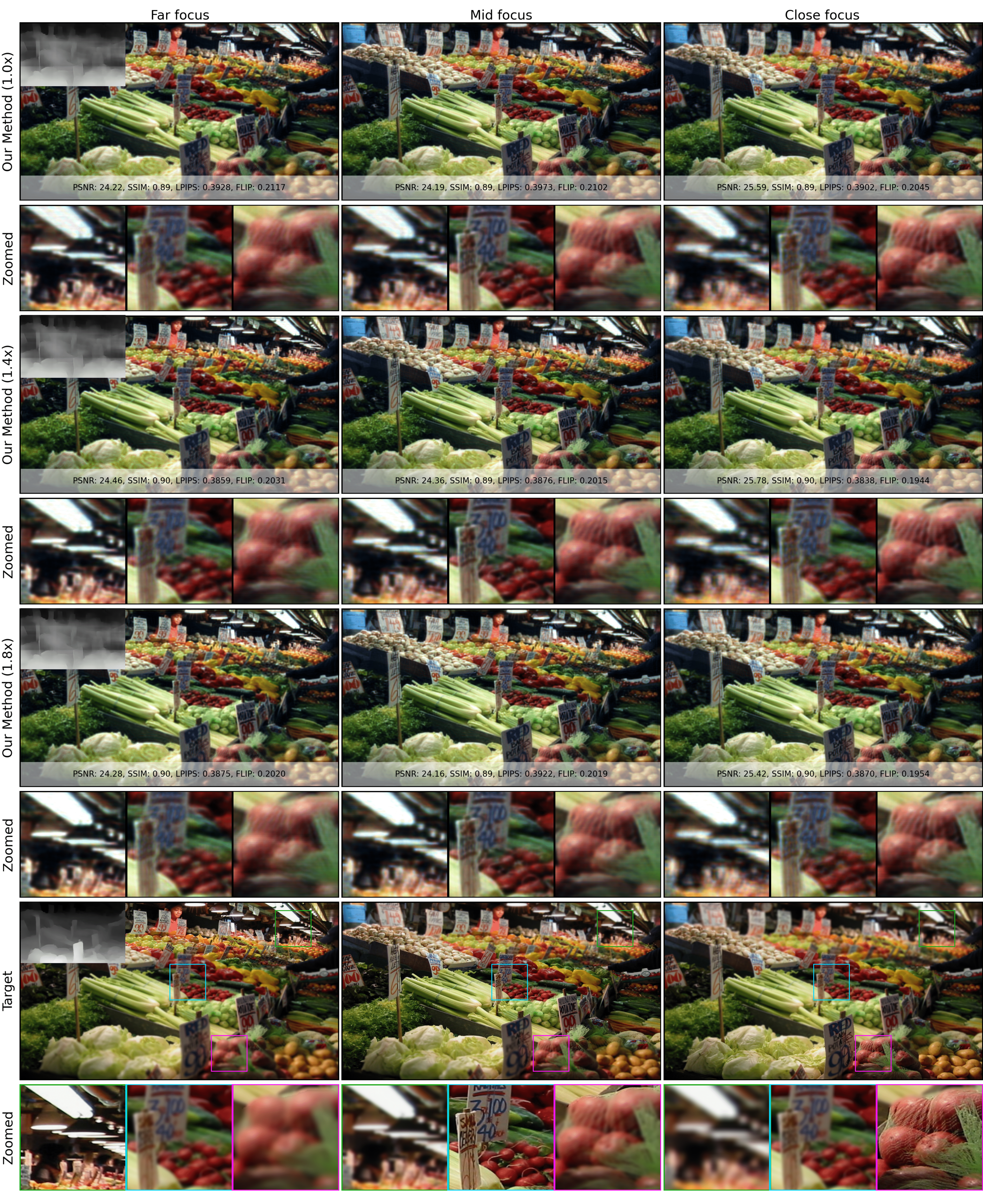
Figure 5: The long propagation distance reconstructions comparison of student model when peak brightness are 1.0, 1.4, and 1.8. The volume depth of the results is 4mm and the location offset is 10mm (Image Source: Creative Commons [Eric Hunt 2003]).

References

- [1]
- [Agarwal and Arora(2022)] Ashutosh Agarwal and Chetan Arora. 2022. Attention Attention Everywhere: Monocular Depth Prediction with Skip Attention. arXiv:2210.09071 [cs.CV]
- [Agustsson and Timofte(2017)] Eirikur Agustsson and Radu Timofte. 2017. NTIRE 2017 Challenge on Single Image Super-Resolution: Dataset and Study. In The IEEE Conference on Computer Vision and Pattern Recognition (CVPR) Workshops.
- [Akşit and Itoh(2023)] Kaan Akşit and Yuta Itoh. 2023. HoloBeam: Paper-Thin Near-Eye Displays. In 2023 IEEE Conference Virtual Reality and 3D User Interfaces (VR). IEEE, 581–591.
- [Andersson et al.(2020)] Pontus Andersson, Jim Nilsson, Tomas Akenine Moller, Magnus Oskarsson, Kalle AAstrom, and Mark D. Fairchild. 2020. FLIP: A Difference Evaluator for Alternating Images. Proceedings of the ACM on Computer Graphics and Interactive Techniques 3, 2 (2020), 15:1–15:23. https://doi.org/10.1145/3406183
- [Barron(2017)] Jonathan T. Barron. 2017. A More General Robust Loss Function. CoRR abs/1701.03077 (2017). arXiv:1701.03077 http://arxiv.org/abs/1701.03077
- [Blinder et al.(2019)] David Blinder, Ayyoub Ahar, Stijn Bettens, Tobias Birnbaum, Athanasia Symeonidou, Heidi Ottevaere, Colas Schretter, and Peter Schelkens. 2019. Signal processing challenges for digital holographic video display systems. Signal Processing: Image Communication 70 (2019), 114–130.
- [Caruana(1993)] R Caruana. 1993. Multitask learning: A knowledge-based source of inductive bias1. In Proceedings of the Tenth International Conference on Machine Learning. Citeseer, 41–48.
- [Chao et al.(2023)] Brian Chao, Manu Gopakumar, Suyeon Choi, and Gordon Wetzstein. 2023. High-brightness holographic projection. Optics Letters 48, 15 (2023), 4041–4044.
- [Chen et al.(2020)] Hanting Chen, Yunhe Wang, Chang Xu, Chao Xu, and Dacheng Tao. 2020. Learning student networks via feature embedding. IEEE Transactions on Neural Networks and Learning Systems 32, 1 (2020), 25–35.
- [Choi et al.(2022a)] Suyeon Choi, Manu Gopakumar, Yifan Peng, Jonghyun Kim, Matthew O’Toole, and Gordon Wetzstein. 2022a. Time-multiplexed Neural Holography: A Flexible Framework for Holographic Near-eye Displays with Fast Heavily-quantized Spatial Light Modulators. In SIGGRAPH ’22: Special Interest Group on Computer Graphics and Interactive Techniques Conference, Vancouver, BC, Canada, August 7 - 11, 2022, Munkhtsetseg Nandigjav, Niloy J. Mitra, and Aaron Hertzmann (Eds.). ACM, 32:1–32:9. https://doi.org/10.1145/3528233.3530734
- [Choi et al.(2022b)] Suyeon Choi, Manu Gopakumar, Yifan Peng, Jonghyun Kim, Matthew O’Toole, and Gordon Wetzstein. 2022b. Time-multiplexed Neural Holography: A Flexible Framework for Holographic Near-eye Displays with Fast Heavily-quantized Spatial Light Modulators. In SIGGRAPH ’22: Special Interest Group on Computer Graphics and Interactive Techniques Conference, Vancouver, BC, Canada, August 7 - 11, 2022, Munkhtsetseg Nandigjav, Niloy J. Mitra, and Aaron Hertzmann (Eds.). ACM, 32:1–32:9. https://doi.org/10.1145/3528233.3530734
- [Choi et al.(2021a)] Suyeon Choi, Manu Gopakumar, Yifan Peng, Jonghyun Kim, and Gordon Wetzstein. 2021a. Neural 3D holography: learning accurate wave propagation models for 3D holographic virtual and augmented reality displays. ACM Trans. Graph. 40, 6 (2021), 240:1–240:12. https://doi.org/10.1145/3478513.3480542
- [Choi et al.(2021b)] Suyeon Choi, Manu Gopakumar, Yifan Peng, Jonghyun Kim, and Gordon Wetzstein. 2021b. Neural 3D holography: learning accurate wave propagation models for 3D holographic virtual and augmented reality displays. ACM Transactions on Graphics (TOG) 40, 6 (2021), 1–12.
- [Duong et al.(2015)] Long Duong, Trevor Cohn, Steven Bird, and Paul Cook. 2015. Low resource dependency parsing: Cross-lingual parameter sharing in a neural network parser. In Proceedings of the 53rd annual meeting of the Association for Computational Linguistics and the 7th international joint conference on natural language processing (volume 2: short papers). 845–850.
- [Eigen et al.(2014)] David Eigen, Christian Puhrsch, and Rob Fergus. 2014. Depth Map Prediction from a Single Image using a Multi-Scale Deep Network. CoRR abs/1406.2283 (2014). arXiv:1406.2283 http://arxiv.org/abs/1406.2283
- [Gou et al.(2021)] Jianping Gou, Baosheng Yu, Stephen J Maybank, and Dacheng Tao. 2021. Knowledge distillation: A survey. International Journal of Computer Vision 129 (2021), 1789–1819.
- [He et al.(2014)] Kaiming He, Xiangyu Zhang, Shaoqing Ren, and Jian Sun. 2014. Spatial Pyramid Pooling in Deep Convolutional Networks for Visual Recognition. CoRR abs/1406.4729 (2014). arXiv:1406.4729 http://arxiv.org/abs/1406.4729
- [Hinton et al.(2015)] Geoffrey Hinton, Oriol Vinyals, and Jeff Dean. 2015. Distilling the knowledge in a neural network. arXiv preprint arXiv:1503.02531 (2015).
- [Howard et al.(2019)] Andrew Howard, Mark Sandler, Grace Chu, Liang-Chieh Chen, Bo Chen, Mingxing Tan, Weijun Wang, Yukun Zhu, Ruoming Pang, Vijay Vasudevan, Quoc V. Le, and Hartwig Adam. 2019. Searching for MobileNetV3. CoRR abs/1905.02244 (2019). arXiv:1905.02244 http://arxiv.org/abs/1905.02244
- [Hsueh and Sawchuk(1978)] Chung-Kai Hsueh and Alexander A Sawchuk. 1978. Computer-generated double-phase holograms. Applied optics 17, 24 (1978), 3874–3883.
- [Ignatov et al.(2021)] Andrey Ignatov, Grigory Malivenko, David Plowman, Samarth Shukla, and Radu Timofte. 2021. Fast and accurate single-image depth estimation on mobile devices, mobile ai 2021 challenge: Report. In Proceedings of the IEEE/CVF Conference on Computer Vision and Pattern Recognition. 2545–2557.
- [Ishii et al.(2023)] Yoshiyuki Ishii, Fan Wang, Harutaka Shiomi, Takashi Kakue, Tomoyoshi Ito, and Tomoyoshi Shimobaba. 2023. Multi-depth hologram generation from two-dimensional images by deep learning. Optics and Lasers in Engineering 170 (2023), 107758. https://doi.org/10.1016/j.optlaseng.2023.107758
- [Jang et al.(2022)] Changwon Jang, Kiseung Bang, Minseok Chae, Byoungho Lee, and Douglas Lanman. 2022. Waveguide Holography: Towards True 3D Holographic Glasses. CoRR abs/2211.02784 (2022). https://doi.org/10.48550/ARXIV.2211.02784 arXiv:2211.02784
- [Kavaklı et al.(2023a)] Koray Kavaklı, Yuta Itoh, Hakan Urey, and Kaan Akşit. 2023a. Realistic defocus blur for multiplane computer-generated holography. In 2023 IEEE Conference Virtual Reality and 3D User Interfaces (VR). IEEE, 418–426.
- [Kavaklı et al.(2023b)] Koray Kavaklı, Liang Shi, Hakan Urey, Wojciech Matusik, and Kaan Akşit. 2023b. Multi-color Holograms improve Brightness in Holographic Displays. In ACM SIGGRAPH ASIA 2023 Conference Proceedings. –. https://doi.org/10.1145/3610548.3618135
- [Kavaklı et al.(2022)] Koray Kavaklı, Hakan Urey, and Kaan Akşit. 2022. Learned holographic light transport. Applied Optics 61, 5 (2022), B50–B55.
- [Kingma and Ba(2015)] Diederik P. Kingma and Jimmy Ba. 2015. Adam: A Method for Stochastic Optimization. In 3rd International Conference on Learning Representations, ICLR 2015, San Diego, CA, USA, May 7-9, 2015, Conference Track Proceedings, Yoshua Bengio and Yann LeCun (Eds.). http://arxiv.org/abs/1412.6980
- [Kullback(1951)] Solomon Kullback. 1951. Kullback-leibler divergence.
- [Lasinger et al.(2019)] Katrin Lasinger, René Ranftl, Konrad Schindler, and Vladlen Koltun. 2019. Towards Robust Monocular Depth Estimation: Mixing Datasets for Zero-Shot Cross-Dataset Transfer. CoRR abs/1907.01341 (2019). arXiv:1907.01341 http://arxiv.org/abs/1907.01341
- [Li and Bilen(2020)] Wei-Hong Li and Hakan Bilen. 2020. Knowledge distillation for multi-task learning. In Computer Vision–ECCV 2020 Workshops: Glasgow, UK, August 23–28, 2020, Proceedings, Part VI 16. Springer, 163–176.
- [Lin et al.(2016)] Tsung-Yi Lin, Piotr Dollár, Ross B. Girshick, Kaiming He, Bharath Hariharan, and Serge J. Belongie. 2016. Feature Pyramid Networks for Object Detection. CoRR abs/1612.03144 (2016). arXiv:1612.03144 http://arxiv.org/abs/1612.03144
- [Liu et al.(2023b)] Kexuan Liu, Jiachen Wu, Zehao He, and Liangcai Cao. 2023b. 4K-DMDNet: diffraction model-driven network for 4K computer-generated holography. OptoElectron Adv 6, 5 (2023), 220135–1–220135–13. https://doi.org/10.29026/oea.2023.220135
- [Liu et al.(2023a)] Ninghe Liu, Zhengzhong Huang, Zehao He, and Liangcai Cao. 2023a. DGE-CNN: 2D-to-3D holographic display based on a depth gradient extracting module and ZCNN network. Optics Express 31, 15 (2023), 23867–23876.
- [Liu et al.(2019)] Yifan Liu, Ke Chen, Chris Liu, Zengchang Qin, Zhenbo Luo, and Jingdong Wang. 2019. Structured Knowledge Distillation for Semantic Segmentation. In IEEE Conference on Computer Vision and Pattern Recognition, CVPR 2019, Long Beach, CA, USA, June 16-20, 2019. Computer Vision Foundation / IEEE, 2604–2613. https://doi.org/10.1109/CVPR.2019.00271
- [Loshchilov and Hutter(2016)] Ilya Loshchilov and Frank Hutter. 2016. SGDR: Stochastic Gradient Descent with Restarts. CoRR abs/1608.03983 (2016). arXiv:1608.03983 http://arxiv.org/abs/1608.03983
- [Markley et al.(2023)] Eric Markley, Nathan Matsuda, Florian Schiffers, Oliver Cossairt, and Grace Kuo. 2023. Simultaneous Color Computer Generated Holography. In SIGGRAPH Asia 2023 Conference Papers, SA 2023, Sydney, NSW, Australia, December 12-15, 2023, June Kim, Ming C. Lin, and Bernd Bickel (Eds.). ACM, 22:1–22:11. https://doi.org/10.1145/3610548.3618250
- [Matsushima and Shimobaba(2009)] Kyoji Matsushima and Tomoyoshi Shimobaba. 2009. Band-limited angular spectrum method for numerical simulation of free-space propagation in far and near fields. Optics express 17, 22 (2009), 19662–19673.
- [Micaelli and Storkey(2019)] Paul Micaelli and Amos J Storkey. 2019. Zero-shot knowledge transfer via adversarial belief matching. Advances in Neural Information Processing Systems 32 (2019).
- [Paszke et al.(2019)] Adam Paszke, Sam Gross, Francisco Massa, Adam Lerer, James Bradbury, Gregory Chanan, Trevor Killeen, Zeming Lin, Natalia Gimelshein, Luca Antiga, Alban Desmaison, Andreas Köpf, Edward Z. Yang, Zach DeVito, Martin Raison, Alykhan Tejani, Sasank Chilamkurthy, Benoit Steiner, Lu Fang, Junjie Bai, and Soumith Chintala. 2019. PyTorch: An Imperative Style, High-Performance Deep Learning Library. CoRR abs/1912.01703 (2019). arXiv:1912.01703 http://arxiv.org/abs/1912.01703
- [Peng et al.(2020)] Yifan Peng, Suyeon Choi, Nitish Padmanaban, and Gordon Wetzstein. 2020. Neural holography with camera-in-the-loop training. ACM Transactions on Graphics (TOG) 39, 6 (2020), 1–14.
- [Pilzer et al.(2019)] Andrea Pilzer, Stephane Lathuiliere, Nicu Sebe, and Elisa Ricci. 2019. Refine and distill: Exploiting cycle-inconsistency and knowledge distillation for unsupervised monocular depth estimation. In Proceedings of the IEEE/CVF Conference on Computer Vision and Pattern Recognition. 9768–9777.
- [Ronneberger et al.(2015)] Olaf Ronneberger, Philipp Fischer, and Thomas Brox. 2015. U-net: Convolutional networks for biomedical image segmentation. In Medical Image Computing and Computer-Assisted Intervention–MICCAI 2015: 18th International Conference, Munich, Germany, October 5-9, 2015, Proceedings, Part III 18. Springer, 234–241.
- [Ruder et al.(2019)] Sebastian Ruder, Joachim Bingel, Isabelle Augenstein, and Anders Søgaard. 2019. Latent multi-task architecture learning. In Proceedings of the AAAI Conference on Artificial Intelligence, Vol. 33. 4822–4829.
- [Sarwar et al.(2019)] Syed Shakib Sarwar, Aayush Ankit, and Kaushik Roy. 2019. Incremental learning in deep convolutional neural networks using partial network sharing. IEEE Access 8 (2019), 4615–4628.
- [Shi et al.(2022)] Liang Shi, Beichen Li, and Wojciech Matusik. 2022. End-to-end learning of 3d phase-only holograms for holographic display. Light: Science & Applications 11, 1 (2022), 247.
- [Siddique et al.(2021)] Nahian Siddique, Sidike Paheding, Colin P Elkin, and Vijay Devabhaktuni. 2021. U-net and its variants for medical image segmentation: A review of theory and applications. Ieee Access 9 (2021), 82031–82057.
- [Takikawa et al.(2023)] Towaki Takikawa, Thomas Müller, Merlin Nimier-David, Alex Evans, Sanja Fidler, Alec Jacobson, and Alexander Keller. 2023. Compact Neural Graphics Primitives with Learned Hash Probing. In SIGGRAPH Asia 2023 Conference Papers, SA 2023, Sydney, NSW, Australia, December 12-15, 2023, June Kim, Ming C. Lin, and Bernd Bickel (Eds.). ACM, 120:1–120:10. https://doi.org/10.1145/3610548.3618167
- [Tan and Le(2019)] Mingxing Tan and Quoc Le. 2019. Efficientnet: Rethinking model scaling for convolutional neural networks. In International conference on machine learning. PMLR, 6105–6114.
- [Wang and Yoon(2021)] Lin Wang and Kuk-Jin Yoon. 2021. Knowledge distillation and student-teacher learning for visual intelligence: A review and new outlooks. IEEE transactions on pattern analysis and machine intelligence 44, 6 (2021), 3048–3068.
- [Woo et al.(2018)] Sanghyun Woo, Jongchan Park, Joon-Young Lee, and In So Kweon. 2018. CBAM: Convolutional Block Attention Module. CoRR abs/1807.06521 (2018). arXiv:1807.06521 http://arxiv.org/abs/1807.06521
- [Zhang et al.(2018)] Richard Zhang, Phillip Isola, Alexei A. Efros, Eli Shechtman, and Oliver Wang. 2018. The Unreasonable Effectiveness of Deep Features as a Perceptual Metric. CoRR abs/1801.03924 (2018). arXiv:1801.03924 http://arxiv.org/abs/1801.03924
- [Zhang and Yang(2021)] Yu Zhang and Qiang Yang. 2021. A survey on multi-task learning. IEEE Transactions on Knowledge and Data Engineering 34, 12 (2021), 5586–5609.