[title=Index,columns=3] \indexsetupnoclearpage
Universal Imitation Games††thanks: This paper is a condensed draft of a forthcoming book.
Abstract
In , Alan Turing proposed a framework called an imitation game in which the participants are to be classified Human or Machine solely from natural language interactions. Using mathematics largely developed since Turing – category theory – we investigate a broader class of universal imitation games (UIGs). Choosing a category means defining a collection of objects and a collection of composable arrows between each pair of objects that represent “measurement probes" for solving UIGs. The theoretical foundation of our paper rests on two celebrated results by Yoneda. The first, called the Yoneda Lemma, discovered in 1954 – the year of Turing’s death – shows that objects in categories can be identified up to isomorphism solely with measurement probes defined by composable arrows. Yoneda embeddings are universal representers of objects in categories. A simple yet general solution to the static UIG problem, where the participants are not changing during the interactions, is to determine if the Yoneda embeddings are (weakly) isomorphic. A universal property in category theory is defined by an initial or final object. A second foundational result of Yoneda from 1960 defines initial objects called coends and final objects called ends, which yields a categorical “integral calculus" that unifies probabilistic generative models, distance-based kernel, metric and optimal transport models, as well as topological manifold representations. When participants adapt during interactions, we study two special cases: in dynamic UIGs, “learners" imitate “teachers". We contrast the initial object framework of passive learning from observation over well-founded sets using inductive inference – extensively studied by Gold, Solomonoff, Valiant, and Vapnik – with the final object framework of coinductive inference over non-well-founded sets and universal coalgebras, which formalizes learning from active experimentation using causal inference or reinforcement learning. We define a category-theoretic notion of minimum description length or Occam’s razor based on final objects in coalgebras. Finally, we explore evolutionary UIGs, where a society of participants is playing a large-scale imitation game. Participants in evolutionary UIGs can go extinct from “birth-death" evolutionary processes that model how novel technologies or “mutants" disrupt previously stable equilibria. Given the rapidly rising energy costs of playing imitation games on classical computers, it seems likely that tomorrow’s imitation games may have to played on non-classical computers. We end with a brief discussion of how our categorical framework extends to imitation games on quantum computers.
Keywords AI Imitation Games Category Theory Evolution Game Theory Machine Learning Quantum Computing
“I propose to consider the question, ‘Can machines think’?" – Alan Turing, Mind, Volume LIX, Issue 236, October 1950, Pages 433–460.
1 Overview of the Paper

1.1 Turing’s imitation game
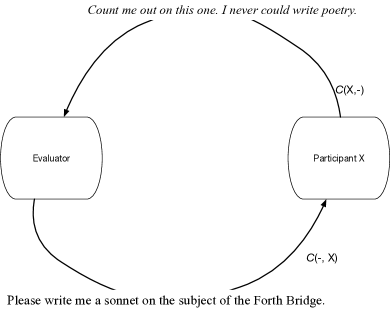
The field of artificial intelligence (AI) has existed for about 7 decades, if we define its origin as beginning with Turing’s famous paper Turing (1950). To answer the question “Can machines think?", Turing suggested it was necessary first to define the words “machine" and “think". He proposed an imitation game, as shown in Figure 1, as a concrete way to frame the problem. Quoting from Turing’s paper:
The new form of the problem can be described in terms of a game which we call the ‘imitation game’.
It is played with three people, a man (A), a woman (B), and an interrogator (C) who may be of either sex. The interrogator stays in a room apart from the other two.
The object of the game for the interrogator is to determine which of the other two is the man and which is the woman. He knows them by labels X and Y, and at the end of the game he says either ‘X is A and Y is B’ or ‘X is B and Y is A’.
Turing proposes replacing one of the human participants with a machine, thereby framing the original question of whether machines can think by the more concrete version of being able to tell from interactions whether one is conversing with a human or a machine:
We now ask the question, ‘What will happen when a machine takes the part of A in this game?’ Will the interrogator decide wrongly as often when the game is played like this as he does when the game is played between a man and a woman? These questions replace our original, ‘Can machines think?’
The imitation game, or what is now more popularly called the Turing Test, has become the mainstay of the field of AI for the ensuing seven decades since Turing wrote his original paper, prompting an immense amount of attention that would be impossible to survey within this paper. The study of imitation games is no longer an academic pursuit: the recent success of generative AI is already being felt in terms of its economic impact around the world. Millions of humans are now playing imitation games with generative AI systems, and there is an alarming increase in the use of “deepfakes" for nefarious purposes. In response, a growing number of software tools are being released that attempt to solve limited classes of imitation games, such as gptzero. 111gptzero can be accessed at https://gptzero.me. We seek to develop a framework for UIGs that applies both to the current generation of generative AI systems being developed on classical computers that are “Turing’s machine" models, as well as the next generation of quantum computers that build on more exotic forms of interaction in braided categories Coecke and Kissinger (2017).
Two recent articles are noteworthy. The first article by Bernardo Goncalves Gonçalves (2024) presents a fascinating historical reconstruction of Turing’s test from archival sources. The second article by Terry Sejnowski Sejnowski (2023) proposes an interesting alternative called a “Reverse Turing Test" based on the recent successes in building large language models (LLMs), which has resulted in possibly the largest ever “natural" experiment conducted on imitation games with literally millions of humans conversing with chatbots like Open AI’s chatGPT. The literature on applications of LLMs is already beyond comprehension, and a review would be impossible here. Adesso (2023) explores how LLMs can shape scientific discovery in the coming decades. Jacques (2023) examines how the teaching of basic computer science will have to be revised in light of the new capabilities of LLMs.
1.2 Universal Imitation Games
Based largely on mathematics developed since Turing – in particular, category theory MacLane (1971) – we investigate a broader class of universal imitation games (UIGs) that captures many other forms of interactions. Category theory is exceptionally well-suited to the study of imitation games as it constitutes a “universal" language for defining interactions: choosing a category means defining a collection of objects and a collection of composable arrows between each pair of objects that represent “measurement probes" for solving UIGs. Figure 2 illustrates our approach to modeling (universal) imitation games, where interactions define contravariant functors or covariant functors , and the solution to an imitation game corresponds to (weak) isomorphism in a category . The Python package DisCoPy de Felice et al. (2021) is a software implementation for computing with string diagrams in category theory, and could be used to implement some of the ideas in this paper. 222Categories for language are described in https://docs.discopy.org/en/main/notebooks/21-05-03-tallcat.html. Toumi (2022) has a detailed description of natural language processing on quantum computers. We will discuss UIGs over quantum computers at the end of the paper in Section 5.
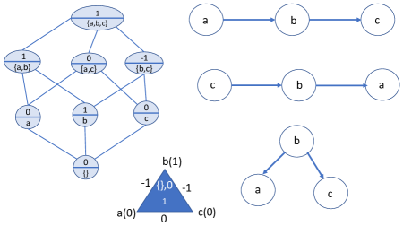
The theoretical foundation of our paper rests on two fundamental insights developed by Yoneda (see Figure 3). The celebrated Yoneda Lemma MacLane (1971) asserts that objects in a category can be defined purely in terms of their interactions with other objects. This interaction is modeled by contravariant or covariant functors:
The Yoneda embedding is sometimes denoted as for the Japanese Hiragana symbol for yo, serves as a universal representer, and generalizes many other similar ideas in machine learning, such as representers in kernel methods Schölkopf and Smola (2002) and representers of causal information Mahadevan (2023). There are many variants of the Yoneda Lemma, including versions that map the functors and into an enriched category. In particular, Bradley et al. (2022a) contains an extended discussion of the use of an enriched Yoneda Lemma to model natural language interactions that result from using a large language model.
The second major insight from Yoneda Yoneda (1960) is based on a powerful concept of the coend and end of a bifunctor that combines both a contravariant and a covariant action. It can be shown that many approaches to solving imitation games, such as building a probabilistic generative model of participants, or using distances in some metric space, correspond to initial or terminal objects in a category of wedges, defined by objects that represent bifunctors, and the arrows are dinatural transformations. These initial or terminal objects correspond to coends and ends. For example, dimensionality reduction methods such as UMAP McInnes et al. (2018) are based mapping a dataset (say of interactions with a participant) into a topological space, which can be shown to define a coend object. Dually, building a probabilistic generative model of a participant essentially defines an end object, as probabilities can be shown to be codensity monads Avery (2016) that are in fact defined by ends. In summary, coends represent geometric ways to solve UIGs, whereas ends represent probabilistic approaches. Bifunctors can be used to construct universal representers of distance functions in generalized metric spaces leading to a “metric Yoneda Lemma" Bonsangue et al. (1998).
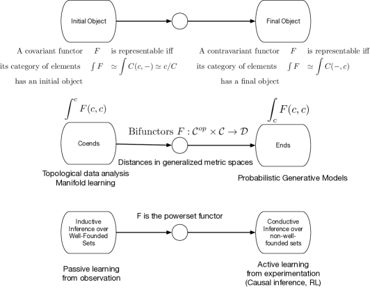

Figure 4 depicts a classification of universal imitation games (UIGs) that will be the primary focus of our paper. In Turing’s original model, discussed above, the participants were assumed to be static, that is, they were not adapting during the course of the interactions. In the case that participants are static, we can try to distinguish between them using a large variety of methods, ranging from distance-based methods like kernel methods Schölkopf and Smola (2002) or optimal transport Villani (2003), or density-based methods such as constructing a generative model. The fundamental ideas developed by Yoneda, in particular Yoneda embeddings and (co)ends play a major role in our paper. For example, Avery (2016) showed that the set of probability distributions on a set can be defined as a codensity monad, which is mathematically equivalent to an end of a bifunctor defined over a functor , where is a category consisting of all convergent sequences with affine maps, and Meas is the category of all measurable spaces. Probabilities are essentially final objects, and in contrast, topological embeddings of the type produced by dimensionality reduction methods like UMAP McInnes et al. (2018) correspond to coends. Another theme of our paper is that we model generative models categorically as universal coalgebras Jacobs (2016); Rutten (2000); Sokolova (2011).
When participants adapt during interactions, we study two special cases: in dynamic UIGs, “learners" imitate “teachers". We contrast the initial object framework of passive learning from observation over well-founded sets using inductive inference – extensively studied by Gold, Solomonoff, Valiant, and Vapnik – with the final object framework of coinductive inference over non-well-founded sets and universal coalgebras, which formalizes learning from active experimentation using causal inference or reinforcement learning. We define a category-theoretic notion of minimum description length or Occam’s razor based on final objects in coalgebras.
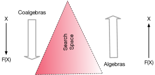
Figure 5 illustrates our study of dynamic UIGs, where “learner" participants are trying to imitate the behavior of “teacher" participants. We contrast two approaches, representing initial and final objects in a category of coalgebras. Induction corresponds to initial algebras over a category defined by the powerset functor over sets. In contrast, coinduction corresponds to final coalgebras. Formally, inductive inference studied by Gold Gold (1967), Solomonoff Solomonoff (1964), Valiant Valiant (1984), and Vapnik Vapnik (1999) corresponds to mathematical induction defined by initial objects over algebras. We contrast inductive inference with coinductive inference in universal coalgebras Aczel (1988); Rutten (2000), which formally corresponds to final objects. Reinforcement learning algorithms, such as TD-learning Sutton and Barto (1998), are typically analyzed as stochastic approximation methods Robbins and Monro (1951); Borkar (2008). In our paper, we model RL in terms of the metric coinduction framework Kozen and Ruozzi (2009) over a coalgebra. The Markov decision process (MDP) model, and its innumerable variants, are all easily modeled as probabilistic coalgebras Sokolova (2011), and the process of TD-learning is essentially a stochastic coinduction inference step towards determining the final coalgebra. This perspective differs considerably from the standard stochastic approximation perspective used to analyze RL algorithms thus far Bertsekas (2022, 2019). The fundamental idea underlying dynamic programming (DP) and reinforcement learning (RL) methds is the Bellman optimality principle, which essentially states that the restriction of any shortest path to a segment must again produce a shortest path, otherwise we can produce a shorter overall path by switching to a shorter segment. This principle is just a special case of the general principle of sheaves, which we discuss in Section 2.7. To the best of our knowledge, the relationship between the Bellman optimality equation and the theory of sheaves MacLane and leke Moerdijk (1994) has not been made before, and represents one of many such examples of the deep insights that come from category-theoretic perspective. Also, by understanding that RL is essentially based on the discovery of final coalgebras in a category of coalgebras, it is possible to explore the vast repertoire of probabilistic coalgebras that have been studied by Sokolova (2011) and others, which may yield many new RL approaches.
Finally, we explore evolutionary UIGs, where a society of participants is playing a large-scale imitation game. Participants in evolutionary UIGs can go extinct from “birth-death" evolutionary processes that model how novel technologies or “mutants" disrupt previously stable equilibria. In the case when the participants are evolving, we introduce the framework of game theory as developed by von Neumann and Morgenstern von Neumann and Morgenstern (1947) and Nash Nash (1951), combined with the use ideas from Darwin’s model of evolution by natural selection. We propose category-theoretic formulations of evolutionary game theory Lieberman et al. (2005).
Figure 2 illustrates a sample of interactions between an evaluator and a participant, with the questions and replies taken from Turing’s original paper Turing (1950). The essence of our paper is to model such interactions by morphisms into and out of an object in a category MacLane (1971). A number of previous studies have explored how natural language can be modeled in terms of objects and morphisms of a category Asudeh and Giorgolo (2020); Bradley et al. (2021); Coecke (2020). At the outset, it is important to clarify that we are proposing a significantly broader vision of imitation games, which we refer to as universal imitation games. More specifically, we are not constraining ourselves to interactions that are purely focused on text, but we include other forms of interaction, including causal experimentation Imbens and Rubin (2015); Pearl (2009), use of machine learning methods more broadly, including distance-based kernel methods Schölkopf and Smola (2002), statistical methods Tibshirani et al. (2010), information theoretic methods Cover and Thomas (2006), inductive inference Gold (1967); Solomonoff (1964), and universal coalgebraic methods that rely on coinduction Jacobs (2016); Rutten (2000). In short, the aim of our framework is to explore the full gamut of approaches available to determine the identity of abstract objects in a category, with a primary goal being its application in AI. To clarify this point further, we view the problem of deciding if a particular image was created by a human or a diffusion based generative AI system Song and Ermon (2019) as an example of an imitation game, or deciding if a particular computer program was written by a human or an AI copilot.
One significant strength of category theory is that it can reveal surprising similarities between algebraic structures that superficially look very different, such as metric spaces and partially ordered sets (see Table 1). A key principle that is often exploited is to explicitly represent the structure in the collection of morphisms between two objects. That is, for some category C, the Hom between objects and might itself have some additional structure beyond that of merely being a collection or a set. For example, in the category of vector spaces, the set of morphisms (linear transformations) between two vector spaces and is itself a vector space. So-called V-enriched categories signify cases when the Hom values are specified in some structure V. Examples include metric spaces, where the Hom values are non-negative real numbers representing distances, and partially ordered sets (posets) where the Hom values are Boolean.
| C | HomC values | Composition and | Domain | Domain for |
|---|---|---|---|---|
| and identity law | for composition | for identity laws | ||
| General category | Sets | Functions | Cartesian product | One element set |
| Metric spaces | Non-negative numbers | sum | zero | |
| Posets | Truth values | Entailment | Conjunction | true |
| V-enriched | objects | morphisms | tensor product | unit object for |
| category | in V | in V | in V | tensor product in V |
| Bivalent functors | Dinatural transformations | Probabilities, distances | Unit object | |
| Coends, ends | topological embeddings |
We view imitation games as fundamental to much of the research in AI in many areas. For example, an autonomous car that is traversing the streets of a busy city like San Francisco is engaged in playing an imitation game at many levels. It has to decide the identity of unknown objects that appear in its perceptual field: is the perceived object a pedestrian or another car? It has to determine its current “state", which could be a complex function of its past observations. Many approaches to modeling state have been studied in the literature, including diversity based representations in automata based on tests Rivest and Schapire (1994), extensions of diversity automata to stochastic sequential models such as partially observable Markov decision processes Singh et al. (2004), coalgebraic notions of state Jacobs (2016), as well as causal experimentation methods Imbens and Rubin (2015). One can view the problem of “black box identification" as containing within it much of the complexity of AI. For example, conversational models involve determining what someone else knows or is thinking about, which involves formal models of knowledge such as modal logic Halpern (2016).
We build on the extensive literature on object isomorphisms in category theory, the bulk of which was developed after Turing’s death in 1954, to formulate universal properties of imitation games, building on the rich mathematical literature on category theory MacLane (1971); Riehl (2017); Richter (2020); Lurie (2009). As we do not assume the prospective reader to have a background in category theory, we have sought to provide a condensed but detailed overview of those parts of category theory that are relevant to formulating UIGs. The aim of category theory is to build a “unified field theory" of mathematics based on a simple model of objects that interact with each other, analogous to directed graph representations. In graphs, vertices represent arbitrary entities, and the edges denote some form of (directional) interaction. In categories, there is no restriction on how many edges exist between any two objects. In a locally small category, there is assumed to be a “set’s worth" of edges, meaning that it could still be infinite! In addition, small categories are assumed to contain a set’s worth of objects (again, which might not be finite). The framework is compositional, in that categories can be formed out of objects, arrows that define the interaction between objects, or functors that define the interactions between categories. This compositionality gives us a rich generative space of models that will be invaluable in modeling UIGs.
We expand on Turing’s concept and analyze a broader class of universal imitation games (UIGs) using mathematics – principally category theory MacLane (1971); Riehl (2017); Richter (2020); Lurie (2009) – that was largely developed after Turing. Category theory gives an exceptional set of “measuring tools" for imitation games. Choosing a category means selecting a collection of objects and a collection of composable arrows by which each pair of objects interact. This choice of objects and arrows defines the measurement apparatus that is used in formulating and solving an imitation game. A key result called the Yoneda Lemma shows that objects can be identified up to isomorphism solely by their interactions with other objects. Category theory also embodies the principle of universality: a property is universal if it defines an initial or final object in a category. Many approaches for solving imitation games, such as probabilistic generative models or distance metrics, can be abstractly characterized as initial or final objects in a category of wedges, where the objects are bifunctors and the arrows are dinatural transformations. Loregian (2021) has an excellent treatment of the calculus of coends, which we will discuss in detail later in the paper.
We classify UIGs into three types: static UIGs, which is closest to Turing’s original formulation, but based on (weak) isomorphism and homotopy; dynamic UIGs, where one participant – the “learner" – is seeking to “imitate" the other participant – a “teacher" – where we contrast the initial object framework of theoretical machine learning defined by inductive inference first studied by Gold and Solomonoff in the 1960s with the dynamical systems final object framework of coinductive inference developed by Aczel and Rutten since the 1980s; and finally evolutionary UIGs, which models a network economy of participants and we analyze the possibility that a new “mutant" can cause the entire economy to imitate it by being better fit. Evolutionary imitation games model both the spread of diseases through a population or the spread of new ideas or technologies that promise investors a better return. We give a category-theoretic model of evolutionary game theory, combining Darwin’s model of evolution by natural selection with the framework of games and economic behavior pioneered by von Neumann, Morgenstern, and Nash.
Abstractly, the problem of solving imitation games can be viewed as comparing two potentially infinitely long strings of tokens that represent the communication from and to the participants. At a high level, our approach builds on the notion of object isomorphism in category theory. We formulate the question of imitation games as deciding if two objects are isomorphic:
Definition 1.
Two objects and in a category are deemed isomorphic, or if and only if there is an invertible morphism , namely is both left invertible using a morphism so that idX, and is right invertible using a morphism where idY.
Category theory provides a rich language to describe how objects interact, including notions like braiding that plays a key role in quantum computing Coecke et al. (2016). The notion of isomorphism can be significantly weakened to include notions like homotopy. This notion of homotopy generalizes the notion of homotopy in topology, which defines why an object like a coffee cup is topologically homotopic to a doughnut (they have the same number of “holes”).
In the category Sets, two finite sets are considered isomorphic if they have the same number of elements, as it is then trivial to define an invertible pair of morphisms between them. In the category Vectk of vector spaces over some field , two objects (vector spaces) are isomorphic if there is a set of invertible linear transformations between them. As we will see below, the passage from a set to the “free” vector space generated by elements of the set is another manifestation of the universal arrow property. In the category of topological spaces Top, two objects are isomorphic if there is a pair of continuous functions that makes them homeomorphic May and Ponto (2012). A more refined category is hTop, the category defined by topological spaces where the arrows are now given by homotopy classes of continuous functions.
Definition 2.
Let and be a pair of objects in a category . We say is a retract of if there exists maps and such that .
Definition 3.
Let be a category. We say a morphism is a retract of another morphism if it is a retract of when viewed as an object of the functor category Hom. A collection of morphisms of is closed under retracts if for every pair of morphisms of , if is a retract of , and is in , then is also in .
The point of these examples is to illustrate that choosing a category, which means choosing a collection of objects and arrows, is like defining a measurement system for deciding if two objects are isomorphic. Thus, in the framework of universal imitation games, as we will show in detail later, there are many choices of categories and each one provides some set of measurement tools. Application areas, like natural language processing or computer vision or robotics, may dictate which set of measurement tools is most appropriate. It is, however, possible to state results that hold regardless of what measurement tools are used (such as the Yoneda Lemma), and we will review the most important of these results for imitation games.
To motivate why homotopy might be useful, a number of recent generative AI systems based on neural or state-space sequence models Gu et al. (2023); Vaswani et al. (2017) enable the summarization of long documents, which can be viewed as compression of a sequence of tokens. In what sense can we determine if the compressed sequence and the original sequence denote the same object? Homotopy provides an answer.
A richer model of interaction is provided by simplicial sets May (1992), which is a graded set , where represents a set of non-interacting objects, represents a set of pairwise interactions, represents a set of three-way interactions, and so on. We can map any category into a simplicial set by constructing sequences of length of composable morphisms. For example, we can model sequences of words in a language as composable morphisms, thereby constructing a simplicial set representation of language-based interactions in an imitation game. Then, the corresponding notion of homotopy between simplicial sets is defined as Richter (2020):
Definition 4.
Let X and Y be simplicial sets, and suppose we are given a pair of morphisms . A homotopy from to is a morphism satisfying and .
These definitions illustrate how category theory can be useful in defining general ways to formulate the problem of imitation games. We now illustrate how category theory is useful in defining generative models that capture much of the work in generative AI, including sequence models.
We expand significantly on Turing’s model of imitation games, which limited itself to static games, to include dynamic imitation games where one participant is a “teacher" and the other is a “learner", as well as evolutionary imitation games, where there is an entire economy of participants that are competing to maximize individual fitness values.
Our core theoretical framework is based defining participants in a UIG as functors that act on categories, collections of objects that interact through arrows or morphisms. To solve Turing’s imitation game, we need to decide if the infinite stream of tokens (e.g., words in a natural language) from two participants in an imitation game (possibly one or both being humans or machines) are “indistinguishable" from each other. Category theory asks whether two objects are isomorphic, not whether they are equal. Accordingly, our formulation of UIGs is based on determining whether two UIG objects are isomorphic, not whether they are equal as Turing originally phrased it. In addition, we can bring to bear the notion of homotopy in category theory Richter (2020); Quillen (1967) and ask if the two participants in a static UIG are homotopic.
Definition 5.
Static UIGs: Given a potentially infinite stream of (multimedia) tokens from and to two participants in an imitation game (see Figure 1), modeled abstractly as objects and in some category , are these two objects (weakly) isomorphic?
In the second type of UIG that we study, it is known that the two participants are in fact different initially from each other. The goal of dynamic UIGs is to determine if asymptotically, the two participants are indistinguishable. This second model captures the process by which generative AI systems are being developed today to pass imitation games, using large language models (LLMs) Vaswani et al. (2017) or through building generative models by diffusion Song and Ermon (2019). An LLM at the beginning outputs random tokens, but over a long process of training on potentially trillions of tokens from datasets like Common Crawl, they appear capable in principle of passing a Turing test.
Definition 6.
Dynamic UIGs: This formulation differs from Turing’s original conception, in that the two participants are known to be different initially, but the question is to determine if asymptotically, the two participants become indistinguishable. That is, given a potentially infinite stream of tokens from the two participants in a dynamic UIG, modeled again as objects and in some category , do these objects become isomorphic in the limit? We can intuitively think of participant as a “teacher" and participant as the “learner" in a dynamic UIG.
Our formulation of dynamic UIGs relates closely to the original theoretical model of inductive inference or language identification in the limit studied by Gold Gold (1967) and Solomonoff Solomonoff (1964), and subsequently refined by many others, incuding Valiant Valiant (1984) and Vapnik Vapnik (1999). We use the mathematics of non-well-founded sets Aczel (1988) and universal coalgebras Jacobs (2016); Rutten (2000) to define a relation called bisimulation to address this problem. We then illustrate how our formulation of dynamic UIGs gives rise to a new framework called coinductive inference for machine learning (ML), and contrast it to the 60-year-old framework of inductive inference proposed by Gold and Solomonoff.
Finally, we explore a third formulation of UIGs termed evolutionary UIGs, combining the principle of evolution by natural selection pioneered by Darwin with the framework of games and economic behavior pioneered by von Neumann and Morgenstern, Nash, and subsequently developed by many others over the past 70 years Maschler et al. (2013). Fundamentally, humans and all other biological organisms on Earth evolved by natural selection, and as the recent Covid-19 pandemic has illustrated, the evolutionary game is one that is indeed a game of the survival of the fittest.
Definition 7.
Evolutionary UIGs: The third formulation differs from the previous two, in that there is a network economy of participants, each of which has a certain fitness to an environment, and the goal is to understand if a particular mutant can cause the entire economy to “imitate" it. Evolutionary UIGs model the spread of diseases through societies, or the spread of new ideas and technologies that promise investors a better return. The problem of evolutionary UIGs is to determine if the economy find an equilibrium point.
Evolutionary UIGs integrates the framework of evolutionary dynamics Lieberman et al. (2005), and non-cooperative games pioneered by Nash Nash (1951). In particular, we focus on identifying fundamental differences between adaptation by incremental processing of experience, as in dynamic UIGs, with the process of random mutation by natural selection, where global changes occur to disrupt an equilibrium. We investigate several models of UIGs, from Valiant’s evolvability Valiant (2009), to birth-death stochastic processes Novak (2006). We give a detailed introduction to variational inequalities (VIs) Facchinei and Pang (2003), which generalize game theory and optimization and illustrate it with an example of playing a generative AI network economy game. We describe a metric coinduction stochastic approximation method for solving VIs Alfredo N. Iusem (2018); Wang and Bertsekas (2015), and outline how to extend such methods to evolutionary UIGs.
The length of this paper is largely due to its tutorial nature, beginning in the next section with a detailed overview of category theory for the reader who may be new to this topic. In Section 2, besides giving a detailed introduction to category theory, we also define several examples of static UIGs. We turn to describe dynamic UIGs in Section 3. Finally, in Section 4, we define evolutionary UIGs.
2 Static Universal Imitation Games: An Introduction to Categories and Functors
In this section, we introduce category theory more formally, and illustrate how it is useful in modeling universal imitation games (UIGs). As noted above, UIGs fundamentally involve determining answering the question Human or Machine?, in the original model that Turing proposed Turing (1950). We propose to generalize this notion in the remainder of this paper, fundamentally starting with our use of category theory, a field of mathematics that has largely developed since Turing. We turn the question posed by Turing into a question of deciding if two objects in a category are (weakly) isomorphic. Thus, in reading this somewhat long section summarizing a lot of work in category theory over the past seven decades, it is useful to keep in mind that at the heart of what we are trying to do is to decide if two participants in a UIG are in some abstract sense “similar" using the various tools provided by category theory. Different categories allow us to “play" the imitation game in various ways, and this chapter is intended to whet the reader’s appetite for the enormous variety of possible ways in which this question can be posed.
Categories are comprised of objects, which can be arbitrarily complex, which gives it an unmatched power of abstraction in virtually all of mathematics MacLane (1971); Riehl (2017); Richter (2020). Categories are compositional structures, and can be built out of smaller category-like objects. Objects in a category interact with each other through arrows or morphisms. One of the most remarkable results in category theory – the Yoneda Lemma – shows that objects in a category can be defined by their interactions. This result forms the underlying motif throughout the rest of this paper, as it relates closely to the problem posed by UIGs. Another central principle in category theory is the notion of a universal property: a property is defined to be universal if it represents an initial or final object in a category. There is a unique arrow from the initial object in a category to every other object. Analogously, there is a unique morphism from every object in the category into the final object. These two special cases illustrate the theme of the Yoneda Lemma of characterizing every object from its interactions. We introduce universal constructions through colimits and limits, pullbacks, equalizers and co-equalizers, which give a rich and flexible way of integrating over objects to find common properties. Functors map one category to another, mapping not just objects, but also the morphisms in a category. Many of the generative models we define in this paper will correspond to functors over some category.
Category theory MacLane (1971); Riehl (2017); MacLane and leke Moerdijk (1994) differs substantially from earlier formulations of AI in terms of causal inference, logic, probability theory, neural networks, statistics, or optimization, all of which essentially can be shown to define special types of categories (e.g., causal models are endofunctors in the category of preorders, probabilities are defined as endofunctors over the category of measurable spaces, optimization methods represent endofunctors over the category of vector spaces, etc). As we will see in the remainder of the paper, many of the theoretical models used in AI can be described in the language of category theory, which provides an unmatched power of abstraction in all of mathematics. It is also singularly suited to modeling computation, and has been extensively explored in other areas of computer science Jacobs (2016).
2.1 Categories and Functors
Table 2 gives a few examples from a myriad of ways in which categories can be defined for formulating UIGs, including approaches based on information theory Baez et al. (2011), statistical methods based on a decomposable probability distribution Pearl (2009), causal methods based on experimentation to test a difference between the participants Pearl (2009); Imbens and Rubin (2015), reinforcement learning methods that are based on modeling the participants as a stochastic dynamical system Sutton and Barto (1998), formal models of knowledge Fagin et al. (1995), universal coalgebraic methods of modeling dynamical systems Jacobs (2016); Rutten (2000), and last but not least, generative AI models based on large language models (LLMs) Vaswani et al. (2017) and diffusion models Song and Ermon (2019).
| Category | Characterization | UIG Application |
|---|---|---|
| Topological spaces | Continuous functions | Analyze document summarization |
| Measurable spaces | Probability monads | Statistical model of participants |
| Coalgebras | , is a functor over sets | Generative AI models |
| Simplicial sets | as objects | Evolutionary UIGs |
| Wedges | Dinatural transformations between | Generalized metric spaces |
| Coends | models topological embeddings | Manifold representations |
| Ends | models integration over measures | Categorical probability |
Category theory is based fundamentally on defining universal properties Riehl (2017), which can be defined as the initial or final object in some category. To take a simple example, the Cartesian product of two sets can be defined as the set of ordered pairs, which tells us what it is, but not what it is good for, or why it is special in some way. Alternatively, we can define the Cartesian product of two sets as an object in the category Sets that has the unique property that every function onto those sets must decompose uniquely as a composition of a function into the Cartesian product object, and then a projection component onto each component set. Furthermore, among all such objects that share this property, the Cartesian product is the final object. In sum, we seek such universal properties that define solutions to imitation games.
We propose a categorical calculus for formulating universal imitation games (UIGs), building on a -year rich legacy of research in AI, mathematics, and computer science. Principally, our framework builds on ideas in category theory that were principally developed since Turing tragically died in 1954 MacLane (1971); MacLane and leke Moerdijk (1994); Riehl (2017); Richter (2020). That very year, Saunders Maclane, a distinguished American mathematician, met with a young Japanese mathematician, Nobuo Yoneda, in the Gare du Nord train station in Paris. That possibly chance encounter led to the development of a profound series of mathematical ideas that revolve around a central core question: can objects can be identified by their interactions with other objects?. The relevance of this question to UIGs is clear, if we abstractly model the participants in a UIG as objects in some category. In a nutshell, our categorical calculus for UIGs posits that two participants in a UIG are indistinguishable if they are isomorphic. One cardinal principle of category theory is to never ask if two objects are equal, only if they are equivalent under a pair of invertible mappings. This categorical perspective succinctly summarizes our formulation of UIGs.
Maclane published a classic textbook on category theory MacLane (1971), where he introduced the mathematical world to the Yoneda Lemma. Our categorical calculus for UIGs builds on the Yoneda Lemma, as well as many ideas that have been developed since, both in category theory Loregian (2021); Richter (2020); Lurie (2009), as well as in theoretical computer science on universal coalgebras Jacobs (2016); Rutten (2000), and the axiomatic foundations of non-well-founded sets Aczel (1988). In 1958, Daniel Kan introduced the concept of adjoint functors, denoted , where the functors and map between two categories and in opposite directions Kan (1958). The fundamental principle here was to note that the collection of interactions between two objects and in a category , denoted variously as , or more simply as was contravariant in the first argument, but covariant in the second argument. It appeared to differ from a tensor product functor that produced a new object , and was covariant in both arguments. As it turned out, both the functor and the tensor product functor were not independent, but formally adjoints of each other. Adjoint functors gives us a further refinement of our categorical calculus for UIGs, since we can now construct functors that map between two apparently dissimilar categories, which may indeed be comparable, such as the category of conditional independence models, modeled as separoids Dawid (2001), and the category of causal models, modeled by an algebraic structure, such as a directed acyclic graph (DAG) Pearl (2009). This relationship was explored previously in Mahadevan (2023) In the context of UIGs, two objects in the category of separoids are only statistically distinguishable, whereas two objects in the causal category of DAG models are causally distinct. By suitably enriching the Hom functor, we can model a rich variety of structures that capture properties of the interactions between two objects and .
Kan also introduced Kan extensions in his paper on adjoint functors, which provide us deeper insight into the study of dynamic UIGs, where initially one participant is a “teacher" and the other is a “learner" that are distinguishable initially, but may become indistinguishable in the limit. (Gold, 1967) proposed the theoretical framework of identification in the limit, motivated by the remarkable ability of human children in acquiring natural language from hearing spoken text. (Solomonoff, 1964) proposed inductive inference as a model for our ability to generalize from examples. Gold’s framework was subsequently elaborated by (Valiant, 1984) and (Vapnik, 1999), based on introducing a probabilistic perspective, as well as introducing the need for efficient estimation with a polynomial number of samples or time. Abstractly, the problem of inductive inference or identification in the limit can be viewed as extrapolating a function from samples of the function. Given a function that is defined on some subset that we want to extend to the entire set , there are no obvious canonical solutions to this problem as it is inherently ill-defined. Much of the work in machine learning over the past six decades has explored various formulations of this function induction problem, usually introducing some regularization principle such as Occam’s Razor, or prefer the simplest hypothesis Belkin et al. (2006), or using some intrinsic measure of the complexity of an object, such as algorithmic information theory Chaitin (2002) based on the shortest program that can generate an object (also referred to as Kolmogorov complexity). In contrast, if instead, we assume that we are extending a functor from some subcategory of a larger category , there are two canonical and “universal" solutions to the functor extension problem given by Kan extensions. Thus, the Kan extension gives us a powerful set of tools to formulate dynamic UIGs.
Yoneda Yoneda (1960) developed another remarkable idea in 1960 based on defining the end of a bifunctor that, like the Hom functor above, is contravariant in the first argument, but covariant in the second argument. The end of a bifunctor refers to an object that represents the terminal object in a category of wedges defined by dinatural transformations between bifunctors . A dual notion is the coend, which represents the initial object. The significance of the end and the coend of a bifunctor to this paper is that they capture universal properties of many AI and ML approaches. In particular, the end can be shown to define the universal property of probability distributions on a space Avery (2016) in terms of the codensity monad, which is defined as the right Kan extension of a functor against itself. Analogously, the coend can be shown to define the topological realization functor of a (fuzzy) simplicial set, which has been the basis for a widely used manifold learning method called UMAP McInnes et al. (2018). A detailed discussion of the calculus of coends is given in Loregian (2021).
Finally, we build on the framework of non-well-founded sets Aczel (1988) and universal coalgebras Jacobs (2016); Rutten (2000) in modeling UIGs. Here, we have a collection of participants that are neither static, nor are they dynamic, but rather they evolve by interacting with each other in a non-cooperative game Maschler et al. (2013). von Neumann and Morgenstern von Neumann and Morgenstern (1947), and subsequently Nash Nash (1951), developed non-cooperative games as a model of economic behavior, which has had a persuasive influence on the development of AI, computer science, and of course, economics. It has also had profound significance in biology in the study of evolutionary games. Our framework builds on the theory of network economics Nagurney (1999), where the participants in an evolutionary UIG are interacting on a graph. The economic activity that occurs in a network economy classifies the participants as producers, such as vendors of generative AI products, transporters who control the network infrastructure over which data is transmitted, and finally consumers who constitute the demand market that must choose between a producer and a transporter. Each participant in an evolutionary UIG is seeking to maximize a selfish goal, and the formulation of evolutionary UIGs is based on determining if the network economy, formulated as a category of coalgebras, has a final coalgebra Rutten (2000).
| Set theory | Category theory |
|---|---|
| set | object |
| subset | subobject |
| truth values | subobject classifier |
| power set | power object |
| bijection | isomorphims |
| injection | monic arrow |
| surjection | epic arrow |
| singleton set | terminal object |
| empty set | initial object |
| elements of a set | morphism |
| - | functors, natural transformations |
| - | limits, colimits, adjunctions |
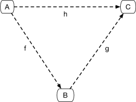
Figure 7 compares the basic notions in set theory vs. category theory. Figure 8 illustrates a simple category of 3 objects: , , and that interact through the morphisms , , and . Categories involve a fundamental notion of composition: the morphism can be defined as the composition of the morphisms from and . What the objects and morphisms represent is arbitrary, and like the canonical directed graph model, this abstractness gives category theory – like graph theory – a universal quality in terms of applicability to a wide range of problems. While categories and graphs and intimately related, in a category, there is no assumption of finiteness in terms of the cardinality of objects or morphisms. A category is defined to be small or locally small if there is a set’s worth of objects and between any two objects, a set’s worth of morphisms, but of course, a set need not be finite. As a simple example, the set of integers defines a category, where each integer is an object and there is a morphism between integers and if . This example serves to immediately clarify an important point: a category is only defined if both the objects and morphisms are defined. The category of integers may be defined in many ways, depending on what the morphisms represent.
Briefly, a category is a collection of objects, and a collection of morphisms between pairs of objects, which are closed under composition, satisfy associativity, and include an identity morphism for every object. For example, sets form a category under the standard morphism of functions. Groups, modules, topological spaces and vector spaces all form categories in their own right, with suitable morphisms (e.g, for groups, we use group homomorphisms, and for vector spaces, we use linear transformations).
A simple way to understand the definition of a category is to view it as a “generalized" graph, where there is no limitation on the number of vertices, or the number of edges between any given pair of vertices. Each vertex defines an object in a category, and each edge is associated with a morphism. The underlying graph induces a “free” category where we consider all possible paths between pairs of vertices (including self-loops) as the set of morphisms between them. In the reverse direction, given a category, we can define a “forgetful” functor that extracts the underlying graph from the category, forgetting the composition rule.
Definition 8.
A graph (sometimes referred to as a quiver) is a labeled directed multi-graph defined by a set of objects, a set of arrows, along with two morphisms and that specify the domain and co-domain of each arrow. In this graph, we define the set of composable pairs of arrows by the set
A category is a graph with two additional functions: , mapping each object to an arrow and , mapping each pair of composable morphisms to their composition .
It is worth emphasizing that no assumption is made here of the finiteness of a graph, either in terms of its associated objects (vertices) or arrows (edges). Indeed, it is entirely reasonable to define categories whose graphs contain an infinite number of edges. A simple example is the group of integers under addition, which can be represented as a single object, denoted and an infinite number of morphisms , each of which represents an integer, where composition of morphisms is defined by addition. In this example, all morphisms are invertible. In a general category with more than one object, a groupoid defines a category all of whose morphisms are invertible. A central principle in category theory is to avoid the use of equality, which is pervasive in mathematics, in favor of a more general notion of isomorphism or weaker versions of it. Many examples of categories can be given that are relevant to specific problems in AI and ML. Some examples of categories of common mathematical structures are illustrated below.
-
•
Set: The canonical example of a category is Set, which has as its objects, sets, and morphisms are functions from one set to another. The Set category will play a central role in our framework, as it is fundamental to the universal representation constructed by Yoneda embeddings.
-
•
Top: The category Top has topological spaces as its objects, and continuous functions as its morphisms. Recall that a topological space consists of a set , and a collection of subsets of closed under finite intersection and arbitrary unions.
-
•
Group: The category Group has groups as its objects, and group homomorphisms as its morphisms.
-
•
Graph: The category Graph has graphs (undirected) as its objects, and graph morphisms (mapping vertices to vertices, preserving adjacency properties) as its morphisms. The category DirGraph has directed graphs as its objects, and the morphisms must now preserve adjacency as defined by a directed edge.
-
•
Poset: The category Poset has partially ordered sets as its objects and order-preserving functions as its morphisms.
-
•
Meas: The category Meas has measurable spaces as its objects and measurable functions as its morphisms. Recall that a measurable space is defined by a set and an associated -field of subsets B that is closed under complementation, and arbitrary unions and intersections, where the empty set .
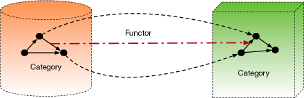
Functors can be viewed as a generalization of the notion of morphisms across algebraic structures, such as groups, vector spaces, and graphs. Functors do more than functions: they not only map objects to objects, but like graph homomorphisms, they need to also map each morphism in the domain category to a corresponding morphism in the co-domain category. Functors come in two varieties, as defined below.
Definition 9.
A covariant functor from category to category , and defined as the following:
-
•
An object (also written as ) of the category for each object in category .
-
•
An arrow in category for every arrow in category .
-
•
The preservation of identity and composition: and for any composable arrows .
Definition 10.
A contravariant functor from category to category is defined exactly like the covariant functor, except all the arrows are reversed.
The functoriality axioms dictate how functors have to be behave:
-
•
For any composable pair in category , .
-
•
For each object in , .
One of the motifs that underlies much of the application of category theory to AI and ML in this paper is to model problems in terms of functors. Figure 9 illustrates the use of functoriality in designing an algorithm for clustering points in a finite metric space based on pairwise distances, one of the most common ways to preprocess data in ML and statistics. Treating clustering as a functor implies the resulting algorithm should behave appropriately under suitable modifications of the input space. Here, we can define clustering formally as a functor that maps the input category of finite metric spaces FinMet defined by , where is a finite set of points in and is a (generalized) finite metric space, and the output category Part is the set of all partitions into subsets such that .
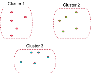
One can impose three criteria on a clustering algorithm, which seem entirely natural, and yet, as Kleinberg Kleinberg (2002) showed, no standard clustering algorithm satisfies all these conditions:
-
•
Scale invariance: If the distance metric is increased or decreased by , where is a scalar real number, the output clustering should not change. In terms of Figure 9, if the points in each cluster became closer together or further apart proportionally, the clustering should remain the same.
-
•
Completeness: For any given partition of the space , there should exist some distance function such that the clustering algorithm when given that distance function should return the desired partition.
-
•
Monotonicity: If the distance between points within each cluster in Figure 9 were decreased, and the distances between points in different clusters were increased, the clustering should not change either.
Remarkably, it turns out that no clustering algorithm exists that satisfies all these three basic conditions. Yet, as Carlsson and Memoli showed Carlsson and Memoli (2010), treating clustering as a functor makes it possible to define a modified clustering problem in terms of creating persistent clusters that overcomes Kleinberg’s impossibility result. This simple but deep example reveals the power of functorial design, and gives a concrete illustration of the importance of categorical thinking in AI and ML.
2.2 Natural Transformations and Universal Arrows
Given any two functors and between the same pair of categories, we can define a mapping between and that is referred to as a natural transformation. These are defined through a collection of mappings, one for each object of , thereby defining a morphism in for each object in .
Definition 11.
Given categories and , and functors , a natural transformation is defined by the following data:
-
•
an arrow in for each object , which together define the components of the natural transformation.
-
•
For each morphism , the following commutative diagram holds true:
A natural isomorphism is a natural transformation in which every component is an isomorphism.
We will see many examples of natural transformations in this paper, but we will use one example here to illustrate its versatility. Figure 10 shows that we can model causal models as functors mapping from an input category of algebraic structures, whose objects represent structural descriptions of the causal model, into an output category of probabilistic representations, whose objects specify the semantics of the causal model.
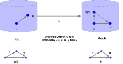
This process of going from a category to its underlying directed graph embodies a fundamental universal construction in category theory, called the universal arrow. It lies at the heart of many useful results, principally the Yoneda lemma that shows how object identity itself emerges from the structure of morphisms that lead into (or out of) it.
Definition 12.
Given a functor between two categories, and an object of category , a universal arrow from to is a pair , where is an object of and is an arrow of , such that the following universal property holds true:
-
•
For every pair with an object of and an arrow of , there is a unique arrow of with .
Definition 13.
If is a category and Set is a set-valued functor, a universal element associated with the functor is a pair consisting of an object and an element such that for every pair with , there is a unique arrow of such that .
Example 1.
Let be an equivalence relation on a set , and consider the quotient set of equivalence classes, where sends each element into its corresponding equivalence class. The set of equivalence classes has the property that any function that respects the equivalence relation can be written as whenever , that is, , where the unique function . Thus, is a universal element for the functor .
Figure 11 illustrates the concept of universal arrows through the connection between categories and graphs. For every (directed) graph , there is a universal arrow from to the “forgetful” functor mapping the category Cat of all categories to Graph, the category of all (directed) graphs, where for any category , its associated graph is defined by . Intuitively, this forgetful functor “throws” away all categorical information, obliterating for example the distinction between the primitive morphisms and vs. their compositions , both of which are simply viewed as edges in the graph . To understand this functor, consider a directed graph defined from a category , forgetting the rule for composition. That is, from the category , which associates to each pair of composable arrows and , the composed arrow , we derive the underlying graph simply by forgetting which edges correspond to elementary arrows, such as or , and which are composites. For example, consider a partial order as the category , and then define as the directed graph that results from the transitive closure of the partial ordering.
The universal arrow from a graph to the forgetful functor is defined as a pair , where is a “universal” graph homomorphism. This arrow possesses the following universal property: for every other pair , where is a category, and is an arbitrary graph homomorphism, there is a functor , which is an arrow in the category Cat of all categories, such that every graph homomorphism uniquely factors through the universal graph homomorphism as the solution to the equation , where (that is, ). Namely, the dotted arrow defines a graph homomorphism that makes the triangle diagram “commute”, and the associated “extension” problem of finding this new graph homomorphism is solved by “lifting” the associated category arrow . This property of universal arrows, as we show in the paper, provide the conceptual underpinnings of universal properties in many applications in AI and ML, as we will see throughout this paper.
2.3 Yoneda lemma and the Universality of Diagrams
The Yoneda Lemma is one of the most celebrated results in category theory, and it provides a concrete example of the power of categorical thinking. Stated in simple terms, it states the mathematical objects are determined (up to isomorphism) by the interactions they make with other objects in a category. We will show the surprising results of applying this lemma to problems involving computing distances between objects in a metric space, reasoning about causal inference, and many other problems of importance in AI and ML. An analogy from particle physics proposed by Theo Johnson-Freyd might help give insight into this remarkable result: “You work at a particle accelerator. You want to understand some particle. All you can do is throw other particles at it and see what happens. If you understand how your mystery particle responds to all possible test particles at all possible test energies, then you know everything there is to know about your mystery particle". The Yoneda Lemma states that the set of all morphisms into an object in a category , denoted as Hom and called the contravariant functor (or presheaf), is sufficient to define up to isomorphism. The category of all presheaves forms a category of functors, and is denoted Set.We will briefly describe two concrete applications of this lemma to two important areas in AI and ML in this section: reasoning about causality and reasoning about distances. The Yoneda lemma plays a crucial role in this paper because it defines the concept of a universal representation in category theory. We first show that associated with universal arrows is the corresponding induced isomorphisms between Hom sets of morphisms in categories. This universal property then leads to the Yoneda lemma.
Theorem 1.
Given any functor , the universal arrow implies a bijection exists between the Hom sets
A special case of this natural transformation that transforms the identity morphism 1r leads us to the Yoneda lemma.
As the two paths shown here must be equal in a commutative diagram, we get the property that a bijection between the Hom sets holds precisely when is a universal arrow from to . Note that for the case when the categories and are small, meaning their Hom collection of arrows forms a set, the induced functor Hom to Set is isomorphic to the functor Hom. This type of isomorphism defines a universal representation, and is at the heart of the causal reproducing property (CRP) defined below.
Lemma 1.
Yoneda lemma: For any functor , whose domain category is “locally small" (meaning that the collection of morphisms between each pair of objects forms a set), any object in , there is a bijection
that defines a natural transformation to the element . This correspondence is natural in both and .
There is of course a dual form of the Yoneda Lemma in terms of the contravariant functor as well using the natural transformation . A very useful way to interpret the Yoneda Lemma is through the notion of universal representability through a covariant or contravariant functor.
Definition 14.
A universal representation of an object in a category is defined as a contravariant functor together with a functorial representation or by a covariant functor together with a representation . The collection of morphisms into an object is called the presheaf, and from the Yoneda Lemma, forms a universal representation of the object.
Later in this Section, we will see how the Yoneda Lemma gives us a novel perspective on causal inference, as well as distance metrics that are at the core of many applications in AI and ML. For causal inference, any causal influence on a variable in a causal model defined as an object in a category must be transmitted through its presheaf. The collection of all such causal influences in effect defines the object itself, giving a more rigorous way to substantiate an observation by the philosopher Plato made more than two millennia ago that
Everything that becomes or changes must do so owing to some cause; for nothing can come to be without a cause Plato (1971)
Another useful concept was introduced by the mathematician Grothendieck, who made many important contributions to category theory.
Definition 15.
The category of elements of a covariant functor is defined as
-
•
a collection of objects where and
-
•
a collection of morphisms for every morphism such that .
Definition 16.
The category of elements of a contravariant functor is defined as
-
•
a collection of objects where and
-
•
a collection of morphisms for every morphism such that .
There is a natural “forgetful" functor that maps the pairs of objects to and maps morphisms to . Below we will show that the category of elements can be defined through a universal construction as the pullback in the diagram of categories.
A key distinguishing feature of category theory is the use of diagrammatic reasoning. However, diagrams are also viewed more abstractly as functors mapping from some indexing category to the actual category. Diagrams are useful in understanding universal constructions, such as limits and colimits of diagrams. To make this somewhat abstract definition concrete, let us look at some simpler examples of universal properties, including co-products and quotients (which in set theory correspond to disjoint unions). Coproducts refer to the universal property of abstracting a group of elements into a larger one.
Before we formally the concept of limit and colimits, we consider some examples. These notions generalize the more familiar notions of Cartesian products and disjoint unions in the category of Sets, the notion of meets and joins in the category Preord of preorders, as well as the least upper bounds and greatest lower bounds in lattices, and many other concrete examples from mathematics.
Example 2.
If we consider a small “discrete” category whose only morphisms are identity arrows, then the colimit of a functor is the categorical coproduct of for , an object of category D, is denoted as
In the special case when the category C is the category Sets, then the colimit of this functor is simply the disjoint union of all the sets that are mapped from objects .
Example 3.
Dual to the notion of colimit of a functor is the notion of limit. Once again, if we consider a small “discrete” category whose only morphisms are identity arrows, then the limit of a functor is the categorical product of for , an object of category D, is denoted as
In the special case when the category C is the category Sets, then the limit of this functor is simply the Cartesian product of all the sets that are mapped from objects .
Category theory relies extensively on universal constructions, which satisfy a universal property. One of the central building blocks is the identification of universal properties through formal diagrams. Before introducing these definitions in their most abstract form, it greatly helps to see some simple examples.
We can illustrate the limits and colimits in diagrams using pullback and pushforward mappings.
An example of a universal construction is given by the above commutative diagram, where the coproduct object uniquely factorizes any mapping , such that any mapping , so that , and furthermore . Co-products are themselves special cases of the more general notion of co-limits. Figure 12 illustrates the fundamental property of a pullback, which along with pushforward, is one of the core ideas in category theory. The pullback square with the objects and implies that the composite mappings must equal . In this example, the morphisms and represent a pullback pair, as they share a common co-domain . The pair of morphisms emanating from define a cone, because the pullback square “commutes” appropriately. Thus, the pullback of the pair of morphisms with the common co-domain is the pair of morphisms with common domain . Furthermore, to satisfy the universal property, given another pair of morphisms with common domain , there must exist another morphism that “factorizes” appropriately, so that the composite morphisms and . Here, and are referred to as cones, where is the limit of the set of all cones “above” . If we reverse arrow directions appropriately, we get the corresponding notion of pushforward. So, in this example, the pair of morphisms that share a common domain represent a pushforward pair. As Figure 12, for any set-valued functor Sets, the Grothendieck category of elements can be shown to be a pullback in the diagram of categories. Here, is the category of pointed sets, and is a projection that sends a pointed set to its underlying set .
We can now proceed to define limits and colimits more generally. We define a diagram of shape in a category formally as a functor . We want to define the somewhat abstract concepts of limits and colimits, which will play a central role in this paper in identifying properties of AI and ML techniques. A convenient way to introduce these concepts is through the use of universal cones that are over and under a diagram.
For any object and any category , the constant functor maps every object of to and every morphism in to the identity morphisms . We can define a constant functor embedding as the collection of constant functors that send each object in to the constant functor at and each morphism to the constant natural transformation, that is, the natural transformation whose every component is defined to be the morphism .
Definition 17.
A cone over a diagram with the summit or apex is a natural transformation whose domain is the constant functor at . The components of the natural transformation can be viewed as its legs. Dually, a cone under with nadir is a natural transformation whose legs are the components .
Cones under a diagram are referred to usually as cocones. Using the concept of cones and cocones, we can now formally define the concept of limits and colimits more precisely.
Definition 18.
For any diagram , there is a functor
which sends to the set of cones over with apex . Using the Yoneda Lemma, a limit of is defined as an object together with a natural transformation , which can be called the universal cone defining the natural isomorphism
Dually, for colimits, we can define a functor
that maps object to the set of cones under with nadir . A colimit of is a representation for . Once again, using the Yoneda Lemma, a colimit is defined by an object together with a natural transformation , which defines the colimit cone as the natural isomorphism
Limit and colimits of diagrams over arbitrary categories can often be reduced to the case of their corresponding diagram properties over sets. One important stepping stone is to understand how functors interact with limits and colimits.
Definition 19.
For any class of diagrams , a functor
-
•
preserves limits if for any diagram and limit cone over , the image of the cone defines a limit cone over the composite diagram .
-
•
reflects limits if for any cone over a diagram whose image upon applying is a limit cone for the diagram is a limit cone over
-
•
creates limits if whenever has a limit in , there is some limit cone over that can be lifted to a limit cone over and moreoever reflects the limits in the class of diagrams.
To interpret these abstract definitions, it helps to concretize them in terms of a specific universal construction, like the pullback defined above in . Specifically, for pullbacks:
-
•
A functor preserves pullbacks if whenever is the pullback of in , it follows that is the pullback of in .
-
•
A functor reflects pullbacks if is the pullback of in whenever is the pullback of in .
-
•
A functor creates pullbacks if there exists some that is the pullback of in whenever there exists a such that is the pullback of in .
Universality of Diagrams
In the category Sets, we know that every object (i.e., a set) can be expressed as a coproduct (i.e., disjoint union) of its elements , where . Note that we can view each element as a morphism from the one-point set to . The categorical generalization of this result is called the density theorem in the theory of sheaves. First, we define the key concept of a comma category.
Definition 20.
Let be a functor from category to . The comma category is one whose objects are pairs , where is an object of and Hom, where is an object of . Morphisms in the comma category from to , where , such that . We can depict this structure through the following commutative diagram:
We first introduce the concept of a dense functor:
Definition 21.
Let D be a small category, C be an arbitrary category, and be a functor. The functor is dense if for all objects of , the natural transformation
is universal in the sense that it induces an isomorphism . Here, is the projection functor from the comma category , defined by .
A fundamental consequence of the category of elements is that every object in the functor category of presheaves, namely contravariant functors from a category into the category of sets, is the colimit of a diagram of representable objects, via the Yoneda lemma. Notice this is a generalized form of the density notion from the category Sets.
Theorem 2.
Universality of Diagrams: In the functor category of presheaves Set, every object is the colimit of a diagram of representable objects, in a canonical way.
Lifting Problems
Lifting problems provide elegant ways to define solutions to computational problems in category theory regarding the existence of mappings. We will use these lifting diagrams later in this paper. For example, the notion of injective and surjective functions, the notion of separation in topology, and many other basic constructs can be formulated as solutions to lifting problems. Lifting problems define ways of decomposing structures into simpler pieces, and putting them back together again.
Definition 22.
Let be a category. A lifting problem in is a commutative diagram in .
Definition 23.
Let be a category. A solution to a lifting problem in is a morphism in satisfying and as indicated in the diagram below.
Definition 24.
Let be a category. If we are given two morphisms and in , we say that has the left lifting property with respect to , or that p has the right lifting property with respect to f if for every pair of morphisms and satisfying the equations , the associated lifting problem indicated in the diagram below.
admits a solution given by the map satisfying and .
Example 4.
Given the paradigmatic non-surjective morphism , any morphism p that has the right lifting property with respect to f is a surjective mapping. .
Example 5.
Given the paradigmatic non-injective morphism , any morphism p that has the right lifting property with respect to f is an injective mapping. .
2.4 Adjoint Functors
Adjoint functors naturally arise in a number of contexts, among the most important being between “free" and “forgetful" functors. Let us consider a canonical example that is of prime significance in many applications in AI and ML.
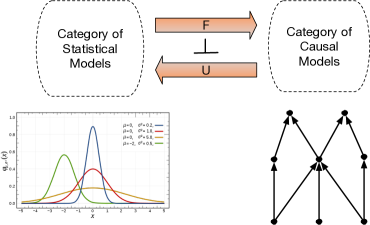
Figure 13 provides a high level overview of the relationship between a category of statistical models and a category of causal models that can be seen as being related by a pair of adjoint “forgetful-free" functors. A statistical model can be abstractly viewed in terms of its conditional independence properties. More concretely, the category of separoids, defined in Section 2, consists of objects called separoids , which are semilattices with a preordering where the elements denote entities in a statistical model. We define a ternary relation , where is interpreted as the statement is conditionally independent of given to denote a relationship between triples that captures abstractly the property that occurs in many applications in AI and ML. For example, in statistical ML, a sufficient statistic of some dataset , treated as a random variable, is defined to be any function for which the conditional independence relationship , where denotes the parameter vector of some statistical model that defines the true distribution of the data. Similarly, in causal inference, denotes a statement about the probabilistic conditional independence of and given . In causal inference, the goal is to recover a partial order defined as a directed acyclic graph (DAG) that ascribes causality among a set of random variables from a dataset specifying a sample of their joint distribution. It is well known that without non-random interventions, causality cannot be inferred uniquely, since because of Bayes rule, there is no way to distinguish causal models such as from the reverse relationship . In both these models, and because of Bayes inversion, one model can be recovered from the other. We can define a “free-forgetful" pair of adjoint functors between the category of conditional independence relationships, as defined by separoid objects, and the category of causal models parameterized by DAG models.
We first review some basic material relating to adjunctions defined by adjoint functors, before proceeding to describe the theory of monads, as the two are intimately related. Our presentation of adjunctions and monads is based on Riehl’s excellent textbook on category theory Riehl (2017) to which the reader is referred to for a more detailed explanation. Adjunctions are defined by an opposing pair of functors that can be defined more precisely as follows.
Definition 25.
An adjunction consists of a pair of functors and , where is often referred to left adjoint and is referred to as the right adjoint, that result in the following isomorphism relationship holding between their following sets of homomorphisms in categories and :
We can express the isomorphism condition more explicitly in the form of the following commutative diagram:
Here, is any morphism in , and denotes the “pullback" of with the mapping to yield the composite mapping . The adjunction condition holds that the transpose of this composite mapping is equal to the composite mapping with . We can express this dually as well, as follows:
where now is a morphism in , and denote the “pushforward" of . Once again, the adjunction condition is a statement that the transpose of the composite mapping is identical to the composite of the mappings with .
It is common to denote adjoint functors in this turnstile notation, indicating that is left adjoint to , or more simply as .
We can use the concept of universal arrows introduced in Section 2 to give more insight into adjoint functors. The adjunction condition for a pair of adjoint functors
implies that for any object , the object represents the functor . Recall from the Yoneda Lemma that the natural isomorphism is determined by an element of , which can be viewed as the transpose of . Denoting such elements as , they can be assembled jointly into the natural transformation . Below we will see that this forms one of the conditions for an endofunctor to define a monad.
Theorem 3.
The unit is a natural transformation defined by an adjunction , whose component is defined to be the transpose of the identity morphism .
Proof: We need to show that for every , the following diagram commutes, which follows from the definition of adjunction and the isomorphism condition that it imposes, as well as the obvious commutativity of the second transposed diagram below the first one.
The dual of the above theorem leads to the second major component of an adjunction.
Theorem 4.
The counit is a natural transformation defined by an adjunction , whose components at is defined to be the transpose of the identity morphism .
Adjoint functors interact with universal constructions, such as limits and colimits, in ways that turn out to be important for a variety of applications in AI and ML. We state the main results here, but refer the reader to Riehl (2017) for detailed proofs. Before getting to the general case, it is illustrative to see the interaction of limits and colimits with adjoint functors for preorders. Recall from above that separoids are defined by a preorder on a join lattice of elements from a set . Given two separoids and , we can define the functors and to be order-preserving functions such that
Such an adjunction between preorders is often called a Galois connection. For preorders, the limit is defined by the meet of the preorder, and the colimit is defined by the join of the preorder. We can now state a useful result. For a fuller discussion of preorders and their applications from a category theory perspective, see Fong and Spivak (2018).
Theorem 5.
Right adjoints preserve meets in a preorder: Let be left adjoint to , where are both preorders, and and are monotone order-preserving functions. For any subset , let . If has a meet , then has a meet , and we can see that , that is, right adjoints preserve meets. Similarly, left adjoints preserve meets, so that if such that then has a join and we can set , so that left adjoints preserve joins.
Proof: The proof is not difficult in this special case of the category being defined as a preorder. If and are monotone adjoint maps on preorders , and is any subset such that its meet is . Since is monotone, , hence it follows that . To show that is the greatest lower bound, if we take any other lower bound , then we want to show that . Since and are adjoint, for every , we have
Hence, for all , which implies is a lower bound for on . Since the meet is the greatest lower bound, we have . Using the Galois connection, we see that , and hence showing that is the greatest lower bound as required. An analogous proof follows to show that left adjoints preserve joins. ∎
We can now state the more general cases for any pair of adjoint functors, as follows.
Theorem 6.
A category admits all limits of diagrams indexed by a small category if and only if the constant functor admits a right adjoint, and admits all colimits of -indexed diagrams if and only if admits a left adjoint.
By way of explanation, the constant functor sends every object of to and every morphism of to the identity morphism . Here, the constant functor sends every object of to the constant diagram , namely the functor that maps each object of to the object and each morphism of to the identity . The theorem follows from the definition of the universal properties of colimits and limits. Given any object , and any diagram (functor) , the set of morphisms corresponds to the set of natural transformations from the constant -diagram at to the diagram . These natural transformations precisely correspond to the cones over with summit in the definition given earlier in Section 2. It follows that there is an object together with an isomorphism
We can now state the more general result that we showed above for the special case of adjoint functors on preorders.
Theorem 7.
Right adjoints preserve limits, whereas left adjoints preserve colimits.
2.5 Ends, Coends, and Kan Extensions
Perhaps the most canonical category for formulating UIGs is the category of wedges, which are defined by a collection of objects comprised of bifunctors , and a collection of arrows between each pair of bifunctors called a dinatural transformation (as an abbreviation for diagonal natural transformation). We will see below that the initial and terminal objects in the category of wedges correspond to a beatiful idea first articulated by Yoneda called the coend or end Yoneda (1960). Loregian (2021) has an excellent treatment of coend calculus, which we will use below.
Definition 26.
Given a pair of bifunctors , a dinatural transformation is defined as follows:
As Loregian (2021) observes, just as a natural transformation interpolates between two regular functors and by filling in the gap between their action on a morphism and on the codomain category, a dinatural transformation “fills in the gap" between the top of the hexagon above and the bottom of the hexagon.
We can define a constant bifunctor by the object it maps everything to, namely the input pair of objects are both mapped to the object , and the two input morphisms are both mapped to the identity morphism on . We can now define wedges and cowedges.
Definition 27.
A wedge for a bifunctor is a dinatural transformation from the constant functor on the object to . Dually, we can define a cowedge for a bifunctor by the dinatural transformation .
We can now define a category of wedges, each of whose objects are wedges, and for arrows, we choose arrows in the co-domain category that makes the diagram below commute.
Definition 28.
Given a fixed bifunctor , we define the category of wedges where each object is a wedge and given a pair of wedges and , we choose an arrow that makes the following diagram commute:
Analogously, we can define a category of cowedges where each object is defined as a cowedge .
With these definitions in place, we can once again define the universal property in terms of initial and terminal objects. In the category of wedges and cowedges, these have special significance for formulating and solving UIGs, as we will see in the next section.
Definition 29.
Given a bifunctor , the end of consists of a terminal wedge . The object is itself called the end. Dually, the coend of is the initial object in the category of cowedges , where the object is itself called the coend of .
Remarkably, probabilities can be formally shown to define ends of a category Avery (2016), and topological embeddings of datasets, as implemented in popular dimensionality reduction methods like UMAP McInnes et al. (2018), correspond to coends MacLane (1971). These connections suggest the canonical importance of the category of wedges and cowedges in formulating and solving UIGs. First, we introduce another universal construction, the Kan extension, which turns out to be the basis of every other concept in category theory.
Extending Functors rather than Functions: Kan Extensions
Often, in machine learning, we are given samples of a function defined on some subset and we want to extend the function over a larger set , but there is no obvious or canonical extension of functions. This ill-defined nature of machine learning has prompted a large variety of solutions, such as regularization or Occam’s razor (prefer the simplest function). In contrast, if we are given a functor , and we want to extend the functor to a larger category , there are only two canonical solutions that present themselves. These are referred to as the Kan extensions. There is a close connection between the notions of ends and coends and Kan extensions Loregian (2021), as well as to the categorical foundation of probability Avery (2016).
Definition 30.
A left Kan extension of a functor along another functor , is a functor with a natural transformation such that for any other such pair , factors uniquely through . In other words, there is a unique natural transformation .
Definition 31.
A right Kan extension of a functor along another functor , is a functor with a natural transformation such that for any other such pair , factors uniquely through . In other words, there is a unique natural transformation .
2.6 Monads and Categorical Probability
Now, we turn to defining monads more formally, and relate them to adjoint functors. Categorically speaking, probabilities are essentially monads Avery (2016); Giry (1982). Like the case with coalgebras, which we discussed extensively in previous Sections, monads also are defined by an endofunctor on a category, but one that has some special properties. These additional properties make monads possess algebraic structure, which leads to many interesting properties. Monads provide a categorical foundation for probability, based on the property that the set of all distributions on a measurable space is itself a measurable space Avery (2016). The well-known Giry monad Giry (1982) been also shown to arise as the codensity monad of a forgetful functor from the category of convex sets with affine maps to the category of measurable spaces Avery (2016). Our goal in this paper is to apply monads to shed light into causal inference. We first review the basic definitions of monads, and then discuss monad algebras, which provide ways of characterizing categories.
Consider the pair of adjoint free and forgetful functors between graphs and categories. Here, the domain category is Cat, the category of all categories whose objects are categories and whose morphisms are functors. The co-domain category is the category Graph of all graphs, whose objects are directed graphs, and whose morphisms are graph homomorphisms. Here, a monad is induced by composing the “free" functor that maps a graph into its associated “free" category, and the “forgetful" functor that maps a category into its associated graph. The monad in effect takes a directed graph and computes its transitive closure . More precisely, for every (directed) graph , there is a universal arrow from to the “forgetful" functor mapping the category Cat of all categories to Graph, the category of all (directed) graphs, where for any category , its associated graph is defined by .
To understand this functor, simply consider a directed graph as a category forgetting the rule for composition. That is, from the category , which associates to each pair of composable arrows and , the composed arrow , we derive the underlying graph simply by forgetting which edges correspond to elementary functions, such as or , and which are composites. The universal arrow from a graph to the forgetful functor is defined as a pair , where is a a graph homomorphism. This arrow possesses the following universal property: for every other pair , where is a category, and is an arbitrary graph homomorphism, there is a functor , which is an arrow in the category Cat of all categories, such that every graph homomorphism uniquely factors through the universal graph homomorphism as the solution to the equation , where (that is, ). Namely, the dotted arrow defines a graph homomorphism that makes the triangle diagram “commute", and the associated “extension" problem of finding this new graph homomorphism is solved by “lifting" the associated category arrow . In causal inference using graph-based models, the transitive closure graph is quite important in a number of situations. It can be the initial target of a causal discovery algorithm that uses conditional independence oracles. It is also common in graph-based causal inference Pearl (2009) to model causal effects through a directed acyclic graph (DAG) , which specifies its algebraic structure, and through a set of probability distributions on that specifies its semantics . Often, reasoning about causality in a DAG requires examining paths that lead from some vertex , representing a causal variable, to some other vertex . The process of constructing the transitive closure of a DAG provides a simple example of a causal monad.
Definition 32.
A monad on a category consists of
-
•
An endofunctor
-
•
A unit natural transformation
-
•
A multiplication natural transformation
such that the following commutative diagram in the category commutes (notice the arrows in this diagram are natural transformations as each object in the diagram is a functor).
It is useful to think of monads as the “shadow" cast by an adjunction on the category corresponding to the co-domain of the right adjoint . Consider the following pair of adjoint functors .
In the language of ML, if we treat category as representing “labeled training data" where we have full information, and category as representing a new domain for which we have no labels, what can we conclude about category from the information we have from the adjunction? The endofunctor on is of course available to us, as is the natural transformation . The map for any object is an endofunctor on , about which we have no information. However, the augmented natural transformation can be studied in category . From this data, what can we conclude about the objects in category ? In response to the natural question of whether every monad can be defined by a pair of adjoint functors, two solutions arose that came about from two different pairs of adjoint functors. These are referred to as the Eilenberg-Moore category and the Kleisli category MacLane (1971).
Codensity Monads and Probability
A striking recent finding is that categorical probability structures, such as Giry monads, are in essence codensity monads that result from extending a certain functor along itself Avery (2016).
Definition 33.
A codensity monad of a functor is the right Kan extension of along itself (if it exists). The codensity monad inherits the university property from the Kan extension.
Codensity monads can also be written using Yoneda’s abstract integral calculus as ends:
Here, the notation , where is any set, and is any object of a category , denotes the product in of copies of .
Definition 34.
A convex set is a convex subset of a real vector space, where for all , and for all , the convex combination . An affine map is a function such that where .
To define categorical probability as codensity monads, we need to define forgetful functors from the category of compact convex subsets of with affine maps to the category of measurable spaces and measurable functions. In addition, let be the category with the object adjoined, where is the convex set of convergent sequences in the unit interval .
Theorem 8.
Avery (2016) The be the category of compact convex subsets of for varying with affine maps between them, and let be the same with the object adjoined. Then, the codensity monads of the forgetful functors and are the finitely additive Giry monad and the Giry monad respectively.
The well-known Giry monad Giry (1982) defines probabilities in both the discrete case and the continuous case (over Polish spaces) in terms of endofunctor on the category of measurable spaces .
2.7 Sheaves and Topoi
In this section, we define an important categorical structure defined by sheaves and topoi MacLane and leke Moerdijk (1994). Yoneda embeddings define (pre)sheaves, which satisfy a number of crucial properties that make it remarkably similar to the category of Sets. The sheaf condition plays an important role in many applications of machine learning, from dimensionality reduction McInnes et al. (2018) to causal inference Mahadevan (2023). MacLane and leke Moerdijk (1994) provides an excellent overview of sheaves and topoi, and how remarkably they unify much of mathematics, from geometry to logic and topology. We will give only the briefest of overviews here, and apply in the main ideas to the study of UIGs.
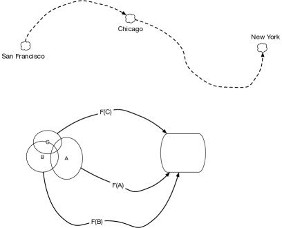
Figure 14 gives two concrete examples of sheaves. In a minimum cost transportation problem, say using optimal transport Villani (2003) or reinforcement learning Sutton and Barto (1998), any optimal solution has the property that any restriction of the solution must also be optimal. In RL, this sheaf principle is codified by the Bellman equation, and leads to the fundamental principle of dynamic programming Bertsekas (2005). Consider routing candy bars from San Francisco to New York city. If the cheapest way to route candy bars is through Chicago, then the restriction of the overall route to the (sub) route from Chicago to New York City must also be optimal, otherwise it is possible to find a shortest overall route by switching to a lower cost route. Similarly, in function approximation with real-valued functions , where is the category of topological spaces, the (sub)functions and restricted to the open sets , and must agree on the values they map the elements in the intersections , , and so on. Similarly, in causal inference, any probability distribution that is defined over a causal model must satisfy the sheaf condition in that any restriction of the causal model to a submodel must be consistent, so that two causal submodels that overlap in their domains must agree on the common elements.
Sheaves can be defined over arbitrary categories, and we introduce the main idea by focusing on the category of sheaves over Sets.
Definition 35.
MacLane and leke Moerdijk (1994) A sheaf of sets on a topological space is a functor such that each open covering of an open set of yields an equalizer diagram
The above definition succinctly captures what Figure 14 shows for the example of approximating functions: the value of each subfunction must be consistent over the shared elements in the intersection of each open set.
Definition 36.
The category of sheaves over a space is a full subcategory of the functor category .
Grothendieck Topologies
We can generalize the notion of sheaves to arbitrary categories using the Yoneda embedding . We explain this generalization in the context of a more abstract topology on categories called the Grothendieck topology defined by sieves. A sieve can be viewed as a subobject in the presheaf , but we can define it more elegantly as a family of morphisms in , all with codomain such that
Figure 15 illustrates the idea of sieves. A simple way to think of a sieve is as a right ideal. We can define that more formally as follows:
Definition 37.
If is a sieve on , and is any arrow in category , then
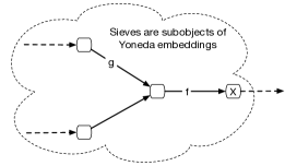
Definition 38.
MacLane and leke Moerdijk (1994) A Grothendieck topology on a category is a function which assigns to each object of a collection of sieves on such that
-
1.
the maximum sieve is in .
-
2.
If then for any arrow .
-
3.
If and is any sieve on , such that for all , then .
We can now define categories with a given Grothendieck topology as sites.
Definition 39.
A site is defined as a pair consisting of a small category and a Grothendieck topology on .
An intuitive way to interpret a site is as a generalization of the notion of a topology on a space , which is defined as a set together with a collection of open sets . The sieves on a category play the role of “open sets".
Exponential Objects and Cartesian Closed Categories
To define a topos, we need to understand the category of Sets a bit more. Clearly, the single point set is a terminal object for Sets, and the binary product of two sets can always be defined. Furthermore, given two sets and , we can define as the exponential object representing the set of all functions . We can define exponential objects in any category more generally as follows.
Definition 40.
Given any category with products, for a fixed object in , we can define the functor
If this functor has a right adjoint, which can be denoted as
then we say is an exponentiable object of .
Definition 41.
A category is Cartesian closed if it has finite products (which is equivalent to saying it has a terminal object and binary products) and if all objects in are exponentiable.
A result that is of foundational importance to this paper is that the category defined by Yoneda embeddings is Cartesian closed.
Theorem 9.
MacLane and leke Moerdijk (1994) For any small category , the functor category is Cartesian closed
For a detailed proof, the reader is referred to MacLane and leke Moerdijk (1994). A further result of significance is the density theorem, which can be seen as the generalization of the simple result that any set can be defined as the union of single point sets .
Theorem 10.
MacLane and leke Moerdijk (1994) In a functor category , any object is the colimit of a diagram of representable objects in a canonical way.
Subobject Classifiers
A topos builds on the property of subobject classifiers in Sets. Given any subset , we can define as the monic arrow defined by the inclusion of in , or as the characteristic function that is equal to for all elements that belong to , and takes the value otherwise. We can define the set and treat true as the inclusion in . The characteristic function can then be defined as the pullback of true along .
We can now define subobject classifiers in a category as follows.
Definition 42.
In a category with finite limits, a subobject classifier is a monic arrow , such that to every other monic arrow in , there is a unique arrow that forms the following pullback square:
This definition can be rephrased as saying that the subobject functor is representable. In other words, a subobject of an object in a category is an equivalence class of monic arrows .
Heyting Algebras
A truly remarkable finding is that the logic of topoi is not classical Boolean logic, but intuitionistic logic defined by Heyting algebras.
Definition 43.
A Heyting algebra is a poset with all finite products and coproducts, which is Cartesian closed. That is, a Heyting algebra is a lattice with and which has to each pair of elements and an exponential . The exponential is written , and defined as the adjunction
Alternatively, is a least upper bound for all those elements with . Therefore, for the particular case of , we get that . In the figure below, the arrows show the partial ordering relationship. As a concrete example, for a topological space the set of open setx is a Heyting algebra. The binary intersections and unions of open sets yield open sets. The empty set represents and the complete set represents . Given any two open sets and , the exponential object is defined as the union of all open sets for which .
Note that in a Boolean algebra, we define implication as the relationship
This property, which is sometimes referred to as the “law of the excluded middle" (because if , then this translates to ), does not hold in a Heyting algebra. For example, on a real line , if we define the open sets by the open intervals , the complement of an open set need not be open.
We can now state what is a truly remarkable result about the subobjects of a (pre)sheaf.
Theorem 11.
MacLane and leke Moerdijk (1994) For any functor category of a small category , the partially ordered set of subobjects of , for any object of is a Heyting algebra.
This result has deep implications for a lot of applications in AI and ML that are based modeling presheaves, including causal inference and decision making. It implies that the proper logic to employ in these settings is intuitionistic logic, not classical logic as is often used in AI Pearl (2009); Fagin et al. (1995); Halpern (2016).
Finally, we can now define the category of topoi.
Definition 44.
A topos is a category with
-
1.
A pullback for every diagram .
-
2.
A terminal object .
-
3.
An object and a monic arrow such that any monic , there is a unique arrow in for which the following square is a pullback:
-
4.
To each object an object and an arrow such that for every arrow , there is a unique arrow for which the following diagrams commute:
2.8 Higher-Order Categories
Simplicial sets are higher-dimensional generalizations of directed graphs, partially ordered sets, as well as regular categories themselves. Importantly, simplicial sets and simplicial objects form a foundation for higher-order category theory. Simplicial objects have long been a foundation for algebraic topology, and more recently in higher-order category theory. The category has non-empty ordinals as objects, and order-preserving maps as arrows. An important property in is that any many-to-many mapping is decomposable as a composition of an injective and a surjective mapping, each of which is decomposable into a sequence of elementary injections , called coface mappings, which omits , and a sequence of elementary surjections , called co-degeneracy mappings, which repeats . The fundamental simplex is the presheaf of all morphisms into , that is, the representable functor . The Yoneda Lemma assures us that an -simplex can be identified with the corresponding map . Every morphism in is functorially mapped to the map in .
Any morphism in the category can be defined as a sequence of co-degeneracy and co-face operators, where the co-face operator is defined as:
Analogously, the co-degeneracy operator is defined as
Note that under the contravariant mappings, co-face mappings turn into face mappings, and co-degeneracy mappings turn into degeneracy mappings. That is, for any simplicial object (or set) , we have , and likewise, .
Example 6.
The “vertices” of a simplicial object are the objects in , and the “edges” of are its arrows , where and are objects in . Given any such arrow, the degeneracy operators and recover the source and target of each arrow. Also, given an object of category , we can regard the face operator as its identity morphism .
Example 7.
Given a category , we can identify an -simplex of a simplicial set with the sequence:
the face operator applied to yields the sequence
where the object is “deleted” along with the morphism leaving it.
Example 8.
Given a category , and an -simplex of the simplicial set , the face operator applied to yields the sequence
where the object is “deleted” along with the morphism entering it. Note this face operator can be viewed as analogous to interventions on leaf nodes in a causal DAG model.
Example 9.
Given a category , and an -simplex of the simplicial set the face operator applied to yields the sequence
where the object is “deleted” and the morphisms is composed with morphism . Note that this process can be abstractly viewed as intervening on object by choosing a specific value for it (which essentially “freezes” the morphism entering object to a constant value).
Example 10.
Given a category , and an -simplex of the simplicial set , the degeneracy operator applied to yields the sequence
where the object is “repeated” by inserting its identity morphism .
Definition 45.
Given a category , and an -simplex of the simplicial set , is a degenerate simplex if some in is an identity morphism, in which case and are equal.
Simplicial Subsets and Horns
We now describe more complex ways of extracting parts of categorical structures using simplicial subsets and horns. These structures will play a key role in defining suitable lifting problems.
Definition 46.
The standard simplex is the simplicial set defined by the construction
By convention, . The standard -simplex maps each to the single element set .
Definition 47.
Let denote a simplicial set. If for every integer , we are given a subset , such that the face and degeneracy maps
applied to result in
then the collection defines a simplicial subset
Definition 48.
The boundary is a simplicial set Set defined as
Note that the boundary is a simplicial subset of the standard -simplex .
Definition 49.
The Horn Set is defined as
Intuitively, the Horn can be viewed as the simplicial subset that results from removing the interior of the -simplex together with the face opposite its th vertex.
Consider the problem of composing -dimensional simplices to form a -dimensional simplicial object. Each simplicial subset of an -simplex induces a a horn , where . Intuitively, a horn is a subset of a simplicial object that results from removing the interior of the -simplex and the face opposite the th vertex. Consider the three horns defined below. The dashed arrow indicates edges of the -simplex not contained in the horns.
The inner horn is the middle diagram above, and admits an easy solution to the “horn filling” problem of composing the simplicial subsets. The two outer horns on either end pose a more difficult challenge. For example, filling the outer horn when the morphism between and is and that between and is the identity is tantamount to finding the left inverse of up to homotopy. Dually, in this case, filling the outer horn is tantamount to finding the right inverse of up to homotopy. A considerable elaboration of the theoretical machinery in category theory is required to describe the various solutions proposed, which led to different ways of defining higher-order category theory Boardman and Vogt (1973); Joyal (2002); Lurie (2009).
Higher-Order Categories
We now formally introduce higher-order categories, building on the framework proposed in a number of formalisms. We briefly summarize various approaches to the horn filling problem in higher-order category theory.
Definition 50.
Let be a morphism of simplicial sets. We say is a Kan fibration if, for each , and each , every lifting problem.
admits a solution. More precisely, for every map of simplicial sets and every -simplex extending , we can extend to an -simplex satisfying .
Example 11.
Given a simplicial set , then a projection map that is a Kan fibration is called a Kan complex.
Example 12.
Any isomorphism between simplicial sets is a Kan fibration.
Example 13.
The collection of Kan fibrations is closed under retracts.
Definition 51.
Lurie (2009) An -category is a simplicial object which satisfies the following condition:
-
•
For , every map of simplicial sets can be extended to a map .
This definition emerges out of a common generalization of two other conditions on a simplicial set :
-
1.
Property K: For and , every map of simplicial sets can be extended to a map .
-
2.
Property C: for , every map of simplicial sets can be extended uniquely to a map .
Simplicial objects that satisfy property K were defined above to be Kan complexes. Simplicial objects that satisfy property C above can be identified with the nerve of a category, which yields a full and faithful embedding of a category in the category of sets. definition 51 generalizes both of these definitions, and was called a quasicategory in Joyal (2002) and weak Kan complexes in Boardman and Vogt (1973) when is a category. We will use the nerve of a category below in defining homotopy colimits as a way of characterizing a causal model.
Example: Simplicial Objects over Causal String Diagrams
We now illustrate the above formalism of simplicial objects by illustrating how it applies to the special case where causal models are defined over symmetric monoidal categories Fong (2012); Jacobs et al. (2019); Fritz and Klingler (2023). For a detailed overview of symmetric monoidal categories, we recommend the book-length treatment by Fong and Spivak (2018). Symmetric monoidal categories (SMCs) are useful in modeling processes where objects can be combined together to give rise to new objects, or where objects disappear. For example, Coecke et al. (2016) propose a mathematical framework for resources based on SMCs. We focus on the work of Jacobs et al. (2019). It is important to point out that monoidal categories can be defined as a special type of Grothendieck fibration Richter (2020). We discuss one specific case of the general Grothendieck construction in the next section construction, and refer the reader to Richter (2020) for how the structure of monoidal categories itself emerges from this construction.
Our goal in this section is to illustrate how we can define simplicial objects over the SMC category CDU category SynG constructed by Jacobs et al. (2019) to mimic the process of working with an actual Bayesian network DAG For the purposes of our illustration, it is not important to discuss the intricacies involved in this model, for which we refer the reader to the original paper. In particular, we can solve an associated lifting problem that is defined by the functor mapping the simplicial category to their SMC category. They use the category of stochastic matrices to capture the process of working with the joint distribution as shown in the figure. Instead, one can use some other category, such as the category of Sets, or Top (the category of topological spaces), or indeed, the category Meas of measurable spaces.
Recall that Bayesian networks Pearl (2009) define a joint probability distribution
where represents a subset of variables (not including the variable itself). Jacobs et al. (2019) show Bayesian network models can be constructed using symmetric monoidal categories, where the tensor product operation is used to combine multiple variables into a “tensored” variable that then probabilistically maps into an output variable. In particular, the monoidal category Stoch has as objects finite sets, and morphisms are dimensional stochastic matrices. Composition of stochastic matrices corresponds to matrix multiplication. The monoidal product in Stoch is the cartesian product of objects, and the Kronecker product of matrices . Jacobs et al. (2019) define three additional operations, the copy map, the discarding map, and the uniform state.
Definition 52.
A CDU category (for copy, discard, and uniform) is a SMC category (C, , ), where each object has a copy map , and discarding map , and a uniform state map , satisfying a set of equations detailed in Jacobs et al. (2019). CDU functors are symmetric monoidal functors between CDU categories, preserving the CDU maps.
The key theorem we are interested in is the following from the original paper Jacobs et al. (2019):
Theorem 12.
There is an isomorphism (1-1 correspondence) between Bayesian networks based on a DAG and CDU functors Syn Stoch.
Nerve of a Category
The nerve of a category enables embedding into the category of simplicial objects, which is a fully faithful embedding Lurie (2009); Richter (2020).
Definition 53.
Let be a functor from category to category . If for all arrows the mapping
-
•
injective, then the functor is defined to be faithful.
-
•
surjective, then the functor is defined to be full.
-
•
bijective, then the functor is defined to be fully faithful.
Definition 54.
The nerve of a category is the set of composable morphisms of length , for . Let denote the set of sequences of composable morphisms of length .
The set of -tuples of composable arrows in C, denoted by , can be viewed as a functor from the simplicial object to . Note that any nondecreasing map determines a map of sets . The nerve of a category C is the simplicial set , which maps the ordinal number object to the set .
The importance of the nerve of a category comes from a key result Richter (2020), showing it defines a full and faithful embedding of a category:
Theorem 13.
The nerve functor Cat Set is fully faithful. More specifically, there is a bijection defined as:
Using this concept of a nerve of a category, we can now state a theorem that shows it is possible to easily embed the CDU symmetric monoidal category defined above that represents Bayesian Networks and their associated “string diagram surgery” operations for causal inference as a simplicial set.
Theorem 14.
Define the nerve of the CDU symmetric monoidal category (C, , ), where each object has a copy map , and discarding map , and a uniform state map as the set of composable morphisms of length , for . Let denote the set of sequences of composable morphisms of length .
The associated nerve functor Cat Set from the CDU category is fully faithful. More specifically, there is a bijection defined as:
This theorem is just a special case of the above theorem attesting to the full and faithful embedding of any category using its nerve, which then makes it a simplicial set. We can then use the theoretical machinery at the top layer of the UCLA architecture to manipulate causal interventions in this category using face and degeneracy operators as defined above.
Note that the functor from a simplicial object to a category can be lossy. For example, we can define the objects of to be the elements of , and the morphisms of as the elements , where , and , and , and as defining the identity morphisms . Composition in this case can be defined as the free algebra defined over elements of , subject to the constraints given by elements of . For example, if , we can impose the requirement that . Such a definition of the left adjoint would be quite lossy because it only preserves the structure of the simplicial object up to the -simplices. The right adjoint from a category to its associated simplicial object, in contrast, constructs a full and faithful embedding of a category into a simplicial set. In particular, the nerve of a category is such a right adjoint.
Topological Embedding of Simplicial Sets
Simplicial sets can be embedded in a topological space using coends MacLane (1971), which is the basis for a popular machine learning method for reducing the dimensionality of data called UMAP (Uniform Manifold Approximation and Projection) McInnes et al. (2018).
Definition 55.
The geometric realization of a simplicial set is defined as the topological space
where the -simplex is assumed to have a discrete topology (i.e., all subsets of are open sets), and denotes the topological -simplex
The spaces can be viewed as cosimplicial topological spaces with the following degeneracy and face maps:
Note that , whereas .
The equivalence relation above that defines the quotient space is given as:
Topological Embeddings as Coends
We now bring in the perspective that topological embeddings can be interpreted as coends as well. Consider the functor
where
where acts contravariantly as a functor from to mapping , and covariantly mapping as a functor from to the category Top of topological spaces.
2.9 Homotopy in Categories
To motivate the need to consider homotopical equivalence, we consider the following problem: a generative AI system can be used to construct summaries of documents, which raises the question of how to decide if a document summary reflects the actual document. If we view a document as an object in a category, then the question becomes one of deciding object equivalence in a looser sense of homotopy, namely is there an invertible transformation between the original document and its summary? We discuss how to construct the topological embedding of an arbitrary category by embedding it into a simplicial set by constructing its nerve, and then finding the topological embedding of the nerve using the homotopy colimit Richter (2020). First, we discuss the topological embedding of a simplicial set, and formulate it in terms of computing a coend. As another example, causal models can only be determined up to some equivalence class from data, and while many causal discovery algorithms assume arbitrary interventions can be carried out to discover the unique structure, such interventions are generally impossible to do in practical applications. The concept of essential graph Andersson et al. (1997) is based on defining a “quotient space” of graphs, but similar issues arise more generally for non-graph based models as well. Thus, it is useful to understand how to formulate the notion of equivalent classes of causal models in an arbitrary category. For example, given the conditional independence structure , there are at least three different symmetric monoidal categorical representations that all satisfy this conditional independence Fong (2012); Jacobs et al. (2019); Fritz and Klingler (2023), and we need to define the quotient space over all such equivalent categories.
In our previous work on causal homotopy Mahadevan (2021a), we exploited the connection between causal DAG graphical models and finite topological spaces. In particular, for a DAG model , it is possible to define a finite space topology , whose open sets are subsets of the vertices such that each vertex is associated with an open set defined as the intersection of all open sets that contain . This structure is referred to an Alexandroff topology, which can be shown to emerge from universal representers defined by Yoneda embeddings in generalized metric spaces. An intuitive way to construct an Alexandroff topology is to define the open set for each variable by the set of its ancestors , or by the set of its descendants . This approach transcribes a DAG graph into a finite topological space, upon which the mathematical tools of algebraic topology can be applied to construct homotopies among equivalent causal models. Our approach below generalizes this construction to simplicial objects, as well as general categories.
The Category of Fractions: Localizing Invertible Morphisms in a Category
One way to pose the question of homotopy is to ask whether a category can be reduced in some way such that all invertible morphisms can be “localized" in some way. The problem of defining a category with a given subclass of invertible morphisms, called the category of fractions (Gabriel et al., 1967), is another concrete illustration of the close relationships between categories and graphs. Borceux (1994) has a detailed discussion of the “calculus of fractions”, namely how to define a category where a subclass of morphisms are to be treated as isomorphisms. The formal definition is as follows:
Definition 56.
Consider a category and a class of arrows of . The category of fractions is said to exist when a category and a functor can be found with the following properties:
-
1.
is an isomorphism.
-
2.
If is a category, and is a functor such that for all morphisms , is an isomorphism, then there exists a unique functor such that .
A detailed construction of the category of fractions is given in Borceux (1994), which uses the underlying directed graph skeleton associated with the category.
Homotopy of Simplicial Objects
We will discuss homotopy in categories more generally now. This notion of homotopy generalizes the notion of homotopy in topology, which defines why an object like a coffee cup is topologically homotopic to a doughnut (they have the same number of “holes”).
Definition 57.
Let and be a pair of objects in a category . We say is a retract of if there exists maps and such that .
Definition 58.
Let be a category. We say a morphism is a retract of another morphism if it is a retract of when viewed as an object of the functor category Hom. A collection of morphisms of is closed under retracts if for every pair of morphisms of , if is a retract of , and is in , then is also in .
Definition 59.
Let X and Y be simplicial sets, and suppose we are given a pair of morphisms . A homotopy from to is a morphism satisfying and .
Classifying Spaces and Homotopy Colimits
Building on the intuition proposed above, we now introduce a construction of a topological space associated with the nerve of a category. As we saw above, the nerve of a category is a full and faithful embedding of a category as a simplicial object.
Definition 60.
The classifying space of a category is the topological space associated with the nerve of the category
To understand the classifying space of a category , let us go over some simple examples to gain some insight.
Example 14.
For any set , which can be defined as a discrete category with no non-trivial morphisms, the classifying space is just the discrete topology over (where the open sets are all possible subsets of ).
Example 15.
If we take a partially ordered set , with its usual order-preserving morphisms, then the nerve of is isomorphic to the representable functor , as shown by the Yoneda Lemma, and in that case, the classifying space is just the topological space defined above.
Definition 61.
The homotopy colimit of the nerve of the category of elements associated with the set-valued functor Set mapping the category into the category of Sets, namely .
We can extend the above definition straightforwardly to these cases using an appropriate functor : Set Top, or alternatively : Set Meas. These augmented constructions can then be defined with respect to a more general notion called the homotopy colimit Richter (2020) of a causal model.
Definition 62.
The topological homotopy colimit of a category , along with its associated category of elements associated with a set-valued functor Set, and a topological functor : Set Top is isomorphic to topological space associated with the nerve of the category of elements, that is .
Singular Homology
Our goal is to define an abstract notion of an object in terms of its underlying classifying space as a category, and show how it can be useful in defining homotopy. We will also clarify how it relates to determining equivalences among objects, namely homotopical invariance, and also how it sheds light on UIGs. We build on the topological realization of -simplices defined above. Define the set of all morphisms as the set of singular -simplices of .
Definition 63.
For any topological space defined by , the singular homology groups are defined as the homology groups of a chain complex
where denotes the free Abelian group generated by the set and the differential is defined on the generators by the formula
Intuitively, a chain complex builds a sequence of vector spaces that can be used to construct an algebraic invariant of a causal model from its classifying space by choosing the left k module to be a vector space. Each differential then becomes a linear transformation whose representation is constructed by modeling its effect on the basis elements in each .
Example 16.
Let us illustrate the singular homology groups defined by an integer-valued multiset Studeny (2010) used to model conditional independence. Imsets over a DAG of three variables can be viewed as a finite discrete topological space. For this topological space , the singular homology groups are defined as the homology groups of a chain complex
where denotes the free Abelian group generated by the set and the differential is defined on the generators by the formula
The set is the set of all morphisms . For an imset over the three variables , we can define the singular -simplex as:
The -simplex has a collection of faces denoted as and . If we pick the -left module as the vector space over real numbers , then the above chain complex represents a sequence of vector spaces that can be used to construct an algebraic invariant of a topological space defined by the integer-valued multiset. Each differential then becomes a linear transformation whose representation is constructed by modeling its effect on the basis elements in each . An alternate approach to constructing a chain homology for an integer-valued multiset is to use Möbius inversion to define the chain complex in terms of the nerve of a category (see our recent work on categoroids (Mahadevan, 2022) for details).
Below, we illustrate the application of concepts from category theory summarized above to static universal imitation games. Here, the two (or more) participants interact with an evaluator, and the goal is to determine if the two participants are isomorphic or homotopic. As the name “static" suggests, we are mainly interested in characterizing participants who are in a “steady state" and not adapting or evolving their behavior based on the interactions. The latter cases will be addressed in the next two sections of the paper. Given two static participants, whom we model abstractly as objects in some category, we want to determine if these objects are isomorphic or some weaker notion of isomorphisms, like homotopy Richter (2020). These notions depend on the “measuring instruments" provided by the category chosen to model an imitation game. For example, if the category chosen is the category of Sets, the answer is relatively straightforward: two sets are isomorphic if they contain the same number of elements. Even in such a simple case, there can be subtleties: if the sets include non-well-founded sets Aczel (1988), where the well-foundedness axiom does not hold, then the comparison of the two sets must be made using the concept of bisimulation or the anti-foundation-axiom (AFA) pioneered in Aczel (1988). To clarify the distinction between static and dynamic UIGs to be discussed in the next section, in static UIGs, we are not concerned with the process by which the participants are adapting based on the interactions that they are engaged in. In dynamic UIGs, the participants are adapting (in particular, one participant is viewed as a “teacher" and the other is viewed as a “learner"). Although some ideas will be useful in both, such as causal models or reinforcement learning, here we remain focused on a static characterization of objects, and their “steady state" behavior, rather than their convergence to some steady state behavior.
2.10 Static Imitation Games over Non-Well-Founded Sets and Universal Coalgebras
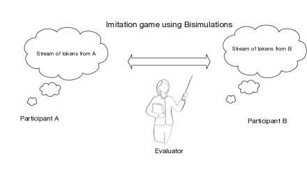
To begin with, we present an elegant formalism for solving static UIGs that is based on the concept of universal coalgebras Rutten (2000), and non-well-founded sets Aczel (1988). Figure 16 illustrates the main idea. We define the two participants in an imitation game as universal coalgebras (or non-well-founded sets) and ask if there is a bisimulation relationship between them. This characterization covers a wide range of probabilistic models, including Markov chains and Markov decision processes Sutton and Barto (1998), and automata-theoretic models, as well as generative AI models Gu et al. (2023).
Generative AI has become popular recently due to the successes of neural and structured-state space sequence models Gu et al. (2022); Vaswani et al. (2017) and text-to-image diffusion models Song and Ermon (2019). The underlying paradigm of building generative models has a long history in computer science and AI, and it is useful to begin with the simplest models that have been studied for several decades, such as deterministic finite state machines, Markov chains, and context-free grammars. We use category theory to build generative AI models and analyze them, which is one of the unique and novel aspects of this paper. To explain briefly, we represent a generative model in terms of universal coalgebras Rutten (2000) generated by an endofunctor acting on a category . Coalgebras provide an elegant way to model dynamical systems, and capture the notion of state Jacobs (2016) in ways that provide new insight into the design of AI and ML systems. Perhaps the simplest and in some ways, the most general, type of generative AI model that is representable as a coalgebra is the powerset functor
where is any set (finite or not), and is the set of all subsets of , that is:
Notice in the specification of the powerset functor coalgebra, the same term appears on both sides of the equation. That is a hallmark of coalgebras, and it is what distinguishes coalgebras from algebras. Coalgebras generate search spaces, whereas algebras compact search spaces and summarize them. This admittedly simple structure nonetheless is extremely versatile and enables modeling a remarkably rich and diverse set of generative AI models, including the ones listed in Figure 17. To explain briefly, we can model a context-free grammar as a mapping from a set that includes all the vertices in the context-free grammar graph shown in Figure 17 to the powerset of the set . More specifically, if is defined as the non-terminals as well as the terminal symbols (the actual words) , any context-free grammar rule can be represented in terms of a power set functor. We will explain how this approach can be refined later in this Section, and in much more detail in later sections of the paper. To motivate further why category theory provides an elegant way to model generative AI systems, we look at some actual examples of generative AI systems to see why they can be modeled as functors.
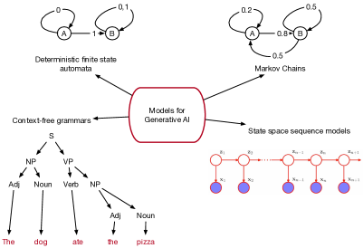
To solve Turing’s imitation game, we need to compare two potentially infinite data streams of tokens (e.g., words, or in general, other forms of communication represented digitally by bits). Many problems in AI and ML involve reasoning about circular phenomena. These include reasoning about common knowledge Barwise and Moss (1996); Fagin et al. (1995) such as social conventions, dealing with infinite data structures such as lists or trees in computer science, and causal inference in systems with feedback where part of the input comes from the output of the system. In all these situations, there is an intrinsic problem of having to deal with infinite sets that are recursive and violate a standard axiom called well-foundedness in set theory. First, we explain some of the motivations for including non-well-founded sets in AI and ML, and then proceed to define the standard ZFC axiomatization of set theory and how to modify it to allow circular sets. We build on the pioneering work of Peter Aczel on the anti-foundation-axiom in modeling non-well-founded sets Aczel (1988), which has elaborated previously in other books as well Barwise and Moss (1996); Jacobs (2016), although we believe this paper is perhaps one of the first to focus on the application of non-well-founded sets and universal coalgebras to problems in AI and ML at a broad level.
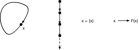
Figure 18 illustrates three ways to represent an infinite object, as a directed graph, a (non-well-founded) set or as a system of equations. We begin with perhaps the simplest approach introduced by Peter Aczel called accessible pointed graphs (APGs) (see Figure 18), but also include the category-theoretic approach of using universal coalgebras Rutten (2000), as well as systems of equations Barwise and Moss (1996).
We now turn to describing coalgebras, a much less familiar construct that will play a central role in the proposed ML framework of coinductive inference. Coalgebras capture hidden state, and enable modeling infinite data streams. Recall that in the previous Section, we explored non-well-founded sets, such as the set , which gives rise to a circularly defined object. As another example, consider the infinite data stream comprised of a sequence of objects, indexed by the natural numbers:
We can define this infinite data stream as a coalgebra, comprised of an accessor function head that returns the head of the list, and a destructor function that gives the tail of the list, as we will show in detail below.
To take another example, consider a deterministic finite state machine model defined as the tuple , where is the set of possible states that the machine might be in, is a set of input symbols that cause the machine to transition from one state to another, and specifies the transition function. To give a coalgebraic definition of a finite state machine, we note that we can define a functor that maps any given state to the subset of possible future states that the machine might transition to for any given input symbol .
We can now formally define -coalgebras analogous to the definition of -algebras given above.
Definition 64.
Let be an endofunctor on the category . An -coalgebra is defined as a pair comprised of an object and an arrow .
The fundamental difference between an algebra and a coalgebra is that the structure map is reversed! This might seem to be a minor distinction, but it makes a tremendous difference in the power of coalgebras to model state and capture dynamical systems. Let us use this definition to capture infinite data streams, as follows.
Here, Str is defined as a functor on the category Set, which generates a sequence of elements. Let denote the set of all infinite data streams comprised of natural numbers:
To define the accessor function head and destructor function tail alluded to above, we proceed as follows:
| (2) | |||||
| (3) |
Another standard example that is often used to illustrate coalgebras, and provides a foundation for many AI and ML applications, is that of a labelled transition system.
Definition 65.
A labelled transition system (LTS) is defined by a set of states, a transition relation , and a set of labels (or equivalently, “inputs" or “actions"). We can define the transition from state to under input by the transition diagram , which is equivalent to writing . The -coalgebra for an LTS is defined by the functor
Just as before, we can also define a category of -coalgebras over any category , where each object is a coalgebra, and the morphism between two coalgebras is defined as follows, where is any morphism in the category .
Definition 66.
Let be an endofunctor. A homomorphism of -coalgebras and is an arrow in the category such that the following diagram commutes:
For example, consider two labelled transition systems and over the same input set , which are defined by the coalgebras and , respectively. An -homomorphism is a function such that . Intuitively, the meaning of a homomorphism between two labeled transition systems means that:
-
•
For all , for any transition in the first system , there must be a corresponding transition in the second system in the second system.
-
•
Conversely, for all , for any transition in the second system, there exists two states such that such that in the first system.
If we have an -homomorphism with an inverse that is also a -homomorphism, then the two systems are isomorphic. If the mapping is injective, we have a monomorphism. Finally, if the mapping is a surjection, we have an epimorphism.
The analog of congruence in universal algebras is bisimulation in universal coalgebras. Intuitively, bisimulation allows us to construct a more “abstract" representation of a dynamical system that is still faithful to the original system. We will explore many applications of the concept of bisimulation to AI and ML systems in this paper. We introduce the concept in its general setting first, and then in the next section, we will delve into concrete examples of bisimulations.
Definition 67.
Let and be two systems specified as coalgebras acting on the same category . Formally, a -bisimulation for coalgebras defined on a set-valued functor is a relation of the Cartesian product of and is a mapping such that the projections of to and form valid -homomorphisms.
Here, and are projections of the relation onto and , respectively. Note the relationships in the two commutative diagrams should hold simultaneously, so that we get
Intuitively, these properties imply that we can “run" the joint system for one step, and then project onto the component systems, which gives us the same effect as if we first project the joint system onto each component system, and then run the component systems. More concretely, for two labeled transition systems that were considered above as an example of an -homomorphism, an -bisimulation between and means that there exists a relation that satisfies for all
-
•
For all , for any transition in the first system , there must be a corresponding transition in the second system in the second system, so that
-
•
Conversely, for all , for any transition in the second system, there exists two states such that such that in the first system, and .
A simple example of a bisimulation of two coalgebras is shown in Figure 19.
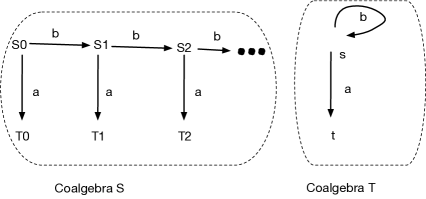
There are a number of basic properties about bisimulations, which we will not prove, but are useful to summarize here:
-
•
If is a bisimulation between systems and , the inverse of is a bisimulation between systems and .
-
•
Two homomorphisms and with a common domain define a span. The image of the span of and is also a bisimulation between and .
-
•
The composition of two bisimulations and is a bisimulation between and .
-
•
The union of a family of bisimulations between and is also a bisimulation.
-
•
The set of all bisimulations between systems and is a complete lattice, with least upper bounds and greatest lower bounds given by:
-
•
The kernel of a homomorphism is a bisimulation equivalence.
We can design a generic coinductive inference framework for systems by exploiting these properties of bisimulations. This framework will give us a broad paradigm for designing AI and ML systems that is analogous to inductive inference, which we will discuss in the next Section.
2.11 Static Imitation Games over Generalized Metric Spaces
A general principle in machine learning (see Figure 20) to discriminate two objects (e.g., probability distributions, images, text documents etc.) is to compare them in a suitable metric space. We now describe a category of generalized metric spaces, where a metric form of the Yoneda Lemma gives us surprising insight and yields a metric version of the Causal Reproducing Property stated above. Often, in category theory, we want to work in an enriched category Kelly (1982). One of the most interesting ways to design categories for applications in AI and ML is to look to augment the basic structure of a category with additional properties. For example, the collection of morphisms from an object to an object in a category often has additional structure, besides just being a set. Often, it satisfies additional properties, such as forming a space of some kind such as a vector space or a topological space. We can think of such categories as enriched categories that exploit some desirable properties. We will illustrate one such example of primary importance to applications in AI and ML that involve measuring the distance between two objects. A distance function is assumed to return some non-negative value between and , and we will view distances as defining enriched categories. We summarize some results here from Bonsangue et al. (1998).
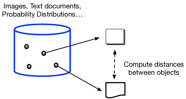
Figure 20 illustrates a common motif among many AI and ML algorithms: define a problem in terms of computing distances between a group of objects. Examples of objects include points in -dimensional Euclidean space, probability distributions, text documents represented as strings of tokens, and images represented as matrices. More abstractly, a generalized metric space is a set of objects, and a non-negative function that satisfies the following properties:
-
1.
: distance between the same object and itself is .
-
2.
: the famous triangle inequality posits that the distance between two objects cannot exceed the sum of distances between each of them and some other intermediate third object.
In particular, generalized metric spaces are not required to be symmetric, or satisfy the property that if the distance between two objects and is implies must be identical to , or finally that distances must be finite. These additional three properties listed below are what defines the usual notion of a metric space:
-
1.
If and then .
-
2.
.
-
3.
.
In fact, we can subsume the previous discussion of causal inference under the notion of generalized metric spaces by defining a category around preorders , which are relations that are reflexive and transitive, but not symmetric. Causal inference fundamentally involves constructing a preorder over the set of variables in a domain. Here are some examples of generalized metric spaces:
-
1.
Any preorder such that all , if and , then, , and , where
-
2.
The set of strings over some alphabet defined as the set where the distance between two strings and is defined as
-
3.
The set of non-negative distances where the distance between two objects and is defined as
-
4.
The powerset of all subsets of a standard metric space, where the distance between two subsets is defined as
which is often referred to as the non-symmetric Hausdorff distance.
Generalized metric spaces can be shown to be -enriched categories as the collection of all morphisms between any two objects itself defines a category. In particular, the category is a complete and co-complete symmetric monoidal category. It is a category because objects are the non-negative real numbers, including , and for two objects and in , there is an arrow from to if and only if . It is complete and co-complete because all equalizers and co-equalizers exist as there is at most one arrow between any two objects. The categorical product of two objects and is simply , and the categorical coproduct is simply . More generally, products are defined by supremums, and coproducts are defined by infimums. Finally, the monoidal structure is induced by defining the tensoring of two objects through “addition":
where is simply their sum, and where as usual .
The category is also a compact closed category, which turns out to be a fundamentally important property, and can be simply explained in this case as follows. We can define an “internal hom functor" between any two objects and in the distance as defined above, and the co pre-sheaf is right adjoint to for any .
Theorem 15.
For all and ,
We will explain the significance of compact closed categories for reasoning about AI and ML systems in more detail later, but in particular, we note that reasoning about feedback requires using compact closed categories to represent “dual" objects that are diagrammatically represented by arrows that run in the “reverse" direction from right to left (in addition to the usual convention of information flowing from left to right from inputs to outputs in any process model).
We can also define a category of generalized metric spaces, where each generalized metric space itself as an object, and for the morphism between generalized metric spaces and , we can choose a non-expansive function which has the contraction property, namely
where is assumed to be some real number that lies in the unit interval. The category of generalized metric spaces will turn out to be of crucial importance in this paper as we will use a central result in category theory – the Yoneda Lemma – to give a new interpretation to distances.
Finally, let us state a “metric" version of the Yoneda Lemma specifically for the case of -enriched categories in generalized metric spaces:
Theorem 16.
Bonsangue et al. (1998) (Yoneda Lemma for generalized metric spaces): Let be a generalized metric space. For any , let
Intuitively, what the generalized metric version of the Yoneda Lemma is stating is that it is possible to represent an element of a generalized metric space by its co-presheaf, exactly analogous to what we will see below in the next section for causal inference! If we use the notation
to indicate the set of all non-expansive functions from to , then the Yoneda embedding defined by is in fact a non-expansive function, and itself an element of ! Thus, it follows from the general Yoneda Lemma that for any other element in ,
Another fundamental result is that the Yoneda embedding for generalized metric spaces is an isometry. Again, this is exactly analogous to what we see below for causal inference, which we will denote as the causal reproducing property.
Theorem 17.
The Yoneda embedding , defined for by is isometric, that is, for all , we have:
Once again, we will see a remarkable resemblance of this result to the Causal Representer Theorem below. With the metric Yoneda Lemma in hand, we can now define a framework for solving static UIGs in generalized metric spaces.
Definition 68.
Two objects and are isomorphic in a generalized metric space category if they are isometrically mapped into the category by the Yoneda embedding and such that , where they can be defined isomorphically by a suitable pair of suitable natural transformations.
Imitation Games using Coalgebraic Behavioral Distances
We can build on the theory of generalized metric spaces to define behavioral distance metrics on coalgebras Baldan et al. (2014). These distance metrics can be then used to define a way to formulate UIGs based on comparing two participants based on a coalgebraic model of them. The basic idea of behavioral distance metrics is lifting of functors. A coalgebra defined by a functor on the category of Sets is lifted to the category of (generalized or pseudo) metric spaces. Then, behavioral distances can be defined with respect to the lifted functor . These can be shown to correspond to well-known distance metrics in optimal transport Villani (2003), such as Wasserstein distances or Kantorovich distances.
Imitation Games in Generalized Metric spaces over the Category of Wedges
Note we can also generalize previous work on behavioral metrics for coalgebras by extending them to generalized metric spaces using the metric Yoneda embedding Bonsangue et al. (1998). We can also define imitation games over the category of wedges defined as a collection of objects , and the arrows are defined as dinatural transformations. We leave these extensions to a future paper.
3 Dynamic Universal Imitation Games: From Inductive to Coinductive Inference
In the case when the participants are changing during the course of the interactions, we need to consider how a participant changes over the course of interactions. In dynamic UIGs, “learner" participants imitate “teacher" participants. We show here that initial objects correspond to the framework of passive learning from observation over well-founded sets using inductive inference – expensively studied by Gold Gold (1967) Solomonoff Solomonoff (1964) Valiant Valiant (1984) and Vapnik Vapnik (1999). In contrast, final objects correspond coinductive inference over non-well-founded sets and universal coalgebras Jacobs (2016); Rutten (2000), which includes learning from active experimentation corresponding to causal inference Imbens and Rubin (2015) or reinforcement learning Sutton and Barto (1998). We define a category-theoretic notion of minimum description length or Occam’s razor based on final objects in coalgebras.
We now introduce coinductive inference, a novel theoretical foundation for ML that is based on the conceptualization of non-well-founded sets in terms of APGs Aczel (1988), graphs not sets, or in terms of universal coalgebras Rutten (2000). Put succinctly, the difference between coinductive inference vs. inductive inference lies in that in the former, APGs (or equivalently universal coalgebras) are enumerated to find one consistent with the teacher’s presentation. In contrast, as we saw above, inductive inference is based on enumerating recursively enumerable sets, which do not allow for non-well-founded sets.
The term coinductive inference, which we introduce in this paper, is based on coinduction, a proof principle, developed initially by Peter Aczel in his ground-breaking work on non-well-founded circular (or recursively defined) sets Aczel (1988). Figure 21 illustrates the general framework of coinductive inference that is based on the theory of universal coalgebras. Comparing the framework for inductive inference presented above, the major difference is the use of AGPs or universal coalgebras as the formalism for describing the language used by the teacher to specify a particular model from which data is generated, and by the learner to produce a solution. Universal coalgebras provide a universal language for AI and ML in being able to describe a wide class of problems, ranging from causal inference, (non)deterministic and probabilistic finite state machines, game theory and reinforcement learning.
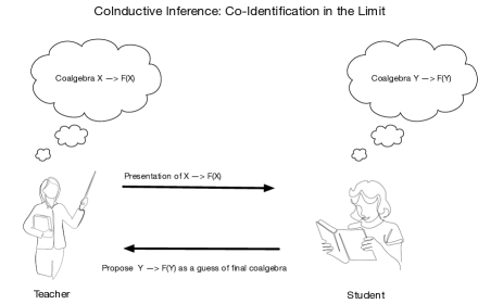
To take some concrete examples, let us begin with the standard problem of learning a deterministic finite state machine model. We can specify a finite state machine model as a labeled transition system consisting of a set of states, a transition relation , where is a set of input labels. Let us define a functor for any set . is then an endofunctor on the category of sets, which specifies the transition dynamics of the finite state machine. We can then represent a labelled transition system as a universal coalgebra of the following type:
for some fixed set of input symbols . The coinductive inference framework assumes the teacher selects a particular coalgebra specifying a finite state machine and generates a presentation of it for the learner. Upon receiving a sequence of examples, the learner produces a hypothesis coalgebra describing the finite state machine. The learner’s ultimate goal can be succinctly summarized as discovering the final coalgebra that represents the minimal finite state machine model that is isomorphic to the coalgebra selected by the teacher.
In this second class of UIGs, we turn from Turing’s original question “Can machines think?" to “Can machines learn?". We , we turn to discuss the fundamental question “Can machines learn?". As with the previous case, we have to define what “learn" means. We introduce a categorical perspective that neatly spans the initial object framework of inductive inference over well-founded sets proposed by Gold Gold (1967) and Solomonoff Solomonoff (1964) and later refined by Valiant Valiant (1984) and Vapnik Vapnik (1999) to the probabilistic case, with the final object coinductive inference, a categorical framework over non-well-founded sets based on universal coalgebras Jacobs (2016); Rutten (2000) framework for ML based on coidentification in the limit. Inductive inference is formulated in the traditional realm of ZFC set theory, which does not permit non-well-founded sets. Aczel Aczel (1988) introduced a formalism for non-well-founded sets using graphs, and developed a coinduction principle for reasoning about circular sets. This framework was later extended by Rutten for the study of dynamical systems. We show a wide range of generative AI and ML systems can be modeled as endofunctors that act on specific categories. Algebras compress and summarize information. Coalgebras, in contrast act as generators and enable rigorously modeling non-well-founded infinite data streams produced by generative models, including automata, grammars, probabilistic transition models among others. Coidentification in the limit is defined as finding a final coalgebra in a category of coalgebras. Final coalgebras generalizes the use of (greatest) fixed points. We introduce the theory of monads, which gives an elegant framework to integrate algebraic and coalgebraic reasoning, and provides a categorical foundation for modeling probabilities, Markov chains and stochastic processes.
Before introducing our novel formulation of ML as coinductive inference over non-well-founded sets, we want to give a brief historical review of ML, focusing on the theoretical framework of inductive inference that has been the cornerstone of the field for many decades, originally introduced by Gold Gold (1967), Solomonoff Solomonoff (1964) and others based on the principle of mathematical induction over well-founded sets. Induction is a natural way to model learning as a process of generalizing rules from examples. A long tradition in philosophy, dating back to Hume Hume (1740) and even before to Aristotle Aristotle (1984) have thought about learning as induction. We first briefly review the framework of Gold on inductive inference or identification in the limit, and then describe probably approximately correct (PAC) learning introduced by Valant Valiant (1984) that addressed some limitations of the Gold paradigm. We finally discuss some limitations of the PAC model as well.
Humans appear singularly adept at inducing general rules from even a relatively small number of well-chosen examples, an ability that provides the foundation for many of our intellectual capabilities, from learning language to motor behavior and social skills. Figure 22 illustrates a problem of visual induction introduced by Bongard Bongard (1970) in his book on pattern recognition. Bongard’s book featured a collection of several hundred such problems of varying difficulty, which can be found online as well. 333See https://www.foundalis.com/res/bps/bpidx.htm for a listing of Bongard problems.
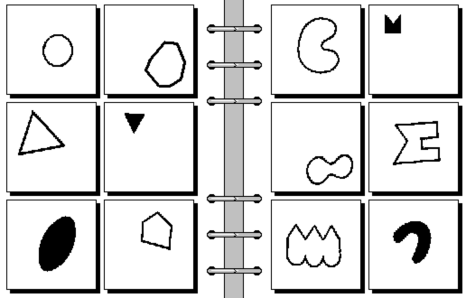
Our ability at inducing patterns from examples extends across modalities. Consider, for example, the problem of inducing a function over the natural numbers, from a sequence of examples such as the one below:
1, 2, 3, 5, 7, 11, 13, ...
This sequence immediately brings our attention to the possibility that the sequence in question represents the prime numbers, numbers that are not divisible by any other number except and themselves. We can immediately see that the problem of induction seems ill-posed, as there may be many hypotheses consistent with a given sequence of examples, and it may not be possible to determine the right hypothesis from the given data. For example, consider the inductive inference problem posed by the initial part of the above sequence:
1, 2, 3, ...
In this case, the number of possible hypotheses could be enormous. Certainly, it would include the previous hypothesis about the sequence being the prime numbers, but it could also be all natural numbers, or many other possibilities. It is relatively easy to design inductive inference problems that can defeat any learner based on some initial presentation. Consider the following somewhat contrived example:
0, 0, 0, 0, ...
In this case, the learner might conjecture that this sequence is simply the set of all ’s, but it could have been generated from the following polynomial:
in which case the correct answer for the fifth element in the sequence is:
0, 0, 0, 0, 24, ...
Finally, let us consider an adversarial setting, where a teacher simply generates a sequence that keeps changing depending on a learner’s guesses. Such considerations suggest that to define a useful model of ML using inductive inference, additional structure must be imposed to make the problem well-defined. We now review the most influential models of ML next, beginning with the model of inductive inference: identification in the limit.
3.1 Passive Learning: Inductive Inference over Well-Founded Sets
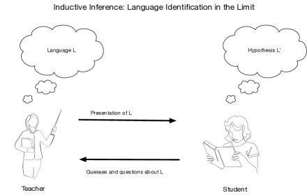
We briefly describe a formal theory of inductive inference proposed by Solomonoff in 1964, and further studied by Gold in a classic paper in 1967. Figure 23 describes the setting of language identification in the limit, a model of inductive inference proposed by Gold in 1967. In this framework, a teacher selects a candidate language from some hypothesis space of possible languages, and constructs a presentation of to teacher a student learner. The student’s task is to identify the unknown language from the teacher’s presentation. The term identification in the limit is intended to reflect the continuing nature of this inductive inference task. This original setting of inductive inference is intended similar to the theoretical model of computability: are there intrinsic limitations to induction as a model of ML, independent of computational complexity criteria or any finiteness considerations? Table 4 summarizes Gold’s principal results. To understand the table, we need to define the main components of this model more carefully, as this structure will also inform the design of our coinductive inference framework later in this paper.
| Model | Languages | Learnable? |
| Anomalous text | Recursively enumerable | Yes |
| Recursive | Yes | |
| Informant | Primitive Recursive | Yes (not above) |
| Context-sensitive | Yes | |
| Context-free | Yes | |
| Regular | Yes | |
| Super-finite | Yes | |
| Text | Finite | Yes (not above) |
A language learnability model, as defined by Gold, consisted of the following components:
-
1.
A definition of learnability: Gold focused on identifiability in the limit.
-
2.
A method of information presentation: Table 4 includes anomalous text, informant, and text.
-
3.
A naming relation: Gold focused on principally two naming relations, including a tester, and a generator.
This conceptualization is fundamentally set-theoretic: identification in the limit implies naming a well-founded set through some method, such as enumeration of all recursively enumerable sets. In practice, more efficient methods have been developed over the past 60 years, and we focus on one particularly instructive framework next.
Inductive Inference using Version Spaces
As a concrete example of an inductive inference algorithm, in this section we describe Tom Mitchell’s version spaces framework Mitchell (1977) (see Figure 24). Version spaces is particularly interesting as it specifies not one specific algorithm, but rather a broad framework that can be specialized in many ways to design more specific methods. The set represents the set of all maximally specific hypotheses consistent with the data, whereas the set represents the set of all maximally general hypotheses consistent with the data. The notion of specificity or generality is with respect to the partial ordering implicit in the lattice structure shown in Figure 23. Bringing in the category-theoretic perspective, the lattice structure can be defined as a preorder category , where is the set of all hypotheses under consideration (e.g., all context-free languages), and is a reflexive transitive relationship on hypotheses. A morphism exists between hypotheses and when . As we will show later, computing the maximally specific and maximally general hypotheses in a version space corresponds to computing the meets and joins in a partial order, respectively, or more generally, finding the limits and colimits of universal diagrams .
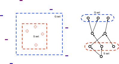
Probably Approximately Correct Learning
A significant weakness of the original inductive inference model proposed by Gold is that it required the learner to exactly identify a language, and it did not impose any computational requirement in terms of the number of examples required or the amount of time needed for identification. In an influential paper published in the Communications of the ACM, Valiant proposed a significantly revised model of inductive inference in 1984 that has come to be known as probably approximately correct (PAC) learning Valiant (1984). In PAC learning, the data is assumed to be generated by some unknown (to the learner) but fixed probability distribution over a hypothesis space (e.g., strings generated by a regular language associated with a finite state automata). The goal for the learner is to discover an approximation of the unknown function that is accurate as measured by its differences with the true function on data that is sampled from the distribution . In this setting, accuracy is defined as the probability that a randomly chosen point will result in the outcome . The goal is to find an approximate hypothesis such that the probability of disagreement can be bounded by some scalar value :
However, since the teacher uses the distribution to sample instances, an unlucky run of truly “bad" examples cannot be ruled out, but the goal is to ensure that such an unrepresentative set of training examples occurs rarely. In other words, the learner is allowed to fail, but with probability bounded by a second parameter . The aim of PAC learning is to determine for any given class of hypotheses whether every function can be identified in the PAC sense using only polynomially many examples in the parameters (size of a hypothesis), and . The intuition here is that and are reduced closer to , requiring the learner to produce a more accurate hypothesis more reliably, the number of examples will grow as well. Valiant’s PAC framework was further generalized by combining it with the notion of dimensionality proposed by Vapnik and Chervonenkis, which came to be known as the VC-dimension Vapnik (1999). A fundamental result in this setting was that a hypothesis class is polynomially sample PAC learnable if its VC-dimension was finite (in the continuous setting) or polynomial in the relevant parameters (, , ). In the particular case where the hypothesis space is all axis-parallel rectangles on , the VC-dimension is as no training set of size larger than can be “shattered". A training data set can be shattered if there exists a hypothesis that is consistent with every possible labeling of the points in . In the case of axis-parallel rectangles, there exists a set of points on the plane where the interior point can be labeled and the remaining points labeled , and no hypothesis in is consistent with this labeling. In more concrete terms, using the example hypothesis space of all axis-parallel rectangles in Figure 24, it suffices to maintain one hypothesis rectangle consistent with all the training data seen so far, and it can be shown that the version space of all consistent hypotheses (i.e., axis-parallel rectangles) can be -exhausted given polynomially many samples in the VC-dimension (which is in this case) and accuracy parameter and reliability parameter Haussler (1988, 1987).
High-Dimensional Statistics: Limitations of the PAC Model
In practice, there are a number of significant limitations of the PAC model, mostly having to do with its inability to exploit the actual structure that exists in many real-world machine learning problems (see Figure 25). In high-dimensional statistics, data tends to exhibit a concentration effect. In low dimensions, a uniform distribution of data points in a a hypersphere appear scattered throughout, but as the dimensionality increases, much of the data concentrates on the boundary. The set of all covariance matrices that might summarize statistical properties of datasets that lie in vector spaces forms a nonlinear manifold. It is possible to exploit such statistical and topological regularities to design efficient inductive inference algorithms that behave far better in high-dimensional problems that the idealized PAC bounds would predict. In addition, there seems to be a growing realization that the phenomenon of overfitting, where a model has a very large number of parameters, such as the billions of weights in large language models Vaswani et al. (2017), is not as problematic as some of the simplified statistical models would predict Poggio et al. (2018).
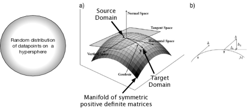
Algorithmic Information Theory and Kolmogorov Complexity
The mathematician Kolmogorov proposed in 1965 a model of the intrinsic complexity of an object, which can be viewed as a rigorous definition of inductive inference based on the heuristic of Occam’s razor: the simplest explanation is the best. Kolmogorov complexity can be viewed as an intellectual predecessor to information theory, as it does not depend on a probability distribution, and has been proposed as a universal probability model Vitányi (2013). Chaitin proposed a similar framework called algorithmic information theory Chaitin (2002).
As we discuss below, we use coinductive inference to propose a new perspective on characterizing minimum description length type formulations in terms of the final coalgebras. As we will see later, in categories of coalgebras generated by a functor that admits a final coalgebra, a representation is minimal if the unique morphism mapping it to the final coalgebra is injective. This category-theoretic reformulation of the MDL principle is one of the novel aspects of our formulation of ML, which we turn to describe in more detail now.
Categorical Version Spaces using Ends and Coends
We can generalize the classic version space algorithm Mitchell (1977) to arbitrary categories, by modeling the process of finding the and sets in terms of the limits and colimits of a set of data points. We can use the simplicial set representation introduced in the previous section, and used in dimensionality reduction methods such as UMAP McInnes et al. (2018). We leave this extension to a future paper.
3.2 Passive vs. Active Learning in Dynamic UIGs: Statistical vs. Causal Inference
To make the transition from inductive inference over well-founded sets to coinductive inference over non-well-founded sets and universal coalgebras, we work through a series of more concrete examples, starting with the distinction between passive statistical learning from data Belkin et al. (2006) vs. learning from active experimentation. We use as examples the difference between building a statistical model based on conditional independences, vs. doing causal inference, as well as learning a finite state machine model from passive observation vs. learning a diversity automata from experimentation Rivest and Schapire (1994).
To define UIGs over statistical models, we define a category of objects, where each object abstractly represents a statistical model in terms of a set of conditional independences Dawid (2001); Pearl (2009). Conditional independence is a foundational concept in statistics, which finds many applications to problems in AI and ML, including structured representations of probabilistic graphical models, causal inference, and estimation of statistical models from data. One can define a generalized algebraic notion of conditional independence in terms of separoids.
A separoid is defined as a semi-lattice , where the join operator over the semi-lattice defines a preorder , and the ternary relation is defined over triples of the form (which are interpreted to mean is conditionally independent of given ). We show briefly how to define a category for universal conditional independence, where each object is a separoid, and the morphisms are homomorphisms from one separoid to another. It is possible to define “lattice” objects in any category by interpreting an arrow as defining the partial ordering.
Definition 69.
A separoid defines a category over a preordered set , namely is reflexive and transitive, equipped with a ternary relation on triples , where satisfy the following properties:
-
•
S1: is a join semi-lattice.
-
•
P1:
-
•
P2:
-
•
P3:
-
•
P4:
-
•
P5:
A strong separoid also defines a categoroid. A strong separoid is defined over a lattice has in addition to a join , a meet operation, and satisfies an additional axiom:
-
•
P6: If and , then
To define a category of separoids, we have to define the notion of a homomorphism between separoids:
Definition 70.
Let and be two separoids. A map is a separoid homomorphism if:
-
1.
It is a join-lattice homomorphism, namely , which implies that .
-
2.
.
-
3.
In case both S and S’ are strong separoids, we can define the notion of a strong separoid homomorphism to additionally include the condition: .
With this definition, we can now define the category of separoids and a representation-independent characterization of universal conditional independence as follows:
Theorem 18.
The category of separoids is defined as one where each object in the category is defined as a separoid , and the arrows are defined as (strong) separoid homomorphisms. The category of separoids provides an axiomatization of universal conditional independence, namely that it enables a universal representation through the use of universal arrows and Yoneda lemma.
Proof.
First, we note that the category of separoids indeed forms a category as it straightforwardly satisfies all the basic properties. The (strong) separoid homomorphisms compose, so that as a composition of two (strong) separoid homomorphisms produces another (strong) separoid homomorphism. The universal property derives from the use of the Yoneda lemma to define a category of presheaves that map from the category of separoids to the category Sets. ∎
With this category of separoids defined, we can formulate a static UIG over separoids as follows:
Definition 71.
Two objects and in a category of separoids are isomorphic if there is a separoid homomorphism and a separoid homomorphism such that and .
Causal Imitation Games
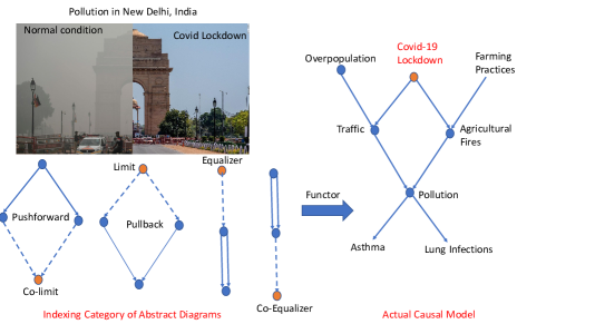
Causal imitation games have been extensively studied (see Table 5) for over a hundred years, ever since Darwin asked Galton to help him design a test that would separate out two species of plants that he had grown under different conditions Darwin (1876). Galton proposed a rank-ordered statistic, where the plants are all ranked by height, and the imitation game can be solved (i.e., variant of type 1 can be discriminated from variant of type 2) if the specific ordering can be shown to be different from what one would expect in a random ordering. Since that time, for 150 years, researchers in every area of science have developed techniques for deciding if two groups of objects are the same or different, under the condition where one group can be subjected to some experiment. A thorough review of these techniques under the framework of potential outcomes is given in Imbens and Rubin (2015). The name derives from the fact that causal inference invariably involves counterfactuals due to unobservable confounders: the test group of objects is administered a treatment, whereas the control group is not, and the data from the experiment does not reveal the counterfactual outcomes. In computer science, causal inference has been studied on directed acyclic graphs (DAGs) Pearl (2009), and more recently, on categories Fong (2012); Fritz and Klingler (2023); Mahadevan (2023). We review some of the main concepts here, with a special emphasis on our recent framework of universal causality Mahadevan (2023).
Humans have sought to understand causality since ancient times. 2500 years ago, Plato remarked that "Everything that becomes or changes must do so owing to some cause; for nothing can come to be without a cause". Even a cursory study of the past literature on causal inference would immediately overwhelm the reader, since a veritable “Tower of Babel" repertoire of languages and representations have been proposed to understand causality (see Table 5). Category theory can be viewed as a “Rosetta Stone" Baez and Stay (2010) to translate across diverse representations used in causal inference. In a recent paper Mahadevan (2023), we showed that the Yoneda Lemma provides deep insight into the nature of causal reasoning, through both theoretical results as well as providing an elegant way to capture universal properties of causality. Specifically, we identified the Causal Reproducing Property, a special case of the Yoneda Lemma, that shows that the contravariant functor is the principal carrier of causal information in a category (which by default includes all the work on categorical modeling over directed graphs Pearl (2009)).
| Representation | Objects | Morphisms | References |
|---|---|---|---|
| Graphs | Variables | Paths | Pearl (2009) |
| Topological Spaces | Open sets | Fences | Bradley et al. (2022b) |
| Information fields | Measurable Spaces | Measurable mappings | Mahadevan (2021b) |
| Resource Models | Monoidal resources | Profunctors | Fong and Spivak (2018) |
| Concurrent Systems | Program variables | Bisimulation morphisms | Joyal et al. (1996) |
| Dynamical systems | States | Processes | Mahadevan (2021b) |
| Counterfactuals | Propositions | Proofs | Lewis (1973) |
| Network Economy | Consumers/Producers | Trade | Nagurney (1999) |
| Discourse Sheaves | Users | Communication | Hansen and Ghrist (2020) |
As a concrete example, Judea Pearl developed an approach to causal inference based on directed acyclic graph (DAG) models, where a variable can exert a causal influence on variable if a directed path exists between and . Pearl’s framework suggests an immediate categorical treatment, as the paths in a directed graph in fact correspond directly to the morphisms in the so-called free category associated with the graph. We can define causal models in terms of functors that act on a category of algebraic structures, mapping them to a category of probabilistic representations defined as morphisms over a Kleisli category of a Giry monad Giry (1982). In effect, a Bayesian network causal model is in fact a functor, because it is more than a graph, it is a mapping of a graph onto a structured probability distribution. A Bayesian network is more appropriately thought of as a functor that maps between two categories, a syntactic category of graphs as algebraic structures and a semantic category of probability distributions. Thinking of Bayesian networks as functors opens the door to including more sophisticated ideas. We can introduce universal constructions from category theory, including the limit or co-limit of an abstract causal diagram, or more generally, the Kan extension. We can formalize Plato’s insight using the Yoneda Lemma, since every variable in a causal model is influenced by the set of all variables that can act on it through some causal pathway. This notion can be made formal through the Yoneda Lemma by constructing the presheaf contravariant functor from the category defining a causal model into a category of probability distributions or sets.
Figure 26 illustrates the main idea of using category theory to formalize causal inference using a real-world example showing how a natural intervention experiment caused by the Covid pandemic caused a significant reduction in the air quality in New Delhi, India, one of the world’s most polluted cities. Causality studies the question of how an object (e.g., air pollution in New Delhi, India) changes due to an intervention on another object (e.g., Covid-19 lockdown). Causal influences are transmitted along paths in a causal model. In the directed acyclic graph (DAG) model shown, causal influence corresponds to a directed path from a variable into another variable Pearl (2009). Covid-19 lockdown caused both a reduction in traffic as well as less burning of crops, both of which dramatically reduced air pollution in New Delhi. Universal Causality (UC) formulates the problem of causal inference in an abstract category of causal diagrams, of which DAGs are one example, where objects can represent arbitrary entities that interact in diverse ways (see the range of possibilities in Table 5).
One fundamental theoretical insight provided by category theory is the universality of diagrams in causal inference. More formally, any causal inference can be defined as an object in the contravariant functor category Set of presheaves, which is representable as the co-limit of a small indexing diagram that serves as its universal element. The notion of a diagram is more abstract than previous diagrammatic representations in causal inference (see Figure 27). For example, in causal inference using DAGs, a collider node defines the structure . In our framework, an abstract causal diagram functorially maps from an indexing category of diagrams, such as into the actual causal diagram . Abstract causal diagrams themselves form a category of functors. The fundamental notion of a limit or co-limit of a causal diagram are abstract versions of more specialized universal constructions, such as “pullbacks", “pushouts", “co-equalizers" and “equalizers", commonly used in category theory, but hitherto not been studied in causal inference. For example, the limit of the abstract causal diagram mapping into the actual causal model is defined as a variable, say , that acts as a “common" cause between and in a “universal" manner, in that any other common cause of and must factor through . In fact, a rich repertoire of other construction tools have been developed in category theory, including Galois extensions, adjunctions, decorated cospans, operads, and props, all of which enable building richer causal representations than have been previously explored in the causal inference literature.
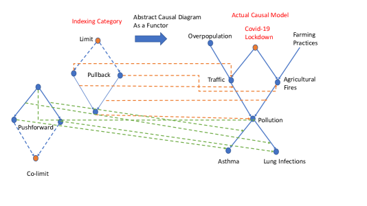
We want to briefly discuss a central result that we call the Causal Reproducing Property, as it is analogous to a key result in machine learning in the literature on kernel methods. Reproducing Kernel Hilbert Spaces (RKHS’s) transformed the study of machine learning, precisely because they are the unique subcategory in the category of all Hilbert spaces that have representers of evaluation defined by a kernel matrix Schölkopf and Smola (2002). The reproducing property in an RKHS is defined as . An analogous but far more general reproducing property holds in the categorical causality framework, based on the Yoneda Lemma.
Theorem 19.
Mahadevan (2023) The causal reproducing property (CRP) states that the set of all causal influences between any two objects and can be defined from its presheaf functor objects, namely Hom Nat(Hom,Hom.
Proof: The proof of this theorem is a direct consequence of the Yoneda Lemma, which states that for every presheaf functor object in of a category , Nat(Hom. That is, elements of the set are in bijections with natural transformations from the presheaf Hom to . For the special case where the functor object Hom, we get the result immediately that Hom Nat(Hom,Hom.
The significance of the Causal Reproducing Property is that presheaves act as “representers" of causal information, precisely analogous to how kernel matrices act as representers in an RKHS. Remarkably, we show below that an analogous result holds in a completely different setting, that of generalized metric spaces that is again of central importance in machine learning. Thus, the framework for causal imitation games can be defined in terms of the causal reproducing property.
Definition 72.
Two objects and in a category of causal models are isomorphic if there is a natural transformation and a natural transformation such that defines a natural isomorphism between the presheaves of and that act as representers of causal information.
3.3 Dynamic UIGs using Experimentation: Learning Diversity Automata
In this section, we give another example of solving dynamic UIGs using active experimentation, which illustrates an interesting diversity representation of automata to model environments that are often studied in AI, including games such as Rubik’s cube. The goal is to understand how a robot can construct a model of an unknown environment whose states it cannot completely observe by conducting experiments with it. This approach of using tests to reveal the underlying state of an environment relates to work in coalgebras on using traces to define the underlying semantics, which provides an interesting example to explain the coalgebraic approach. We call this diversity coalgebras to reflect the marriage of two viewpoints.
This approach of using diversity representations for modeling finite state automata was originally proposed in the category theory literature by Arbib, Bainbridge and others, but popularized in the ML literature by Rivest and Schapire. The use of diversity representations provides an interesting example of universal coalgebras. Rivest and Schapire specify environments as (Moore) finite state automata is defined by them as a finite nonempty set of states, a finite nonempty set of input symbols or “actions" , a finite nonempty set of predicate symbols or “sensations" , an initial state , a state transition function , and finally an output function . What is interesting about the diversity representation is that it represents an alternate way to specify environments, not in terms of specifying states (which might be unobservable), but in terms of a collection of tests. The standard notion of accepting states in a finite state machine can be viewed as a special case of a single accept predicate. Rivest and Schapire show a diversity representation can be constructed using an update graph whose vertices are tests, defined as sequences of input symbols followed by one or more predicate symbols that determine if a particular test succeeds in that state. We explore the problem of constructing the diversity automata from experiments in a later Section. Right now, we want to focus on defining a diversity coalgebra to show how to design more compact representations of finite state machines than the usual state-based framework.
Let us define by the set of all strings of input symbols, and extend the transition function suitably as . A test is defined as an element of the concatenated set , namely an action followed by a predicate . The set of all possible tests is denoted by . A test succeeds in a state if . Otherwise, we declare the test as failed. An environment is reduced if every pair of states can be distinguished by executing some test:
The goal is to be able to predict the results of doing any test, by which a robot can be assumed to have a perfect model of its environment even if it is unable to perceive the true underlying state of the environment. We will see interesting examples of environments, such as the Rubik’s cube, where the diversity representation is far more compact than the traditional state-based approach. A key notion is the use of equivalences among tests. Two tests and are considered equivalent, or if
This equivalence relation partitions the state space into equivalence classes, so we can denote the equivalence class of a test by . The diversity of an environment, defined as is defined as the number of equivalence classes of tests.
A simple result to prove is that the diversity can be exponentially smaller than the number of states, but it can also be substantially larger. Thus, whether the diversity approach is beneficial depends entirely on a specific environment. It turns out that a large number of natural environments seem to be highly compact in terms of their diversity. Figure 28 illustrates a simple -bit register world environment, where the state space grows exponentially in , but the diversity representation can be exponentially smaller.
Theorem 20.
For any reduced finite-state automaton , the diversity measure is in the following range:
The proof is straightforward: a state is uniquely identified by the set of equivalence classes of tests that are true at that state, as we assume the automaton is reduced, and hence any two states can be distinguished by some test. The lower bound simply states that the number of states . The upper bound holds because the equivalence class that a test defines is defined by the set of possible states where that equivalence class succeeds.
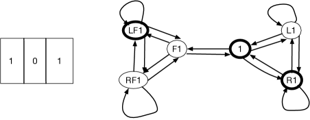
As shown in Figure 29, we can define two categories of representations of environments, one based on a traditional state-based finite automata and the other based on the Rivest and Schapire diversity representation. We can define an adjoint functor that maps between the two categories, where the left adjoint maps a given state based environment (such as the one illustrated in Figure 28) into its equivalent diversity-based representation, and the right adjoint maps a diversity-based automata into its state-based representation. Note that these functors must act functorially, which means that they map not only objects (i.e., state-based or diversity-based environment automata), but also the corresponding morphisms. To define these functors more formally, let us make more precise the two categories.

Definition 73.
The category CS of state-based environments is defined by as a collection of objects, where each object is a state-based automata as defined previously. Given a pair of environments in , each morphism in is defined by a set of functions that maps each state of into the corresponding state of , maps each input action symbol of into the corresponding action symbol of , maps each predicate symbol of into the corresponding symbol of , that maps the transition function of into the corresponding transition function of such that , and finally maps the output function of into the corresponding output function of such that .
We will define below more precisely the notion of bisimulation that specifies when a state-based environment can faithfully simulate another state-based environment (and equivalently when one diversity-based environment can be simulated by another environment ). Here, we want to briefly describe how the adjoint functors can be implemented as well, so that a diversity-based environment can simulate a state-based environment. Note from the example of the -bit register in Figure 28, the functor mapping a state-based environment to a diversity based environment might be “lossy" depending on whether an adequate set of tests are used. For example, if all the diversity-based environment cares about is whether the leftmost bit is a or , it might be sufficient to use tests that are adequate to predict that, but not sufficient to predict the entire state-based automaton’s transitions. However, given sufficient number of tests, which as was shown above might be exponentially larger (or smaller) than the number of states, the adjoint functors can be made faithful in both directions. Given a state-based representation of an environment , the following result is easy to show.
Theorem 21.
To simulate a state-based environment , which means to be able to predict the results of running every test in , it is sufficient to build a diversity-based environment , and for each equivalence class of tests represented as a vertex in the diversity-based environment , the value at the current state of .
To prove this, note that if the state-based automaton moves from state to the state for some input , the diversity-based automaton needs to compute for each equivalence class of tests . The test belongs to the unique equivalence class for which an edge labeled is directed from to in the diversity-based automata representation. We can use this insight to define the category of diversity-based environments.
Definition 74.
The category CD of diversity-based environments is defined by as a collection of objects, where each object is a diversity-based automata , where is a set of tests comprised of an action sequence followed by a predicate symbol , is a set of input “action" symbols, is the test transition function, and maps each equivalence class of tests into its value or in the current state. Given a pair of environments in , each morphism in is defined by a set of functions that maps each test of into the corresponding test of , maps each input action symbol of into the corresponding action symbol of , maps the test transition function of into the corresponding test transition function such that , and finally maps the output function for into that for such that
Finally, we can define the category of coalgebras for diversity-based environments using the above definitions.
Definition 75.
The category of coalgebras of diversity-based environments is defined as a collection of objects, where each object is defined as a coalgebra where is a diversity-based environment, is an endofunctor on diversity-based environments defined by that simulates a state-based environment on any input symbol, and each morphism in is defined as such that the following diagram commutes for any morphism over diversity-based environments that maps the environment into :
We want to introduce a topological perspective here, which will become important in later Sections. Essentially, modeling an environment in terms of its diversity is tantamount to defining a topology on the state space of a finite-state machine, where each (open) set represents the set of states where a particular equivalence class of tests succeeds. An automaton is reduced if it defines a Hausdorff topology, that is, for any pair of elements and , there is an open set that contains one but not the other. By interpreting the diversity representation as defining a Hausdorff topology, we can bring to bear sophisticated methods to analyze finite state automata using some interesting techniques from category theory combined with topology.
3.4 Dynamic Games over Universal Coalgebras: from induction to coinduction
Intuitively, algebras represent generic ways to combine entities to form new entities, whereas coalgebras define systems that capture (hidden) state, and enable representing circularly defined infinite data streams. Algebras give rise to constructors, whereas coalgebras give rise to destructors and accessors to obtain partial views of hidden state. Table 6 summarizes some of the key differences between universal algebras and universal coalgebras, which we will now describe in more detail below. Every notion in algebras, such as congruence, has a corresponding notion in coalgebras, in particular bisimulation will prove to be a central concept in the use of coalgebras to model dynamical systems in AI and ML. A key reason for using coalgebras in AI and ML is that they are extremely useful in modeling infinite data streams, as well as dynamical systems that capture a wide range of practical real-world problems that involve hidden state.
| Algebra | Coalgebra |
|---|---|
| -algebra | Coalgebra = system |
| Algebra Homomorphism | System homomorphism |
| Congruence | Bisimulation |
| Subalgebra | Subsystem |
| Initial algebra | Initial system |
| Final algebra | Final system |
| Minimal algebra | Minimal subsystem |
Most of us are familiar with the concept of algebra from our high school education, but for our purposes, we need a more abstract category-theoretic description of universal algebras. Intuitively, algebras specify how entities are combined to form new entities, such as the famous equation discovered by Albert Einstein linking energy , the mass of an object , and the speed of light :
In an algebra, we combine quantities by multiplication, exponentiation, addition and so on. More abstractly, we can define some space of entities, which in general could correspond to a given domain of discourse. In relativity theory, might represent and , as well as any other variables that are necessary. In a finite state machine, may represent the set of states. An algebra can be viewed as a mapping , which should be interpreted as meaning that the function combines the objects in the space to produce another object in . In contrast, coalgebras are specified by the mapping , where the major difference is that the right-hand term may indeed contain again, which leads to a circular definition. This circularity is in fact intentional, as it is the route towards modeling infinite data streams.
In other words, algebras can be viewed as sets equipped with a set of basic operations. For example, in the classic model of inductive inference studied by Gold, Solomonofff and others, ML is theoretically modeled as a problem in which the learner is given a sequence of examples of a function defined over the natural numbers . We can define the natural numbers as the algebra
defined as the set of the natural numbers, the constant , and the successor function succ. More succinctly, we can define the algebra of the natural numbers as the pair of functions:
where 1 is the single point set, 1 is to be interpreted as a coproduct, or disjoint set union, of 1 and , and the two functions that are packaged into one unit are each defined as follows:
| (4) | |||||
| (5) |
We now give a more abstract category-theoretic definition of an algebra defined by some functor , which will prove invaluable in this paper for modeling coinductive inference over a diverse range of settings in ML.
Definition 76.
Let be an endofunctor (mapping a category to itself). An -algebra is defined as a pair consisting of an object and an arrow . It is common to denote as the carrier of the algebra, as the type and as the structure map of the algebra .
In any category , an initial object is one such that for any other object , there is a unique arrow . For example, in the category Set, the empty set is the initial object. Similarly, in any category , the final object is one such that for any object , there is a unique arrow . Again, for the category Set, the final object is defined by the single point set , which we have simply denoted by the symbol "*". We can also define a category of -algebras by defining the homomorphism or arrow between two algebras:
Definition 77.
Let be an endofunctor. A homomorphism of -algebras and is an arrow in the category such that the following diagram commutes:
Notice that in the above definition, it was crucial for to be defined as a functor, since it maps not only the objects and to and , but it also maps the arrow to . A major theme of this paper is to view AI and ML systems functorially by defining functors that act in this manner. The use of commutative diagrams such as the one above will also occur repeatedly in this paper, and is often referred to as “diagram chasing" in the category theory literature.
We now turn to describing coalgebras, a much less familiar construct that will play a central role in the proposed ML framework of coinductive inference. Coalgebras capture hidden state, and enable modeling infinite data streams. Recall that in the previous Section, we explored non-well-founded sets, such as the set , which gives rise to a circularly defined object. As another example, consider the infinite data stream comprised of a sequence of objects, indexed by the natural numbers:
We can define this infinite data stream as a coalgebra, comprised of an accessor function head that returns the head of the list, and a destructor function that gives the tail of the list, as we will show in detail below.
To take another example, consider a deterministic finite state machine model defined as the tuple , where is the set of possible states that the machine might be in, is a set of input symbols that cause the machine to transition from one state to another, and specifies the transition function. To give a coalgebraic definition of a finite state machine, we note that we can define a functor that maps any given state to the subset of possible future states that the machine might transition to for any given input symbol .
We can now formally define -coalgebras analogous to the definition of -algebras given above.
Definition 78.
Let be an endofunctor on the category . An -coalgebra is defined as a pair comprised of an object and an arrow .
The fundamental difference between an algebra and a coalgebra is that the structure map is reversed! This might seem to be a minor distinction, but it makes a tremendous difference in the power of coalgebras to model state and capture dynamical systems. Let us use this definition to capture infinite data streams, as follows.
Here, Str is defined as a functor on the category Set, which generates a sequence of elements. Let denote the set of all infinite data streams comprised of natural numbers:
To define the accessor function head and destructor function tail alluded to above, we proceed as follows:
| (6) | |||||
| (7) |
Another standard example that is often used to illustrate coalgebras, and provides a foundation for many AI and ML applications, is that of a labelled transition system.
Definition 79.
A labelled transition system (LTS) is defined by a set of states, a transition relation , and a set of labels (or equivalently, “inputs" or “actions"). We can define the transition from state to under input by the transition diagram , which is equivalent to writing . The -coalgebra for an LTS is defined by the functor
Kripke models are widely used in the study of formal models of knowledge Fagin et al. (1995). We can define a Kripke model as a coalgebra that defines the “transition dynamics" of a Kripke model under the accessibility relationships for each agent.
Definition 80.
Given a Kripke model defining a Kripke model, the corresponding Kripke coalgebra can be defined by the endofunctor
where each labelled edge in the Kripke model denotes the accessibility relation between possible worlds in for a particular agent .
Just as before, we can also define a category of -coalgebras over any category , where each object is a coalgebra, and the morphism between two coalgebras is defined as follows, where is any morphism in the category .
Definition 81.
Let be an endofunctor. A homomorphism of -coalgebras and is an arrow in the category such that the following diagram commutes:
For example, consider two labelled transition systems and over the same input set , which are defined by the coalgebras and , respectively. An -homomorphism is a function such that . Intuitively, the meaning of a homomorphism between two labeled transition systems means that:
-
•
For all , for any transition in the first system , there must be a corresponding transition in the second system in the second system.
-
•
Conversely, for all , for any transition in the second system, there exists two states such that such that in the first system.
If we have an -homomorphism with an inverse that is also a -homomorphism, then the two systems are isomorphic. If the mapping is injective, we have a monomorphism. Finally, if the mapping is a surjection, we have an epimorphism.
The analog of congruence in universal algebras is bisimulation in universal coalgebras. Intuitively, bisimulation allows us to construct a more “abstract" representation of a dynamical system that is still faithful to the original system. We will explore many applications of the concept of bisimulation to AI and ML systems in this paper. We introduce the concept in its general setting first, and then in the next section, we will delve into concrete examples of bisimulations.
Definition 82.
Let and be two systems specified as coalgebras acting on the same category . Formally, a -bisimulation for coalgebras defined on a set-valued functor is a relation of the Cartesian product of and is a mapping such that the projections of to and form valid -homomorphisms.
Here, and are projections of the relation onto and , respectively. Note the relationships in the two commutative diagrams should hold simultaneously, so that we get
Intuitively, these properties imply that we can “run" the joint system for one step, and then project onto the component systems, which gives us the same effect as if we first project the joint system onto each component system, and then run the component systems. More concretely, for two labeled transition systems that were considered above as an example of an -homomorphism, an -bisimulation between and means that there exists a relation that satisfies for all
-
•
For all , for any transition in the first system , there must be a corresponding transition in the second system in the second system, so that
-
•
Conversely, for all , for any transition in the second system, there exists two states such that such that in the first system, and .
There are a number of basic properties about bisimulations, which we will not prove, but are useful to summarize here:
-
•
If is a bisimulation between systems and , the inverse of is a bisimulation between systems and .
-
•
Two homomorphisms and with a common domain define a span. The image of the span of and is also a bisimulation between and .
-
•
The composition of two bisimulations and is a bisimulation between and .
-
•
The union of a family of bisimulations between and is also a bisimulation.
-
•
The set of all bisimulations between systems and is a complete lattice, with least upper bounds and greatest lower bounds given by:
-
•
The kernel of a homomorphism is a bisimulation equivalence.
As we will see in a subsequent Section, we can design a generic coinductive inference framework for systems by exploiting these properties of bisimulations. This framework will give us a broad paradigm for designing AI and ML systems that is analogous to inductive inference, which we will discuss in the next Section.
We introduced the use of universal constructions in category theory in the previous sections. We will use these constructions now to build complex universal coalgebra systems out of simpler systems, focusing for now on -coalgebras over the category of sets. All of the standard universal constructions in the category of sets straightforwardly carry over to universal coalgebras over sets.
-
•
The coproduct (or sum) of two -coalgebras and is defined as follows. Let and be the injections (or monomorphisms) of the sets and , respectively, into their coproduct (or disjoint union) . From the universal property of coproducts, defined in the previous Section, it follows that there is a unique function such that and are both homomorphisms:
-
•
To construct the co-equalizer of two homomorphisms and , we need to define a system and a homomorphism such that , and for every homomorphism such that , there exists a unique homomorphism with the property that factors uniquely as . Since and are by assumption set-valued functions and , we know that there exists a coequalizer in the category of sets (by the property that coequalizers exist in Sets). If we define , then since
and given is a coequalizer, there must exist a unique function with the property we desire.
-
•
There is a more general way to establish the existence of coproducts, coequalizers, pullbacks, and in general colimits by defining a forgetful functor , which sends a coalgebra system to its underlying set , and sends the -homomorphism to the underlying set-valued function . We can apply a general result on the creation of colimits as follows:
Theorem 22.
The forgetful functor creates colimits, which means that any type of colimit in exists, and can be obtained by constructing the colimit in Set and then defining for it in a unique way an -transition dynamics.
-
•
For pullbacks and limits, the situation is a bit more subtle. If preserves pullbacks, then pullbacks in SetF can be constructed as follows. Let and be homomorphisms. Define the pullback of and in Set as follows, and extend that to get a pullback of :
It can be shown that the pullback of two homomorphisms is a bisimulation even in the case that only preserves weak pullbacks (recall that in defining the pullback universal construction, it was necessary to assert a uniqueness condition, which is weakened to an existence condition in weak pullbacks).
3.5 Lambek’s Theorem and Final Coalgebras: A Generalization of (Greatest) Fixed Points
Let us illustrate the concept of final coalgebras defined by a functor that represents a monotone function over the category defined by a preorder , where is a set and is a relation that is reflexive and transitive. That is, , and if , and , for , then . Note that we can consider as a category, where the objects are defined as the elements of and if , then there is a unique arrow .
Let us define a functor on a preordered set as any monotone mapping , so that if , then . Now, we can define an -algebra as any pre-fixed point such that . Similarly, we can define any post-fixed point to be any such that . Finally, we can define the final -coalgebra to be the greatest post-fixed point , and analogously, the initial -algebra to be the least pre-fixed point of .
In this section, we give a detailed overview of the concept of final coalgebras in the category of coalgebras parameterized by some endofunctor . This fundamental notion plays a central role in the application of universal coalgebras to model a diverse range of AI and ML systems. Final coalgebras generalize the concept of (greatest) fixed points in many areas of application in AI, including causal inference, game theory and network economics, optimization, and reinforcement learning among others. The final coalgebra, simply put, is just the final object in the category of coalgebras. From the universal property of final objects, it follows that for any other object in the category, there must be a unique morphism to the final object. This simple property has significant consequences in applications of the coalgebraic formalism to AI and ML, as we will see throughout this paper.
An -system is termed final if for another -system , there exists a unique homomorphism . That is, is the terminal object in the category of coalgebras defined by some set-valued endofunctor . Since the terminal object in a category is unique up to isomorphism, any two final systems must be isomorphic.
Definition 83.
An -coalgebra is a fixed point for , written as if is an isomorphism between and . That is, not only does there exist an arrow by virtue of the coalgebra , but there also exists its inverse such that
The following lemma was shown by Lambek, and implies that the transition structure of a final coalgebra is an isomorphism.
Theorem 23.
Lambek: A final -coalgebra is a fixed point of the endofunctor .
Proof: The proof is worth including in this paper, as it provides a classic example of the power of diagram chasing. Let be a final -coalgebra. Since is also an -coalgebra, there exists a unique morphism such that the following diagram commutes:
However, by the property of finality, the only arrow from into itself is the identity. We know the following diagram also commutes, by virtue of the definition of coalgebra homomorphism:
Combining the above two diagrams, it clearly follows that is the identity on object , and it also follows that is the identity on . Therefore, it follows that:
By reversing all the arrows in the above two commutative diagrams, we get the easy duality that the initial object in an -algebra is also a fixed point.
Theorem 24.
Dual to Lambek: The initial -algebra , where , in the category of -algebras is a fixed point of .
The proof of the duality follows in the same way, based on the universal property that there is a unique morphism from the initial object in a category to any other object.
Lambek’s lemma has many implications, one of which is that final coalgebras generalize the concept of a (greatest) fixed point, which applies to many formulations of AI and ML problems, from causal inference, game theory and network economics, optimization problems, and reinforcement learning. Generally speaking, in optimization, we are looking to find a solution in some space that minimizes a smooth real-valued function . Since is smooth, a natural algorithm is to find its minimum by computing the gradient over the space . The function achieves its minimum if , which can be written down as a fixed point equation. A very interesting application of universal coalgebras is to problems involving network economics and games, which can be formulated as variational inequalities.
Coinductive Inference over Non-Well-Founded Sets: Active Learning
Analogous to Gold’s paradigm of identification in the limit, we now define the novel paradigm of coidentification in the limit, using Figure 21 as an illustrative guide. Just as in inductive inference, coinductive inference models the process of ML as a continual potentially infinite interaction between a teacher and a (machine) learner. Initially, the teacher selects a potential coalgebra from a prespecified category of coalgebras (such as finite state machines, MDPs in reinforcement learning, causal inference models etc.). The teacher then gives a presentation of a selected coalgebra to the learner. At each step, the learner outputs a hypothesized coalgebra to the teacher, representing its best guess of the teacher’s coalgebra. Coidentification occurs when the learner’s coalgebra is isomorphic to the teacher’s coalgebra. We now give some details on the various components of the coinductive inference paradigm. The fundamental novel aspect of coinductive inference is that the structures enumerated are representations of non-well-founded sets, such as graph-based APG models, or category-theoretic universal coalgebras. Coidentification means bisimulation, which we will define more rigorously below. Analogous to inductive inference, coinductive inference involves the following components:
-
1.
Category of coalgebras: In inductive inference, the teacher specifies a language from a pre-specified set of possible languages (e.g., all regular languages or all context-free languages). In coinductive inference, the teacher selects a category of coalgebras, which can be viewed as a functorial representation of the dynamics of machines that generate the associated languages. In the example in Figure 24, the category of coalgebras is defined by the hypothesis space of the set of all axis-parallel rectangles.
-
2.
Presentation of coalgebra: In inductive inference, having selected a target language, the teacher then decides on a particular presentation of the language to the learner, in the form of a text or a more informative presentation. In coinductive inference, the teacher must decide on a presentation of the selected coalgebra. In the example from Figure 24, the teacher’s selection of a particular rectangle from which positive and negative examples are generated is modeled as a coalgebra. Crucially, a coalgebra presentation involves not just listing pairs of some unknown function to be learned, like inductive inference, but crucially, it involves a presentation of a(n) (endo) functor that maps the input category to some output category. A simple way to think about this difference is that it not only involves listing pairs , where is an object in the input category and is an object in the output category, but it also invovles selecting some morphism in the input category, and presenting its effect on the output category .
-
3.
Output of the learner’s hypothesis: In inductive inference, the learner outputs a guess or hypothesis of the target language using some naming convention that defines the language, such as a grammar or a Turing machine. In coinductive inference, the learner outputs a candidate coalgebra that represents its best guess as to the target coalgebra selected by the teacher. As we will see below, a fundamental notion called bisimulation is used to compare coalgebras. Bisimulation is the equivalent in coalgebras what congruence represents in algebras. Two coalgebras are bisimiar if one can “simulate" the other, intuitively every transition that can be made in one can be made in the other. For the example in Figure 24, the learner has to guess a coalgebra such that the unique morphism from it to the final coalgebra (the teacher’s coalgebra) is an injection, meaning the learner’s coalgebra must be the smallest axis-parallel rectangle that correctly classifies every possible training example. In the modified PAC-framework of coinduction, the learner can guess a coalgebra that misclassifies examples, but its probability of misclassification must be bounded by .
-
4.
Definition of coinduction: In inductive inference, identification in the limit occurs precisely when at some finite point in time, the learner names the correct target language, and subsequently never changes its guess. In coinductive inference, in contrast, coidentification occurs when the learner’s hypothesized coalgebra defines a monomorphism to the teacher’s target coalgebra, meaning the learner’s coalgebra is isomorphic to the teacher’s (final) target coalgebra.
Several crucial differences between inductive and coinductive inference are worth repeating. First and foremost, coinductive inference is about teaching functors, not functions. Functors map an input category into an output category, meaning not just a transformation of input objects into output objects, but also a transformation of the input morphisms into output morphisms. Second, coinductive inference includes non-well-founded sets, which are disallowed by inductive inference which takes place in the ZFC formulation of well-founded sets. Coinductive inference can be modeled simply as a process of enumerating APGs to find the one that is consistent with the teacher. In contrast, inductive inference is based on enumeration of recursively enumerable sets. In coinductive inference, it is never assumed that there is a finite point in time when the learner has converged to the correct answer. It is assumed that learning continues indefinitely, but it is assumed that there will eventually be a convergence to the final coalgebra (as a way of computing the greatest fixed point, as explained in the next section). Another fundamental difference comes from the category-theoretic nature of coinductive inference: instead of requiring equality, what is required is to find a hypothesis coalgebra that is isomorphic to the teacher’s coalgebra. The notion of a minimum coalgebra is defined with respect to the unique morphism from the learner’s hypothesized coalgebra to the teacher’s target coalgebra.
3.6 Dynamic Imitation Games in Metric Spaces
To make the somewhat abstract discussion of coinductive inference above a bit more concrete, we now briefly describe a few examples of coinductive inference algorithms that will be later discussed in more depth in the remainder of this paper. We begin with the concept of metric coinduction based on some work by Kozen Kozen and Ruozzi (2009). We will see in the next Section how to generalize this approach using the powerful Yoneda Lemma to generalized metric spaces. The basic idea is simple to describe, and is based on viewing algorithms as forming contraction mappings in a metric space. The novelty here for many readers is understanding how this well-studied notion of contractive mappings is related to coinduction and coalgebras.
Consider a complete metric space where is a symmetric distance function that satisfies the triangle inequality, and all Cauchy sequences in converge (We will see later that the property of completeness itself follows from the Yoneda Lemma!). A function is contractive if there exists such that for all ,
In effect, applying the algorithm represented by the continuous mapping causes the distances between and to shrink, and repeated application eventually guarantees convergence to a fixed point. The novelty here is to interpret the fixed point as a final coalgebra. We will later see that the concept of a (greatest) fixed point is generalized by the concept of final coalgebras.
Definition 84.
Metric Coinduction Principle Kozen and Ruozzi (2009): If is a closed nonempty subset of a complete metric space , and if is an eventually contractive map on that preserves , then the unique fixed point of is in . In other words, we can write:
It should not be surprising to those familiar with contraction mapping style arguments that a large number of applications in AI and ML, including game theory, reinforcement learning and stochastic approximation involve proofs of convergence that exploit properties of contraction mappings. What might be less familiar is how to think of this in terms of the concept of coinductive inference. To explain this perspective briefly, let us introduce the relevant category theoretic terminology.
Let us define a category whose objects are nonempty closed subsets of , and whose arrows are reverse set inclusions. That is, there is a unique arrow if . Then, we can define an endofunctor as the closure mapping , where cl denotes the closure in the metric topology of . Note that is an endofunctor on because whenever .
Definition 85.
An -coalgebra is defined as the pair (or equivalently, we can write . The final coalgebra is the isomorphism where is the unique fixed point of the mapping . The metric coinduction rule can be restated more formally in this case as:
To appreciate the power of abstraction provided by universal coalgebras, we briefly state a foundational result proved by Lambek that showed that final coalgebras are isomorphisms in the category of coalgebras. This result has deep significance, as we will see later, and provides an elegant way to prove contraction style arguments in very general settings.
3.7 Reinforcement Learning as Coinduction over Coalgebras
In this section, we briefly discuss how to play dynamic imitation games with reinforcement learning (RL) Bertsekas (2022, 2019); Sutton and Barto (1998), which is a model of sequential decision making where an agent learns to choose actions by interacting with some environment that is modeled as a Markov decision process (MDP). This area has been extensively studied over several decades, and a full discussion is beyond the scope of this paper. However, the major difference in perspective between our paper and previous approaches is that we view RL in terms of coinductive inference over universal coalgebras, a point of view that is not yet mainstream in the RL literature. It is relatively straightforward to show that MDPs can be defined as coalgebras, as Feys et al. (2018) have elegantly shown. In addition, it follows that MDPs can be compared in terms of MDP bisimulation metrics as a special case of the general bisimulation relationship defined on arbitrary coalgebras Rutten (2000). A significant amount of literature in the RL community has explored bisimulation relationships between MDPs Castro and Precup (2010); Ruan et al. (2015). A categorical treatment of bisimulation in MDPs and universal decision models was explored by us previously Mahadevan (2021b). More specifically, the process of solving an MDP uses solution methods, such as policy iteration and value iteration, which can be shown to be special cases of the metric coinduction method that we described above Feys et al. (2018). We only briefly mention here that this previous work can be extended to the case of using stochastic approximation methods, instead of classical policy and value iteration.
The convergence of RL algorithms is typically carried out using stochastic approximation Robbins and Monro (1951); Borkar (2008). At a high level, the approach is based on showing that the solution to the well-known Bellman equation
can be solved using a Robbins-Monroe type stochastic approximation algorithm Robbins and Monro (1951), such as temporal-difference (TD)-learning Sutton and Barto (1998). As we previously pointed, the dynamic programming principle embodied in the Bellman equation is a special case of the general principle of sheaves that we described in Section 2.7. The Bellman optimality principle essentially states that the shortest path of any restriction of the overall path must itself be a shortest path (otherwise a shorter path could replace it thereby reducing the length of the overall path). Thus, the sheaf condition plays an essential role in the design of both DP and RL algorithms, a perspective that is novel to the best of our knowledge.
There is an extensive literature in RL over the past few decades analyzing the convergence properties of RL algorithms, which we will not attempt to summarize here. Abstractly, we can view an MDP as a universal coalgebra, and the process of solving a Bellman equation as finding a final coalgebra. Feys et al. (2018) gives a detailed analysis of this coalgebraic view of MDPs, including the classical dynamic programming (DP) approach to solving MDPs Bertsekas (2005). Their work can be extended to the RL setting by suitably adapting the framework of metric coinduction Kozen and Ruozzi (2009) to the stochastic approximation setting. We leave this extension to a subsequent paper. It is possible to define regularized RL that combines a smooth loss function with a non-smooth loss function, such as sparse regularization using norms Juditsky and Nemirovski (2011). We developed this approach in a framework called proximal RL Mahadevan et al. (2014), which leads to provably convergent off-policy TD algorithms. A coalgebraic analysis of off-policy TD algorithms is left to a subsequent paper. We have previously shown how to define categories for RL, where objects can be MDPs or predictive state representations (PSRs) (see Mahadevan (2021b) for additional details). Feys et al. (2018) additionally show how MDPs can be modeled as coalgebras. In fact, an entire family of probabilistic coalgebras can be defined for RL as described by Sokolova (2011).
We want to generalize the diversity based representation of environment described above to the stochastic setting, and for that purpose, we now introduce a specific class of stochastic coalgebras defined by Markov decision processes (MDPs) and partially observable MDPs (POMDPs). The diversity based representation of a POMDP is referred to as a predictive state representation (PSR) in the literature.
An MDP is defined by a tuple , where is a discrete set of states, is the discrete set of actions, is the set of admissible state-action pairs, is the transition probability function specifying the one-step dynamics of the model, where is the transition probability of moving from state to state in one step under action , and is the expected reward function, where is the expected reward for executing action in state . MDP homomorphisms can be viewed as a principled way of abstracting the state (action) set of an MDP into a “simpler" MDP that nonetheless preserves some important properties, usually referred to as the stochastic substitution property (SSP). This is a special instance of the general bisimulation property that holds among coalgebras, which we defined above.
Definition 86.
An MDP homomorphism Ravindran and Barto (2003) from object to , denoted , is defined by a tuple of surjections , where , where , for , such that the stochastic substitution property and reward respecting properties below are respected:
| (8) | |||
| (9) |
Given this definition, the following result is straightforward to prove.
Theorem 25.
The category is defined as one where each object is defined by an MDP, and morphisms are given by MDP homomorphisms defined by Equation 8.
Proof: Note that the composition of two MDP homomorphisms and is once again an MDP homomorphism . The identity homomorphism is easy to define, and MDP homomorphisms, being surjective mappings, obey associative properties. ∎
Given the category of MDPs defined above, we can straightforwardly define the category of coalgebras over MDPs, given any endofunctor that acts on objects in this category. We will explore later a novel formulation of reinforcement learning – a stochastic coinductive inference approach – to solving universal coalgebras defined over MDPs.
We now define the category of predictive state representations Thon and Jaeger (2015), based on the notion of homomorphism defined for PSRs proposed in Soni and Singh (2007). A PSR is (in the simplest case) a discrete controlled dynamical system, characterized by a finite set of actions , and observations . At each clock tick , the agent takes an action and receives an observation . A history is defined as a sequence of actions and observations . A test is a possible sequence of future actions and observations . A test is successful if the observations are observed in that order, upon execution of actions . The probability is a prediction of that a test will succeed from history . Note how the PSR straightforwardly generalizes the notion of a diversity-based representation that we explored above for the deterministic finite state environments to the stochastic setting.
A state in a PSR is a vector of predictions of a suite of core tests . The prediction vector is a sufficient statistic, in that it can be used to make predictions for any test. More precisely, for every test , there is a projection vector such that for all histories . The entire predictive state of a PSR can be denoted .
Definition 87.
The category defined by PSR objects, the morphism from object to another is defined by a tuple of surjections , where and for all prediction vectors such that
| (10) |
for all .
Theorem 26.
The category is defined by making each object represent a PSR, where the morphisms between two PSRs is defined by the PSR homomorphism defined in Soni and Singh (2007).
Proof: Once again, given the homomorphism definition in Definition 87, the UDM category is easy to define, given the surjectivity of the associated mappings and . ∎
Finally, once again, we can easily define coalgebras over the category of PSRs, given any endofunctor that acts on PSR objects. We will also explore a novel stochastic coinductive framework for universal coalgebras over PSRs later in the book.
Given a suitable category for RL, we can now define the RL imitation game as follows:
Definition 88.
The RL imitation game is defined as one where an object and , representing either objects in the category of Markov decision processes or predictive state representations, can be made isomorphic by a suitable pair of MDP or PSR homomorphisms that map from to (or vice versa), in which case we view objects and as bisimilar Cattani and Winskel (2005).
Much remains to be explored here, and we aim to study this framework in a later paper, focusing principally on the use of universal coalgebras in a generalized RL setting. Among the problems to be studied here is the use of coinductive inference techniques, such as metric coinduction Kozen and Ruozzi (2009) to analyze the convergence of RL algorithms, and the study of more sophisticated probabilistic coalgebras to define novel classes of RL problems Sokolova (2011).
4 Evolutionary Universal Imitation Games
Evolution is a blind watchmaker – Richard Dawkins
Finally, we turn to discuss evolutionary UIGs, which represent perhaps the most complex and interesting case. Evolution is the story of life on earth: complex minds such as ours could never have been created without the forces of evolution acting over millions of years. No framework for UIGs will be complete without a discussion of evolutionary UIGs. What fundamentally distinguishes evolutionary UIGs from static or dynamic UIGs is not only are the participants non-stationary, but that the changes are non-adaptive! In other words, natural selection – the driving force behind evolution – is based on random mutations that occur in the natural population representing the participants. Those participants who happen to have been “blessed" with the right mutations that confer on them an advantage in fitness tend to reproduce more, and that drives the evolutionary process forwards. As Richard Dawkins picteresque analogy suggests, the variation is not adapted, but natural! Birth or death is the essence of not just biology, but also any human endeavor, whether it be a scientific theory, a novel technology or a startup. In this section, we study evolutionary UIGs from the same perspective we have used in the previous two tyoes of UIGs, namely category theory, in particular universal properties in terms of initial and final objects, measurement probes defined by objects and morphisms of a category, and the use of universal coalgebras and coinduction to analyze the dynamical system generated by an evolutionary UIG. To begin with, we describe an adaptation of the classic PAC learning framework Valiant (1984) to study evolvability Valiant (2009). We then describe coalgebraic models of evolvability based on birth-death stochastic processes. Finally, we describe an adaptation of the classical variational inequality (VI) problem Facchinei and Pang (2003) to include evolutionary processes. VIs can be shown to generalize the classic game-theoretic paradigm pioneered by von Neumann and Morgenstern von Neumann and Morgenstern (1947) and Nash Nash (1951) to the setting of network economics Nagurney (1999), where a society of agents is playing a game on a graph.
A large number of models of evolutionary game theory have been studied Nowak (2006), such as modeling the spread of mutants like viruses in a population of interacting organisms, or the spread of ideas, such as generative AI, through a research community or the high-tech industry. The fundamental principle of evolution differs substantially from the model of dynamic UIGs in the previous section, which was based on machine learning models, such as inductive inference. In the case of evolution, organisms have a certain natural fitness value, which makes them singularly well-adapted or not to their environment. But changes are caused by natural selection due to random mutations that confer selective advantages, and not based on the particular order in which the organism sensed the world or was exposed to some dataset. Organisms that have a better fitness value tend to reproduce and produce more progeny, which has the effect of multiplying their descendants through a population. As Lieberman et al. (2005) shows, this framework is equally adept at modeling evolution in biology at multiple temporal and spatial scales, from cells to bacteria to complete ecosystems, as well as the spread of ideas through a community and the evolution of language. With this backdrop in mind, evolutionary UIGs actually span a very large number of potential applications.
The principal difference between dynamic and evolutionary UIGs is that the latter are characterized as the search for equilibria. Each participant in an evolutionary UIG seeks to find a behavior policy that achieves a maximal fitness value, or payoff, which is conditioned on the behavior of others with whom it is interacting. Traditional game theory Maschler et al. (2013) assumes all players interact, but in large network economies as well as in biology, interactions are modulated over graphs that represent modes of interaction. In our framework, we will define interactions in terms of the arrows in a category. Equilibrium solutions represent the behavior of the game in a steady state. However, in practice, often equilibria are often transient, and subject to change, as in the case of a virus like Covid-19 that spreads through a population. The computation of Nash equilibria (NE) Nash et al. (1950) in non-cooperative games has been extensively studied for many decades Nisan et al. (2007a); Maschler et al. (2013).
4.1 Evolvability vs. Learnability
There has been previous work adapting the framework of PAC learning to evolutionary processes Valiant (2009), which builds on the extension of PAC learning to the case when the labels provided to a supervised inductive learner are corrupted by noise Kearns and Vazirani (1994). In that case, it is no longer possible to design a straightforward inductive inference method, because any example that is labeled positive might indeed be negative or vice versa. Kearns and Vazirani (1994) discuss a framework where learning happens using some statistical summary of the training data, which is then adapted to the evolutionary setting by Valiant (2009).
In Section 3, we explored the process of adaption based on processing individual training examples by which a “learner" can imitate a “teacher", using inductive or coinductive inference. We begin with drawing a sharp contrast between evolvability Valiant (2009) and learnability Gold (1967) (see Figure 30) as defined in a model proposed by Valiant (2009). The fundamental difference between PAC learnability Valiant (1984) and evolvability relate to whether the changes that are made in a participant playing an evolutionary UIG are sensitive to individual interactions, as is the case with dynamic UIGs described in Section 3, or are they more a holistic statistical function of the participants entire experience Lieberman et al. (2005). Fundamentally, it can be argued that evolutionary processes have little to no knowledge of the complex mapping from an individual organism’s genomic structure to its behavior. Evolution operates at a macro scale, summarizing an organism’s entire life into a scalar fitness function. It is common in evolutionary dynamics to model evolution as proceeding over a fitness landscape Beerenwinkel et al. (2006).
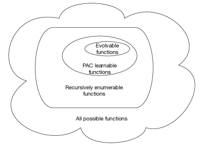
The fundamental question addressed in Valiant’s evolvability model relate to whether complex functions of many arguments can be evolved in a “reasonable" amount of time with a finite population of variants playing an evolutionary UIG. The definition of what constitutes “reasonable" is of course subjective, but computational learning theory models typically posit that models that use polynomial amount of resources in the parameters of interest, such as the size of the representation used to encode the function or the training experience, are reasonable, and distinguish them from those that consume a non-polynomial amount of resources. Leaving aside the tricky question of whether what is computable by a Turing machine or a digital computer necessarily translates into what is feasible in biology or physics (which operate according to the principles of quantum mechanics Coecke and Kissinger (2017)), let us consider this model to begin with to provide an initial analysis of the differences between evolvability and learnability.
If we restrict our attention to monotone conjunctions, and define a target function as some subset of literatus . denotes the possible arguments that the variables can take. Let denote a probability distribution over . We can interpret a “target" function as the “teacher" and any guess about as a “participant" trying to “imitate" the teacher.
Definition 89.
The performance of a participant in an evolutionary UIG with respect to a “teacher participant for a given probability distribution over is defined as
In simple terms, is simply measuring the correlation between the teacher and the learner. The basic model posits that every time the participant has an experience in the form of a set of values , it will receive a “benefit" of if its “circuit" agrees with the teacher’s “circuit" on that , and receive a penalty if it disagrees. Over a sequence of experiences over a “lifetime", the total of all benefits and penalties are accumulated. Organisms that have a high benefit will be preferentially selected for “reproduction" through imitation (or “cloning") over those that have lower benefits. A large number of variations of this model have been studied in the evolutionary dynamics literature Novak (2006). The function is an example of a fitness landscape Beerenwinkel et al. (2006).
If we restrict ourselves to the very constrained class of monotone conjunctions, and the target teacher participant’s behavior is described by some specific conjunction, say , then the goal of the learner participant is to evolve its behavior to match that of the teacher. It can do so by essentially deleting or adding a single literal, which can be viewed as a toy example of actual evolution on the genomic structure of an organism. In Valiant’s framework, it can be shown that some classes of boolean functions are evolvable, such as monotone conjunctions, whereas others such as the parity function is not evolvable (from a uniform distribution on ). We will not discuss the specifics of this particular proposal modeling evolvability as it involves making many possibly ad-hoc assumptions on the nature of evolution, and the ultimate conclusion that evolvability is s subclass of learnabiilty might strike some as too limiting a notion. In biology, evolution seems capable of remarkable abilities, as it clearly has evolved rather complex creatures such as ourselves. Whether this is a function of purely a process that is even simpler than machine learning processes like gradient descent is a topic for debate that is beyond the scope of this paper.
4.2 Evolutionary UIGs in categories
To model the process of evolution as a search in a fitness landscape, we need to make assumptions on the structure of the space that the fitness landscape is defined over. In Valiant’s model that was just discussed, the fitness landscape was boolean assignments over variables. Other approaches that have been studied include modeling fitness landscapes over distributed lattices Beerenwinkel et al. (2006), graphs Novak (2006), and in the vast literature on genetic programming, the fitness landscape is defined over the set of all programs (e.g., LISP programs in Koza’s work Koza (1992)). A complete discussion of the merits of each such approach is beyond the scope of this paper. Rather, we want to focus our discussion specifically on the advantages of using category theory to formulate the problem of modeling fitness landscapes. We begin by considering the problem in some of the categories described above in Sections 2 and Section 3.
Evolutionary UIGs in Universal Coalgebras
We saw above that universal coalgebras Jacobs (2016); Rutten (2000); Sokolova (2011) provide a rich language for defining dynamical systems and stochastic processes. We can adapt the models of evolutionary dynamics proposed in the literature to the setting of coalgebras relatively easily. To make this more concrete, we begin with the simple example of evolutionary dynamics over Moran processes Moran (1958).
The Moran process is a stochastic model that is widely used to study evolution in finite populations Lieberman et al. (2005). To illustrate this process as it applies to evolutionary UIGs, let us define a population of participants of a constant size , who are comprised of two types of individuals. For example, in the setting of understanding how novel technologies spread through an economy, let us imagine that there are two types of businesses: those who have adopted generative AI in their products, indicated by blue, and those who have yet to adopt generative AI, indicated by red.
The Moran process is a classic example of a stochastic process that is driven by a simple Markov chain, which can be simply defined as a triangular stochastic matrix Lieberman et al. (2005). At each step in the process, a single participant is selected for reproduction. Under the somewhat unrealistic assumption that the population size remains constant, it is necessary therefore that some participant has to go extinct. We can imagine that at each step, one company that has adopted generative AI is allowed to reproduce, but another that failed to adopt generative AI goes out of business. Participants that are selected for reproduction and extinction are chosen randomly. The blue and red participants have different finesses that in turn change the rates at which they reproduce. If the fitness of type red is normalized to the value , and the fitness of type blue is set to , then the probability that type blue is chosen to reproduce is given by
assuming there are individuals of type blue, and individuals of type red. This implies that the probability that participants of type red are chosen to reproduce is given by
In Figure 31, blue individuals have a relative fitness of , and their sizes are proportional to their relative fitness. At the beginning, the population has fewer blue dots (indicating fewer companies have embraced generative AI), and at the end of the evolutionary process, all companies have incorporated generative AI. Those that did not have gone bankrupt, and are not shown in this illustration.
It is relatively simple to design a universal coalgebra over a distribution functor to capture a Moran process, defined coalgebraically as
where maps a set to a probability distribution over that defines each step of the Moran process. We can in fact relatively straightforwardly design a whole family of coalgebraic Moran processes, building on the library of stochastic coalgebras defined in Sokolova (2011). It is also immediate that the final coalgebra here is defined by one of two recurrent states, where the population of participants is all of the same type (either all red or all blue dots in Figure 31), after which no further changes will be possible.
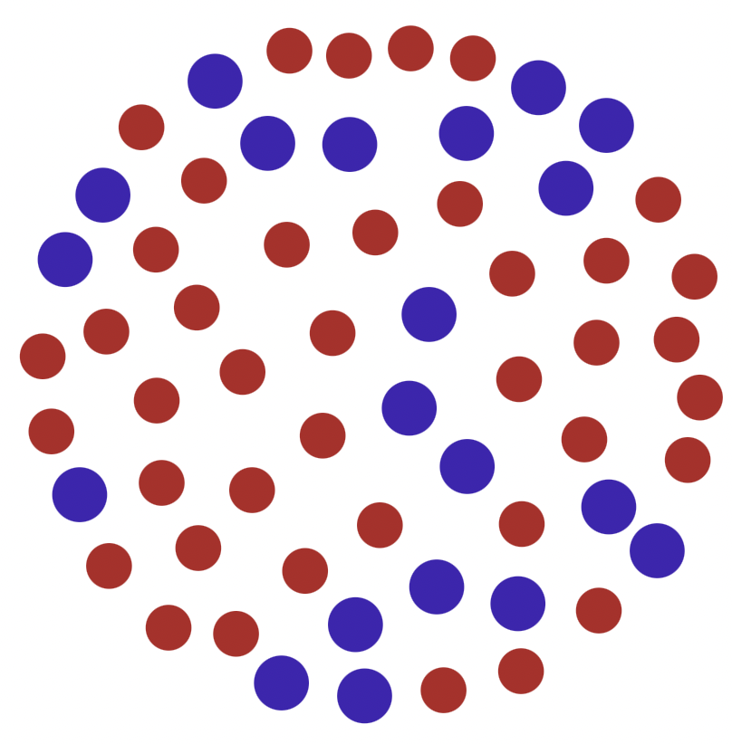
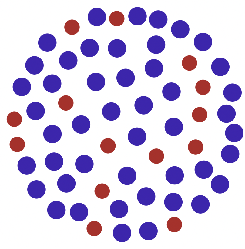

4.3 Evolutionary UIGs in Finite Topological Spaces: A Bioinformatics Example
A fundamental aspect of fitness landscape modeling in evolutionary UIGs is to assume that a participant’s behavior is a function of its genomic structure that is largely based on the set of mutations that it has accumulated over time. That is, mutations are irreversible and we can define a category structure (such as a partial order) that specifies constraints on the order in which mutations have ocurred. We now summarize some previous work of ours Mahadevan (2021a) that explored construction of topological causal models from genomic cancer data, where the topological structure essentially defines a type of category. In other words, when we use the word “topological causal model" in this section, it should be interpreted as a finite category defined by a partial order.
| Tumor | Gene |
|---|---|
| Pa017C | KRAS |
| Pa017C | TP53 |
| Pa019C | KRAS |
| Pa022C | KRAS |
| Pa022C | SMAD4 |
| Pa022C | TP53 |
| Pa032X | CDKN2A |
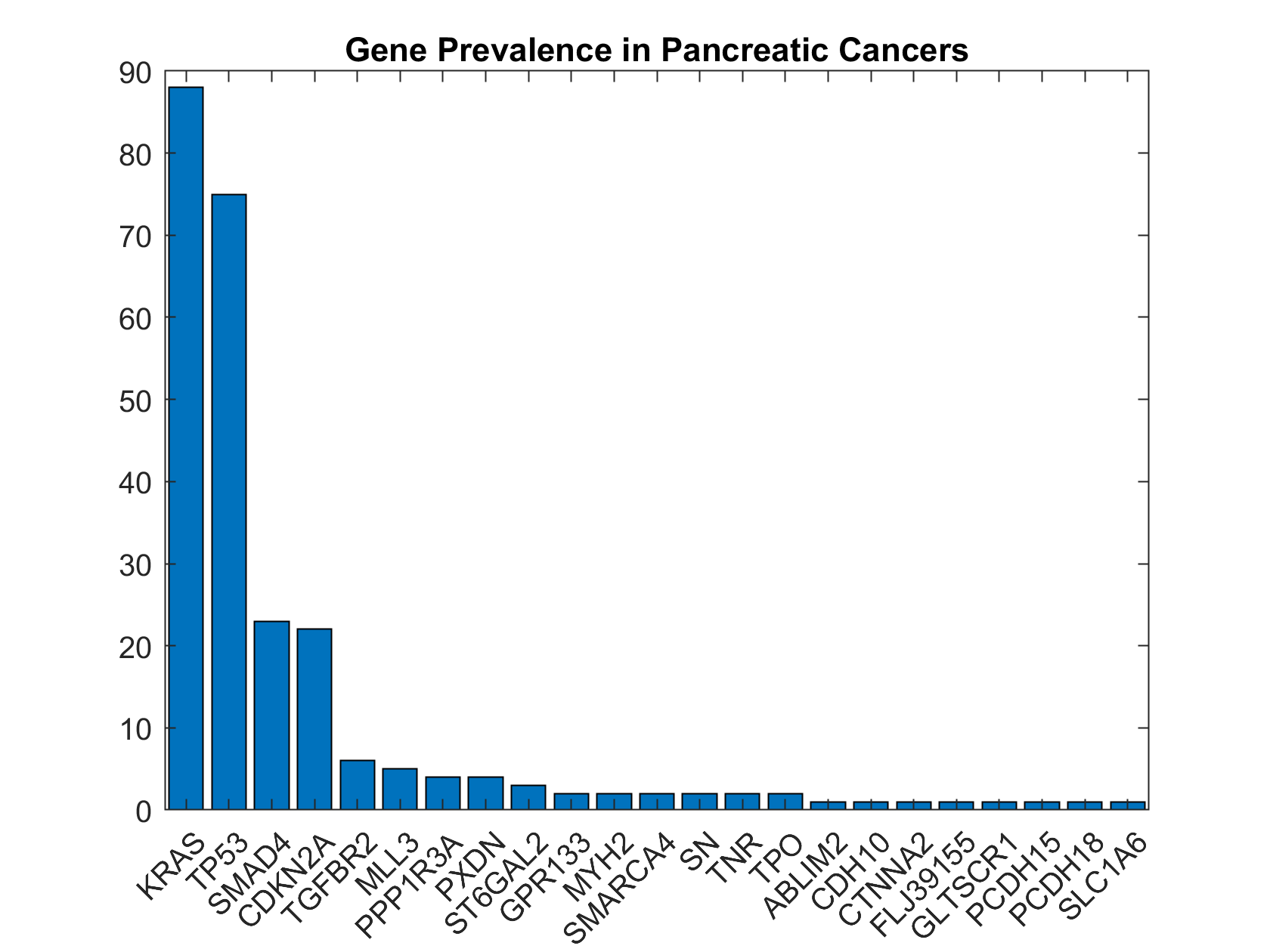
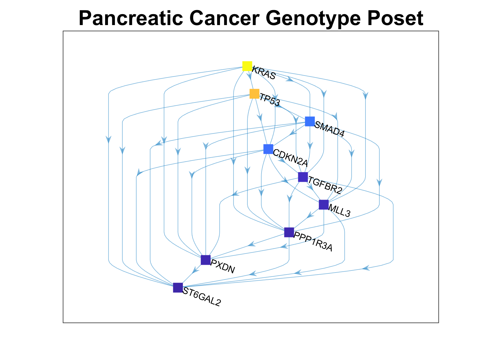
Table 32 shows a small fragment of a dataset for pancreatic cancer (Jones et al., 2008). Like many cancers, it is marked by a particular partial ordering of mutations in some specific genes, such as KRAS, TP53, and so on. In order to understand how to model and treat this deadly disease, it is crucial to understand the inherent partial ordering in the mutations of such genes. Pancreatic cancer remains one of the most prevalent and deadly forms of cancer. Roughly half a million humans contract the disease each year, most of whom succumb to it within a few years. Figure 33 shows the roughly most common genes that undergo mutations during the progression of this disease. The most common gene, the KRAS gene, provides instructions for making a protein called K-Ras that is part of a signaling pathway known as the RAS/MAPK pathway. The protein relays signals from outside the cell to the cell’s nucleus. The second most common mutation occurs in the TP53 gene, which makes the p53 protein that normally acts as the supervisor in the cell as the body tries to repair damaged DNA. Like many cancers, pancreatic cancers occur as the normal reproductive machinery of the body is taken over by the cancer.
In the pancreatic cancer problem, for example, the topological space is comprised of the significant events that mark the progression of the disease, as shown in Table 33. In particular, the table shows that specific genes are mutated at specific locations by the change of an amino acid, causing the gene to malfunction. We can model a tumor in terms of its genotype, namely the subset of , the gene events, that characterize the tumor. For example, the table shows the tumor Pa022C can be characterized by the genotype KRAS, SMAD4, and TP53. In general, a finite space topology is just the elements of the space (e.g. genetic events), and the subspaces (e.g., genomes) that define the topology.
We can now define the problem as one of inferring topological causal models for cancer (Beerenwinkel and Sullivant, 2009; Beerenwinkel et al., 2007, 2006; Gerstung et al., 2011), which define a simple type of categorical structure. The progression of many types of cancer are marked by mutations of key genes whose normal reproductive machinery is subverted by the cancer (Jones et al., 2008). Often, viruses such as HIV and COVID-19 are constantly mutating to combat the pressure of interventions such as drugs, and successful treatment requires understanding the partial ordering of mutations. A number of past approaches use topological separability constraints on the data, assuming observed genotypes separate events, which as we will show, is abstractly a separability constraint on the underlying topological space.
| Regulatory pathway | % altered genes | Tumors | Representative altered genes |
|---|---|---|---|
| Apoptosis | 9 | 100% | CASP10, VCP, CAD, HIP1 |
| DNA damage control | 9 | 83% | ERCC4, ERCC6, EP300, TP53 |
| G1/S phase transition | 19 | 100% | CDKN2A, FBXW7, CHD1, APC2 |
| Hedgehog signaling | 19 | 100% | TBX5, SOX3, LRP2, GLI1, GLI3 |
| Homophilic cell adhesion | 30 | 79% | CDH1, CDH10, CDH2, CDH7, FAT |
| Integrin signaling | 24 | 67% | ITGA4, ITGA9, ITGA11, LAMA1 |
| c-Jun N-terminal kinase | 9 | 96% | MAP4K3, TNF, ATF2, NFATC3 |
| KRAS signaling | 5 | 100% | KRAS, MAP2K4, RASGRP3 |
| Regulation of invasion | 46 | 92% | ADAM11, ADAM12, ADAM19 |
| Small GTPase–dependent | 33 | 79% | AGHGEF7, ARHGEF9, CDC42BPA |
| TGF- signaling | 37 | 100% | TGFBR2, BMPR2, SMAD4, SMAD3 |
| Wnt/Notch signaling | 29 | 100% | MYC, PPP2R3A, WNT9A |
A key computational level in making model discovery tractable in evolutionary processes, such as pancreatic cancer, is that multiple sources of information are available that guide the discovery of the underlying poset model. In particular, for pancreatic cancer (Jones et al., 2008), in addition to the tumor genotype information show in Table 33, it is also known that the disease follows certain pathways, as shown in Table 7. This type of information from multiple sources gives the ability to construct multiple posets that reflect different event constraints (Beerenwinkel et al., 2006). Algorithm 1 is a generalization of past algorithms that infer conjunctive Bayesian networks (CBN) from a dataset of events (e.g., tumors or signaling pathways) and their associated genotypes (e.g., sets of genes) (Beerenwinkel et al., 2007, 2006) The pathway poset and DAG shown in Figure 33 were learned using Algorithm 1 using the pancreatic cancer dataset published in (Jones et al., 2008).
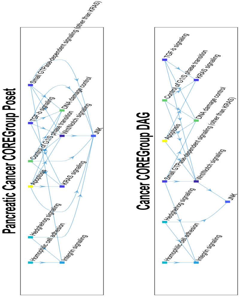
4.4 Game Theory and Variational Inequalities
Having covered some of the basics in evolutionary dynamics, we now introduce the basics of game theoretic models. Our goal is to integrate these, and in particular, we want to focus on variational inequality models (VIs) that generalize classic game-theoretic models. Game theory was pioneered by von Neumann and Morgenstern von Neumann and Morgenstern (1947), and later extended by Nash Nash (1951). An excellent modern overview of game theory is given in Maschler et al. (2013). Game theory has found countlessa applications in many fields, ranging from network economics Nagurney (1999) to algorithmic game theory in computer science Nisan et al. (2007a). Our aim in this section is to illustrate the use of category theory in developing a framework for evolutionary UIGs, principally combining ideas from traditional game theory, network economics, and evolutionary game theory Lieberman et al. (2005). One way to relate this section to the previous is that humans, the target of an imitation game, are the result of millions of years of evolution. In building an AI system that is intended to match humans at imitation games, the role of evolutionary processes cannot be ignored, and in fact, may provide an elegant avenue to building more robust generative AI systems. We saw in the previous section that there are intrinsic limitations on the power of machine learning, which limit the ability of generative AI systems like LLMs at solving even relatively simple classes of tasks Delétang et al. (2023). Perhaps bringing in an evolutionary perspective will help transcend some of these limitations, as it has in biology.
A finite, -person normal form game is a tuple , where is a finite set of players indexed by , is the joint action space formed from the set actions available to each player (), and is a tuple of the players’ utility functions (or payoffs) where . The difficulty in computing the equilibrium depends on the constraints placed on the game. For instance, two-player, zero-sum games, ensure that player interests are diametrically opposed and can thus be formulated as linear programs (LPs) by the minmax theorem and solved in polynomial time Shoham and Leyton-Brown (2008).
By contrast, in two-player, general-sum games, any increase in one player’s utility does not necessarily result in a decrease in the other player’s utility so a convenient LP formulation is not possible. Finding Nash equilibria in two-player, general-sum games is thought to be time exponential in the size of the game in the worst case. It has been shown that every game has at least one Nash equilibrium which delegates the problem to the class PPAD (polynomial parity argument, directed version) originally designated by Papadimitriou Papadimitriou (2001). Although this game type cannot be converted to an LP, it can be formulated as a linear complimentarily problem (LCP). In crude terms, the LCP can be formed by introducing an additional constraint called a complementarity condition to the combination of constraints that would appear in each agent’s LP had it only been a zero-sum game. Unlike the LP, the LCP is only composed of constraints making it a pure constraint satisfaction problem (CSP). The most popular game theoretic algorithm for solving these LCPs is the Lemke-Howson algorithm Lemke and Howson (1964). This algorithm performs a series of pivot operations that swap out player strategies until all constraints are satisfied. An alternate approach is to employ heuristics as in the case of the support-enumeration method (SEM) which repeatedly tests whether a Nash equilibrium exists given a pair of actions, or support profile. The heuristic used is to favor testing smaller, more balanced support profiles in order to prune larger regions of the action space.
Finally, we encounter n-player, general-sum games, in which the complementarity problem previously defined is now nonlinear (NCP). One common approach is to approximate the solution of the NCP as solving a sequence of LCPs (SLCP). This method is typically fast, however, it is not globally convergent. Another technique is to solve an optimization problem in which the global minima equate to the Nash equilibria of the original problem. The drawback is that there are local minima that do not correspond to Nash equilibria making global convergence difficult. Several other algorithms for solving n-player, general-sum games exist as well including a generalized SEM but also simplical subdivision algorithms Van der Laan et al. (1987), the Govindan-Wilson method Govindan and Wilson (2003), and other homotopy methods.
Some games exhibit a characteristic of payoff independence where a single player’s payoff is dependent on only a subset of the other players in the game. In this case, the reward table indexed by the joint action-space of all players is overly costly prompting a move from the normal form representation of the game to the more compact representation offered by graphical games. This can often reduce the space of the representation from exponential to polynomial in the number of players. When the graph is a tree, a commonly used method, NashProp, computes an -Nash equilibrium with a back and forth sweep over the graph from the leaves to the root.
Still other representations and methods exist for extensive-form games, however, we will limit our focus here to normal-form games. There is also a large body of work on the convergence to Nash equilibria in the multi-agent reinforcement learning (MARL) setting Busoniu et al. (2008); Abdallah and Lesser (2008); Singh et al. (2000) that we will not explore in this paper. A discussion of the approaches above and more on the computation of equilibria in games can be found in Shoham and Leyton-Brown (2008); Von Stengel (2002); McKelvey and McLennan (1996).
There has been previous work on using category theory to model games, which has been referred to as open games due to its compositional nature Ghani et al. (2018); Hedges (2017). The basic framework adopted here is to define games as a symmetric monoidal category, where the compositional structure permits the transmission of utilities backwards, and permits games to be composed. It is an elegant approach, but differs from our primary motivation of incorporating evolutionary birth-death processes into game theory. Fundamentally, evolution causes players in a game to be eliminated, which is an aspect of all real-life competitive games, from chess competitions to the Olympics, and competitive sports of any kinds features elimination tournaments. It is also a reality in the business world that companies that do not adapt to market changes go bankrupt and are no longer viable players in a network economy. To model such processes, we need to include additional components that are not in the open games formalism, although as we show below, they could be included in such categorical formulations of games.
Stochastic Variational Inequalities
We now introduce classical variational inequalities (VIs) Facchinei and Pang (2003), and outline a metric coinduction type algorithm for stochastic VIs based on Alfredo N. Iusem (2018); Wang and Bertsekas (2015). VIs generalize both classical game theory as well as optimization problems, in that any (convex) optimization problem or any Nash game can be formulated as a VI, but the converse is not true. More precisely, a variational inequality model VI(), where is a collection of modular vector-valued functions defined as , where , with each being a convex domain such that .
Definition 90.
The category of VIs is defined as one where each object is defined as a finite-dimensional variational inequality problem = VI(, where the vector-valued mapping is a given continuous function, is a given closed convex set, and is the standard inner product in , and the morphisms from one object to another correspond to non-expansive functions. Solving a VI is defined as finding a vector such that
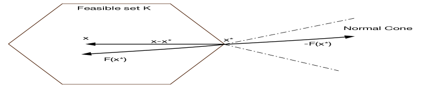
We can also define a category of stochastic VIs as follows. In the stochastic case, we start with a measurable space , a measurable random operator , and a random variable defined on a probability space , which enables defining the usual notions of expectation and distributions of .
Definition 91.
The category of stochastic VIs is defined as one where each object is defined as a finite-dimensional stochastic variational inequality problem = SVI(, where the vector-valued mapping is given by for all .
4.5 Example of VI: Network Economics of Generative AI
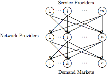
We can use the framework of category theory to also analyze complex network economies that are built on top of generative AI systems. Generative AI systems offer cloud computing services to users geographically dispersed around the world. They charge for these services based on factors such as the number of tokens processed in a large language model, or the number of images rendered using a diffusion model. These services incur significant costs for the vendors of generative AI models. A fundamental principle of network economics is that for successful trade to occur, there must be an equilibrium principle that is satisfied on the network between the producers, the transporters who control the “plumbing" of the network itself, and the users who form the demand market for the generative AI services. In other words, the producers selling cloud computing generative AI services must be able to earn sufficient money by selling their products to continue to offer them. The users who must both pay for the generative AI services and for using the transport network choose the best combination of generative AI producer and network transporter that is within their budget.
Formally, it can be shown that the network economics of generative AI is an example of a broad class of mathematical problems called variational inequalities (VIs) Nagurney (1999); Facchinei and Pang (2003). A novel aspect of our paper is the use of category theory, in particular universal coalgebras, to model VIs, and the use of this framework to model the network economics of generative AI. The solution to a VI is unique, under the following conditions, where is compact and is continuous.
Definition 92.
is monotone if , .
Definition 93.
is strongly monotone if .
Definition 94.
is Lipschitz if .
We now describe how to model causal inference in a network economics problem, which will be useful in illustrating the abstract definitions from the previous section. The model in Figure 36 is drawn from Nagurney (1999); Nagurney and Wolf (2014). which were deterministic, and included no analysis of causal interventions. This network economics model comprises of three tiers of agents: producer agents, who want to sell their goods, transport agents who ship merchandise from producers, and demand market agents interested in purchasing the products or services. The model applies both to electronic goods, such as video streaming, as well as physical goods, such as face masks and other PPEs. Note that the design of such an economic network requires specifying the information fields for every producer, transporter and consumer. For the sake of brevity, we assume that the definition of these information fields are implicit in the equations defined below, but a fuller discussion of this topic will be studied in a subsequent paper.
The model assumes service providers, network providers, and demand markets. Each firm’s utility function is defined in terms of the nonnegative service quantity (Q), quality (q), and price () delivered from service provider by network provider to consumer . Production costs, demand functions, delivery costs, and delivery opportunity costs are designated by , , , and respectively. Service provider attempts to maximize its utility function by adjusting (eqn. 11a). Likewise, network provider attempts to maximize its utility function by adjusting and (eqn. 11b).
| (11a) | ||||
| (11b) | ||||
We assume the governing equilibrium is Cournot-Bertrand-Nash and the utility functions are all concave and fully differentiable. This establishes the equivalence between the equilibrium state we are searching for and the variational inequality to be solved where the mapping is a vector consisting of the negative gradients of the utility functions for each firm. Since is essentially a concatenation of gradients arising from multiple independent, conflicting objective functions, it does not correspond to the gradient of any single objective function.
| (12a) | ||||
| where | ||||
| and | ||||
| (12b) | ||||
| (12c) | ||||
| (12d) | ||||
The variational inequality in Equations 12a represents the result of combining the utility functions of each firm into standard form. is derived by taking the negative gradient of with respect to . is derived by taking the negative gradient of with respect to . And is derived by taking the negative gradient of with respect to .
4.5.1 Numerical Example
We extend the simplified numerical example in Nagurney and Wolf (2014) by adding stochasticity to illustrate our causal variational formalism. Let us assume that there are two service providers, one transport agent, and two demand markets. Define the production cost functions:
where are random variables indicating errors in the model. Similarly, define the demand price functions as:
Finally, define the transportation cost functions as:
and the opportunity cost functions as:
Using the above equations, we can easily compute the component mappings as follows:
For simplicity, we have not indicated the noise terms above, but assume each component mapping has an extra noise term . For example, if we set the network service cost of network provider 1 serving the content producer 1 to destination market 1 to 0, then the production cost function under the intervention distribution is given by
Finally, the Jacobian matrix associated with is given by the partial derivatives of each mapping with respect to is given as:
Note this Jacobian is non-symmetric, but positive definite, as it is diagonally dominant. Hence the induced vector field can be shown to be strongly monotone, and the induced VI has exactly one solution.
Crucially, VI problems can only be converted into equivalent optimization problems when a very restrictive condition is met on the Jacobian of the mapping , namely that it be symmetric. Most often, real-world applications of VIs do not induce symmetric Jacobians.
Theorem 27.
Assume is continuously differentiable on and that the Jacobian matrix of partial derivatives of with respect to (w.r.t) each is symmetric and positive semidefinite. Then there exists a real-valued convex function satisfying with , the solution of VI(F,K), also being the mathematical programming problem of minimizing subject to .
The algorithmic development of methods for solving VIs begins with noticing their connection to fixed point problems.
Theorem 28.
The vector is the solution of VI(F,K) if and only if, for any , is also a fixed point of the map , where is the projector onto convex set .
In terms of the geometric picture of a VI, the solution of a VI occurs at a vector where the vector field induced by on is normal to the boundary of and directed inwards, so that the projection of is the vector itself. This property forms the basis for the projection class of methods that solve for the fixed point.
With this insight, we can define a category of coalgebras over VIs, where the endofunctor is defined in terms of the vector field as defined above, and the solution to the VI corresponds to finding the final coalgebra representing the solution to the VI problem. Together, the VI and PDS frameworks provide a mathematically elegant approach to modeling and solving equilibrium problems in game theory Fudenberg and Levine (1998); Nisan et al. (2007b). A Nash game consists of players, where player chooses a strategy belonging to a closed convex set . After executing the joint action, each player is penalized (or rewarded) by the amount , where is a continuously differentiable function. A set of strategies is said to be in equilibrium if no player can reduce the incurred penalty (or increase the incurred reward) by unilaterally deviating from the chosen strategy. If each is convex on the set , then the set of strategies is in equilibrium if and only if . In other words, needs to be a solution of the VI , where .
Two-person Nash games are closely related to saddle point optimization problems Juditsky et al. (2011a, b); Liu et al. (2012) where we are given a function , and the objective is to find a solution such that
| (13) |
Here, is convex in for each fixed , and concave in for each fixed .
The class of complementarity problems can also be reduced to solving a VI. When the feasible set is a cone, meaning that if , then , then the VI becomes a CP.
Definition 95.
Given a cone and mapping , the complementarity problem CP(F,K) is to find an such that , the dual cone to , and . 444Given a cone , the dual cone is defined as .
The nonlinear complementarity problem (NCP) is to find (the non-negative orthant) such that and . The solution to an NCP and the corresponding are the same, showing that NCPs reduce to VIs. In an NCP, whenever the mapping function is affine, that is , where is an matrix, the corresponding NCP is called a linear complementarity problem (LCP) Murty (1988).
4.6 A Metric Coinduction Algorithm for solving VIs
We now discuss algorithms for solving VI’s. There are a wealth of existing methods for deterministic VI’s (Facchinei and Pang, 2003; Nagurney, 1999)). First, we present a few of the standard algorithms used to compute solutions to variational inequalities and equilibria in projected dynamical systems. We finally describe an adaptation of a stochastic approximation method Robbins and Monro (1951) to solve VIs, which can be viewed as a special type of metric coinduction method.
The basic projection-based method (Algorithm 1) is as follows:
Here, is the orthogonal projector onto the convex set . It can be shown that the basic projection algorithm solves any for which the mapping is strongly monotone and Lipschitz smooth. A simple strategy is to set where , is the Lipschitz smoothness constant, and is the strong monotonicity constant. Setting equal to a constant in this manner recovers what is known as Euler’s method and is the most basic algorithm for solving both VIs and PDS.
The basic projection-based algorithm has two critical limitations. First, it requires that the mapping be strongly monotone. If, for example, is the gradient map of a continuously differentiable function, strong monotonicity implies the function must be strongly convex. Second, setting the parameter requires knowing the Lipschitz smoothness and the strong monotonicity parameter .
Korpelevich (1977) extended the projection algorithm with the well-known “extragradient" method, which requires two projections, but is able to solve VI’s for which the mapping is only monotone. The key idea behind the extragradient method is to use the F mapping evaluated at the result of the projection method, , instead of . In other words, step 3 of Algorithm 2 is replaced with
| Set | |||
| Set |
Gemp et al. (2015) proposed a more sophisticated extragradient algorithm, combining Runge-Kutta methods from ODE’s with a modified dual-space mirror-prox method to solve large network games modeled as VI’s, such as the network economy shown in Figure 36, but required multiple projections corresponding to the order of the Runge-Kutta approximation. If projections are expensive, particularly in large network economy models, these algorithms may be less attractive than incremental stochastic projection methods, which we turn to next.
Convergence Analysis of VI Algorithms
At the heart of convergence analysis of any VI method is bounding the iterates of the algorithm. In the below derivation, represents the final solution to a VI, and , are successive iterates:
Here, the first inequality follows from the nonexpansive property of projections, and the last inequality follows from strong monotonicity and Lipschitz property of the mapping. Bounding the term is central to the design of any VI method.
A Stochastic Approximation Method for Stochastic VIs
We now describe an incremental two-step projection method for solving (stochastic) VI’s, which is loosely based on Wang and Bertsekas (2015); Alfredo N. Iusem (2018). The general update equation can be written as:
| (14) |
where and are sequences of random variables, generated by sampling a VI model, and and are sequences of positive scalar step sizes. Note that an interesting feature of this algorithm is that the sequence of iterates is not guaranteed to remain within the feasible space at each iterate. Indeed, represents the projection onto a randomly sampled constraint .
The analysis of convergence of this algorithm is somewhat intricate, and we will give the broad highlights as it applies to stochastic VI’s. Define the set of random variables . Similar to the convergence of the projection method, it is possible to show that the error of each iteration is stochastically contractive, in the following sense:
where are positive errors such that and . Note that the assumption of stochastic contraction is essentially what makes this algorithm an example of metric coinduction Kozen and Ruozzi (2009). The convergence of this method rests on the following principal assumptions, stated below:
Theorem 1.
The mapping is strongly monotone, and the sampled mapping is stochastically Lipschitz continuous with constant , namely:
| (15) |
Theorem 2.
The mapping is bounded, with constant such that
| (16) |
Theorem 3.
The distance between each iterate and the feasible space reduces “on average", namely:
| (17) |
where and is a finite set of indices such that .
Theorem 4.
where .
Theorem 5.
Supermartingale convergence theorem: Let denote the collection of nonnegative random variables from
| (18) |
and and w.p. 1. Then, converges to a nonnegative random variable, and .
Theorem 6.
The random variables are such that for
namely, the individual constraints will be sampled sufficiently. Also, the sampling of the stochastic components ensures that
Given the above assumptions, it can be shown that two-step stochastic algorithm given in Equation 14 converges to the solution of a (stochastic) VI.
Theorem 29.
Given a finite-dimensional stochastic variational inequality problem is defined by a model = SVI(, where , where now denotes expectation, the two-step algorithm given by Equation 14 produces a sequence of iterates that converges almost surely to , where
Proof: The proof of this theorem largely follows the derivation given in (Alfredo N. Iusem, 2018; Wang and Bertsekas, 2015). ∎
To reiterate, these stochastic approximation methods for solving (stochastic) VIs are essentially instances of the more general metric coinduction framework Kozen and Ruozzi (2009), and the key to understanding them from a category-theoretic framework is to formulate them in the context of finding final coalgebras given by the fixed point equation that solves a given (stochastic) VI.
Evolutionary Imitation Games with VIs
Finally, we can adapt the VI algorithms described above to the evolutionary setting by inserting in a “mutation" component where at each step of the evolutionary process, some participant in a network economy goes “extinct" and is replaced with another participant who is more “fit". Following the similar strategy used in the discussion of Moran processes above, we can analyze the convergence of such a network economy where participants are randomly selected for extinction and replacement. A full analysis of this problem is beyond the scope of this paper, and is a topic for future work, but we give the high-level idea here.
In a standard VI, we are given a vector field , which represents a network economy such as the one illustrated in Figure 36, and the goal is to find the equilibrium of this network economy game. To define an evolutionary network economy game, we now add the “birth-death" stochastic process or the mutation process defined above with Moran processes or with bioinformatics example of genetic mutations, or with Valiant’s evolvability model. That is, we assume that each step of the evolutionary UIG, we have a set of participants playing the network economy game, and we solve that using (for example) the stochastic approximation algorithm described above. Given a solution to the current network economy game, we apply a mutation operator by eliminating one participant (say as in a Moran process), and then reproduce another participant of higher fitness to keep the population size fixed. This evolutionary step might correspond to a business going bankrupt or being bought over by another higher fitness business. The network economy game is then played again, and the process repeats. The convergence of such evolutionary UIGs is a matter of choosing the right type of incremental mutation operator such that the overall process converges. The principle of metric coinduction provides a broad category-theoretic framework to analyze usch evolutionary UIGs.
5 Universal Imitation Games on Quantum Computers
“Nature isn’t classical, dammit, and if you want to make a simulation of nature, you’d better make it quantum mechanical, and by golly it’s a wonderful problem, because it doesn’t look so easy.” – Richard Feynman
Thus far in this paper, we have made an implicit assumption that the solutions to imitation games would be implemented on a classical computer, in particular Turing’s machine. However, the underlying mathematics we have used in analyzing imitation games generalizes elegantly to imitation games that can and will undoubtedly be played in the near future on quantum computers Abramsky and Coecke (2004); Coecke and Kissinger (2017). In this final brief section, we want to give a high level description of quantum UIGs, and what they may imply in terms of strategies for playing imitation games. This possibility is not science fiction. Toumi (2022) gives a detailed description of how to model natural language processing on quantum computers using category theory in his PhD thesis. He also describes the DiScoPy Python programming environment for converting natural language sentences into symmetric monoidal categories. It is quite feasible, perhaps not yet practical, to design algorithms to play quantum imitation games using packages like DisCoPy de Felice et al. (2021), although in the years ahead, it will become increasingly feasible, and perhaps the staggering energy costs of current generative AI software on conventional computers will leave us no choice but to turn to quantum computers to play imitation games.
5.1 Compact Closed Categories
To begin with, we need to define a model of quantum computation, and along the same lines of study that we have undertaken so far. That is, the first question we have to answer is: what is the underlying category that quantum computing is based on? Figure 37 illustrates what can be referred to as a smorgasbord of categories, a very small sampling of the possible ways in which categories can be defined. We give a brief description of compact closed categories, which has been proposed as a category for quantum protocols, such as entanglement Abramsky and Coecke (2004).
Definition 96.
A symmetric monoidal category is defined as a category with a bifunctor , a unit object , and natural isomorphisms
which needs to satisfy some additional coherence conditions as defined in MacLane (1971).
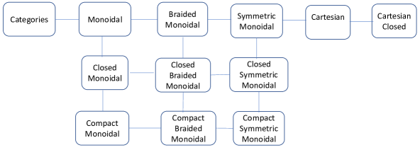
Definition 97.
A category C is *-autonomous if it is a symmetric monoidal category with dual objects represented by a full and faithful functor
satisfying the bijection
that is natural over , , and . A compact closed category is an *-autonomous category with a self-dual tensor operator, satisfying the natural isomorphisms
An alternative way to think of compact closed categories is to view them as a symmetric monoidal category where every object has a dual object, given by , such that it defines a unit
and a counit
satisfying the following commutative diagram:
Example 17.
The monoidal category of sets, relations and Cartesian products is a compact closed category.
Example 18.
The monoidal category of finite-dimensional vector spaces over a field is a compact closed category.
5.2 Quantum Teleportation and Entanglement
We want to briefly sketch out why compact closed categories provide a good categorical representation for quantum UIGs. Our discussion below is based on Abramsky and Coecke (2004). Quantum computing Coecke and Kissinger (2017) is based on modeling the state space of a system as a (finite-dimensional) Hilbert space , which is a finite-dimensional complex vector space with an inner product written in “bra-ket" notation as that is conjugate linear in the first argument and linear in the second. The fact that all computations in an quantum computer are inherently linear is a great advantage, however it is incredibly challenging in almost every other respect, not least of which is the physical challenges associated with preparing an input to a quantum computer, and ensuring that quantum bits (qubits) do not collapse into classical bits while computation is taking place. A quantum state is defined as a one-dimensional subspace of , and represented as a vector of unit norm. Formally, qubits are -dimensional Hilbert spaces, on the basis defined by .
One of the strangest phenomena that occurs in quantum mechanics is entanglement, which arises in compound systems that can be viewed as tensor products of component subsystems and :
where the two subsystems may exhibit correlations that cannot be decomposed into pairs of vectors in each individual subsystem. As a concrete example, illustrated in Figure 38, consider the compound system as represented by two slits through which electrons are shot through Feynman et al. (2010). If one of the two slits is covered, then the probability of the electron being detected at a detector placed at the end opposite from where the electrons are being shot behaves as you would expect. The probability of electrons being detected is highest directly opposite the slit and gradually decays as you move away. However, this behavior which can be easily understood for each subsystem and individually completely changes when both slits are combined in the composite system . Now, there is interference between the two slits and the behavior of the electron changes from being that of a particle to a wave.

All computations in quantum computers are inherently reversible, due to the fact that data transformations are represented as unitary transformations. Given a linear map between two Hilbert spaces, the adjoint is defined as the linear map such that for all and ,
A unitary transformation is a linear isomorphism
satisfying the property that . By tbe bilinearity property, these transformations must preserve inner products
Self-adjoint operators mapping one Hilbert space into another are linear transformations such that . Measurements in quantum computing systems are represented by self-adjoint operators, and can be divided into two phases:
-
1.
An observer receives the outcome of a measurement outcome as a value in the spectrum of the corresponding self-adjoint operator .
-
2.
As a result of the measurement, the state of the system undergoes a change, which can be modeled as the action of a projector whose effect can be understood by a spectral decomposition of the measurement operator
The Born rule states that the probability of does not depend on the value of , but rather on and the state of the system :
To understand the quantum teleportation protocol, let us consider three qubits , and , where is in state , and qubits and are entangled and form an “EPR-pair" with their joint state being . If and are positioned at the source , and is positioned at the target , we perform a Bell-base measurement on and , which means each projects onto one of the one-dimensional subspaces spanned by a vector in the Bell basis:
We can perform a unitary transformation based on the outcome of the measurement, which physically involves transmission of two classical bits, from the location of and to the location of . Quantum teleportation occurs when the final state of is as well. Since a continuous variable has been transmitted, but the actual communication involved the passage of two classical bits, it must be that besides the classical flow of information, there must have been quantum flow of information as well. Abramsky and Coecke (2004) give a detailed analysis of how this type of quantum information flow can be modeled abstractly in a compact closed category, to which we refer the reader for further details. We turn instead to a brief discussion of the issues involved in designing UIG approaches for quantum computing.
5.3 Quantum Coalgebras: Generative AI on Quantum Computers
As we discussed previously in Section 2 and Section 3, generative AI models, from the basic (non)deterministic finite state machine to probabilistic systems to large language models based on neural Vaswani et al. (2017) or dynamical system concepts Gu et al. (2023) can all be viewed as universal coalgebras over some category. We can now consider how to define quantum coalgebras to generalize generative AI over classical computers to quantum computers.
Moore and Crutchfield (2000) define quantum versions of finite-state and push-down automata, as well as regular and context-free grammars. We will follow their treatment below, and then relate it to quantum UIGs.
Definition 98.
A real-time quantum automaton is defined as:
-
1.
A Hilbert space
-
2.
an initial state vector with
-
3.
A subspace and an operator that projects onto it.
-
4.
An input alphabet
-
5.
A unitary transition matrix for each symbol .
Given any string , we can define the quantum language accepted by as the function
which defines a function from strings in to probabilities in . The basic steps in a quantum automaton are to start in the state , apply the unitary matrices for each symbol in in the given order, and measure the probability of the final outcome that the resulting state is in by applying the projection operator , and measuring its resulting norm (which gives us the probability).
To relate it to the discussion of quantum entanglement in the previous section, note that if we have a quantum system that is initially prepared to be a superposition of initial states, and we present it the input string, the matrix product in effect sums over all possible paths that the machine can take (viewed as a stochastic automaton). Each path has a complex amplitude that is given by the product of all the amplitudes of the transitions at each step. The biggest difference from stochastic automata used in generative AI and reinforcement learning is that quantum entanglement will cause destructive interference exactly as illustrated in Figure 38. Paths that have opposite phases in the complex plane can cancel each other out, resulting in a total probability less than the sum of each path, since the amplitude .
Definition 99.
A quantum finite state automaton (QFA) is a quantum automaton where , , and the have finite dimensionality . A quantum regular language(QRL) is a quantum language recognized by a QFA.
Moore and Crutchfield (2000) go on to define quantum analogues of context-free grammars, push-down automata, etc. and explore their properties, to which the reader is referred to for a more in-depth discussion. By suitably defining the category, e.g. Hilbert spaces, and an endofunctor on the category, it is clear that we can define a coalgebra for a quantum finite state automaton (as we can as well for the other generative models in Moore and Crutchfield (2000)). There has been initial work on quantum generative AI systems, such as quantum transformers Cherrat et al. (2022) as well as the work on quantum NLP mentioned earlier Toumi (2022). Fundamentally, to solve a UIG using a quantum computer, we have to define the notion of (weak) isomorphism in each of the cases that we discussed before. We briefly discuss each of these cases.
5.4 Quantum Universal Imitation Games
We proposed using Yoneda embeddings for a participant in a static UIG and determine if two participants are isomorphic based on their Yoneda embeddings. We can generalize the same approach to the quantum computing world by determining quantum Yoneda embeddings in a compact closed category. Following Kelly and Laplaza (1980), we can define compact closed categories as a symmetric monoidal category where every object has a dual object, given by , such that it defines a unit
and a counit
satisfying certain coherence equations given in Kelly and Laplaza (1980).
Definition 100.
Two objects and in a quantum UIG defined as a compact closed category are deemed isomorphic, or if and only if there is an invertible morphism , namely is both left invertible using a morphism so that idX, and is right invertible using a morphism where idY.
What is fundamentally different in the quantum computing world is that computation is now taking place in a compact closed category where objects have duals. As Kelly and Laplaza (1980) define it, a compact closed category is simply a symmetric monoidal category with symmetry isomorphisms in which every object has a left adjoint, and they work out in detail exactly what form this left adjoint takes. An interesting problem for further work is to understand the full consequences of operating in such compact closed categories. We discuss a few sample questions to be explored in further research:
-
•
Causal Inference in Compact Closed Categories: Consider the problem of determining whether two participants in a quantum UIG are isomorphic by doing a series of causal interventions. Although there has been substantial work on causal inference in traditional categories, such as graphs, vector spaces, Hilbert spaces, etc. (see Table 5), we are not aware of any work in causal inference in compact closed categories where objects have duals. This aspect of quantum computing raises many interesting questions that need to be explored. It is worth mentioning as well that causal inference has been explored in the quantum computing world Coecke and Kissinger (2016); Javidian et al. (2022).
-
•
Quantum Machine Learning: There has been substantial work on quantum machine learning Pastorello (2023), including a celebrated algorithm for solving systems of linear equations Harrow et al. (2009). These approaches look very promising due their potentially exponentially lower computational costs, although the broader question of whether there are problems that are provably solvable faster by quantum computers remains an open research question Bernstein and Vazirani (1997). To that end, Bshouty and Jackson (1995) propose an extension of the classic PAC learning framework to the quantum computing world, where they show that the class of all disjunctive normal form (DNF) concepts are efficiently learnable with respect to the uniform distribution by a quantum algorithm using a quantum oracle.
- •
6 Summary
In this paper, we proposed a broad framework for universal imitation games (UIGs), extending Alan Turing’s original proposal from 1950 where participants are to be classified Human or Machine solely from natural language interactions. In our framework, we allow interactions to be arbitrary, and not limited to natural language questions and answers. We also bring to bear mathematics largely developed since Turing – category theory – that involves defining a collection of objects and a collection of composable arrows between each pair of objects that represent “measurement probes" for solving UIGs. We built on on two celebrated results by Yoneda. The first, called the Yoneda Lemma, shows that objects in categories can be identified up to isomorphism solely with measurement probes defined by composable arrows. Yoneda embeddings are universal representers of objects in categories. A simple yet general solution to the static UIG problem, where the participants are not changing during the interactions, is to determine if the Yoneda embeddings are (weakly) isomorphic. In this approach, we are not considering computational constraints, but mainly focusing on formulating the problem in a mathematically general way. The second foundational result of Yoneda from 1960 that we use is an abstract integral calculus defined by coends and ends, which “integrate" out the objects of a category. We illustrated how these unify disparate notions in AI and ML, from distance based approaches to probabilistic generative models. When participants adapt during interactions, we investigated two special cases: in dynamic UIGs, “learners" imitate “teachers". We contrasted the initial object framework of passive learning from observation over well-founded sets using inductive inference – extensively studied by Gold, Solomonoff, Valiant, and Vapnik – with the final object framework of coinductive inference over non-well-founded sets and universal coalgebras, which formalizes learning from active experimentation using causal inference or reinforcement learning. We defined a category-theoretic notion of minimum description length or Occam’s razor based on final objects in coalgebras. Finally, we explored evolutionary UIGs, where a society of participants is playing a large-scale imitation game. Participants in evolutionary UIGs can go extinct from “birth-death" evolutionary processes that model how novel technologies or “mutants" disrupt previously stable equilibria. We ended the paper with a brief discussion of how to play UIGs on quantum computers, a future that looks increasibly likely given the staggering costs of playing imitation games on classical computers. Many directions remain to be pursued in UIGs, and throughout the paper, we sketched out a number of possible avenues that need further study. This paper represents an initial exploration of a fascinating problem, one that will have enormous implications for the future of human society as millions of humans begin to engage in an imitation game with generative AI products.
References
- Abdallah and Lesser (2008) S. Abdallah and V. R. Lesser. A multiagent reinforcement learning algorithm with non-linear dynamics. J. Artif. Intell. Res.(JAIR), 33:521–549, 2008.
- Abramsky and Coecke (2004) S. Abramsky and B. Coecke. A categorical semantics of quantum protocols. In 19th IEEE Symposium on Logic in Computer Science (LICS 2004), 14-17 July 2004, Turku, Finland, Proceedings, pages 415–425. IEEE Computer Society, 2004. doi:10.1109/LICS.2004.1319636. URL https://doi.org/10.1109/LICS.2004.1319636.
- Aczel (1988) P. Aczel. Non-Well-Founded Sets. Csli Lecture Notes, Palo Alto, CA, USA, 1988.
- Adesso (2023) G. Adesso. Towards the ultimate brain: Exploring scientific discovery with chatgpt AI. AI Mag., 44(3):328–342, 2023. doi:10.1002/AAAI.12113. URL https://doi.org/10.1002/aaai.12113.
- Alfredo N. Iusem (2018) P. T. Alfredo N. Iusem, Alejandro Jofré. Incremental constraint projection methods for monotone stochastic variational inequalities. Mathematics of Operations Research, 44(1):236–263, 2018. URL https://doi.org/10.1287/moor.2017.0922.
- Andersson et al. (1997) S. A. Andersson, D. Madigan, and M. D. Perlman. A characterization of Markov equivalence classes for acyclic digraphs. The Annals of Statistics, 25(2):505 – 541, 1997. doi:10.1214/aos/1031833662. URL https://doi.org/10.1214/aos/1031833662.
- Aristotle (1984) Aristotle. The Complete Works of Aristotle, Volumes 1 and 2. Princeton University Press, 1984.
- Asudeh and Giorgolo (2020) A. Asudeh and G. Giorgolo. Enriched Meanings: Natural Language Semantics with Category Theory. Oxford University Press, 09 2020. ISBN 9780198847854. doi:10.1093/oso/9780198847854.001.0001. URL https://doi.org/10.1093/oso/9780198847854.001.0001.
- Avery (2016) T. Avery. Codensity and the giry monad. Journal of Pure and Applied Algebra, 220(3):1229–1251, Mar. 2016. ISSN 0022-4049. doi:10.1016/j.jpaa.2015.08.017. URL http://dx.doi.org/10.1016/j.jpaa.2015.08.017.
- Baez and Stay (2010) J. Baez and M. Stay. Physics, topology, logic and computation: A rosetta stone. In New Structures for Physics, pages 95–172. Springer Berlin Heidelberg, 2010. doi:10.1007/978-3-642-12821-9_2. URL https://doi.org/10.1007%2F978-3-642-12821-9_2.
- Baez et al. (2011) J. C. Baez, T. Fritz, and T. Leinster. A characterization of entropy in terms of information loss. Entropy, 13(11):1945–1957, 2011. ISSN 1099-4300. doi:10.3390/e13111945. URL https://www.mdpi.com/1099-4300/13/11/1945.
- Baldan et al. (2014) P. Baldan, F. Bonchi, H. Kerstan, and B. König. Behavioral metrics via functor lifting, 2014.
- Barwise and Moss (1996) J. Barwise and L. S. Moss. Vicious circles - on the mathematics of non-wellfounded phenomena, volume 60 of CSLI lecture notes series. CSLI, 1996. ISBN 978-1-57586-009-1.
- Beerenwinkel and Sullivant (2009) N. Beerenwinkel and S. Sullivant. Markov models for accumulating mutations. Biometrika, 96(3):645–661, 06 2009. ISSN 0006-3444. doi:10.1093/biomet/asp023. URL https://doi.org/10.1093/biomet/asp023.
- Beerenwinkel et al. (2006) N. Beerenwinkel, N. Eriksson, and B. Sturmfels. Evolution on distributive lattices. Journal of Theoretical Biology, 242(2):409–420, 2006. ISSN 0022-5193. doi:https://doi.org/10.1016/j.jtbi.2006.03.013. URL https://www.sciencedirect.com/science/article/pii/S0022519306001159.
- Beerenwinkel et al. (2007) N. Beerenwinkel, N. Eriksson, and B. Sturmfels. Conjunctive Bayesian networks. Bernoulli, 13(4):893 – 909, 2007. doi:10.3150/07-BEJ6133. URL https://doi.org/10.3150/07-BEJ6133.
- Belkin et al. (2006) M. Belkin, P. Niyogi, and V. Sindhwani. Manifold regularization: a geometric framework for learning from labeled and unlabeled examples. Journal of Machine Learning Research, pages 2399–2434, 2006.
- Bernstein and Vazirani (1997) E. Bernstein and U. Vazirani. Quantum complexity theory. SIAM Journal on Computing, 26(5):1411–1473, 1997. doi:10.1137/S0097539796300921. URL https://doi.org/10.1137/S0097539796300921.
- Bertsekas (2019) D. Bertsekas. Reinforcement Learning and Optimal Control. Athena Scientific, 2019.
- Bertsekas (2022) D. Bertsekas. Lessons from AlphaZero for Optimal, Model Predictive and Optimal Control. Athena Scientific, 2022.
- Bertsekas (2005) D. P. Bertsekas. Dynamic programming and optimal control, 3rd Edition. Athena Scientific, 2005. ISBN 1886529264. URL https://www.worldcat.org/oclc/314894080.
- Boardman and Vogt (1973) M. Boardman and R. Vogt. Homotopy invariant algebraic structures on topological spaces. Springer, Berlin, 1973.
- Bongard (1970) M. M. Bongard. Pattern Recognition. Spartan Books, 1970.
- Bonsangue et al. (1998) M. Bonsangue, F. van Breugel, and J. Rutten. Generalized metric spaces: Completion, topology, and powerdomains via the yoneda embedding. Theoretical Computer Science, 193(1):1–51, 1998. ISSN 0304-3975. doi:https://doi.org/10.1016/S0304-3975(97)00042-X. URL https://www.sciencedirect.com/science/article/pii/S030439759700042X.
- Borceux (1994) F. Borceux. Handbook of Categorical Algebra, volume 1 of Encyclopedia of Mathematics and its Applications. Cambridge University Press, 1994. doi:10.1017/CBO9780511525858.
- Borkar (2008) V. S. Borkar. Stochastic Approximation: A Dynamical Systems Viewpoint. Cambridge University Press, 2008.
- Bradley et al. (2022a) T. Bradley, J. Terilla, and Y. Vlassopoulos. An enriched category theory of language: From syntax to semantics. La Matematica, 1:551–580, 2022a.
- Bradley et al. (2021) T.-D. Bradley, J. Terilla, and Y. Vlassopoulos. An enriched category theory of language: from syntax to semantics, 2021.
- Bradley et al. (2022b) T.-D. Bradley, J. Terilla, and Y. Vlassopoulos. An enriched category theory of language: From syntax to semantics. La Matematica, mar 2022b. doi:10.1007/s44007-022-00021-2. URL https://doi.org/10.1007%2Fs44007-022-00021-2.
- Bshouty and Jackson (1995) N. H. Bshouty and J. C. Jackson. Learning dnf over the uniform distribution using a quantum example oracle. In Proceedings of the Eighth Annual Conference on Computational Learning Theory, COLT ’95, page 118–127, New York, NY, USA, 1995. Association for Computing Machinery. ISBN 0897917235. doi:10.1145/225298.225312. URL https://doi.org/10.1145/225298.225312.
- Busoniu et al. (2008) L. Busoniu, R. Babuska, and B. De Schutter. A comprehensive survey of multiagent reinforcement learning. Systems, Man, and Cybernetics, Part C: Applications and Reviews, IEEE Transactions on, 38(2):156–172, 2008.
- Carlsson and Memoli (2010) G. Carlsson and F. Memoli. Classifying clustering schemes, 2010. URL http://arxiv.org/abs/1011.5270. cite arxiv:1011.5270.
- Castro and Precup (2010) P. S. Castro and D. Precup. Using bisimulation for policy transfer in mdps. In M. Fox and D. Poole, editors, Proceedings of the Twenty-Fourth AAAI Conference on Artificial Intelligence, AAAI 2010, Atlanta, Georgia, USA, July 11-15, 2010, pages 1065–1070. AAAI Press, 2010. doi:10.1609/AAAI.V24I1.7751. URL https://doi.org/10.1609/aaai.v24i1.7751.
- Cattani and Winskel (2005) G. L. Cattani and G. Winskel. Profunctors, open maps and bisimulation. Math. Struct. Comput. Sci., 15(3):553–614, 2005. doi:10.1017/S0960129505004718. URL https://doi.org/10.1017/S0960129505004718.
- Chaitin (2002) G. J. Chaitin. Exploring RANDOMNESS. Discrete mathematics and theoretical computer science. Springer, 2002. ISBN 978-1-85233-417-8.
- Cherrat et al. (2022) E. A. Cherrat, I. Kerenidis, N. Mathur, J. Landman, M. Strahm, and Y. Y. Li. Quantum vision transformers, 2022.
- Coecke (2020) B. Coecke. The mathematics of text structure, 2020.
- Coecke and Kissinger (2016) B. Coecke and A. Kissinger. Categorical quantum mechanics i: Causal quantum processes, 2016.
- Coecke and Kissinger (2017) B. Coecke and A. Kissinger. Picturing Quantum Processes: A First Course in Quantum Theory and Diagrammatic Reasoning. Cambridge University Press, 2017.
- Coecke et al. (2016) B. Coecke, T. Fritz, and R. W. Spekkens. A mathematical theory of resources. Information and Computation, 250:59–86, oct 2016. doi:10.1016/j.ic.2016.02.008. URL https://doi.org/10.1016%2Fj.ic.2016.02.008.
- Cover and Thomas (2006) T. M. Cover and J. A. Thomas. Elements of Information Theory 2nd Edition (Wiley Series in Telecommunications and Signal Processing). Wiley-Interscience, July 2006. ISBN 0471241954.
- Darwin (1876) C. Darwin. The effect of cross and self-fertilization in the vegetable kingdom. John Murray, 1876.
- Dawid (2001) A. P. Dawid. Separoids: A mathematical framework for conditional independence and irrelevance. Ann. Math. Artif. Intell., 32(1-4):335–372, 2001. doi:10.1023/A:1016734104787. URL https://doi.org/10.1023/A:1016734104787.
- de Felice et al. (2021) G. de Felice, A. Toumi, and B. Coecke. Discopy: Monoidal categories in python. Electronic Proceedings in Theoretical Computer Science, 333:183–197, Feb. 2021. ISSN 2075-2180. doi:10.4204/eptcs.333.13. URL http://dx.doi.org/10.4204/EPTCS.333.13.
- Delétang et al. (2023) G. Delétang, A. Ruoss, J. Grau-Moya, T. Genewein, L. K. Wenliang, E. Catt, C. Cundy, M. Hutter, S. Legg, J. Veness, and P. A. Ortega. Neural networks and the chomsky hierarchy. In The Eleventh International Conference on Learning Representations, ICLR 2023, Kigali, Rwanda, May 1-5, 2023. OpenReview.net, 2023. URL https://openreview.net/pdf?id=WbxHAzkeQcn.
- Facchinei and Pang (2003) F. Facchinei and J. Pang. Finite-Dimensional Variational Inequalities and Complementarity Problems. Springer, 2003.
- Fagin et al. (1995) R. Fagin, J. Y. Halpern, Y. Moses, and M. Y. Vardi. Reasoning About Knowledge. MIT Press, 1995. ISBN 9780262562003. doi:10.7551/MITPRESS/5803.001.0001. URL https://doi.org/10.7551/mitpress/5803.001.0001.
- Feynman et al. (2010) R. P. Feynman, R. B. Leighton, and M. Sands. The Feynman lectures on physics; New millennium ed. Basic Books, New York, NY, 2010. URL https://cds.cern.ch/record/1494701. Originally published 1963-1965.
- Feys et al. (2018) F. Feys, H. H. Hansen, and L. S. Moss. Long-Term Values in Markov Decision Processes, (Co)Algebraically. In C. Cîrstea, editor, 14th International Workshop on Coalgebraic Methods in Computer Science (CMCS), volume LNCS-11202 of Coalgebraic Methods in Computer Science, pages 78–99, Thessaloniki, Greece, Apr. 2018. Springer International Publishing. doi:10.1007/978-3-030-00389-0_6. URL https://inria.hal.science/hal-02044650.
- Fong (2012) B. Fong. Causal theories: A categorical perspective on bayesian networks, 2012.
- Fong and Spivak (2018) B. Fong and D. I. Spivak. Seven Sketches in Compositionality: An Invitation to Applied Category Theory. Cambridge University Press, 2018.
- Fritz and Klingler (2023) T. Fritz and A. Klingler. The d-separation criterion in categorical probability. Journal of Machine Learning Research, 24(46):1–49, 2023. URL http://jmlr.org/papers/v24/22-0916.html.
- Fudenberg and Levine (1998) D. Fudenberg and D. K. Levine. The theory of learning in games, 1998.
- Gabriel et al. (1967) P. Gabriel, P. Gabriel, and M. Zisman. Calculus of Fractions and Homotopy Theory. Calculus of Fractions and Homotopy Theory. Springer-Verlag, 1967. ISBN 9780387037776. URL https://books.google.com/books?id=UEQZAQAAIAAJ.
- Gemp et al. (2015) I. Gemp, S. Mahadevan, and B. Liu. Solving large sustainable supply chain networks using variational inequalities. In B. Dilkina, S. Ermon, R. A. Hutchinson, and D. Sheldon, editors, Computational Sustainability, Papers from the 2015 AAAI Workshop, Austin, Texas, USA, January 26, 2015, volume WS-15-06 of AAAI Workshops. AAAI Press, 2015. URL http://aaai.org/ocs/index.php/WS/AAAIW15/paper/view/10122.
- Gerstung et al. (2011) M. Gerstung, N. Eriksson, J. Lin, B. Vogelstein, and N. Beerenwinkel. The temporal order of genetic and pathway alterations in tumorigenesis. PLOS ONE, 6(11):1–9, 11 2011. doi:10.1371/journal.pone.0027136. URL https://doi.org/10.1371/journal.pone.0027136.
- Ghani et al. (2018) N. Ghani, J. Hedges, V. Winschel, and P. Zahn. Compositional game theory, 2018.
- Giry (1982) M. Giry. A categorical approach to probability theory. In Categorical aspects of topology and analysis (Ottawa, Ont., 1980), volume 915 of Lecture Notes in Mathematics, pages 68–85. Springer, Berlin, 1982.
- Gold (1967) E. M. Gold. Language identification in the limit. Information and Control, 10(5):447–474, 1967. ISSN 0019-9958. doi:https://doi.org/10.1016/S0019-9958(67)91165-5. URL https://www.sciencedirect.com/science/article/pii/S0019995867911655.
- Gonçalves (2024) B. Gonçalves. Turing’s test, a beautiful thought experiment. CoRR, abs/2401.00009, 2024. doi:10.48550/ARXIV.2401.00009. URL https://doi.org/10.48550/arXiv.2401.00009.
- Govindan and Wilson (2003) S. Govindan and R. Wilson. A global newton method to compute nash equilibria. Journal of Economic Theory, 110(1):65–86, 2003.
- Gu et al. (2022) A. Gu, K. Goel, and C. Ré. Efficiently modeling long sequences with structured state spaces. In The Tenth International Conference on Learning Representations, ICLR 2022, Virtual Event, April 25-29, 2022. OpenReview.net, 2022. URL https://openreview.net/forum?id=uYLFoz1vlAC.
- Gu et al. (2023) A. Gu, I. Johnson, A. Timalsina, A. Rudra, and C. Ré. How to train your HIPPO: state space models with generalized orthogonal basis projections. In The Eleventh International Conference on Learning Representations, ICLR 2023, Kigali, Rwanda, May 1-5, 2023. OpenReview.net, 2023. URL https://openreview.net/pdf?id=klK17OQ3KB.
- Halpern (2016) J. Y. Halpern. Actual Causality. MIT Press, 2016. ISBN 978-0-262-03502-6.
- Hansen and Ghrist (2020) J. Hansen and R. Ghrist. Opinion dynamics on discourse sheaves, 2020. URL https://arxiv.org/abs/2005.12798.
- Harrow et al. (2009) A. W. Harrow, A. Hassidim, and S. Lloyd. Quantum algorithm for linear systems of equations. Physical Review Letters, 103(15), Oct. 2009. ISSN 1079-7114. doi:10.1103/physrevlett.103.150502. URL http://dx.doi.org/10.1103/PhysRevLett.103.150502.
- Haussler (1987) D. Haussler. Bias, version spaces and valiant’s learning framework. In P. Langley, editor, Proceedings of the Fourth International Workshop on MACHINE LEARNING, pages 324–336. Morgan Kaufmann, 1987. ISBN 978-0-934613-41-5. doi:https://doi.org/10.1016/B978-0-934613-41-5.50036-2. URL https://www.sciencedirect.com/science/article/pii/B9780934613415500362.
- Haussler (1988) D. Haussler. Quantifying inductive bias: AI learning algorithms and valiant’s learning framework. Artif. Intell., 36(2):177–221, 1988. doi:10.1016/0004-3702(88)90002-1. URL https://doi.org/10.1016/0004-3702(88)90002-1.
- Hedges (2017) J. Hedges. Morphisms of open games, 2017.
- Hume (1740) D. Hume. A Treatise of Human Nature. Oxford University Press, 1740.
- Imbens and Rubin (2015) G. W. Imbens and D. B. Rubin. Causal Inference for Statistics, Social, and Biomedical Sciences: An Introduction. Cambridge University Press, USA, 2015. ISBN 0521885884.
- Jacobs (2016) B. Jacobs. Introduction to Coalgebra: Towards Mathematics of States and Observation, volume 59 of Cambridge Tracts in Theoretical Computer Science. Cambridge University Press, 2016. ISBN 9781316823187. doi:10.1017/CBO9781316823187. URL https://doi.org/10.1017/CBO9781316823187.
- Jacobs et al. (2019) B. Jacobs, A. Kissinger, and F. Zanasi. Causal inference by string diagram surgery, 2019.
- Jacques (2023) L. Jacques. Teaching CS-101 at the dawn of chatgpt. Inroads, 14(2):40–46, 2023. doi:10.1145/3595634. URL https://doi.org/10.1145/3595634.
- Javidian et al. (2022) M. A. Javidian, V. Aggarwal, and Z. Jacob. Quantum causal inference in the presence of hidden common causes: An entropic approach. Physical Review A, 106(6), Dec. 2022. ISSN 2469-9934. doi:10.1103/physreva.106.062425. URL http://dx.doi.org/10.1103/PhysRevA.106.062425.
- Jones et al. (2008) S. Jones, X. Zhang, D. W. Parsons, J. C.-H. Lin, R. J. Leary, P. Angenendt, P. Mankoo, H. Carter, H. Kamiyama, A. Jimeno, S.-M. Hong, B. Fu, M.-T. Lin, E. S. Calhoun, M. Kamiyama, K. Walter, T. Nikolskaya, Y. Nikolsky, J. Hartigan, D. R. Smith, M. Hidalgo, S. D. Leach, A. P. Klein, E. M. Jaffee, M. Goggins, A. Maitra, C. Iacobuzio-Donahue, J. R. Eshleman, S. E. Kern, R. H. Hruban, R. Karchin, N. Papadopoulos, G. Parmigiani, B. Vogelstein, V. E. Velculescu, and K. W. Kinzler. Core signaling pathways in human pancreatic cancers revealed by global genomic analyses. Science, 321(5897):1801–1806, 2008. ISSN 0036-8075. doi:10.1126/science.1164368. URL https://science.sciencemag.org/content/321/5897/1801.
- Joyal (2002) A. Joyal. Quasi-categories and kan complexes. Journal of Pure and Applied Algebra, 175(1):207–222, 2002. ISSN 0022-4049. doi:https://doi.org/10.1016/S0022-4049(02)00135-4. URL https://www.sciencedirect.com/science/article/pii/S0022404902001354. Special Volume celebrating the 70th birthday of Professor Max Kelly.
- Joyal et al. (1996) A. Joyal, M. Nielsen, and G. Winskel. Bisimulation from open maps. Information and Computation, 127(2):164–185, 1996. ISSN 0890-5401. doi:https://doi.org/10.1006/inco.1996.0057. URL https://www.sciencedirect.com/science/article/pii/S0890540196900577.
- Juditsky and Nemirovski (2011) A. Juditsky and A. Nemirovski. First order methods for nonsmooth convex large-scale optimization, i: General purpose methods. In Optimization in Machine Learning. MIT Press, 2011.
- Juditsky et al. (2011a) A. Juditsky, A. Nemirovski, et al. First order methods for nonsmooth convex large-scale optimization, i: general purpose methods. Optimization for Machine Learning, pages 121–148, 2011a.
- Juditsky et al. (2011b) A. Juditsky, A. Nemirovski, et al. First order methods for nonsmooth convex large-scale optimization, ii: utilizing problems structure. Optimization for Machine Learning, pages 149–183, 2011b.
- Kan (1958) D. Kan. Adjoint functors. Transactions of the American Mathematical Society, 87(2):294–329, 1958. URL https://doi.org/10.2307/1993102.
- Kearns and Vazirani (1994) M. J. Kearns and U. V. Vazirani. An Introduction to Computational Learning Theory. MIT Press, Cambridge, MA, USA, 1994.
- Kelly (1982) G. Kelly. Basic Concepts of Enriched Category Theory. Cambridge University Press, 1982.
- Kelly and Laplaza (1980) G. Kelly and M. Laplaza. Coherence for compact closed categories. Journal of Pure and Applied Algebra, 19:193–213, 1980. ISSN 0022-4049. doi:https://doi.org/10.1016/0022-4049(80)90101-2. URL https://www.sciencedirect.com/science/article/pii/0022404980901012.
- Kleinberg (2002) J. M. Kleinberg. An impossibility theorem for clustering. In Neural Information Processing Systems, pages 463–470, 2002. URL http://papers.nips.cc/paper/2340-an-impossibility-theorem-for-clustering.
- Korpelevich (1977) G. Korpelevich. The extragradient method for finding saddle points and other problems. Matekon, 13:35–49, 1977.
- Koza (1992) J. R. Koza. Genetic Programming: On the Programming of Computers by Means of Natural Selection. MIT Press, Cambridge, MA, USA, 1992. ISBN 0-262-11170-5.
- Kozen and Ruozzi (2009) D. Kozen and N. Ruozzi. Applications of metric coinduction. Log. Methods Comput. Sci., 5(3), 2009. URL http://arxiv.org/abs/0908.2793.
- Lemke and Howson (1964) C. E. Lemke and J. T. Howson, Jr. Equilibrium points of bimatrix games. Journal of the Society for Industrial & Applied Mathematics, 12(2):413–423, 1964.
- Lewis (1973) D. Lewis. Counterfactuals and comparative possibility. J. Philos. Log., 2(4):418–446, 1973. doi:10.1007/BF00262950. URL https://doi.org/10.1007/BF00262950.
- Lieberman et al. (2005) E. Lieberman, C. Hauert, and M. A. Nowak. Evolutionary dynamics on graphs. Nature, 433(3):312–316, 2005.
- Liu et al. (2012) B. Liu, S. Mahadevan, and J. Liu. Regularized off-policy td-learning. In Advances in Neural Information Processing Systems, pages 836–844, 2012.
- Loregian (2021) F. Loregian. (Co)end Calculus. London Mathematical Society Lecture Note Series. Cambridge University Press, 2021. doi:10.1017/9781108778657.
- Lurie (2009) J. Lurie. Higher Topos Theory. Annals of mathematics studies. Princeton University Press, Princeton, NJ, 2009. URL https://cds.cern.ch/record/1315170.
- MacLane (1971) S. MacLane. Categories for the Working Mathematician. Springer-Verlag, New York, 1971. Graduate Texts in Mathematics, Vol. 5.
- MacLane and leke Moerdijk (1994) S. MacLane and leke Moerdijk. Sheaves in Geometry and Logic: A First Introduction to Topos Theory. Springer, 1994.
- Mahadevan (2021a) S. Mahadevan. Causal homotopy, 2021a. URL https://arxiv.org/abs/2112.01847.
- Mahadevan (2021b) S. Mahadevan. Universal decision models. CoRR, abs/2110.15431, 2021b. URL https://arxiv.org/abs/2110.15431.
- Mahadevan (2022) S. Mahadevan. Categoroids: Universal conditional independence, 2022. URL https://arxiv.org/abs/2208.11077.
- Mahadevan (2023) S. Mahadevan. Universal causality. Entropy, 25(4):574, 2023. doi:10.3390/E25040574. URL https://doi.org/10.3390/e25040574.
- Mahadevan et al. (2014) S. Mahadevan, B. Liu, P. Thomas, W. Dabney, S. Giguere, N. Jacek, I. Gemp, and J. Liu. Proximal reinforcement learning: A new theory of sequential decision making in primal-dual spaces, 2014.
- Maschler et al. (2013) M. Maschler, E. Solan, and S. Zamir. Game Theory. Cambridge University Press, 2013.
- May (1992) J. May. Simplicial Objects in Algebraic Topology. University of Chicago Press, 1992.
- May and Ponto (2012) J. May and K. Ponto. More Concise Algebraic Topology: Localization, Completion, and Model Categories. Chicago Lectures in Mathematics. University of Chicago Press, 2012. ISBN 9780226511788. URL https://books.google.com/books?id=SHhmxUPskFwC.
- McInnes et al. (2018) L. McInnes, J. Healy, and J. Melville. Umap: Uniform manifold approximation and projection for dimension reduction, 2018. URL https://arxiv.org/abs/1802.03426.
- McKelvey and McLennan (1996) R. D. McKelvey and A. McLennan. Computation of equilibria in finite games. Handbook of computational economics, 1:87–142, 1996.
- Mitchell (1977) T. M. Mitchell. Version spaces: A candidate elimination approach to rule learning. In R. Reddy, editor, Proceedings of the 5th International Joint Conference on Artificial Intelligence. Cambridge, MA, USA, August 22-25, 1977, pages 305–310. William Kaufmann, 1977. URL http://ijcai.org/Proceedings/77-1/Papers/048.pdf.
- Moore and Crutchfield (2000) C. Moore and J. P. Crutchfield. Quantum automata and quantum grammars. Theoretical Computer Science, 237(1):275–306, 2000. ISSN 0304-3975. doi:https://doi.org/10.1016/S0304-3975(98)00191-1. URL https://www.sciencedirect.com/science/article/pii/S0304397598001911.
- Moran (1958) P. A. P. Moran. Random processes in genetics. Proceedings of the Cambridge Philosophical Society, 54(1):60–71, 1958.
- Murty (1988) K. Murty. Linear Complementarity, Linear and Nonlinear Programming. Heldermann Verlag, 1988.
- Nagurney (1999) A. Nagurney. Network Economics: A Variational Inequality Approach. Kluwer Academic Press, 1999.
- Nagurney and Wolf (2014) A. Nagurney and T. Wolf. A cournot–nash–bertrand game theory model of a service-oriented internet with price and quality competition among network transport providers. Computational Management Science, 11(4):475–502, 2014.
- Nash (1951) J. Nash. Non-cooperative games. Annals of Mathematics, 54(2):286–295, 1951. URL https://doi.org/10.2307/1969529.
- Nash et al. (1950) J. F. Nash et al. Equilibrium points in n-person games. Proceedings of the national academy of sciences, 36(1):48–49, 1950.
- Nisan et al. (2007a) N. Nisan, T. Roughgarden, E. Tardos, and V. Vazirani. Algorithmic Game Theory. Cambridge University Press, Cambridge; New York, 2007a. ISBN 9780521872829 0521872820.
- Nisan et al. (2007b) N. Nisan, T. Roughgarden, E. Tardos, and V. V. Vazirani. Algorithmic game theory. Cambridge University Press, 2007b.
- Novak (2006) M. Novak. Evolutionary Dynamics: Exploring the Equations of Life. Harvard Belknap Press, 2006.
- Nowak (2006) M. A. Nowak. Evolutionary Dynamics: Exploring the Equations of Life. The Belknap press of Harvard University press, 2006. ISBN 067402338-2.
- Papadimitriou (2001) C. Papadimitriou. Algorithms, games, and the internet. In Proceedings of the thirty-third annual ACM symposium on Theory of computing, pages 749–753. ACM, 2001.
- Pastorello (2023) D. Pastorello. Concise Guide to Quantum Machine Learning. Springer, 2023. ISBN 978-981-19-6896-9. doi:10.1007/978-981-19-6897-6. URL https://doi.org/10.1007/978-981-19-6897-6.
- Pearl (2009) J. Pearl. Causality: Models, Reasoning and Inference. Cambridge University Press, USA, 2nd edition, 2009. ISBN 052189560X.
- Plato (1971) Plato. Timaeus and Critias. Penguin Classics, 1971.
- Poggio et al. (2018) T. A. Poggio, K. Kawaguchi, Q. Liao, B. Miranda, L. Rosasco, X. Boix, J. Hidary, and H. N. Mhaskar. Theory of deep learning III: explaining the non-overfitting puzzle. CoRR, abs/1801.00173, 2018. URL http://arxiv.org/abs/1801.00173.
- Quillen (1967) D. G. Quillen. Homotopical algebra. Springer, 1967.
- Ravindran and Barto (2003) B. Ravindran and A. G. Barto. SMDP homomorphisms: An algebraic approach to abstraction in semi-markov decision processes. In G. Gottlob and T. Walsh, editors, IJCAI-03, Proceedings of the Eighteenth International Joint Conference on Artificial Intelligence, Acapulco, Mexico, August 9-15, 2003, pages 1011–1018. Morgan Kaufmann, 2003. URL http://ijcai.org/Proceedings/03/Papers/145.pdf.
- Richter (2020) B. Richter. From Categories to Homotopy Theory. Cambridge Studies in Advanced Mathematics. Cambridge University Press, 2020. ISBN 9781108479622. URL https://books.google.com/books?id=pnzUDwAAQBAJ.
- Riehl (2017) E. Riehl. Category Theory in Context. Aurora: Dover Modern Math Originals. Dover Publications, 2017. ISBN 9780486820804. URL https://books.google.com/books?id=6B9MDgAAQBAJ.
- Rivest and Schapire (1994) R. L. Rivest and R. E. Schapire. Diversity-based inference of finite automata. J. ACM, 41(3):555–589, 1994. doi:10.1145/176584.176589. URL https://doi.org/10.1145/176584.176589.
- Robbins and Monro (1951) H. Robbins and S. Monro. A Stochastic Approximation Method. The Annals of Mathematical Statistics, 22(3):400 – 407, 1951. doi:10.1214/aoms/1177729586. URL https://doi.org/10.1214/aoms/1177729586.
- Ruan et al. (2015) S. S. Ruan, G. Comanici, P. Panangaden, and D. Precup. Representation discovery for mdps using bisimulation metrics. In B. Bonet and S. Koenig, editors, Proceedings of the Twenty-Ninth AAAI Conference on Artificial Intelligence, January 25-30, 2015, Austin, Texas, USA, pages 3578–3584. AAAI Press, 2015. doi:10.1609/AAAI.V29I1.9701. URL https://doi.org/10.1609/aaai.v29i1.9701.
- Rutten (2000) J. Rutten. Universal coalgebra: a theory of systems. Theoretical Computer Science, 249(1):3 – 80, 2000. ISSN 0304-3975. doi:http://dx.doi.org/10.1016/S0304-3975(00)00056-6. URL http://www.sciencedirect.com/science/article/pii/S0304397500000566. Modern Algebra.
- Schölkopf and Smola (2002) B. Schölkopf and A. J. Smola. Learning with Kernels: Support Vector Machines, Regularization, Optimization, and Beyond. MIT Press, 2002.
- Sejnowski (2023) T. J. Sejnowski. Large language models and the reverse turing test. Neural Comput., 35(3):309–342, 2023. doi:10.1162/NECO_A_01563. URL https://doi.org/10.1162/neco_a_01563.
- Shoham and Leyton-Brown (2008) Y. Shoham and K. Leyton-Brown. Multiagent systems: Algorithmic, game-theoretic, and logical foundations. Cambridge University Press, 2008.
- Singh et al. (2000) S. Singh, M. Kearns, and Y. Mansour. Nash convergence of gradient dynamics in general-sum games. In Proceedings of the Sixteenth conference on Uncertainty in artificial intelligence, pages 541–548. Morgan Kaufmann Publishers Inc., 2000.
- Singh et al. (2004) S. P. Singh, M. R. James, and M. R. Rudary. Predictive state representations: A new theory for modeling dynamical systems. In D. M. Chickering and J. Y. Halpern, editors, UAI ’04, Proceedings of the 20th Conference in Uncertainty in Artificial Intelligence, Banff, Canada, July 7-11, 2004, pages 512–518. AUAI Press, 2004. URL https://dslpitt.org/uai/displayArticleDetails.jsp?mmnu=1&smnu=2&article_id=1148&proceeding_id=20.
- Sokolova (2011) A. Sokolova. Probabilistic systems coalgebraically: A survey. Theoretical Computer Science, 412(38):5095–5110, 2011. ISSN 0304-3975. doi:https://doi.org/10.1016/j.tcs.2011.05.008. URL https://www.sciencedirect.com/science/article/pii/S0304397511003902. CMCS Tenth Anniversary Meeting.
- Solomonoff (1964) R. Solomonoff. A formal theory of inductive inference. part i. Information and Control, 7(1):1–22, 1964. ISSN 0019-9958. doi:https://doi.org/10.1016/S0019-9958(64)90223-2. URL https://www.sciencedirect.com/science/article/pii/S0019995864902232.
- Song and Ermon (2019) Y. Song and S. Ermon. Generative modeling by estimating gradients of the data distribution. In H. M. Wallach, H. Larochelle, A. Beygelzimer, F. d’Alché-Buc, E. B. Fox, and R. Garnett, editors, Advances in Neural Information Processing Systems 32: Annual Conference on Neural Information Processing Systems 2019, NeurIPS 2019, December 8-14, 2019, Vancouver, BC, Canada, pages 11895–11907, 2019. URL https://proceedings.neurips.cc/paper/2019/hash/3001ef257407d5a371a96dcd947c7d93-Abstract.html.
- Soni and Singh (2007) V. Soni and S. Singh. Abstraction in predictive state representations. In Proceedings of the Twenty-Second AAAI Conference on Artificial Intelligence, July 22-26, 2007, Vancouver, British Columbia, Canada, pages 639–644. AAAI Press, 2007. URL http://www.aaai.org/Library/AAAI/2007/aaai07-101.php.
- Studeny (2010) M. Studeny. Probabilistic Conditional Independence Structures. Information Science and Statistics. Springer London, 2010. ISBN 9781849969482. URL https://books.google.com.gi/books?id=bGFRcgAACAAJ.
- Sutton and Barto (1998) R. S. Sutton and A. G. Barto. Reinforcement learning - an introduction. Adaptive computation and machine learning. MIT Press, 1998. ISBN 978-0-262-19398-6. URL https://www.worldcat.org/oclc/37293240.
- Thon and Jaeger (2015) M. R. Thon and H. Jaeger. Links between multiplicity automata, observable operator models and predictive state representations: a unified learning framework. J. Mach. Learn. Res., 16:103–147, 2015. URL http://dl.acm.org/citation.cfm?id=2789276.
- Tibshirani et al. (2010) R. Tibshirani, T. Hastie, and J. Friedman. Regularization paths for generalized linear models via coordinate descent. Journal of Statistical Software, 33(i01), 2010.
- Toumi (2022) A. Toumi. Category theory for quantum natural language processing. PhD thesis, University of Oxford, UK, 2022. URL https://ethos.bl.uk/OrderDetails.do?uin=uk.bl.ethos.874632.
- Turing (1950) A. Turing. Computing machinery and intelligence. Mind, 49:433–460, 1950.
- Valiant (1984) L. G. Valiant. A theory of the learnable. Commun. ACM, 27(11):1134–1142, 1984. doi:10.1145/1968.1972. URL https://doi.org/10.1145/1968.1972.
- Valiant (2009) L. G. Valiant. Evolvability. J. ACM, 56(1), feb 2009. ISSN 0004-5411. doi:10.1145/1462153.1462156. URL https://doi.org/10.1145/1462153.1462156.
- Van der Laan et al. (1987) G. Van der Laan, A. Talman, and L. Van der Heyden. Simplicial variable dimension algorithms for solving the nonlinear complementarity problem on a product of unit simplices using a general labelling. Mathematics of operations research, 12(3):377–397, 1987.
- Vapnik (1999) V. Vapnik. An overview of statistical learning theory. IEEE Trans. Neural Networks, 10(5):988–999, 1999. doi:10.1109/72.788640. URL https://doi.org/10.1109/72.788640.
- Vaswani et al. (2017) A. Vaswani, N. Shazeer, N. Parmar, J. Uszkoreit, L. Jones, A. N. Gomez, L. Kaiser, and I. Polosukhin. Attention is all you need. In I. Guyon, U. von Luxburg, S. Bengio, H. M. Wallach, R. Fergus, S. V. N. Vishwanathan, and R. Garnett, editors, Advances in Neural Information Processing Systems 30: Annual Conference on Neural Information Processing Systems 2017, December 4-9, 2017, Long Beach, CA, USA, pages 5998–6008, 2017. URL https://proceedings.neurips.cc/paper/2017/hash/3f5ee243547dee91fbd053c1c4a845aa-Abstract.html.
- Vigna (2003) S. Vigna. A guided tour in the topos of graphs, 2003.
- Villani (2003) C. Villani. Topics in Optimal Transportation. American Mathematical Society, 2003.
- Vitányi (2013) P. M. B. Vitányi. Conditional kolmogorov complexity and universal probability. Theor. Comput. Sci., 501:93–100, 2013. doi:10.1016/J.TCS.2013.07.009. URL https://doi.org/10.1016/j.tcs.2013.07.009.
- von Neumann and Morgenstern (1947) J. von Neumann and O. Morgenstern. Theory of games and economic behavior. Princeton University Press, 1947.
- Von Stengel (2002) B. Von Stengel. Computing equilibria for two-person games. Handbook of game theory with economic applications, 3:1723–1759, 2002.
- Wang and Bertsekas (2015) M. Wang and D. P. Bertsekas. Incremental constraint projection methods for variational inequalities. Math. Program., 150(2):321–363, 2015. doi:10.1007/s10107-014-0769-x. URL https://doi.org/10.1007/s10107-014-0769-x.
- Yoneda (1960) N. Yoneda. On ext and exact sequences. J. Fac. Sci. Univ. Tokyo, Sect. I 8:507–576, 1960.