Reverse Influential Community Search Over Social Networks (Technical Report)

Abstract.

As an important fundamental task of numerous real-world applications such as social network analysis and online advertising/marketing, several prior works studied influential community search, which retrieves a community with high structural cohesiveness and maximum influences on other users in social networks. However, previous works usually considered the influences of the community on arbitrary users in social networks, rather than specific groups (e.g., customer groups, or senior communities). Inspired by this, we propose a novel Reverse Influential Community Search (RICS) problem, which obtains a seed community with the maximum influence on a user-specified target community, satisfying both structural and keyword constraints. To efficiently tackle the RICS problem, we design effective pruning strategies to filter out false alarms of candidate seed communities, and propose an effective index mechanism to facilitate the community retrieval. We also formulate and tackle an RICS variant, named Relaxed Reverse Influential Community Search (R²ICS), which returns a subgraph with relaxed structural constraints and having the maximum influence on a user-specified target community. Comprehensive experiments have been conducted to verify the efficiency and effectiveness of our RICS and R²ICS approaches on both real-world and synthetic social networks under various parameter settings.

PVLDB Reference Format:
PVLDB, 18(1): XXX-XXX, 2025.
doi:XX.XX/XXX.XX

PVLDB Artifact Availability:
The source code, data, and/or other artifacts have been made available at https://github.com/Luminous-wq/RICS.

1. Introduction

For the past decades, the community search has attracted much attention in various real-world applications such as online advertising/marketing (tu2022viral, ; ebrahimi2022social, ; rai2023top, ; MolaeiFB24, ), social network analysis (kumar2022influence, ; subramani2023gradient, ; li2015influential, ; YanLWDW20, ), and many others. Prior works on the community search (zhou2023influential, ; islam2022keyword, ; wu2021efficient, ; al2020topic, ) usually retrieved a community (subgraph) of users from social networks with high structural and/or spatial cohesiveness. Several existing works (wu2021efficient, ; li2022itc, ; xu2020personalized, ) considered the influences of communities and studied the problem of finding communities with high influences on other users in social networks.

In this paper, we propose a novel problem, named Reverse Influential Community Search (RICS) over social networks, which obtains a community (w.r.t. specific interests such as sports, food, etc.) that has high structural cohesiveness and the highest influence on a targeted group (community) of users (instead of arbitrary users in social networks). The resulting RICS communities are useful for various real applications such as online advertising/marketing in social media (fang2014topic, ) and disease spread prevention in contact networks (firestone2011importance, ). Below, we give motivation examples of our RICS problem.

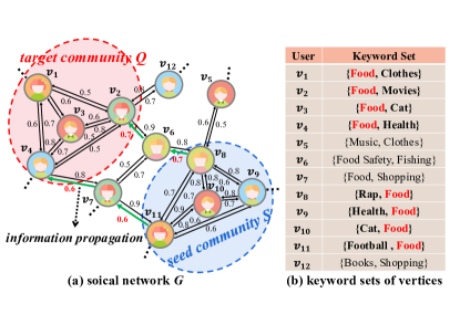
Figure 1. An RICS example over social network $G$.

Example 0.

(Online Advertising and Marketing Over Social Networks) In social networks (e.g., Twitter), a sales manager wants to ensure the optimal advertisement dissemination of some products to a targeted group of users through social networks. Figure 1(a) shows an example of social network $G$, where each user vertex $v_{i}$ ($1\leq i\leq 12$) is associated with a set of keywords (indicating the user’s interests, as depicted in Fig. 1(b)). For example, user $v_{3}$ is interested in delicious food and cute cats. In this scenario, the sales manager can specify a group of targeted customers (e.g., $v_{1}\sim v_{4}$) for online advertising and marketing (forming a target community $Q$), and issue an RICS query to identify a seed community, $S$, of users who have the highest impact on the targeted customers in $Q$ (e.g., via tweets/retweets in Twitter). Users in the returned seed community $S$ will be given coupons or discounts to promote the products on social networks, and most importantly, indirectly affect the targeted customers’ purchase decisions.   $\blacksquare$

Example 0.

(Disease Spread Prevention via Contact Networks) In real application of infectious disease prevention, there exists some community of vulnerable people (e.g., senior/minor people) who are either reluctant or unable to take preventive actions such as vaccines, due to religion, age, and/or health reasons. The health department may want to identify a group of people (e.g., relatives, or colleagues) through contact networks (firestone2011importance, ) who are most likely to spread infectious diseases to such a vulnerable community, and persuade them to use preventive means (e.g., COVID-19 vaccine). In this case, the health department can exactly perform an RICS query to obtain a seed community, $S$, of people who have the highest disease spreading possibilities to the targeted vulnerable community $Q$.   $\blacksquare$

The RICS problem has many other real applications such as finding a group of researchers with the highest influence on another target research community in bibliographical networks.

Inspired by the examples above, in this paper, we consider the RICS problem, which obtains a community (called seed community) that contains query keywords (e.g., food and clothing) and has the highest influence on a target user group. The resulting RICS community contains highly influential users to whom we can promote products for online advertising/marketing, or suggest taking vaccines for protecting vulnerable people in contact networks.

Note that, efficient and effective answering of RICS queries is quite challenging. A straightforward method is to enumerate all possible communities (subgraphs), compute the influence score of each community with respect to the target group, and return a community with the highest influence score. However, this approach is not feasible in practice, due to the large number of candidate communities.

To the best of our knowledge, previous works have not considered the influences on a target user group. Therefore, previous techniques cannot work directly on our RICS problem. To address the challenges of our RICS problem, we propose a two-stage RICS query processing framework in this paper, including offline pre-computation and online RICS querying. In particular, we propose effective pruning strategies (w.r.t., query keyword, boundary support, and influence score) to safely filter out invalid candidate seed communities and reduce the RICS problem search space. Furthermore, we design an effective indexing mechanism to integrate our pruning methods seamlessly and develop an efficient algorithm for RICS query processing.

In this paper, we make the following major contributions.

1. We formally define the reverse influential community search (RICS) problem and its variant, relaxed reverse influential community search (R²ICS), on social networks in Section 2.

2. We design an efficient query processing framework for answering RICS queries in Section 3.

3. We propose effective pruning strategies to reduce the RICS problem search space in Section 4.

4. We devise offline pre-computation and indexing mechanisms in Section 5 to facilitate pruning and online RICS algorithms in Section 6.

5. We develop an efficient online R²ICS processing algorithm to retrieve community answers with the relaxed constraints in Section 7.

6. We demonstrate through extensive experiments the effectiveness and efficiency of our RICS/R²ICS query processing algorithms over real/synthetic graphs in Section 8.

2. Problem Definition

This section first gives the data model for social networks with the information propagation in Section 2.1, then provides the definitions of target and seed communities in social networks in Section 2.2, and finally formulate a novel problem of Reverse Influential Community Search (RICS) over social networks in Section 2.3.

2.1. Social Networks

In this subsection, we model social networks by a graph below.

Definition 0.

(Social Network, $G$) A social network $G$ is a connected graph in the form of a triple $(V(G),E(G),\Phi(G))$, where $V(G)$ and $E(G)$ represent the sets of vertices (users) and edges (relationships between users) in the graph $G$, respectively, and $\Phi(G)$ is a mapping function: $V(G)\times V(G)\rightarrow E(G)$. Each vertex $v_{i}\in V(G)$ has a keyword set $v_{i}.L$, and each edge $e_{u,v}\in E(G)$ is associated with an activation probability $P_{u,v}$.

In a social-network graph $G$ (given by Definition 2.1), each user vertex $v_{i}$ contains topic keywords (e.g., user-interested topics like movies and sports) in a set $v_{i}.L$, and each edge $e_{u,v}$ is associated with an activation probability, $P_{u,v}$, which indicates the influence from user $u$ to user $v$ through edge $e_{u,v}$. Here, the activation probability, $P_{u,v}$, can be obtained based on node attributes (e.g., interests, trustworthiness, locations) (min2020topic, ), network topology (e.g., node degree, connectivity) (ali2022leveraging, ; chen2009efficient, ), or machine learning techniques (fang2014topic, ).

Information Propagation Model: In social networks $G$, we consider an information propagation model defined below.

Definition 0.

(Information Propagation Model) Given an acyclic path $Path_{u,v}=u_{1}\to u_{2}\to\cdots\to u_{m}$ between vertices $u$ ($=u_{1}$) and $v$ ($=u_{m}$) in the social network $G$, we define the influence propagation probability, $\mathit{Pr}(Path_{u,v})$, from $u$ to $v$ as:

(1) $$\mathit{Pr}(Path_{u,v})=\prod_{i=1}^{m-1}P_{u_{i},u_{i+1}},$$

where $P_{u_{i},u_{i+1}}$ is the activation probability from vertex $u_{i}$ to vertex $u_{i+1}$.

Following the maximum influence path (MIP) model (chen2010scalable, ), an MIP, $\mathit{MIP}_{u,v}$, is a path from $u$ to $v$ with the highest influence propagation probability (among all paths $Path_{u,v}$), which is:

(2) $$\mathit{MIP}_{u,v}=\mathop{\arg\max}\limits_{\forall Path_{u,v}}\mathit{Pr}(Path_{u,v}).$$

The influence score, $\mathit{inf\_score}_{u,v}$, from vertex $u$ to vertex $v$ in the social network $G$ is given by:

(3) $$\mathit{inf\_score}_{u,v}=Pr(\mathit{MIP}_{u,v}).$$

2.2. Community

In this subsection, we formally define two terms, target and seed community, as well as the influence from a seed community to a target community, which will be used for formulating our RICS problem.

Target Community: A target community is a group of users whom we would like to influence. For example, in the real application of online advertising/marketing, the target community contains the targeted customers to whom we would like to promote some products; for disease prevention, the target community may contain vulnerable people (e.g., senior/minor people) whom we want to protect from infectious diseases.

Formally, we define the target community as follows.

Definition 0.

(Target Community) Given a social network $G$, a center vertex $v_{q}$, a list, $L_{q}$, of query keywords, and the maximum radius $r$, a target community, $Q$, is a connected subgraph of $G$ (denoted as $Q\subseteq G$), such that:

• $v_{q}\in V(Q)$;

• for any vertex $v_{i}\in V(Q)$, we have $dist(v_{q},v_{i})\leq r$, and;

• for any vertex $v_{i}\in V(Q)$, its keyword set $v_{i}.L$ contains at least one query keyword in $L_{q}$ (i.e., $v_{i}.L\cap L_{q}\neq\emptyset$),

where $dist(x,y)$ is the shortest path distance between $x$ and $y$ in $Q$.

Seed Community: In addition to directly influence the target community (e.g., advertising to targeted users in social networks, or protecting vulnerable people in contact networks), we can also find a group of other users in $G$ (for advertising or protecting, resp.) that indirectly and highly influence the target community. Such a group of influential users forms a seed community.

Definition 0.

(Seed Community) Given a social network $G$, a set, $L_{q}$, of query keywords, a center vertex $v_{s}$, an integer parameter $k$, the maximum number, $N$, of community users, and the maximum radius $r$, a seed community, $S$, is a connected subgraph of $G$ (denoted as $S\subseteq G$), such that:

• $v_{s}\in V(S)$;

• $|V(S)|\leq N$;

• $S$ is a $k$-truss (cohen2008trusses, );

• for any vertex $v_{i}\in V(S)$, we have $dist(v_{s},v_{i})\leq r$, and;

• for any vertex $v_{i}\in V(S)$, its keyword set $v_{i}.L$ contains at least one query keyword in $L_{q}$ (i.e., $v_{i}.L\cap L_{q}\neq\emptyset$).

In Definition 2.4, the seed community $S$ follows the $k$-truss structural constraint (cohen2008trusses, ; huang2017attribute, ), that is, two ending vertices of each edge in the community $S$ have at least $(k-2)$ common neighbors (in other words, each edge is contained in at least $(k-2)$ triangles). This $k$-truss requirement indicates the dense structure of the seed community.

The Calculation of the Community-to-Community Influence: We next define the community-level influence, $inf\_score_{S,Q}$, from a seed community $S$ to a target community $Q$ (w.r.t. topic keywords in $L_{q}$) in social networks $G$.

Definition 0.

(Community-to-Community Influence) Given a target community $Q$, a seed community $S$, the community-to-community influence, $\mathit{inf\_score}_{Q,S}$, of seed community $S$ on target community $Q$ is defined as:

(4) $$\mathit{inf\_score}_{S,Q}=\sum_{u\in V(S)}\sum_{v\in V(Q)}\mathit{inf\_score}_{u,v},$$

where $\mathit{inf\_score}_{u,v}$ is the influence of vertex $u$ on vertex $v$ (as given in Equation (3)).

Intuitively, in Definition 2.5, the community-to-community influence $\mathit{inf\_score}_{S,Q}$ (as given in Equation (4)) calculates the summed influence for all user pairs (in other words, collaborative influence from users in seed community $S$ to that in target community $Q$).

2.3. The Problem Definition of Reverse Influential Community Search Over Social Networks

In this subsection, we propose a novel problem, named Reverse Influential Community Search (RICS) over social networks, which retrieves a seed community $S$ with the highest influence on a given target community in a social network $G$.

The RICS Problem Definition: Formally, we have the following RICS problem definition.

Definition 0.

(Reverse Influential Community Search Over Social Networks, RICS) Given a social network $G=(V(G),E(G),\Phi(G))$, a set, $L_{q}$, of query keywords, an integer parameter $k$, the maximum number, $N$, of community users, and a target community $Q$ (with center vertex $v_{q}$, radius $r$, and query keywords in $L_{q}$), the problem of reverse influential community search (RICS) returns a connected subgraph (community), $S$, from the social network $G$, such that:

• $S$ satisfies the constraints of a seed community (as given in Definition 2.4), and;

• the community-to-community influence, $\mathit{inf\_score}_{S,Q}$, is maximized (i.e., $S=\mathop{\arg\max}\limits_{S\subseteq G}\mathit{inf\_score}_{S,Q}$).

Intuitively, the RICS problem retrieves a keyword-aware seed community $S$ that has the highest influence on the target community $Q$. In real applications such as online advertising/marketing, we can issue the RICS query over the social network $G$ and obtain a seed community $S$ of users to whom we can give group buying coupons or discounts to (indirectly) influence the targeted customers in the target community $Q$.

A Variant, R²ICS, of the RICS Problem: In Definition 2.6, our RICS problem will return the maximum influential seed community, where a seed community needs to fulfill some structural requirements (e.g., $k$-truss and radius constraint, as given in Definition 2.4). In this paper, we also consider a variant of the RICS, named Relaxed Reverse Influential Community Search (R²ICS), which obtains a set of communities with the relaxed structural constraints and having the highest influence.

Definition 0.

(Relaxed Reverse Influential Community Search, R²ICS) Given a social network $G=(V(G),E(G),\Phi(G))$, a set, $L_{q}$, of query keywords, the maximum number, $N$, of community users, and a target community $Q$ (with center vertex $v_{q}$, radius $r$, and query keywords in $L_{q}$), the problem of the relaxed reverse influential community search (R²ICS) returns a subgraph, $S$, from the social network, $G$, such that:

• $S$ is a subgraph of $G$ with size $|V(S)|\leq N$,

• for any vertex $v_{i}\in V(S)$, its keyword set $v_{i}.L$ contains at least one query keyword in $L_{q}$ (i.e., $v_{i}.L\cap L_{q}\neq\emptyset$),and;

• the community-to-community influence, $\mathit{inf\_score}_{S,Q}$, is maximized (i.e., $S=\mathop{\arg\max}\limits_{S\subseteq G}\mathit{inf\_score}_{S,Q}$).

Different from retrieving the seed community in the RICS problem (as given in Definition 2.6), the variant, R²ICS, in Definition 2.7 returns a subgraph community $S$ without the structural constraints such as $k$-truss and radius $r$.

Table 1 lists the commonly used notations and their descriptions in this paper.

Table 1. Symbols and Descriptions

Symbol	Description
$G$	a social network
$V(G)$	a set of vertices $v_{i}$
$E(G)$	a set of edges $e(u,v)$
$\Phi(G)$	a mapping function $V(G)\times V(G)\rightarrow E(G)$
$S$ (or $Q$)	a seed community (or target community) in $G$
$L_{q}$	a set of query keywords
$v_{i}.L$	a set of keywords associated with user $v_{i}$
$v_{i}.BV$	a bit vector with the hashed keywords in $v_{i}.L$
$Path_{u,v}$	an acyclic path from user $u$ to user $v$
$Pr(Path_{u,v})$	the propagation probability that user $u$ activates user $v$ through an acyclic path $Path_{u,v}$
$inf\_score_{u,v}$	the influence score of vertex $u$ on vertex $v$
$inf\_score_{S,Q}$	the community-to-community influence of $S$ on $Q$
$r$-$hop(v_{i},G)$	a subgraph in $G$ with $v_{i}$ as the vertex and $r$ as the radius
$r$	the user-specified radius of target and seed communities
$k$	the support parameter in $k$-truss for the seed community
$sup(e_{u,v})$	the support of edge $e_{u,v}$
$\theta$	the influence threshold

3. The RICS Framework

Algorithm 1 presents our framework for efficiently processing the RICS query, which consists of two phases, that is, offline pre-computation and online RICS-computation phases.

During the offline pre-computation phase, we pre-calculate some data from social networks (for effective pruning) and construct an index over the pre-computed data, which can be used for subsequent online RICS processing. Specifically, for each vertex $v_{i}$ in the social network $G$, we first hash its set, $v_{i}.L$, of keywords into a bit vector $v_{i}.BV$ (lines 1-2). We also pre-calculate a distance vector, $v_{i}.Dist$, which stores the shortest path distances from vertex $v_{i}$ to pivots $piv\in S_{piv}$, where $S_{piv}$ is a set of $d$ carefully selected pivot vertices (line 3). Next, we pre-compute the support bounds, boundary influence upper bound, and influence set for $r$-hop subgraphs (centered at vertex $v_{i}$ and with radii $r$ ranging from 1 to $r_{max}$), in order to facilitate the pruning (lines 4-7). Afterward, we construct a tree index $\mathcal{I}$ on the pre-computed data (line 8).

During the online RICS-computation phase, for each user-specified RICS query, we traverse the index $\mathcal{I}$ and apply our proposed pruning strategies (w.r.t. keywords, support, and influence score) to obtain candidate seed communities (lines 9-10). Finally, we calculate the influence scores between candidate seed communities and $Q$ to obtain the best seed community (line 11).

Input: i) a social network $G$, ii) a set, $L_{q}$, of query keywords, iii) the maximum radius, $r$, of each community, iv) an integer parameter, $k$, of the $k$-truss, v) the maximum user number, $N$, for each seed community, vi) the query center vertex $v_{q}$, and vii) a set, $S_{piv}$, of pivots

Output: a seed community, $S$, with the highest influential score

1

// offline pre-computation phase

2 for each $v_{i}\in V(G)$ do

3       hash keywords in $v_{i}.L$ into a bit vector $v_{i}.BV$

4      compute a vector, $v_{i}.Dist$, of distances from $v_{i}$ to all pivots $piv\in S_{piv}$

5      for $r=1$ to $r_{max}$ do

6             extract $r$-hop subgraph $r$-$hop(v_{i},G)$

7            compute the upper bound of support $ub\_sup(.)$ in $r$-$hop(v_{i},G)$

8            compute the upper bound of boundary influence $ub\_bound\_inf_{r}(.)$ in $r$-$hop(v_{i},G)$

9      

10build a tree index $\mathcal{I}$ over graph $G$ with pre-computed data as aggregates

// online RICS-computation phase

11 for each RICS query do

12      

13      traverse the tree index $\mathcal{I}$ by applying keyword, support, and influence score pruning strategies to retrieve candidate seed communities

14      calculate the influence scores of candidate seed communities and return the one with the highest influential score

Algorithm 1 The RICS Processing Framework

4. Pruning strategies

In this section, we present effective pruning strategies that reduce the problem search space during the online RICS-computation phase (lines 9-11 of Algorithm 1).

4.1. Keyword Pruning

According to Definitions 2.3 and 2.4, each vertex in the target/seed community $Q$ or $S$ must contain at least one keyword from the query keyword set $L_{q}$. Therefore, our keyword pruning method can filter out those candidate subgraphs that do not meet this criterion.

Lemma 4.1.

(Keyword Pruning) Given a set, $L_{q}$, of query keywords and a candidate subgraph (community) $S$, any vertex $v_{i}\in V(S)$ can be safely pruned from $S$, if it holds that: $v_{i}.L\cap L_{q}=\emptyset$, where $v_{i}.L$ is the keyword set associated with vertex $v_{i}$.

Proof.

If $v_{i}.L\cap L_{q}=\emptyset$ holds for any user vertex $v_{i}$ in a candidate community $S$, it indicates that user $v_{i}$ is not interested in any keyword in the query keyword set $L_{q}$. Thus, user vertex $v_{i}$ does not satisfy the keyword constraint in Definition 2.4, and vertex $v_{i}$ can be safely pruned from $S$, which completes the proof.   $\square$ ∎

4.2. Support Pruning

From Definition 2.4, the seed community $S$ needs to be a k-truss (cohen2008trusses, ). Denote the support, $sup(e_{u,v})$ of an edge $e_{u,v}$ as the number of triangles containing $e_{u,v}$. Each edge $e_{u,v}$ in the seed community $S$, is required to have its support $sup(e_{u,v})$ greater than or equal to $(k-2)$. If we can obtain an upper bound, $ub\_sup(e_{u,v})$, of the support for each edge in the candidate seed community $S$, then we can employ the following lemma to eliminate candidate seed communities with low support.

Lemma 4.2.

(Support Pruning) Given a candidate seed community $S$ and a positive integer $k$ $(>2)$, an edge $e_{u,v}$ in $S$ can be discarded safely from $S$, if it holds that $ub\_sup(e_{u,v})<k-2$, where $ub\_sup(e_{u,v})$ is an upper bound of the edge support $sup(e_{u,v})$.

Proof.

In the definition of the $k$-truss (cohen2008trusses, ), the support value, $sup(e_{u,v})$, of the edge $e_{u,v}$ is determined by the number of triangles that contain edge $e_{u,v}$. In a $k$-truss, each edge must be reinforced by at least $(k-2)$ such triangle structures. Since we have the conditions that $ub\_sup(e_{u,v})<k-2$ (lemma assumption) and $sup(e_{u,v})\leq ub\_sup(e_{u,v})$ (support upper bound property), by the inequality transition, we have $sup(e_{u,v})<k-2$. Therefore, based on Definition 2.4, the $k$-truss seed community $S$ cannot include the edge $e_{u,v}$ due to its low support (i.e., $<k-2$). We thus can safely rule out edge $e_{u,v}$ from $S$, which completes the proof.   $\square$ ∎

4.3. Influence Score Pruning

In this subsection, we provide an effective pruning method to filter out candidate seed communities with low influence scores.

Since the exact calculation of the influence score between two communities (given by Equation (4)) is very time-consuming, we can take the maximum influence from candidate seed communities that we have seen as an influence score upper bound (denoted as an influence threshold $\theta$). This way, we can apply the influence score pruning in the lemma below to eliminate those seed communities with low influences.

Lemma 4.3.

(Influence Score Pruning) Let an influence threshold $\theta$ be the maximum influence from candidate seed communities we have obtained so far to the target community $Q$. Any candidate seed community $S$ can be safely pruned, if it holds that $ub\_inf\_score_{S,Q}<\theta$, where $ub\_inf\_score_{S,Q}$ is an upper bound of the influence score $inf\_score_{S,Q}$ (given by Equation (4)).

Proof.

Since $ub\_inf\_score_{S,Q}$ is an upper bound of the influence score $inf\_score_{S,Q}$, we have $inf\_score_{S,Q}\leq ub\_inf\_score_{S,Q}$. Due to the lemma assumption that $ub\_inf\_score_{S,Q}<\theta$, by the inequality transition, it holds that $inf\_score_{S,Q}<\theta$, which indicates that the candidate community $S$ has lower influence on $Q$, compared with some communities we have obtained so far (i.e., with influence $\theta$), and $S$ cannot be our RICS answer. Therefore, we can safely prune candidate seed community $S$, which completes the proof.  $\square$ ∎

5. Offline pre-computation

In this section, we discuss how to offline pre-compute data over social networks, and construct a tree index $\mathcal{I}$ on pre-computed data (lines 1-8 of Algorithm 1).

Input: i) a social network $G$; ii) the maximum radius, $r_{max}$, of each community, and; iii) a set, $S_{piv}$, of $d$ pivots

Output: pre-computed auxiliary data $v_{i}.Aux$ for each vertex $v_{i}$

1

2for each $v_{i}\in V(G)$ do

       // the keyword bit vector

3      

4      hash keywords in $v_{i}.L$ into a bit vector $v_{i}.BV_{0}$

5      $v_{i}.Aux=\{v_{i}.BV_{0}\}$

      // the distance vector to pivots

6      

7      compute a vector, $v_{i}.Dist$, of distances from vertex $v_{i}$ to $d$ pivots in $S_{piv}$

8      add $v_{i}.Dist$ to $v_{i}.Aux$

      // edge support upper bounds

9      

10      for each $e_{u,v}\in E(r_{max}$-$hop(v_{i},G))$ do

11             compute on edge support upper bound $ub\_sup(e_{u,v})$

12      

13

14for each $v_{i}\in V(G)$ do

15      

16      for $r=1$ to $r_{max}$ do

17            

18            $v_{i}.BV_{r}=\bigvee_{\forall{v_{l}\in{r\text{-}hop(v_{i},G)}}}v_{l}.BV$

19            $v_{i}.ub\_sup_{r}=\max_{\forall e_{u,v}\in E(r\text{-}hop(v_{i},G))}ub\_sup(e_{u,v})$

20            $v_{i}.ub\_bound\_inf_{r}=max\{{\sf{collapse\_calculate}}(r\text{-}hop(v_{i},G))\}$

21            add $v_{i}.BV_{r}$ , $v_{i}.ub\_sup_{r}$ and $v_{i}.ub\_bound\_inf_{r}$ to $v_{i}.Aux$

22      

return $v_{i}.Aux$

Algorithm 2 Offline Pre-Computation

5.1. Offline Pre-Computed Data

In order to facilitate online RICS computation, we first conduct offline pre-computations on the social network $G$ in Algorithm 2, which can obtain aggregated information about candidate seed communities (later used for pruning strategies to reduce the online search cost). Specifically, for each vertex $v_{i}$, we hash a set, $v_{i}.L$, of its keywords into a bit vector $v_{i}.BV_{0}$ of size $B$, and initialize a pre-computed set, $v_{i}.Aux$, of auxiliary data with $v_{i}.BV_{0}$ (lines 1-3). Then, we compute the distances from $v_{i}$ to $d$ pivots in $S_{piv}$, forming a distance vector $v_{i}.Dist$ of size $d$, and add $v_{i}.Dist$ to $v_{i}.Aux$ (lines 4-5). Next, we compute a support upper bound, $ub\_sup(e_{u,v})$, for each edge $e_{u,v}$ in a subgraph, $r_{max}\text{-}hop(v_{i},G)$, centered at vertex $v_{i}$ and with radius $r_{max}$ (lines 6-7). Then, for each vertex $v_{i}$ and possible radius $r\in[1,r_{max}]$, we pre-compute a keyword bit vector (lines 8-10), an edge support upper bound (line 11), and an upper bound, $v_{i}.ub\_bound\_inf_{r}$, of boundary influence scores (line 12) for $r\text{-}hop(v_{i},G)$ subgraph. Finally, we add these pre-computed aggregated information to $v_{i}.Aux$ in the following format: $\{v_{i}.BV_{0},v_{i}.Dist,v_{i}.BV_{r},v_{i}.ub\_sup_{r},v_{i}.ub\_bound\_inf_{r}\}$ (line 13).

To summarize, $v_{i}.Aux$ contains the following information:

• a bit vector, $v_{i}.BV_{0}$, of size $B$, which is obtained by using a hashing function $f(l)$ to hash each keyword $l\in v_{i}.L$ to an integer between $[0,B-1]$ and set the $f(l)$-th bit position to 1 (i.e., $v_{i}.BV_{0}[f(l)]=1$);

• a distance vector, $v_{i}.Dist$, of size $d$, which is obtained by computing the shortest path distances, $dist(v_{i},piv)$, from $v_{i}$ to $d$ pivots $piv_{j}\in S_{piv}$; (i.e., $v_{i}.Dist[j]=dist(v_{i},piv_{j})$ for $0\leq j<d$);

• a bit vector, $v_{i}.BV_{r}$ (for $1\leq r\leq r_{max}$), which is obtained by hashing each keyword in keyword set $v_{l}.L$ of a vertex $v_{l}$ in the subgraph $r\text{-}hop(v_{i},G)$ into a position in the bit vector (i.e., $v_{i}.BV_{r}=\bigvee_{\forall{v_{l}\in r\text{-}hop(v_{i},G)}}v_{l}.BV$);

• a support upper bound, $v_{i}.ub\_sup_{r}$, which is obtained by taking the maximum of all support bounds $ub\_sup(e_{u,v})$ for edges $e_{u,v}$ in the subgraph $r\text{-}hop(v_{i},G)$ (i.e., $v_{i}.ub\_sup_{r}=\max_{\forall e_{u,v}\in E(r\text{-}hop(v_{i},G)))}ub\_sup(e_{u,v})$), and;

• an upper bound, $v_{i}.ub\_bound\_inf_{r}$, of boundary influence scores, which is obtained by computing the virtual collapse of a subgraph $r\text{-}hop(v_{i},G)$ discussed below (i.e., $v_{i}.ub\_bound\_inf_{r}=max\{{\sf{collapse\_calculate}}(r\text{-}hop(v_{i},G))\}$), where function collapse_calculate($\cdot$) returns a set, $v_{i}.BIS$, of influence scores through boundary vertices.

Figure 2. An example of seed community virtual collapse operation. The blue arrows represent the information propagation. $v_{c}$ represents a virtual super vertex after the community has collapsed. The red vertices represent the boundary vertices.

Discussions on How to Implement $\sf collapse\_calculate(\cdot)$: Collapse calculations are divided into target collapse and seed collapse. The difference between the two collapses is that the information propagation is in different directions. As shown in Figure 2, a seed community consisting of $v_{1}$, $v_{2}$, $v_{3}$, and $v_{4}$ sends influence to the $1$-hop boundary vertices (i.e., $v_{5}$, $v_{6}$, $v_{7}$, and $v_{8}$). According to Equation (3) and (4), we aggregate the influence of seed communities towards their external boundary vertices. For a virtual collapsed vertex $v_{c}$ of a seed community $S$, through any $1$-hop subgraph boundary vertex $v_{i}$, we have $\mathit{inf\_score}_{v_{c},v_{i}}=\sum_{v\in V(S)}\mathit{inf\_score}_{v,v_{i}}$. Finally, we store the set of boundary influence scores $v_{i}.BIS$ in the center vertex $v_{i}$ of the community.

Complexity Analysis: As shown in Algorithm 2, for each vertex $v_{i}\in V(G)$ in the first loop, the time complexity of computing a keyword bit vector $v_{i}.BV$ is given by $O(|L|)$ (lines 2-3). And the time complexity of computing a distance vector $v_{i}.Dist$ is given by $O((|V(G)|+|E(G)|)\cdot log|V(G)|)$ (lines 4-5). Let $avg\_deg$ denote the average number of vertex degrees. Since there are $avg\_deg^{r_{max}}$ edges in $r_{max}\text{-}hop(v_{i},G)$ and the cost of the support upper bound computation is a constant (counting the common neighbors), so the time cost of obtaining all edge support upper bounds is $O(avg\_deg^{r_{max}})$ (lines 6-7). Thus, the complexity of the first loop (lines 1-7) is given by $O(|V(G)|\cdot(|L|+(|V(G)|+|E(G)|)\cdot log|V(G)|+avg\_deg^{r_{max}}))$.

In the second loop, for each $v_{i}\in V(G)$, there are $avg\_deg^{r-1}$ vertices in the $r\text{-}hop(v_{i},G)$ w.r.t. $r$. Then, for each $r\in[1,r_{max}]$, the time complexity of computing $v_{i}.BV_{r}$ and $v_{i}.ub\_sup_{r}$ is given by $O(B\cdot avg\_deg^{r-1})$ and $O(avg\_deg^{r-1})$, respectively (lines 10-11). As described in Section 5.1, the time complexity of $\sf collapse\_calculate(\cdot)$ is $O((avg\_deg^{r}+avg\_deg^{r-1})\cdot log(avg\_deg^{r-1}))$, and so, the time complexity of $v_{i}.ub\_bound\_inf_{r}$ is given by $O(n\cdot(avg\_deg^{r}+avg\_deg^{r-1})\cdot log(avg\_deg^{r-1}))$. Therefore, the time cost of the second loop (lines 8-13) is $O(|V(G)|\cdot r_{max}\cdot(B\cdot avg\_deg^{r-1}+avg\_deg^{r-1}+n\cdot(avg\_deg^{r}+avg\_deg^{r-1})\cdot log(avg\_deg^{r-1})))$.

In summary, the total time complexity of the total offline pre-computation is given by $O(|V(G)|\cdot(|L|+(|V(G)|+|E(G)|)\cdot log|V(G)|+avg\_deg^{r_{max}}+r_{max}\cdot(B\cdot avg\_deg^{r-1}+avg\_deg^{r-1}+n\cdot(avg\_deg^{r}+avg\_deg^{r-1})\cdot log(avg\_deg^{r-1}))))$.

5.2. Indexing Mechanism

In this subsection, we show the details of offline construction of a tree index $\mathcal{I}$ on a social network $G$ to support online RICS query processing.

The Data Structure of Index $\mathcal{I}$: We will build a tree index $\mathcal{I}$ on the social network $G$, where each index node, $\mathcal{N}$ includes multiple entries $\mathcal{N}_{i}$, each corresponding to a subgraph of $G$. Specifically, the tree index $\mathcal{I}$ contains two types of nodes, leaf and non-leaf nodes.

Leaf Nodes: Each leaf node $\mathcal{N}$ contains multiple vertices $v_{i}$ in the corresponding subgraph. The community subgraph centered at $v_{i}$ is denoted by $r\text{-}hop(v_{i},G)$. Moreover, each vertex $v_{i}$ is associated with the following pre-computed data in $v_{i}.Aux$ (some of them are w.r.t. each possible radius $r\in[1,r_{max}]$):

• a keyword bit vector $v_{i}.BV_{r}$;

• a distance vector $v_{i}.Dist$;

• a support upper bound $v_{i}.ub\_sup_{r}$, and;

• a boundary influence upper bound $v_{i}.ub\_bound\_inf_{r}$.

Non-Leaf Nodes: Each non-leaf node $\mathcal{N}$ has multiple index entries, $\mathcal{N}_{i}$, each of which is associated with the following aggregates (w.r.t. each possible radius $r\in[1,r_{max}]$):

• a pointer to a child node $\mathcal{N}_{i}.ptr$;

• an aggregated keyword bit vector $\mathcal{N}_{i}.BV_{r}=\bigvee_{\forall v_{l}\in\mathcal{N}_{i}}v_{l}.BV_{r}$;

• the distance lower bound vector $\mathcal{N}_{i}.lb\_Dist$ (i.e., $N_{i}.lb\_Dist[j]=\min_{\forall v_{l}\in\mathcal{N}_{i}}v_{l}.Dist[j]$, for $1\leq j\leq d$);

• the distance upper bound vector $\mathcal{N}_{i}.ub\_Dist$ (i.e., $N_{i}.ub\_Dist[j]=\max_{\forall v_{l}\in\mathcal{N}_{i}}v_{l}.Dist[j]$, for $1\leq j\leq d$);

• the maximum support upper bound $\mathcal{N}_{i}.ub\_sup_{r}=\\ \max_{\forall v_{l}\in\mathcal{N}_{i}}v_{l}.ub\_sup_{r}$, and;

• the maximum boundary influence upper bound $\mathcal{N}_{i}.ub\_bound\_inf_{r}=\max_{\forall v_{l}\in\mathcal{N}_{i}}v_{l}.ub\_bound\_inf_{r}$.

Index Construction: To construct the tree index $\mathcal{I}$, we will utilize cost models to first partition the graph into (disjoint) subgraphs of similar sizes to form initial leaf nodes, and then recursively group subgraphs (or nodes) into non-leaf nodes on a higher level, until one final root of the tree is obtained.

Cost Model for the Graph Partitioning: Specifically, we use METIS (karypis1998fast, ) for graph partitioning, guided by our proposed cost model. Our goal of designing a cost model for the graph partitioning is to reduce the number of cases that candidate communities are across subgraph partitions (or leaf nodes), and in turn achieve low query cost.

Assume that a graph partitioning strategy, $\mathcal{P}$, divides the graph into $m$ subgraph partitions $P_{1}$, $P_{2}$, …, and $P_{m}$. We can obtain the number, $Cross\_Par\_Size(\mathcal{P})$, of cross-partition vertices for candidate communities as follows.

$$Cross\_Par\_Size(\mathcal{P})$$

$$= \sum_{j=1}^{m}\sum_{\forall v_{i}\in P_{j}}|V(r_{max}\text{-}hop(v_{i},G)-P_{j})|$$

Since we would like to have the subgraph partitions of similar sizes, we also incorporate the maximum size difference of the resulting partitions in $\mathcal{P}$, and have the following target cost model, $CM(\mathcal{P})$.

(6) $$CM(\mathcal{P})=\mathop{\arg\min_{\mathcal{P}}}(Cross\_Par\_Size(\mathcal{P})+(|\mathcal{P}_{max}|-|\mathcal{P}_{min}|)),$$

where $|\mathcal{P}_{max}|$ and $|\mathcal{P}_{min}|$ represent the numbers of users in the largest and smallest partitions in $\mathcal{P}$, respectively.

Intuitively, we would like to obtain a graph partitioning strategy $\mathcal{P}$ that minimizes our cost model $CM(\mathcal{P})$ (i.e., with low cross-partition search costs and of similar partition sizes, as given in Equation (6)).

Cost-Model-Guided Graph Partitioning for Obtaining Index Nodes: In Algorithm 3, we illustrate how to obtain a set, $\mathbb{S}_{p}$, of $m$ graph partitions for creating index nodes, in light of our proposed cost model above. First, we randomly select $m$ initial vertex pivots and form an initial set, $\mathbb{S}_{piv}$ (line 1). Then, we use $\mathbb{S}_{piv}$ to perform the graph clustering and obtain $m$ partitions in $\mathbb{S}_{p}$ (line 2). We invoke $\sf{calculate\_cost}(\mathbb{S}_{p})$ in Algorithm 4 to calculate the cost, $local\_cost$, of the partitioning $\mathbb{S}_{p}$ (i.e., via $CM(\mathbb{S}_{p})$ in Equation (6) of our cost model; line 3).

Input: i) a social network $G$, ii) the number $m$ of center vertices for partitioning, and iii) the maximum number of iterations $iter_{max}$

Output: a set, $\mathbb{S}_{p}$, of $m$ graph partitions for creating index nodes

1

2randomly select $m$ initial vertex pivots and form $\mathbb{S}_{piv}$

3use $\mathbb{S}_{piv}$ clustering to form $m$ partitions $\mathbb{S}_{p}$

4calculate the cost of the partitioning: $local\_cost=\sf{calculate\_cost}(\mathbb{S}_{p})$

5for $iter=1$ to $iter\_max$ do

6      

7      select a random pivot $piv\in\mathbb{S}_{piv}$

8      randomly select a new vertex $piv_{new}$ that satisfies the requirements of $\mathbb{S}_{piv}$

9      $\mathbb{S}_{piv}^{{}^{\prime}}=\mathbb{S}_{piv}-\{piv\}+\{piv_{new}\}$

10      use $\mathbb{S}_{piv}^{{}^{\prime}}$ clustering to form $m$ partitions $\mathbb{S}_{p}^{{}^{\prime}}$

11      calculate the cost of new partitions: $cost_{new}=\sf{calculate\_cost}(\mathbb{S}_{p}^{{}^{\prime}})$

12      if $cost_{new}<local\_cost$ then

13             $\mathbb{S}_{piv}=\mathbb{S}_{piv}^{{}^{\prime}}$

14            $\mathbb{S}_{p}=\mathbb{S}_{p}^{{}^{\prime}}$

15            $local\_cost=cost_{new}$

16      

17

return $\mathbb{S}_{p}$

Algorithm 3 Cost-Model-Guided Graph Partitioning for Index Nodes

Next, we perform $iter\_max$ iterations to find the best pivot set $\mathbb{S}_{piv}$ and graph partitioning $\mathbb{S}_{p}$ with low cost $local\_cost$ (lines 4-13). In each iteration, we randomly replace one of vertex pivots, $piv$, in $\mathbb{S}_{piv}$ with a new non-pivot vertex $piv_{new}$, forming a new pivot set, $\mathbb{S}_{piv}^{\prime}$ (lines 5-7). This way, we can use $\mathbb{S}_{piv}^{\prime}$ to perform the graph clustering and obtain $m$ new partitions in $\mathbb{S}_{p}^{\prime}$, so that we invoke the function $\sf{calculate\_cost}(\mathbb{S}_{p}^{\prime})$ to calculate a new cost, $cost_{new}$, of partitioning $\mathbb{S}_{p}^{\prime}$ (lines 8-9). Correspondingly, if $cost_{new}$ is less than $local\_cost$, we accept the new partitioning strategy by updating $\mathbb{S}_{piv}$, $\mathbb{S}_{p}$, and $local\_cost$ with $\mathbb{S}_{piv}^{\prime}$, $\mathbb{S}_{p}^{\prime}$, and $cost_{new}$, respectively (lines 10-13). Finally, we return $m$ subgraph partitions, $\mathbb{S}_{p}$, to create $m$ index nodes, respectively (line 14).

Input: a set, $\mathbb{S}_{p}$, of partitions over social network $G$

Output: a cost score, $CM(\mathcal{P})$, for the partitioning in $G$

1 $CM(\mathcal{P})=0$

2for each $P\in\mathbb{S}_{p}$ do

3      

4      for each $v_{i}\in V(P)$ do

5            

6            count the number of vertices that cross the partition $P$’s range: $N\_{cross}=|V(r_{max}\text{-}hop(v_{i},G)-P)|$

7      $Cross\_Par\_Size(P)=\sum_{\forall v_{i}\in P}N\_{cross}$

8      add the value of $Cross\_Par\_Size(P)$ to $CM(\mathcal{P})$

9

10add $|\mathcal{P}_{max}|-|\mathcal{P}_{min}|$ to $CM(\mathcal{P})$

return $CM(\mathcal{P})$

Algorithm 4 calculate_cost($\cdot$) Function

Complexity Analysis: For the tree index $\mathcal{I}$, let $\gamma$ denote the fanout of each non-leaf node $\mathcal{N}$. In $\mathcal{I}$, since the number of leaf nodes is equal to the number of vertices $|V(G)|$, the depth of tree index $\mathcal{I}$ is $\lceil\log_{\gamma}{|V(G)|}\rceil+1$. The time complexity of cost-model-guided graph partitioning for index nodes is given by $O((|V(G)|\cdot m+|V(G)|)\cdot iter\_max)$. On the other hand, the time complexity of recursive tree index construction is $O((\gamma^{dep}-1)/(\gamma-1)\cdot Partitioning)$. Therefore, the time complexity of our tree index construction is given by $O((\gamma^{\lceil\log_{\gamma}{|V(G)|}\rceil+1}-1)/(\gamma-1)\cdot{|V(G)|\cdot(m+1)\cdot iter\_max})$.

6. Online RICS Computation

In this section, we provide our online RICS computation algorithm in Algorithm 5, which traverses our constructed tree index $\mathcal{I}$ and retrieves the RICS community answer that has the highest influence on the target community $Q$, by seamlessly integrating our effective pruning strategies.

Section 6.1 presents effective pruning strategies on the node level of the tree index. Section 6.2 details our proposed online RICS query processing procedure.

6.1. Index Pruning

In this subsection, we present effective pruning methods on the index level, which are used to prune index nodes containing (a group of) community false alarms.

Keyword Pruning for Index Entries: The idea of our keyword pruning over index entries is as follows. If all the $r$-hop subgraphs under an index entry $\mathcal{N}_{i}$ do not contain any keywords in the query keyword set $L_{q}$, then the entire index entry $\mathcal{N}_{i}$ can be safely filtered out.

Below, we provide the index keyword pruning method that uses the aggregated keyword bit vector $\mathcal{N}_{i}.BV_{r}$ stored in $\mathcal{N}_{i}$.

Lemma 6.1.

(Index Keyword Pruning) Given an index entry $\mathcal{N}_{i}$ and a bit vector, $L_{q}.BV$, for the query keyword set $L_{q}$, the index entry $\mathcal{N}_{i}$ can be safely pruned, if it holds that $\mathcal{N}_{i}.BV_{r}\wedge L_{q}.BV=\bm{0}$.

Proof.

If $\mathcal{N}_{i}.BV_{r}\cap L_{q}.BV=\emptyset$ holds, which means that all communities in $\mathcal{N}_{i}$ do not contain any of the keywords in $L_{q}$. According to Definition 2.4, $\mathcal{N}_{i}$ cannot be a candidate seed community, so it can be safely pruned.   $\square$ ∎

Support Pruning for Index Entries: Next, we present the index support pruning method, which utilizes the maximum upper bound support $\mathcal{N}_{i}.ub\_sup_{r}$ of the index entry $\mathcal{N}_{i}$ and the given support $k$ to rule out the entry with low support.

Lemma 6.2.

(Index Support Pruning) Given an index entry $\mathcal{N}_{i}$ and a support parameter $k$, the index entry $\mathcal{N}_{i}$ can be safely pruned, if it holds that $\mathcal{N}_{i}.ub\_sup_{r}<k$, where $\mathcal{N}_{i}.ub\_sup_{r}$ is the maximum support upper bound for all $r$-hop subgraphs under $\mathcal{N}_{i}$.

Proof.

$\mathcal{N}_{i}.ub\_sup_{r}$ is the maximum support upper bound in all $r$-hop subgraphs under index entry $\mathcal{N}_{i}$. If $\mathcal{N}_{i}.ub\_sup_{r}<k$ holds, then all support upper bounds of $r$-hop subgraphs under $\mathcal{N}_{i}$ are less than $k$. By the inequality transition, all the supports of $r$-hop subgraphs under entry $\mathcal{N}_{i}$ are thus less than $k$. Based on Definition 2.4, all $r$-hop subgraphs under $\mathcal{N}_{i}$ cannot be a candidate seed community. Therefore, index entry $\mathcal{N}_{i}$ can be safely pruned, which completes the proof of this lemma.   $\square$

∎

6.2. The RICS Algorithm

In this subsection, we illustrate our online RICS processing algorithm by traversing the tree index $\mathcal{I}$ in Algorithm 5.

Input: i) a social network $G$, ii) a set, $L_{q}$, of query keywords, iii) the maximum radius, $r$, of each community, iv) an integer parameter, $k$, of the truss for each seed community, v) an integer parameter, $N$, of the maximum number of users for each seed community, vi) the query center vertex, $v_{q}$, and vii) the index $\mathcal{I}$

Output: a seed community, $S$, with the highest influential score

1

// initialization

2

3hash all keywords in the query keyword set $L_{q}$ into a query bit vector $L_{q}.BV$

4obtain the target community $Q=r\text{-}hop(v_{q},G)$

5$S=dummy,M=\emptyset,max\_inf\_so\_far=0$

// index traversal

6

7initialize a minimum heap $\mathcal{H}$ accepting index entries in the form $(\mathcal{N},key)$

8insert all entries $\mathcal{N}$ in the root of index $\mathcal{I}$ into heap $\mathcal{H}$

9while $\mathcal{H}$ is not empty do

10      

11      $(\mathcal{N},key)=\mathcal{H}.pop()$

12      if $max\_inf\_so\_far\geq max\_inf\_ub(\mathcal{H})$ then

13             terminal the loop

14      

15      if $\mathcal{N}$ is a leaf node then

16             for each vertex $v_{i}\in\mathcal{N}$ do

17                   obtain the candidate community $C=\mathcal{N}.r\text{-}hop(v_{i},G)$

18                  if $C$ cannot be pruned by Lemma 4.1, 4.2, or 4.3 then

19                         if $C$ is closer to $Q$ than $S$ and is larger than $S$ then

20                              

21                              compute the influence score $inf\_score_{C,Q}=\sf{calculate\_influence}$$(C,Q)$

22                              if $inf\_score_{C,Q}>max\_inf\_so\_far$ then

23                                    

24                                    if $|V(C)|\leq N$ then

25                                          

26                                          $max\_inf\_so\_far$$=$$inf\_score_{C,Q}$

27                                          $S=C$

28                                    else

29                                           update $C$ to be the $k$-truss subgraph of $C$ of size $N$ with maximal influence score $inf\_score_{C,Q}$

30                                          if $inf\_score_{C,Q}>max\_inf\_so\_far$ then

31                                                

32                                                $max\_inf\_so\_far$$=$$inf\_score_{C,Q}$

33                                                $S=C$

34                                          

35                                    

36                              

37                        else

38                               if $v_{i}.ub\_inf\_score_{r}>max\_inf\_so\_far$ then

39                                     add $C$ to $M$

40                              

41                        

42                  

43            

44      else

             // $\mathcal{N}$ is a non-leaf node

45             for each entry $\mathcal{N}_{i}\in\mathcal{N}$ do

46                  

47                  if $\mathcal{N}_{i}$ cannot be pruned by Lemma 6.1 or 6.2 then

48                        

49                        insert $(\mathcal{N}_{i},key)$ into heap $\mathcal{H}$

50                  

51            

52      

53

// refinement of candidate communities

54

55update $M$ by sorting on influence score upper bounds

56for each candidate community $C\in M$ do

57      

58      if $max\_inf\_so\_far>C.ub\_inf\_score_{r}$ then

59            

60            terminal the loop

61      

62      select no more than $N$ vertices to form a community $C^{\prime}$ from $C$

63      compute the influence score $inf\_score_{C^{\prime},Q}={\sf calculate\_influence(C^{\prime},Q)}$

64      if $inf\_score_{C^{\prime},Q}>max\_inf\_so\_far$ then

65            

66            $max\_inf\_so\_far=inf\_score_{C^{\prime},Q}$

67            $S=C^{\prime}$

68      

return $S$

Algorithm 5 Online RICS Processing

Initialization: First, our RICS algorithm obtains a query bit vector $L_{q}.BV$ by hashing all keywords from the query keyword set $L_{q}$ (line 1). Then, according to the given query center vertex $v_{q}$, the algorithm determines the target community $Q$ (line 2). After that, we initialize an initially dummy community $S$ to store the best seed community we have searched so far. Moreover, we maintain an initially empty set, $M$, which keeps a set of potential candidate communities for delayed refinement. We also set a variable, $max\_inf\_so\_far$, to $0$, which indicates the highest influence score we have encountered so far for the early termination of the index traversal (line 3).

Index Traversal: To facilitate the index traversal, we maintain a minimum heap $\mathcal{H}$, which accepts heap entries in the form $(\mathcal{N},key)$, where $\mathcal{N}$ is an index node, and $key$ is the minimum lower bound of the distances from vertices under node $\mathcal{N}$ to query vertex $v_{q}$ (line 4). To start the index traversal, we insert all entries in the root of index $\mathcal{I}$ into heap $\mathcal{H}$ (line 5). Then, we traverse the index by accessing entries from $\mathcal{H}$ in ascending order of distance lower bounds (intuitively, communities closer to $v_{q}$ will have higher influences on $Q$; lines 6-31).

Specifically, each time we pop out an index entry $(\mathcal{N},key)$ with the minimum key from heap $\mathcal{H}$ (line 7). If $max\_inf\_so\_far\geq max\_inf\_ub(\mathcal{H})$ holds, which indicates that all the candidate communities in the remaining entries of $\mathcal{H}$ cannot have higher influences than the communities we have already obtained, then we can terminate the index traversal (lines 8-9); otherwise, we will check the entries in the node $\mathcal{N}$.

When $\mathcal{N}$ is a leaf node, for each vertex $v_{i}\in\mathcal{N}$, we first obtain its candidate community $C=r\text{-}hop(v_{i},G)$ centered at $v_{i}$ (line 12). Then, for the candidate community $C$, we apply the Keyword Pruning (Lemma 4.1), Support Pruning (Lemma 4.2), and Influence Score Pruning (Lemma 4.3) (lines 13). If $C$ cannot be ruled out by these three pruning methods, we will check whether $C$ will be larger and closer to $Q$ than $S$ (line 14). This is because, intuitively, such candidate communities have more influence on $Q$. After that, we calculate the exact influence, $inf\_score_{C,Q}$, from $C$ to target community $Q$, by invoking the function calculate_influence$(C,Q)$ (line 15). If the influence $inf\_score_{C,Q}$ is higher than the highest influence score, $max\_inf\_so\_far$, and the seed community $C$ is of small scale (i.e., $\leq N$), we will update the current answer $S$ and its influence score $max\_inf\_so\_far$ (lines 16-19). If the seed community $C$ is of large scale (i.e., $>N$), we will update $C$ to be the $k$-truss subgraph of $C$ of size $N$ with the largest influence score $inf\_score_{C,Q}$ of all $k$-truss subgraphs (lines 20-21). Then, like the small scale, if the influence $inf\_score_{C,Q}$ is higher than the highest influence score, $max\_inf\_so\_far$, we will update the current answer $S$ and the highest influence score $max\_inf\_so\_far$ (lines 22-24). On the other hand, although $C$ is not better than $S$ in terms of position and size, it also has the potential to have the highest influence on $Q$. If its influence score upper bound (for any subgraphs of size $N$) is greater than the highest influence, we will add $C$ to the candidate set $M$ for later refinement (lines 25-27).

When $\mathcal{N}$ is a non-leaf node, we will consider each child node $\mathcal{N}_{i}\in\mathcal{N}$ (lines 28-29). If entry $\mathcal{N}_{i}$ cannot be pruned by Index Keyword Pruning (Lemma 6.1) and Index Support Pruning (Lemma 6.2), we insert the entry $(\mathcal{N}_{i},key)$ into heap $\mathcal{H}$ for further investigation (lines 30-31).

When either the heap $\mathcal{H}$ is empty (line 6) or the remaining index entries in $\mathcal{H}$ cannot contain candidate communities (line 8), we will terminate the index traversal.

Refinement of Candidate Communities: After the index traversal, we update $M$ by sorting candidate communities in descending order of influence score upper bounds (line 32). Then, for each candidate community $C$ in the list $M$, if it holds that $max\_inf\_so\_far>C.ub\_inf\_score_{r}$, then we can stop checking the remaining candidates in $M$ (as all candidates in $M$ have influence upper bounds less than highest influence so far; lines 34-35). Next, we compute a seed community $C^{\prime}$ of size no more than $N$ from $C$ (i.e., $C^{\prime}\subset C$) with the highest influence, $inf\_score_{C^{\prime},Q}$, on target community $Q$ (lines 36-37). If it holds that $inf\_score_{C^{\prime},Q}>max\_inf\_so\_far$, then we need to update the RICS answer $S$ with $C^{\prime}$ (replacing $max\_inf\_so\_far$ with $inf\_score_{C^{\prime},Q}$ as well; lines 38-40). Finally, after refining $M$, we return the seed community $S$ as our RICS answer (line 41).

Discussions on the Computation of $\sf{calculate\_influence}(C,Q)$: To exactly calculate the community-to-community influence score (via Equation (3) and (4)), we need to obtain the influence of each user in the seed community $C$ on the target community $Q$, the whole process is similar to the single-source shortest path algorithm. For each point $v_{c}$ in C, we first visit its 1-hop neighbors $v_{b}$ and the influence score $inf\_score_{vc,vb}=P_{vc,vb}$. Then, each time, we extend 1-hop neighbors $v_{new}$ forward and compute the current influence score $inf\_score_{vc,v_{new}}=\max_{\forall{v_{i}\in v_{new}}}(inf\_score_{v_{new},v_{i}}\cdot P_{v_{new},v_{i}})$, of $v_{c}$, until we get the maximum influence score on all node of $Q$.

Discussions on the Online Computation of Influence Upper Bound $v_{i}.ub\_inf\_score_{r}$: Since we get the upper bound of boundary influence score, $v_{i}.ub\_bound\_inf_{r}$, of $\sf{collapse\_calculate}$ data for a subgraph $r\text{-}hop(v_{i},G)$, and for a target community, $Q$, with query center vertex, $v_{q}$, we can get the distance lower bound $lb\_dist(v_{i},v_{q})=\min([|v_{i}.Dist[j]-v_{q}.Dist[j]|]$, for $1\leq j\leq d)$ between $v_{i}$ and $v_{q}$ by triangle inequality (Plaisted84, ). Then, we can get the upper bound of influence score, $v_{i}.ub\_inf\_score_{r}=v_{i}.ub\_bound\_inf_{r}\cdot|V(Q)|\cdot\max(P)^{lb\_dist(v_{i},v_{q})-2\cdot r}$, where $\max(P)$ denotes the maximum neighbor activation probability in $G$.

Complexity Analysis: Let $\overline{n_{r}}$ be the average number of users in the target community $Q$. The cost of obtaining $L_{q}.BV$ and $Q$ takes $O(\overline{n_{r}})$. Let $PP_{j}$ be the pruning power (i.e., the percentage of node entries that can be pruned) on the $j$-th level of the tree index $\mathcal{I}$, where $0\leq j\leq h$ and $h$ is the height of the tree. Denote $f$ as the average fanout of nodes in index $\mathcal{I}$. For the index traversal, the number of visited nodes is given by $O(\sum_{j=1}^{h}f_{h-j+1}\cdot(1-PP_{j}))$. We label a subgraph $r\text{-}hop(v_{i},G)$ as $g$. Each time, the function of $\sf{calculate\_influence}$ need $O((V|g|+E|g|)\cdot\overline{n_{r}})$. Let $\overline{n_{d}}$ be the average number of iterations updated due to the closest distance. Then, the updating $S$ and $max\_inf\_so\_far$ takes $O((V|g|+E|G|)\cdot\overline{n_{r}}\cdot\overline{n_{d}})$. And, updating $M$ takes $O(1)$. For the refinement process, let $\overline{n_{m}}$ be the average number of calculate influence in $M$, and the updating $S$ and $max\_inf\_so\_far$ take $O(1)$. Therefore, the total time complexity of Algorithm 5 is given by $O(\sum_{j=1}^{h}f_{h-j+1}\cdot(1-PP_{j})+((V|g|+E|g|)\cdot(\overline{n_{d}}+\overline{n_{m}})+1)\cdot\overline{n_{r}})$.

7. Online Computation for R²ICS

In this section, we design an effective pruning strategy w.r.t. vertex-to-community influence score to reduce the search space of our R²ICS problem, and develop an efficient algorithm for retrieving the R²ICS community answer.

Effective Pruning Strategy w.r.t. Vertex-to-Community Influence Score: In order to R²ICS community answer $S$ in $G$ with the highest influence $inf\_score_{S,Q}$, a straightforward method is to enumerate all the vertex combinations and find a community that meets the requirements, which is however rather inefficient. Instead, we observed that the community-to-community influence score $inf\_score_{S,Q}$ (as given in Eq. (4)) is given by summing up vertex-to-community influences, $inf\_score_{v,Q}$, for all $v\in V(S)$. Based on this observation, our basic idea about the R²ICS algorithm is to retrieve those vertices $v$ with high vertex-to-community influences on $Q$ first and early terminate the search to prune or avoid accessing those low-influence vertices.

Therefore, to enable the pruning of low-influence vertices, we propose an effective vertex-to-community influence score pruning strategy as follows.

Lemma 7.1.

(Vertex-to-Community Influence Score Pruning) Let $min\_inf\_so\_far$ be the minimum vertex-to-community influence from vertices in the best-so-far candidate R²ICS community $S$ of size $N$ to the target community $Q$. Any vertex $v$ can be safely pruned, if it holds that $ub\_inf\_score_{v,Q}<min\_inf\_so\_far$, where $ub\_inf\_score_{v,Q}$ is an upper bound of the influence score $inf\_score_{v,Q}$.

Proof.

Since $ub\_inf\_score_{v,Q}$ is an upper bound of the influence score $inf\_score_{v,Q}$, we have $inf\_score_{v,Q}\geq ub\_inf\_score_{v,Q}$. If $ub\_inf\_score_{v,Q}<min\_inf\_so\_far$ holds, means $inf\_score_{v,Q}<min\_inf\_so\_far$, which indicates that the vertex $v$ has a lower influence on $Q$, compared with some vertices we have obtained so far (i.e., with influence $min\_inf\_so\_far$), and $v$ cannot be our R²ICS answer. Therefore, we can safely prune candidate vertex $v$, which completes the proof. ∎

A Framework for the R²ICS Algorithm: Algorithm 6 illustrates the pseudo code of our R²ICS algorithm over a social network $G$, which consists of initialization, index traversal, and candidate vertex refinement phases. We first initialize the data/variables that will be used in Algorithm 6 (lines 1-3). Then, for each user-specified R²ICS query, we traverse the index $\mathcal{I}$ to obtain candidate vertices, by applying our proposed keyword pruning strategies in Sections 4.1 and 6.1 (lines 4-23). Finally, we refine candidate vertices and return an actual R²ICS community $S$ with the highest influence $inf\_score_{S,Q}$ (lines 24-41).

Initialization: In the initialization phase, the algorithm first hashes all the query keywords in $L_{q}$ into a query keyword bit vector $L_{q}.BV$, and then obtain the target community $Q$ (i.e., $r$-hop subgraph with center vertex $v_{q}$) (lines 1-2). Next, we prepare an initially dummy community $S$ to store the best community we have searched so far, an initially empty set, $v2C\_inf\_set$, to store vertex-to-community influence scores of each vertex in $S$ on $Q$, and an empty candidate vertex set, $V_{cand}$, for later refinement (line 3).

Index Traversal: We utilize a minimum heap $\mathcal{H}$ with heap entries ($\mathcal{N},key$) for the index traversal, where $\mathcal{N}$ is an index node, and $key$ is defined as the lower bound of distances from vertices under node $\mathcal{N}$ to query vertex $v_{q}$ (line 4). To start the index traversal, we insert all entries $\mathcal{N}$ in the root of index $\mathcal{I}$ into heap $\mathcal{H}$ (line 5).

Each time we pop out an index entry $(\mathcal{N},key)$ with the minimum key from heap $\mathcal{H}$ (lines 6-7). When $\mathcal{N}$ is a leaf node, for each vertex $v_{i}\in\mathcal{N}$, we apply the keyword pruning (Lemma 4.1) (lines 8-10). If $v_{i}$ cannot be ruled out by this pruning method, we will decide whether we add $v_{i}$ to $S$ or $V_{cand}$ (lines 11-19). If the candidate community $S$ has not reached its maximum size $N$ and $v_{i}\in\mathcal{N}$ is closer to $v_{q}$ than all vertices in $S$ (i.e., potentially having higher influence on $Q$), we will compute the exact vertex-to-community influence score $inf\_score_{v_{i},Q}$, add vertex $v_{i}$ to $S$, and update set $v2C\_inf\_set$ by adding $inf\_score_{v_{i},Q}$ (lines 11-15); otherwise (i.e., $|V(S)|=N$ or $v_{i}$ is far away from $v_{q}$), we will add vertex $v_{i}$ to the vertex candidate set $V_{cand}$ for later refinement (lines 16-19).

When $\mathcal{N}$ is a non-leaf node, we will consider each child node $\mathcal{N}_{i}\in\mathcal{N}$ (lines 20-21). If $\mathcal{N}_{i}$ cannot be pruned by Lemma 6.1, then we insert entry ($\mathcal{N}_{i},key$) into heap $\mathcal{H}$ for further investigation (lines 22-23).

Candidate Vertex Refinement: Next, we will further check candidate vertices in $V_{cand}$ and see whether any of them can be added to or replace some vertices in $S$ to achieve higher influence. Specifically, we first sort candidate vertices in $V_{cand}$ in descending order of influence score upper bounds, and let an influence threshold, $min\_inf\_so\_far$, be the minimum influence score in $v2C\_inf\_set$ we have searched so far (lines 24-25).

After that, we consider each candidate vertex $v_{i}\in V_{cand}$ in descending order of their influence score upper bounds (line 26). There are two cases below:

• Case 1 (Community $S$ reaches its maximum size $N$): We will use Lemma 7.1 to determine whether to terminate the loop early (lines 27-28). If $v_{i}$ can be pruned via vertex-to-community influence, then all the remaining entries (vertices) in heap $\mathcal{H}$ will have influences below $min\_inf\_so\_far$ and we can terminate the search safely (lines 33-35). If $v_{i}$ cannot be pruned, then we will calculate the exact influence score $inf\_score_{v_{i},Q}$ of $v_{i}$ on $Q$. If $inf\_score_{v_{i},Q}$ is greater than $min\_inf\_so\_far$, we will replace one vertex in $S$ which has the smallest vertex-to-community influence with $v_{i}$ (lines 30-31). Correspondingly, we update $v2C\_inf\_set$, upon the replacement of vertex $v_{i}$ and set $min\_inf\_so\_far$ to the updated minimum value in $v2C\_inf\_set$ (lines 32-33).

• Case 2 (Community $S$ does not reach its maximum size $N$): In this case, $|V(S)|<N$ holds, which indicates that we can still include more vertices for higher influence. Then, we will compute the influence score $inf\_score_{v_{i},Q}$ of $v_{i}$ on $Q$, add $v_{i}$ and $inf\_score_{v_{i},Q}$ to $S$ and $v2C\_inf\_set$, respectively, and update the threshold $min\_inf\_so\_far$ (lines 36-40).

After the refinement, we obtain a community $S$ of up to $N$ vertices with the highest influence, and return $S$ as the R²ICS answer (line 41).

Discussions on the Correctness of the R²ICS Algorithm: Since we only use the keyword pruning during the index traversal phase, we can obtain a best-so-far community $S$ (i.e., $1\leq|V(S)|\leq N$) and a set, $v2C\_inf\_set$, containing all candidate vertices that meet the keyword requirement. Thus, we do not miss any vertices with high influences on $Q$ in this step. In Definition 2.5, the community-to-community influence is given by the summation of vertex-to-community influences. From our R²ICS algorithm in Algorithm 6), we always include in $S$ those vertices $v_{i}$ with the highest vertex-to-community influence $inf\_score_{v_{i},Q}$ (lines 30-33). Thus, the resulting R²ICS community $S$ is guaranteed to achieve the highest community-to-community influence score $inf\_score_{S,Q}$.

Complexity Analysis: As the same Algorithm 5, the initialization and index traversal phase of our R²ICS takes $O(\sum_{j=1}^{h}f_{h-j+1}+(V|g|+E|g|+1)\cdot\overline{n_{r}}\cdot N)$. For refinement, let $GPP$ be the vertex-to-community influence score pruning power (i.e., the percentage of vertices that can be pruned). And, updating $S$, $v2C\_inf\_set$ and $min\_inf\_so\_far$ takes $O(1)$. Therefore, the total time complexity of Algorithm 6 is given by $O(\sum_{j=1}^{h}f_{h-j+1}+((V|g|+E|g|)\cdot(N+|V(G)|\cdot GPP)+1)\cdot\overline{n_{r}})$

Input: i) a set, $L_{q}$, of query keywords, ii) a query center vertex, $v_{q}$, iii) the maximum radius, $r$, of the target community $Q$, iv) the maximum number, $N$, of users in the R²ICS community, and v) the index $\mathcal{I}$ over social networks $G$

Output: an R²ICS community answer $S$

1

// initialization phase

2

3hash all keywords in the query keyword set $L_{q}$ into a query bit vector $L_{q}.BV$

4obtain the target community $Q=r\text{-}hop(v_{q},G)$

5$S=dummy,v2C\_inf\_set=\emptyset,V_{cand}=\emptyset$;

// index traversal phase

6

7initialize a minimum heap $\mathcal{H}$ accepting index entries in the form $(\mathcal{N},key)$

8insert all entries $\mathcal{N}$ in the root of index $\mathcal{I}$ into heap $\mathcal{H}$

9while $\mathcal{H}$ is not empty do

10      

11      $(\mathcal{N},key)=\mathcal{H}.pop()$

12      if $\mathcal{N}$ is a leaf node then

13             for each vertex $v_{i}\in\mathcal{N}$ do

14                  

15                  if  $v_{i}$ cannot be pruned by Lemma 4.1 then

16                        

17                        if $|V(S)|$ ¡ $N$ then

18                               if $v_{i}$ is closer to $v_{q}$ than all vertices $v_{s}\in S$ then

19                                    

20                                    compute the influence score $inf\_score_{v_{i},Q}=\sf{calculate\_influence}$$(v_{i},Q)$

21                                    add $v_{i}$ to $S$

22                                    add $inf\_score_{v_{i},Q}$ to $v2C\_inf\_set$

23                              else

24                                     add $v_{i}$ to $V_{cand}$

25                              

26                        else

27                               add $v_{i}$ to $V_{cand}$

28                        

29                  

30            

31      else

             // $\mathcal{N}$ is a non-leaf node

32             for each entry $\mathcal{N}_{i}\in\mathcal{N}$ do

33                   if $\mathcal{N}_{i}$ cannot be pruned by Lemma 6.1 then

34                         insert $(\mathcal{N}_{i},key)$ into heap $\mathcal{H}$

35                  

36            

37      

38

// candidate vertex refinement phase

39

40sort candidate vertices in $V_{cand}$ in descending order of influence score upper bounds

41$min\_inf\_so\_far=\min(v2C\_inf\_set)$

42for each candidate vertex $v_{i}\in V_{cand}$ do

43      

44      if $|V(S)|=N$ then

45            

46            if $v_{i}$ cannot be pruned by Lemma 7.1 then

47                  

48                  compute the influence score $inf\_score_{v_{i},Q}=\sf{calculate\_influence}$$(v_{i},Q)$

49                  if $inf\_score_{v_{i},Q}>min\_inf\_so\_far$ then

50                        

51                        replace one vertex in $S$ (having the smallest vertex-to-community influence, $min\_inf\_so\_far$, in $v2C\_inf\_set$) with $v_{i}$

52                        update $v2C\_inf\_set$, upon the replacement of vertex $v_{i}$

53                        update $min\_inf\_so\_far=\min(v2C\_inf\_set)$

54                  

55            else

56                   terminate the loop

57            

58      else

59             compute the influence score $inf\_score_{v_{i},Q}=\sf{calculate\_influence}$$(v_{i},Q)$

60            add $v_{i}$ to $S$

61            add $inf\_score_{v_{i},Q}$ to $v2C\_inf\_set$

62            update $min\_inf\_so\_far=\min(v2C\_inf\_set)$

63      

return $S$

Algorithm 6 Online R²ICS Processing

8. Experimental evaluation

8.1. Experimental Settings

We evaluate the performance of the online RICS algorithm (i.e., Algorithm 5) on both real and synthetic graph data sets.

Real-World Graph Data Sets: We use three real-world graphs, Facebook (leskovec2012learning, ), Amazon (yang2012defining, ), and DBLP (zhou2009graph, ), whose statistics are depicted in Table 2. Facebook is a social network, where two users are connected if they are friends. Amazon is an Also Bought network, where two products are connected if they are purchased together. DBLP is a co-authorship network, where two authors are connected if they publish at least one paper together.

Synthetic Graph Data Sets: We construct synthetic social networks by generating small-world graphs $G$ (newman1999renormalization, ). Specifically, we first create a ring of size $|V(G)|$, and then connect $m$ nearest neighbor nodes for each vertex $u$. Next, for each generated edge $e_{u,v}$, we add a new edge $e_{u,w}$ with probability $\mu$ that connects $u$ to a random vertex $w$. Here, we take $m$ = 5 and $\mu$ = 0.251. For each vertex, we randomly generate a keyword set $v_{i}.L$ from the keyword domain $\Sigma$, following $Uniform$, $Gaussian$, and $Zipf$ distributions, to obtain three synthetic graphs, denoted as $Uni$, $Gau$, and $Zipf$, respectively. Next, for each edge $e_{u,v}$ in the generated graphs, we produce a random value within an interval $[0.5,0.6)$ as the edge activation probability $P_{u,v}$.

Table 2. Statistics of the tested real-world graph data sets.

Social Networks	$|V(G)|$	$|E(G)|$
Facebook(leskovec2012learning, )	4,039	88,234
Amazon(yang2012defining, )	334,863	925,872
DBLP(zhou2009graph, )	317,080	1,049,866

Table 3. Parameter settings.

Parameters	Values
support, $k$, of truss structure	3, 4, 5
radius $r$	1, 2, 3
size, $|L_{q}|$, of query keywords set	2, 3, 5, 8, 10
size, $|v_{i}.L|$, of keywords per vertex	1, 2, 3, 4, 5
keyword domain size $|\Sigma|$	10, 20, 50, 80
the number, $d$, of pivots	3, 5, 8, 10
the maximum size, $N$, of seed community	5, 10, 15, 20
the size, $|V(G)|$, of data graph $G$	10K, 25K, 50K, 100K, 250K

Competitors: To our best knowledge, no prior works studied the RICS problem and its variant, R²ICS, by considering the influence of a connected community on a user-specified target community (instead of the entire graph). Therefore, we compare our RICS approach with a straightforward method, called baseline. The baseline method first determines the target community $Q$ based on the given query vertex and then performs Breadth First Search (BFS) from $Q$ in the social network $G$. For each vertex we encounter (during the BFS traversal), baseline obtains its $r$-hop subgraph and checks whether this subgraph satisfies the structure and keyword constraints. Next, we obtain candidate communities $S$ from the $r$-hop subgraph and calculate their influence scores $inf\_score_{S,Q}$. If a candidate community $S$ has an influence score greater than the best score we have seen so far, we will let $S$ be the best-so-far RICS answer. Finally, after all vertices have been traversed, baseline returns the candidate community $S$ we have obtained with the maximum influence on the target community $Q$. Note that, since the time cost of the baseline method is extremely high, we evaluate this method by sampling $0.1\%$ vertices from the data graph $G$ without replacement. Therefore, the total time can be estimated by $\overline{t}\cdot|V(G)|$, where $\overline{t}$ denotes the average time of each sample.

For R²ICS, we compare our approach (R²ICS, Algorithm 6) with R²ICS_WoP and Optimal methods. Here, R²ICS_WoP is our R²ICS approach without the pruning strategy in Section 7, whereas Optimal computes the influence score of each vertex on the target community in the original graph and selects a combination of $N$ vertices with the highest influence score as the query result.

Measure: To evaluate the efficiency of our RICS / R²ICS approaches, we randomly select 50 query nodes from each graph data set, and take the average of the wall clock time over 50 runs, which is the time cost of online retrieving RICS or R²ICS query results via the index (Algorithms 5 and 6).

Figure 3. The RICS performance on real/synthetic graphs.

Parameter Settings: Table 3 depicts parameter settings, where default values are in bold. Each time, we vary the value of one parameter while setting other parameters to their default values. We ran all the experiments on the PC with Intel(R) Core(TM) i9-10900K CPU 3.70GHz and 32 GB memory. All algorithms were implemented in Python and executed with Python 3.8 interpreter.

8.2. Performance Evaluation

The RICS Performance on Real/Synthetic Graphs: Figure 3 illustrates the performance of our RICS approach on both real and synthetic graphs, compared with the baseline method, where all parameters are set by their default values in Table 3, except for the dense Facebook dataset with the maximum seed community size $N$ = 700. Experimental results show that the wall clock time of our RICS approach outperforms baseline by almost three orders of magnitude, which confirms the effectiveness of our proposed pruning strategies and indexing mechanisms and the efficiency of our RICS approach.

To evaluate the robustness of our RICS approach, in subsequent experiments, we will test the effect of each parameter in Table 3 on the query performance over synthetic graphs.

Effect of Truss Support Parameter $k$: Figure LABEL:fig:subfigures(a) shows the RICS query performance for different $k$ values, where $k$ = 3, 4, and 5, and the rest of parameters are set to default values. From this figure, we can find that for larger $k$ values, the query time cost decreases over all three synthetic graphs. This is because larger $k$ leads to fewer candidate communities satisfying the $k$-truss constraints, which in turn incurs lower wall clock time.

Effect of Radius $r$: Figure LABEL:fig:subfigures(b) illustrates the wall clock time of our RICS approach, by varying $r$ from 1 to 3, where other parameters are set to their default values. When the radius $r$ increases, the numbers of vertices included in the target and seed communities also increase, leading to higher filtering and refinement costs. Nevertheless, the wall clock time remains low (i.e., $3.54\sim 17.44$ $sec$) for all the synthetic graphs.

Effect of the Size, $|L_{q}|$, of the Query Keyword Set: Figure LABEL:fig:subfigures(c) presents the RICS query performance, where $|L_{q}|$ = 2, 3, 5, 8, and 10, and other parameters are by default. Intuitively, as $|L_{q}|$ increases, more candidate seed communities satisfy the keyword requirements. Thus, we will have a higher threshold of the influence score, which results in higher pruning power and, in turn, lower time cost, as confirmed by the figure. However, more candidate seed communities require more refinement costs, and wall clock times increase. In summary, the wall clock time remains low for different $|L_{q}|$ values (i.e., $4.86\sim 29.56$ $sec$).

Effect of the Size, $|v_{i}.L|$, of Keywords per vertex: Figure LABEL:fig:subfigures(d) reports the efficiency of our RICS approach, by varying $|v_{i}.L|$ from 1 to 5, where default values are used for other parameters. With the increase of $|v_{i}.L|$, more vertices are likely to be included in candidate seed communities, which leads to a higher influence threshold and higher pruning power (or lower query cost). Meanwhile, larger $|v_{i}.L|$ will incurs higher filtering/refinement costs. Therefore, the two factors mentioned above show that the wall clock time first decreases and then increases for larger $|v_{i}.L|$. The wall clock times with different $|v_{i}.L|$ values are $4.88\sim 13.73$ $sec$.

Effect of Keyword Domain Size $|\Sigma|$: Figure LABEL:fig:subfigures(e) illustrates the RICS query performance with different keyword domain sizes $|\Sigma|$ = 10, 20, 50, and 80, where other parameters are set to default values. From this figure, we can find that, since larger $\Sigma$ will improve the pruning power of keyword pruning, the community computational cost decreases. On the other hand, fewer candidate communities also lead to lower impact thresholds and lower pruning power. Thus, for all three synthetic graphs, the wall clock time decreases and then increases as $\Sigma$ increases. Nevertheless, the wall clock times remain low (i.e., $4.92\sim 30.75$ $sec$).

Effect of the Number, $d$, of Pivots: Figure LABEL:fig:subfigures(f) shows the RICS query performance for various numbers of pivots, where $d$ = 3, 4, 5, 6, and 8, and default values are used for other parameters. When $d$ increases, the distance lower bounds from candidate communities $S$ to target community $Q$ are tighter, which incurs better searching order of candidate communities and achieves higher influence threshold earlier (or lower query costs). However, more pivots will also lead to higher computation costs for distances with lower bounds. Therefore, in the figure, for larger $d$ values, the wall clock time first decreases and then increases. Nonetheless, the wall clock times remain low (i.e., $4.92\sim 9.97$ $sec$).

Effect of the Maximum Size, $N$, of Seed Communities: Figure LABEL:fig:subfigures(g) evaluates the performance of our RICS approach, where the maximum size, $N$, of seed communities varies from 5 to 20, and other parameters are by default. The smaller $N$ is, while we have fewer candidate communities, the computational cost of the $k$-truss subgraph with maximum influence performed to obtain these candidate communities is greatly increased. Therefore, in the figure, when $N$ increases, the wall clock time decreases for all the three synthetic graphs. Nevertheless, the time costs remain low (i.e., $4.30\sim 14.62$ $sec$) for different $N$ values.

Effect of the Size, $|V(G)|$, of the Data Graph $G$: Figure LABEL:fig:subfigures(h) tests the scalability of our RICS approach, where graph size $|V(G)|$ = $10K$, $25K$, $50K$, $100K$, and $250K$, and the rest of parameters are set by their default values. From the figure, we can see that, with the increase of the graph size $|V(G)|$, the number of candidate seed communities also increases, which leads to higher pruning/refinement costs and more wall clock times. Nonetheless, even when $|V(G)|=250K$ (i.e., $250K$ vertices in graph $G$), the time costs are less than 46.10 $sec$ for all the three synthetic graphs, which confirms the efficiency and scalability of our proposed RICS approach on large-scale social networks.

The R²ICS Performance on Real/Synthetic Graphs: Figure 11 illustrates the performance of our R²ICS approach on both real and synthetic graphs, compared with the R²ICS_WoP and Optimal methods, where all parameters are set by their default values in Table 3. From the figure, since R²ICS uses Lemma 7.1 as an influence upper bound pruning strategy, it is unnecessary to specifically compute candidate vertices with a very small influence upper bound on the query target community. And, we can see the wall clock time of R²ICS approach outperforms R²ICS_WoP by about one order of magnitude and outperforms Optimal by about two orders of magnitude. Moreover, every vertex is fully considered in our refinement process, and the accuracy of our method is 100% as in Optimal. These results confirm our overall method’s effectiveness and our R²ICS’s efficiency on real and synthetic graphs.

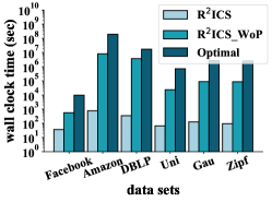
Figure 11. The R²ICS performance on real/synthetic graphs.

8.3. Ablation Study

To evaluate the effectiveness of our proposed pruning strategies, we conduct an ablation study over real/synthetic graphs, where all parameters are set to their default values. As shown in Figure LABEL:fig:ablation and LABEL:fig:ablation_time, we tested different combinations by adding one more pruning strategy each time: (1) keyword pruning only, (2) keyword + support pruning, and (3) keyword + support + influence score pruning. Figure LABEL:fig:ablation shows the number of pruned candidate communities for different pruning combinations, and Figure LABEL:fig:ablation_time shows the query time cost with different pruning combinations. From these figures, we can find that as more pruning strategies are used, the number of pruned communities increases by 1-3 orders of magnitude, and the wall clock time also decreases by 1 order of magnitude accordingly. Especially, the third influence score pruning strategy can significantly prune more candidate communities and reduce the query cost. On the other hand, due to the high density of the Facebook dataset, the number of pruned candidate communities for keyword and support pruning is zero. For Gaussian, since most of the vertices have the same keywords around the center vertex, the pruning power of the keyword pruning is zero.

8.4. Case Study

To evaluate the usefulness of our RICS results, we conduct a case study to compare the influences of the seed community obtained by our RICS approach with that by $k$-core (li2018persistent, ) over $DBLP$. Figure 13 shows the visualization of influence propagation between the seed community and the target community, where blue triangles are the vertices of the seed community, red stars are the vertices of the target community, and shades of edge color reflect influence scores. With the same target community, the left part of Figure 13 is the result of our RICS approach (4-truss), and the right part is the result of the $k$-core method (4-core). From this figure, we can find that although the 4-core community has more vertices, our RICS seed community has an influence score of 15.74, significantly greater than the 4.72 of the 4-core community. This confirms the usefulness of our RICS problem to obtain seed communities with high influences for real-world applications such as online advertising/marketing.

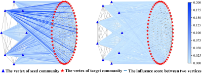
Figure 13. A case study of RICS with different community structures over DBLP dataset.

9. Related work

In this section, we briefly discuss research closely related to our work, specifically community search, community detection, and influence maximization.

Community Search (CS): The community search (CS) over social networks usually search for connected subgraphs containing a specific query vertex or a set of query vertices (fang2020survey, ; fang2020effective, ; sozio2010community, ). Some works (cui2014local, ; bonchi2019distance, ; batagelj2003m, ; zhang2019unboundedness, ; cui2013online, ) typically adopt cohesive subgraph models to measure the cohesiveness of subgraphs as a way to obtain a community from a query vertex $q$, such as $k$-core (bonchi2019distance, ; batagelj2003m, ), $k$-truss (zhang2019unboundedness, ; cohen2008trusses, ), $k$-clique (cui2013online, ; yuan2017index, ) and $k$-edge connectivity components (chang2015index, ; hu2017minimal, ). In (cui2014local, ; bonchi2019distance, ), the minimum degree was used to measure the cohesion of the $k$-core communities. In contrast, our RICS problem is more challenging in searching for densely structured communities and ensuring the high influence of communities with the constraint of query keywords. On the other hand, most studies on community search are searching from a certain user (forward search (sozio2010community, )), while our work focuses on reverse search starting from a certain community, which is more broadly considered and closer to real life.

Community Detection (CD): The community detection (CD) aims to detect all communities in a given social network. The foundation of many detection algorithms lies in graph partitioning (kernighan1970efficient, ; newman2013community, ) and clustering (girvan2002community, ; clauset2004finding, ; blondel2008fast, ). The Kernighan-Lin algorithm (kernighan1970efficient, ) is one of the earliest techniques used for graph partitioning, which divides the nodes of the graph into smaller components with specific attributes while minimizing the number of cut edges. Newman’s maximum likelihood algorithm (newman2013community, ), on the other hand, reduces the community detection problem to searching among a set of candidate solutions, each of which is a solution to the minimum cut graph partitioning. For the clustering method, Blondel et al. (blondel2008fast, ) presents a hierarchical clustering approach to address the CD problem, while Clauset et al. (clauset2004finding, ) notice modularity optimization and propose a greedy modularity optimization strategy to solve the CD problem. Different from CD, our RICS problem requires not just detecting communities but also finding the seed community that has the most influence on the target community.

Influence Maximization (IM): The influence maximization (IM) problem has been studied for a long time, which identifies a set of users as seed vertices with the maximum impact on other users within a given social network. Two influence propagation models proposed by Kempe et al. (kempe2003maximizing, ), the Independent Cascade (IC) model and the Linear Threshold (LT) model, have been widely used as influence propagation models for addressing influence maximization problems (chen2010scalable, ; wang2012scalable, ; chen2015online, ; li2015real, ). Chen et al. (chen2010scalable, ) introduces the DegreeDiscount heuristic algorithm for LT, presenting a scalable influence maximization algorithm. (wang2012scalable, ) proposed the PMIA heuristic algorithm for the IC model. However, such IM problems typically ignore the constraints among seed vertices, whereas our RICS problem pays attention to identifying seed communities that can influence the given target user group.

10. Conclusion

This paper proposed a novel RICS problem, which returns a seed community with the maximum influence on a user-specified target community. Unlike existing works, the RICS problem considers the influence of seed community on a specific user group/community rather than arbitrary users in social networks. To solve the RICS problem, we designed effective pruning strategies to filter out false alarms of candidate seed communities, and constructed an index to facilitate our proposed efficient RICS query processing algorithm. We also formulated and tackled a variant of RICS (i.e., R²ICS) by proposing an online query algorithm with effective vertex-to-community influence score pruning. Extensive experiments on real/synthetic social networks validated the efficiency and effectiveness of our RICS and R²ICS approaches.

References

- (1) Sijing Tu and Stefan Neumann. A viral marketing-based model for opinion dynamics in online social networks. In Proceedings of the Web Conference, pages 1570–1578, 2022.
- (2) Pejman Ebrahimi, Marjan Basirat, Ali Yousefi, Md Nekmahmud, Abbas Gholampour, and Maria Fekete-Farkas. Social networks marketing and consumer purchase behavior: the combination of sem and unsupervised machine learning approaches. Big Data and Cognitive Computing, 6(2):35, 2022.
- (3) Niranjan Rai and Xiang Lian. Top- community similarity search over large-scale road networks. IEEE Transactions on Knowledge and Data Engineering (TKDE), 35(10):10710–10721, 2023.
- (4) Reza Molaei, Kheirollah Rahsepar Fard, and Asgarali Bouyer. Time and cost-effective online advertising in social internet of things using influence maximization problem. Wirel. Networks, 30(2):695–710, 2024.
- (5) Sanjay Kumar, Abhishek Mallik, Anavi Khetarpal, and BS Panda. Influence maximization in social networks using graph embedding and graph neural network. Information Sciences, 607:1617–1636, 2022.
- (6) Neelakandan Subramani, Sathishkumar Veerappampalayam Easwaramoorthy, Prakash Mohan, Malliga Subramanian, and Velmurugan Sambath. A gradient boosted decision tree-based influencer prediction in social network analysis. Big Data and Cognitive Computing, 7(1):6, 2023.
- (7) Rong-Hua Li, Lu Qin, Jeffrey Xu Yu, and Rui Mao. Influential community search in large networks. Proceedings of the VLDB Endowment, 8(5):509–520, 2015.
- (8) Ruidong Yan, Deying Li, Weili Wu, Ding-Zhu Du, and Yongcai Wang. Minimizing influence of rumors by blockers on social networks: Algorithms and analysis. IEEE Trans. Netw. Sci. Eng., 7(3):1067–1078, 2020.
- (9) Yingli Zhou, Yixiang Fang, Wensheng Luo, and Yunming Ye. Influential community search over large heterogeneous information networks. Proceedings of the VLDB Endowment, 16(8):2047–2060, 2023.
- (10) Md Saiful Islam, Mohammed Eunus Ali, Yong-Bin Kang, Timos Sellis, Farhana M Choudhury, and Shamik Roy. Keyword aware influential community search in large attributed graphs. Information Systems, 104:101914, 2022.
- (11) Yanping Wu, Jun Zhao, Renjie Sun, Chen Chen, and Xiaoyang Wang. Efficient personalized influential community search in large networks. Data Science and Engineering, 6(3):310–322, 2021.
- (12) Ahmed Al-Baghdadi and Xiang Lian. Topic-based community search over spatial-social networks. Proceedings of the VLDB Endowment, 13(12):2104–2117, 2020.
- (13) Dengshi Li, Lu Zeng, Ruimin Hu, Xiaocong Liang, and Yilong Zang. Itc: Influential-truss community search. In 2022 International Joint Conference on Neural Networks (IJCNN), pages 01–08, 2022.
- (14) Jian Xu, Xiaoyi Fu, Yiming Wu, Ming Luo, Ming Xu, and Ning Zheng. Personalized top-n influential community search over large social networks. World Wide Web (WWW), 23:2153–2184, 2020.
- (15) Quan Fang, Jitao Sang, Changsheng Xu, and Yong Rui. Topic-sensitive influencer mining in interest-based social media networks via hypergraph learning. IEEE Transactions on Multimedia, 16(3):796–812, 2014.
- (16) Simon M Firestone, Michael P Ward, Robert M Christley, and Navneet K Dhand. The importance of location in contact networks: Describing early epidemic spread using spatial social network analysis. Preventive Veterinary Medicine, 102(3):185–195, 2011.
- (17) Huiyu Min, Jiuxin Cao, Tangfei Yuan, and Bo Liu. Topic based time-sensitive influence maximization in online social networks. World Wide Web (WWW), 23:1831–1859, 2020.
- (18) Khurshed Ali, Chih-Yu Wang, and Yi-Shin Chen. Leveraging transfer learning in reinforcement learning to tackle competitive influence maximization. Knowledge and Information Systems, 64(8):2059–2090, 2022.
- (19) Wei Chen, Yajun Wang, and Siyu Yang. Efficient influence maximization in social networks. In Proceedings of the International Conference on Knowledge Discovery and Data Mining, pages 199–208, 2009.
- (20) Wei Chen, Chi Wang, and Yajun Wang. Scalable influence maximization for prevalent viral marketing in large-scale social networks. In Proceedings of the International Conference on Knowledge Discovery and Data Mining (SIGKDD), pages 1029–1038, 2010.
- (21) Jonathan Cohen. Trusses: Cohesive subgraphs for social network analysis. National Security Agency Technical Report, 16(3.1), 2008.
- (22) Xin Huang and Laks VS Lakshmanan. Attribute-driven community search. Proceedings of the VLDB Endowment, 10(9):949–960, 2017.
- (23) George Karypis and Vipin Kumar. A fast and high quality multilevel scheme for partitioning irregular graphs. SIAM Journal on Scientific Computing, 20(1):359–392, 1998.
- (24) David A. Plaisted. Heuristic matching for graphs satisfying the triangle inequality. J. Algorithms, 5(2):163–179, 1984.
- (25) Jure Leskovec and Julian Mcauley. In Learning to discover social circles in ego networks, pages 548–556, 2012.
- (26) Jaewon Yang and Jure Leskovec. Defining and evaluating network communities based on ground-truth. In Proceedings of the ACM SIGKDD Workshop on Mining Data Semantics, pages 1–8, 2012.
- (27) Yang Zhou, Hong Cheng, and Jeffrey Xu Yu. Graph clustering based on structural/attribute similarities. Proceedings of the VLDB Endowment, 2(1):718–729, 2009.
- (28) Mark EJ Newman and Duncan J Watts. Renormalization group analysis of the small-world network model. Physics Letters A, 263(4-6):341–346, 1999.
- (29) Rong-Hua Li, Jiao Su, Lu Qin, Jeffrey Xu Yu, and Qiangqiang Dai. Persistent community search in temporal networks. In Proceedings of the International Conference on Data Engineering (ICDE), pages 797–808, 2018.
- (30) Yixiang Fang, Xin Huang, Lu Qin, Ying Zhang, Wenjie Zhang, Reynold Cheng, and Xuemin Lin. A survey of community search over big graphs. The VLDB Journal, 29:353–392, 2020.
- (31) Yixiang Fang, Yixing Yang, Wenjie Zhang, Xuemin Lin, and Xin Cao. Effective and efficient community search over large heterogeneous information networks. Proceedings of the VLDB Endowment, 13(6):854–867, 2020.
- (32) Mauro Sozio and Aristides Gionis. The community-search problem and how to plan a successful cocktail party. In Proceedings of the International Conference on Knowledge Discovery and Data Mining, pages 939–948, 2010.
- (33) Wanyun Cui, Yanghua Xiao, Haixun Wang, and Wei Wang. Local search of communities in large graphs. In Proceedings of the International Conference on Management of Data (SIGMOD), pages 991–1002, 2014.
- (34) Francesco Bonchi, Arijit Khan, and Lorenzo Severini. Distance-generalized core decomposition. In proceedings of the International Conference on Management of Data (SIGMOD), pages 1006–1023, 2019.
- (35) Vladimir Batagelj and Matjaz Zaversnik. An o (m) algorithm for cores decomposition of networks. arXiv preprint cs/0310049, 2003.
- (36) Yikai Zhang and Jeffrey Xu Yu. Unboundedness and efficiency of truss maintenance in evolving graphs. In Proceedings of the International Conference on Management of Data (SIGMOD), pages 1024–1041, 2019.
- (37) Wanyun Cui, Yanghua Xiao, Haixun Wang, Yiqi Lu, and Wei Wang. Online search of overlapping communities. In Proceedings of the International Conference on Management of Data (SIGMOD), pages 277–288, 2013.
- (38) Long Yuan, Lu Qin, Wenjie Zhang, Lijun Chang, and Jianye Yang. Index-based densest clique percolation community search in networks. IEEE Transactions on Knowledge and Data Engineering (TKDE), 30(5):922–935, 2017.
- (39) Lijun Chang, Xuemin Lin, Lu Qin, Jeffrey Xu Yu, and Wenjie Zhang. Index-based optimal algorithms for computing steiner components with maximum connectivity. In Proceedings of the International Conference on Management of Data (SIGMOD), pages 459–474, 2015.
- (40) Jiafeng Hu, Xiaowei Wu, Reynold Cheng, Siqiang Luo, and Yixiang Fang. On minimal steiner maximum-connected subgraph queries. IEEE Transactions on Knowledge and Data Engineering (TKDE), 29(11):2455–2469, 2017.
- (41) Brian W Kernighan and Shen Lin. An efficient heuristic procedure for partitioning graphs. The Bell system technical journal, 49(2):291–307, 1970.
- (42) Mark EJ Newman. Community detection and graph partitioning. Europhysics Letters, 103(2):28003, 2013.
- (43) Michelle Girvan and Mark EJ Newman. Community structure in social and biological networks. Proceedings of the National Academy of Sciences (PNAS), 99(12):7821–7826, 2002.
- (44) Aaron Clauset, Mark EJ Newman, and Cristopher Moore. Finding community structure in very large networks. Physical Review E, 70(6):066111, 2004.
- (45) Vincent D Blondel, Jean-Loup Guillaume, Renaud Lambiotte, and Etienne Lefebvre. Fast unfolding of communities in large networks. Journal of Statistical Mechanics: Theory and Experiment, 2008(10):P10008, 2008.
- (46) David Kempe, Jon Kleinberg, and Éva Tardos. Maximizing the spread of influence through a social network. In Proceedings of the International Conference on Knowledge Discovery and Data Mining (SIGKDD), pages 137–146, 2003.
- (47) Chi Wang, Wei Chen, and Yajun Wang. Scalable influence maximization for independent cascade model in large-scale social networks. Data Mining and Knowledge Discovery, 25:545–576, 2012.
- (48) Shuo Chen, Ju Fan, Guoliang Li, Jianhua Feng, Kian-lee Tan, and Jinhui Tang. Online topic-aware influence maximization. Proceedings of the VLDB Endowment, 8(6):666–677, 2015.
- (49) Yuchen Li, Dongxiang Zhang, and Kian-Lee Tan. Real-time targeted influence maximization for online advertisements. Proc. VLDB Endow., 8(10):1070–1081, 2015.