A STATISTICAL METHOD FOR IMPROVING MOMENTUM MEASUREMENT OF PHOTON CONVERSIONS RECONSTRUCTED FROM SINGLE ELECTRONS

Abstract

The reconstruction of photon conversions is importantin order to improve the reconstruction efficiency of the physics measurements involving photons. However, there are significant number of conversions in which only one of the two tracks emitted electrons is reconstructed in the detector due to very asymmetric energy sharing between the electron-positron pair. The momentum determination of the parent photon can be improved by estimating the missing energy in such conversions. In this study, we propose a simple statistical method that can be used to determine the mean value of the missing energy. By using simulated minimum bias events at LHC conditions and a toy detector simulation, the performance of the method is tested for several decay channels commonly used in particle physics analyses. A considerable improvement in the mass reconstruction precision is obtained when reconstructing particles decaying to photons whose energies are less than 20 GeV.

1 Introduction

In a photon conversion, usually an electron-positron pair is produced when a photon of enough energy interacts with a nucleus. In high-energy collision experiments, one has high photon multiplicity in an event leading to production of many photon conversion candidates within the detector material. Therefore, the reconstruction of photon conversions in particle detectors becomes important for a variety of physics analysis involving electromagnetic decay products such as $\pi^{0}\rightarrow\gamma\gamma$. The conversion reconstruction may also be used for detector-related studies. For example, mapping the distribution of the conversion vertices allows one to produce a precise localization of the material in the tracker detectors [1, 2].

Some fraction of the photon conversions will be highly asymmetric due to the energy sharing mechanism between the products. Either the electron ($e^{-}$) or the positron ($e^{+}$) can be produced with a very low energy. If this energy falls below a threshold required to produce a reconstructible track in the detector then the converted photon will be seen to have only one track and this type of conversion can be called a single electron conversion or a single track conversion. Even though there is a missing energy in such conversions, one can still use them to increase the efficiency of the reconstructed photons.

The missing energy of the unreconstructed track cannot be predicted kinematically since the parent photon energy is also unknown. However, for a large collection of the reconstructed tracks, the mean value of the missing energy can be evaluated as a function of the reconstructed energy and pseudo-rapidity. This paper describes a statistical procedure to estimate the missing energy in a single track photon conversion. By using the simulated minimum bias events at LHC conditions and a suitable toy detector simulation, the performance of the method is examined for the decay channels $\pi^{0}\rightarrow\gamma\gamma$, $\eta^{0}\rightarrow\gamma\gamma$ and $D^{*0}\rightarrow D^{0}\gamma$ and remarkable improvements in the mass reconstruction accuracies are observed.

The physics and reconstruction of photon conversion are given in Section 2 and 3 respectively. Section 4 describes the event and detector simulation selected for the study. The statistical method is introduced in Section 5. The performance of the method is presented in Section 6. Finally, a conclusion is given in Section 7.

2 Physics of photon conversion

At photon energies above 1 GeV, the interaction of the photons with a material will be dominated by $e^{-}e^{+}$ pair production. The photo-electric effect as well as the Rayleigh and Compton scattering cross sections are orders of magnitude below that of the photon conversion.

A detailed description for the cross section of the photon conversion process can be found in [3] and in the GEANT4 Physics Reference Manual [4]. Here, a relatively simplified model is used as described in [5]. Accordingly, for the photon energies used in this study ($E_{\gamma}>1$ GeV), the differential cross section can be approximated by:

$$\frac{d\sigma}{dx}=\frac{A}{X_{0}N_{A}}(1-\frac{4}{3}x(1-x))$$ (1)

where $x=E_{e}/E_{\gamma}$ is known as the fractional electron energy or the energy sharing, $A$ is the atomic mass in g/mol and $N_{A}$ is the Avogadro’s number. $X_{0}$ is the radiation length in g/cm² along the path of the photon. For a material whose atomic number is $Z$, $X_{0}$ can be evaluated from:

$$X_{0}=\frac{716.4~{}A}{Z(Z+1)\ln(287/\sqrt{Z})}$$ (2)

One can show that the total cross section is independent of the incident photon energy and given by:

$$\sigma_{\text{tot}}=\int_{0}^{1}{\frac{d\sigma}{dx}dx}=\frac{7A}{9X_{0}N_{A}}$$ (3)

Also, a normalized distribution of $x$ can be obtained from:

$$\rho(x)=\frac{1}{\sigma_{tot}}\frac{d\sigma}{dx}=\frac{9}{7}(1-\frac{4}{3}x(1-x))$$ (4)

Here $\rho(x)$ is symmetric function in $x$ and $1-x$, the electron and positron energies respectively. Since $x$ can have any random real value in the range $(0,1)$, the incident photon energy is not normally shared equally between the electron and positron. Hence, the single track photon conversion may turn out as a result of photons with a very asymmetric energy sharing between the electron and the positron.

At the reconstruction level, a transverse momentum cut, $p_{T,\text{cut}}$, is applied to form a list of good charged track candidates in an event. For example, $p_{T}>0.5$ GeV/c is required in many analyses at LHC conditions. However, the use of $p_{T,\text{cut}}$ results in an angular dependence in the reconstruction of the photon conversion process as follows. The probability of observing a single track photon conversion can be defined as:

$$P(x<x_{t})=\int_{0}^{x_{t}}\rho(x)dx$$ (5)

where $x_{t}=p_{T,\text{cut}}\cosh\eta/E_{\gamma}$ is the threshold value of the energy sharing and $\eta$ is the pseudo-rapidity of the parent photon. It can be shown that the single track conversion occurs more likely at lower photon energies and/or at higher $\eta$ values.

3 Reconstruction of photon conversion

The signatures of charged particles are usually obtained from the layered hit information in tracking detectors. As an example, the ATLAS Inner Detector is a composite tracking system consisting of pixels, silicon strips and straw tubes in a 2 T magnetic field. The tracking procedure selects track candidates with transverse momenta above 0.5 GeV/c. As for electrons, their energies can be determined from the energy deposition in the electromagnetic calorimeter. This measurement is combined with the measurement of the electron momentum in the inner detector to improve the energy resolution [6, 7].

In order to reconstruct the photon conversions a special vertex finding and fitting algorithm is used. This algorithm combines oppositely charged tracks in the event to evaluate the momenta of the conversion products at a vertex point in the detector. Since the converted photon is a massless particle, it also applies an additional angular constraint such that the two tracks produced at the vertex should have an initial difference of zero in their azimuthal and polar angles [8]. At the end of this procedure, one has a list of double track photon conversion candidates in the event.

The remaining tracks can be re-examined to collect possible single track conversions. In ATLAS, an electron-like track having its first hit beyond the pixel vertexing layer is a well known signature of the surviving leg of the single track conversion. Also, in rare cases, the conversion may happen so far from the beam axis that the conversion pair can merge. If they do not traverse a long enough distance inside the tracker, they cannot be resolved and as a result a single track is reconstructed [1, 8]. The other issue is to determine the production point of the single track conversion. Actually, there is no way to know the precise position because it may occur somewhere between detector layers (on the cables, on the cooling pipes etc). By definition, one can set the position of the single conversion to the first hit on the track.

4 Event and detector simulation

For the aim of the study the Pythia 8.1 tune 4cx event generator [9, 10] under LHC conditions (p-p collisions at the center of mass energy of 14 TeV) is used to generate about 200,000 events with the minimum bias processes. The simulated samples have additional collision events, pile-up, added such that the average number of interactions per event is 22. Also, the position of the interaction point is smeared around the origin by Gaussian distributions in $x$, $y$ and $z$, such that the widths are selected as $\sigma_{x}=\sigma_{y}=0.05$ mm and $\sigma_{z}=60$ mm.

The selected events are passed through a toy detector simulation. The momentum resolution is simulated by a single Gaussian smearing the momentum of the charged tracks as follows:

$$\sigma_{p_{T}}/p_{T}=Ap_{T}\oplus B$$ (6)

where the transverse momentum, $p_{T}$, is in GeV/c and $A$ and $B$ are numerical constants. In this study, ATLAS detector parameterization where $A=0.05\%$ and B = 1% is used [1]. The reconstructed charged particles are required to have the pseudo-rapidity $|\eta|<2.5$ and transverse momentum $p_{T}>0.5$ GeV/c.

The behavior of electrons in the detector is dominated by the radiative energy losses (bremsstrahlung) as they traverse the matter. Bremsstrahlung is a highly non-Gaussian process and cannot be adequately represented by a single Gaussian function as in Equation 6. In this study, the bremsstrahlung losses are modeled by a sum of three Gaussians to smear the electrons’ momenta in an event. This idea is extracted from the Gaussian Sum Filter approach [11] which is successfully applied to improve the track parameters of electrons both in ATLAS [12] and in CMS [13] experiments. Figure 1 shows an example of the relative residual distribution of the electrons where $p_{e}$ is the reconstructed momentum and $p_{true}$ is the true momentum at the generator level. The distribution has a Gaussian core and a large tail to negative values caused by radiative energy losses of the electrons. The mean values of the three Gaussian functions are required to be decreasing such that the first Gaussian function always describes the peak region of the distribution at around zero.

In the simulation, we have assumed that the tracking detector has 20 very long barrel layers which are regularly separated by 20 mm. All photons with $E_{\gamma}>1$ GeV in an event are converted at a random position between $r=[20~{}\text{mm},440~{}\text{mm}]$ where $r$ is the conversion radius measured from the beam axis. The cartesian coordinates of the conversion point can be found by extrapolating a line from the true photon production point to a cylindrical surface of radius $r^{\prime}$ which is the radius of the closest detector layer just after the conversion point along the path of the photon. Finally, the direction of the conversion products are assumed to be the same as the parent photon.

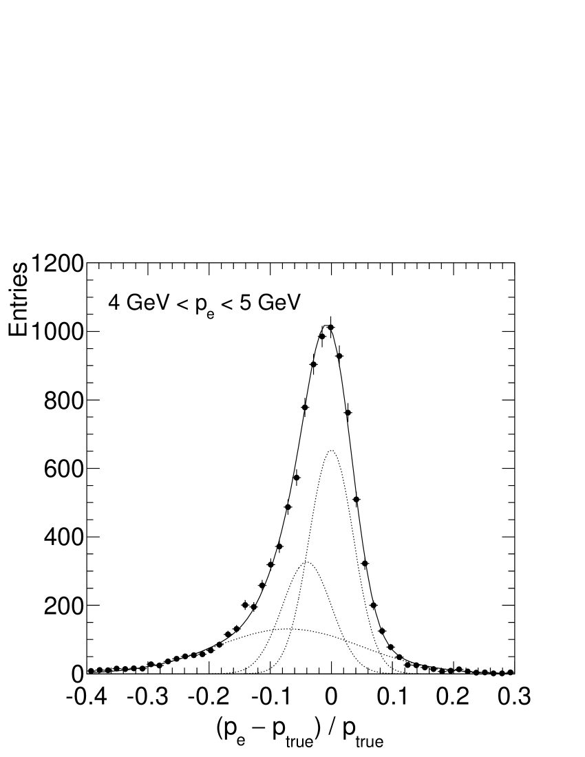
Figure 1: Example of the relative residual distribution of electrons for a given momentum range and for all eta bins. Data points are simulated with a sum of three normal distributions with the first Gaussian function forced to describe the peak region and the second and third Gaussian functions to model the tail to negative values.

5 The statistical correction method

In this section, the statistical method for compensating the missing energy in a single track conversion is discussed. The mass of the electron and the recoiling kinetic energy of the nucleus are neglected in the calculations.

In the single track conversion, the conservation of energy yields:

$$E_{\gamma}=E_{\text{reco}}+E_{\text{miss}}$$ (7)

where $E_{\text{reco}}$ is the reconstructed energy after applying the momentum smearing and transverse momentum cut and $E_{\text{miss}}$ is missing energy of the unreconstructed track at the truth level. In the most simple case one can assume that $E_{\text{miss}}=0$, i.e. the photon energy is carried only by the surviving track.

In fact, the missing energy can be estimated by a Monte Carlo study. For a given $p_{T\text{cut}}$, $E_{\text{miss}}$ will be distributed in the range $(0,~{}p_{T\text{cut}}\cosh\eta)$. Using a large enough number of minimum bias events, one can extract the mean value of the missing energy distribution, $\langle E_{\text{miss}}\rangle$, which is expected to be a function of the energy and pseudo-rapidity of the reconstructed track. Replacing $E_{\text{miss}}$ by $\langle E_{\text{miss}}\rangle$ in Equation 7 improves on average the value of $E_{\gamma}$.

Figure 2 shows an example missing energy distribution for $3.0~{}\text{GeV}<E_{\text{reco}}<4.0~{}\text{GeV}$, $2.0<|\eta|<2.2$ and $p_{T,\text{cut}}=0.5$ GeV/c². For these intervals, $\langle E_{\text{miss}}\rangle=0.665$ GeV and therefore the photon energy can be calculated simply from $E_{\gamma}=E_{\text{reco}}+0.665$ GeV.

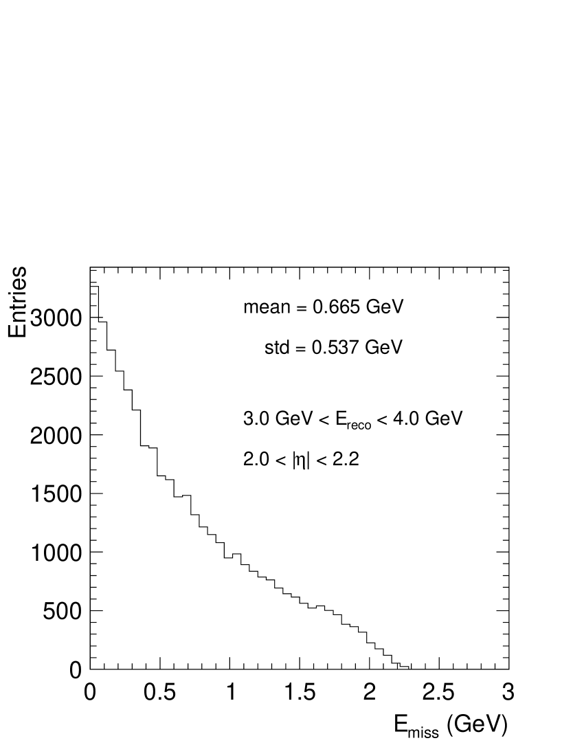
Figure 2: The missing energy distribution obtained from the Monte Carlo truth information for the specific reconstructed energy and pseudo-rapidity ranges.

In the study, 11 energy and 11 pseudo-rapidity intervals, given in Table 1, are defined for all single track conversions whose parent photons originate from any mother particle. A lego plot based on the $E_{\text{reco}}$ vs $\eta$ interval numbers, is shown in Figure 3 where the height of each bin stands for the mean value of the missing energy. These mean values are stored in a matrix for use in a physics analysis later. It is found that the values of the matrix elements depend on the detector resolutions and the kinematic cuts applied for selecting particles.

Table 1: The energy and pseudo-rapidity intervals defined for the reconstructed tracks in the conversions.

Interval	Energy (GeV)	Pseudo-rapidity
1	$0.50<E_{\text{reco}}<0.75$	$|\eta|<0.25$
2	$0.75<E_{\text{reco}}<1.00$	$0.25<|\eta|<0.50$
3	$1.00<E_{\text{reco}}<1.25$	$0.50<|\eta|<0.75$
4	$1.25<E_{\text{reco}}<1.50$	$0.75<|\eta|<1.00$
5	$1.50<E_{\text{reco}}<2.00$	$1.00<|\eta|<1.25$
6	$2.00<E_{\text{reco}}<3.00$	$1.25<|\eta|<1.50$
7	$3.00<E_{\text{reco}}<4.00$	$1.50<|\eta|<1.75$
8	$4.00<E_{\text{reco}}<5.00$	$1.75<|\eta|<2.00$
9	$5.00<E_{\text{reco}}<7.50$	$2.00<|\eta|<2.20$
10	$7.50<E_{\text{reco}}<10.0$	$2.20<|\eta|<2.40$
11	$10.0<E_{\text{reco}}<20.0$	$2.40<|\eta|<2.50$

Figure 3: The lego plot indicating the values of the missing energy matrix elements ($\langle E_{\text{miss}}\rangle$) obtained from the Monte Carlo truth study as a function of the reconstructed energy and pseudo-rapidity interval numbers given in Table 1. There are relatively larger fluctuations in lower energy and pseudo-rapidity intervals.

The final issue is to determine the direction of the parent photon which is defined in two ways. First, it can be considered as having the same direction of the reconstructed track. In this case, the four-vector of the photon can be defined as:

$$P_{\gamma}=(E_{\gamma}\frac{p_{x,\text{reco}}}{p_{\text{reco}}},~{}E_{\gamma}\frac{p_{y,\text{reco}}}{p_{\text{reco}}},~{}E_{\gamma}\frac{p_{z,\text{reco}}}{p_{\text{reco}}},~{}E_{\gamma})$$ (8)

where $p_{x,y,z,\text{reco}}$ are the xyz-components of the momentum at the production point and $p_{\text{reco}}\approx E_{\text{reco}}$ is the magnitude of the momentum of the reconstructed track. Second, one can assume that the photon is originating from the primary vertex in the event. Then, the photon will be in the direction of the line joining the primary vertex $A=(x_{0},~{}y_{0},~{}z_{0})$ to the pair production point $B=(x_{p},~{}y_{p},~{}z_{p})$. In our toy simulation, we set $A=(0,~{}0,~{}0)$. This approach yields a four-vector:

$$P_{\gamma}=(E_{\gamma}\frac{x_{p}}{R_{p}},~{}E_{\gamma}\frac{y_{p}}{R_{p}},~{}E_{\gamma}\frac{z_{p}}{R_{p}},~{}E_{\gamma})$$ (9)

where $R_{p}=|AB|=(x_{p}^{2}+y_{p}^{2}+z_{p}^{2})^{1/2}$. No significant difference is observed between the use of the equations  8 and 9 in the simulation.

To avoid biases in the training data (over-training), the missing energy matrix is produced by using a training data set which is the first half of the full data. The validation of the method is performed using an independent test data which is the rest of the full data. The use of single track photon conversions in our analysis is summarized in the following algorithm.

1. Generate an event.

2. Select a photon from any source in the event.

3. Convert the photon at a random point in the detector.

4. Obtain the energy of the electron and positron from the distribution given in Equation 4.

5. Smear the momentum of the electron and positron and determine their four-vectors whose space coordinates are in the direction of the photon.

6. If one of the energy of the conversion products falls below the threshold, evaluate the value of the reconstructed energy, $E_{\text{reco}}$, and the value of $\langle E_{\text{miss}}\rangle$ from the mean missing energy matrix depending on $E_{\text{reco}}$ and $\eta$.

7. Compute the energy of the reconstructed photon from $E_{\gamma}=E_{\text{reco}}+\langle E_{\text{miss}}\rangle$ and evaluate its four-vector from Equation 8.

8. Use the reconstructed photon in the analysis.

6 Performance

The performance of the statistical procedure given in the previous section is tested for three different decay channels. The nominal mass of each particle is taken from Ref [14] and, the transverse momentum cut is taken as $p_{T,\text{cut}}=0.5$ GeV/c unless otherwise stated.

6.1 Invariant mass distributions

Firstly, the common decays containing two photons, $\pi^{0}\rightarrow\gamma\gamma$ and $\eta^{0}\rightarrow\gamma\gamma$, are considered. For the reconstructed photon energies $E_{1}$ and $E_{2}$, the two-photon invariant mass is defined by:

$$M_{\gamma\gamma}=\sqrt{2E_{1}E_{2}(1-\cos\theta)}$$ (10)

where $\theta$ is the opening angle between photons. Figure 4a and 4b respectively show $M_{\gamma\gamma}$ distributions of $\pi^{0}$ and $\eta^{0}$ signals for $E_{\text{miss}}=0$ and $E_{\text{miss}}=\langle E_{\text{miss}}\rangle$ where both photons are built from the single track conversion. The photon energies, $E_{1}$ and $E_{2}$, tend to have lower values when $E_{\text{miss}}=0$. As a result, $\pi^{0}$ and $\eta^{0}$ signals are shifted to lower mass values according to Equation 10. However, by correcting the missing energy, the mean of the distributions are moved to their nominal positions as indicated by the dashed lines on the figures. The peak regions of both signals are fitted to Gaussian functions. The center positions and widths of the fits are shown as mean and std respectively on the figure.

The same procedure is repeated for the decay $D^{*0}\rightarrow D^{0}\gamma$ where $D^{0}$ candidates are selected from the channel $D^{0}\rightarrow K^{\pm}\pi^{\mp}$. The three-particle invariant mass, $M_{K,~{}\pi,~{}\gamma}$, distributions before and after correction are shown in Figure 5a and  5b respectively. It is clear that the mean correction method improves the accuracy of the $D^{*0}$ mass reconstruction.

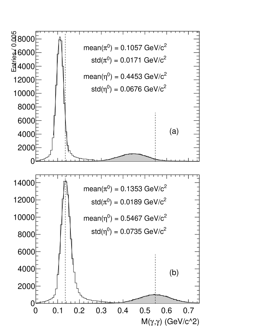
Figure 4: Two-photon invariant mass spectra for $\pi^{0}$ and $\eta^{0}$ signals, where both photons are reconstructed from the single track conversion, when (a) $E_{\text{miss}}=0$ and (b) $E_{\text{miss}}=\langle E_{\text{miss}}\rangle$. The nominal mass positions, $M_{\pi^{0}}=0.1349766$ GeV/c² and $M_{\eta^{0}}=0.547862$ GeV/c², are indicated by the dashed lines. mean and std represent respectively the center and the width of the Gaussian fits.

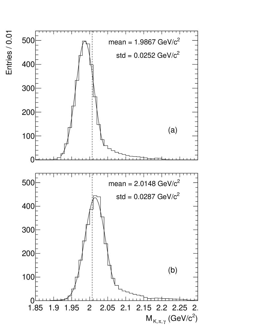
Figure 5: $M_{K~{}\pi,~{}\gamma}$ spectra for $D^{*0}$ signal where the photon is reconstructed from the single track conversion, when (a) $E_{\text{miss}}=0$ and (b) $E_{\text{miss}}=\langle E_{\text{miss}}\rangle$. The nominal mass position, $M_{D^{*0}}=2.00699$ GeV/c², is indicated by a dashed line. mean and std represent respectively the center and the width of the Gaussian fits.

6.2 Energy resolution

The energy resolution of the photons can be extracted from the standard deviation of the relative residual distribution defined by $(E_{\gamma}-E_{true})/E_{true}$ where $E_{true}$ is the true photon energy at the generator level. Figure 6 shows the relative residual distribution of photons reconstructed from single track conversions before and after missing energy correction. Clearly, the distribution is asymmetric with negative mean value when no correction is applied. However, the proposed method shifts the mean of the distribution to around zero while its width is slightly wider.

Similar relative residual distributions can be obtained for the momenta of parent particles decaying to photons built from single track conversions. However, further improvement in the parent’s momentum can be obtained by applying a mass constraint as described in [15] for example.

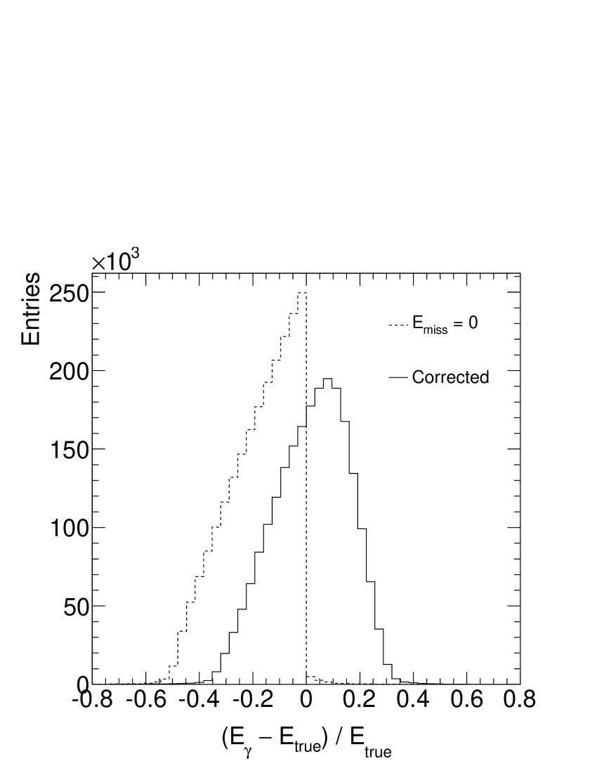
Figure 6: The relative residual distributions of photons built from single track conversions for all photon energy and pseudo-rapidity intervals.

6.3 Size of energy and $\eta$ bins

In order to investigate how much the results depend on the binning choice, coarser bins including only 6 energy and 6 pseudo-rapidity intervals are defined such that the range of each interval in Table 1 is doubled.

Figure 7 shows three $\pi^{0}\rightarrow\gamma\gamma$ invariant mass distributions where both photons are reconstructed from single track conversions. The solid and dashed histograms are respectively obtained for the case $E_{\text{miss}}=\langle E_{\text{miss}}\rangle$ where bin type 1 represents the binning in Table 1, while bin type 2 represents the new energy and pseudo-rapidity bins. The coarser bin selection result in a slightly wider mass distribution. Hence, depending on the size of data, the selection of finer bins turns out a better mass reconstruction precision.

In addition, to compare the results with the best reconstruction scenario, one can choose $E_{\text{miss}}=E_{\text{true}}$. This is also shown as a shaded histogram in the same figure. Note that, in the perfect case, the true $\pi^{0}$ signal has still a significant mass resolution —FWHM of the perfect distribution is about 4 times narrower than the bin type 1. This is because the mass resolution is also affected by the opening angle resolution between the photons arising from the four-vector definition of single track conversions.

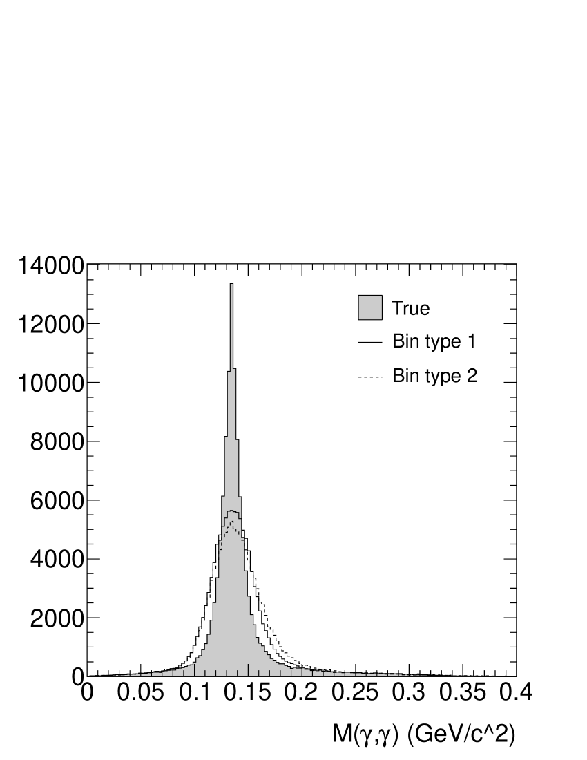
Figure 7: The effect of the selection of bin size on $\pi^{0}$ signal. bin 1 and bin 2 are respectively represent intervals defined in Table 1 and the other intervals defined in the text. The shaded histogram is obtained when $E_{\text{miss}}=E_{\text{true}}$.

6.4 Effect of $p_{T,\text{cut}}$

It is interesting to investigate the effect of $p_{T,\text{cut}}$ on the mean value and the energy resolution (width) of the residual distributions. As indicated in Figure 8a, the mean values obtained after the correction is slightly influenced by $p_{T,\text{cut}}$ and their values are close to zero. As we expect, the mean values are always negative and far from zero when no correction is applied.

Figure 8b shows the energy resolutions as a function of $p_{T,\text{cut}}$. Clearly, the resolutions are getting worse with increasing $p_{T,\text{cut}}$. A similar behaviour can be seen in Figure 8c which shows the evolution of $\langle E_{\text{miss}}\rangle$ for a specific $E_{\text{reco}}$ and $\eta$ bins. as a function of $p_{T,\text{cut}}$ up to 2 GeV/c. Therefore, in consideration of $p_{T,\text{cut}}$, the strong positive correlation between the energy resolution and $\langle E_{\text{miss}}\rangle$ points out that the overshooting in the energy correction of individual photons results in the loss in the energy resolution of single track conversions.

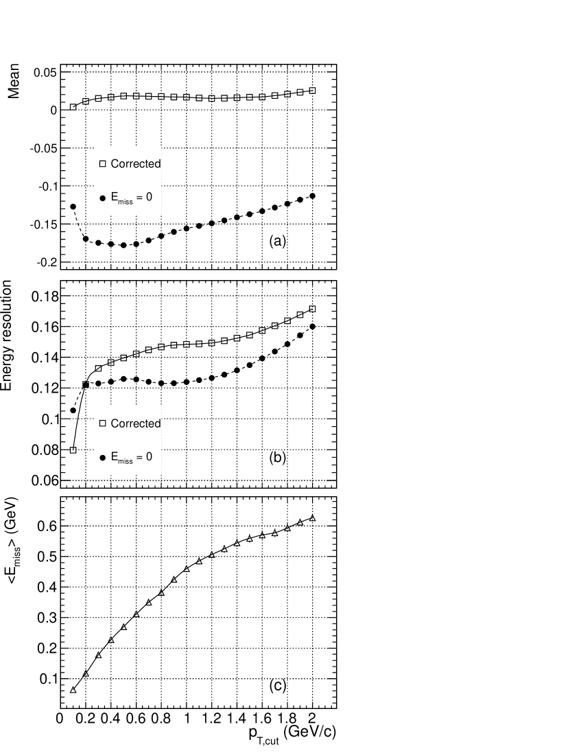
Figure 8: (a) The mean value and (b) the energy resolution extracted from the relative residual distributions as a function of $p_{T,\text{cut}}$. (c) The mean values of the missing energy for a specific energy and pseudo-rapidity intervals. for the same $p_{T,\text{cut}}$ values. Error bars are much less than the marker sizes.

7 Conclusion

In a photon conversion one of the electron track can be missed for various reasons. However, the reconstruction of such single-track photon conversions may be a major concern for a number of physics analyses involving photons especially at the LHC. In this study, a simple statistical method based on the average energy correction for determining the missing energy in single-track conversions has been introduced. By using the minimum bias events generated at LHC conditions and a toy detector simulation, the method is shown to perform well when it is applied to signal events like $\pi^{0}\rightarrow\gamma\gamma$ and $D^{*0}\rightarrow D^{0}\gamma$ where the resulting photons are built from single track conversions. It is found that the energy resolution of such photons are becoming worse with increasing the value of $p_{T,\text{cut}}$. However, the performance of the method may be improved by using finer energy and pseudo-rapidity bins.

The procedure described here can be implemented to improve the measurements and discovery potentials of rare decays such as $\Omega^{-}\rightarrow\Xi^{-}\gamma$ or $\Sigma^{0}\rightarrow\Lambda\gamma\gamma$. However, in a real analysis, the reader must also consider the background events acting as single track or double track photon conversions for instance $\pi^{0}\rightarrow e^{-}e^{+}\gamma$, $K^{0}_{S}\rightarrow\pi^{+}\pi^{-}$, $\Lambda\rightarrow p\pi$, $\Sigma^{+}\rightarrow p\gamma$ etc.

The statistical approach is clearly not useful for correcting individual photon momenta. However, the single-track photon conversions will still be highly desirable to improve the reconstruction efficiency of particles decaying to photons in an event. Therefore, a statistical approach similar to this study might be very useful for scientists working with photon data collected from experiments containing a high radiation length in the tracking detectors.

References

- [1] The ATLAS Collaboration, JINST 3 S08003 (2008)
- [2] The ATLAS Collaboration, JINST 6 P04001 (2011)
- [3] Y.S. Tsai, Rev. Mod. Phys. 46 (1974) 815-851
- [4] S. Agostinelli et al., Nucl. Instr. Meth. A 506 (2006) 250
- [5] S. R. Klein, Radiat. Phys. Chem. 75 (2006) 696
- [6] The ATLAS Collaboration, JHEP 1009:056, (2010)
- [7] The ATLAS Collaboration, JINST 5 P11006 (2010)
- [8] The ATLAS Collaboration, arXiv:0901.0512, CERN-OPEN-2008-020
- [9] T. Sjöstrand, S. Mrenna and T.Skands, Comput. Phys. Comm. 178 (2008) 852
- [10] R. Corke and T. Sjöstrand, JHEP 05 (2011) 009, arXiv:1101.5953 [hep-ph]
- [11] R. Frühwirth, Comp. Phys. Comm. 154 (2003) 131
- [12] The ATLAS Collaboration, Eur. Phys. J. C, 74, (2014) 3071.
- [13] W.Adam et al., J. Phys. G: Nucl. Part. Phys. 31 (2005) N9.N20
- [14] J. Beringer et al. (Particle Data Group), Phys. Rev. D86, 010001 (2012)
- [15] A. Bingül, Nucl. Instr. Meth. A 693 (2012) 11