Two competing populations with a common environmental resource

Abstract

Feedback-evolving games is a framework that models the co-evolution between payoff functions and an environmental state. It serves as a useful tool to analyze many social dilemmas such as natural resource consumption, behaviors in epidemics, and the evolution of biological populations. However, it has primarily focused on the dynamics of a single population of agents. In this paper, we consider the impact of two populations of agents that share a common environmental resource. We focus on a scenario where individuals in one population are governed by an environmentally “responsible” incentive policy, and individuals in the other population are environmentally “irresponsible”. An analysis on the asymptotic stability of the coupled system is provided, and conditions for which the resource collapses are identified. We then derive consumption rates for the irresponsible population that optimally exploit the environmental resource, and analyze how incentives should be allocated to the responsible population that most effectively promote the environment via a sensitivity analysis.

I Introduction

Classical game theory describes strategic interactions between individuals provided that the incentives for their choices are static, i.e. do not change over time. However, their choices often have an impact on a shared environment, which in turn may affect their incentives for future decisions. The utilization of common resources such as water, fishing grounds, or traffic networks best illustrates this – high individual utilization makes fewer resources available to others in the future [1]. Clearly, a dynamic interplay exists between users’ decisions and their impact on a shared environmental state.

The recent framework of feedback-evolving games addresses this interplay by incorporating a changing environmental state coupled with existing evolutionary game theoretic dynamics [2, 3, 4]. The core model considers payoff functions to individuals that depend on whether the environment is in an abundant or depleted state. It is primarily used to understand how the payoff functions should be structured in order to avoid a “tragedy of the commons”, an outcome in which the environment ultimately becomes depleted. In other words, these payoff functions reflect environmental incentive policies that can be designed to manage the common resource [5, 6, 7].

Much of the existing research focuses on a single population of agents whose decisions impact the environment in isolation [8, 9, 10, 7, 11, 12, 13]. These models are not sufficient to describe multi-population interactions. For example, individuals in neighboring countries follow different environmental policies, yet utilize resources from the same common source (e.g. fish in the ocean, water from rivers, clean air). Extensions of feedback-evolving games to multiple populations, and possibly multiple local environments, would enable a vastly richer set of scenarios for study. While some work has studied the dynamics of multi-population models in recent years [14, 15, 16], an interesting and understudied direction involves hierarchical decision-making, i.e. the strategic selection of local incentive policies, under the context that the activity from one population has externalities on resources utilized by other populations.

In this paper, we extend the framework in this direction by considering two populations that share the same local environmental resource. We focus on a particular setting where one population, labelled “responsible”, implements a pro-environmental incentive policy such that the common resource can be sustained in the absence of other populations. The other population, labelled “irresponsible”, does not restrain its consumption activity. Our study centers on the following question, stated informally as

To what extent can the irresponsible population exploit the environmental resource?

While too much consumption could cause the resource to collapse, too little consumption leaves missed opportunities. Our highlighted contributions are:

• A stability analysis for the dynamics of the two-population system.

• Identify conditions for which the environment collapses, and when it can be sustained.

• Derivation of the optimal consumption rates for the irresponsible population.

• A sensitivity analysis for the incentive policies chosen by the responsible population.

The last item above illustrates how incentives should be allocated in order to maximally promote the environmental resource. Interestingly, we find that incentivizing mutual cooperation (i.e. coordinated) is far more effective in promoting resource levels than incentivizing unilateral cooperation (anti-coordinated).

The paper is organized as follows. Section II provides relevant background on single population feedback-evolving games, before presenting the two-population model. Section III states our main result regarding the dynamics of the model. Section IV proposes and solves an optimization problem regarding the irresponsible population’s choice of consumption levels. Simulations and sensitivity analyses are given in Section V, followed by concluding remarks.

II Model

Before describing our two-population model, preliminary background on single-population feedback-evolving games is provided.

II-A Preliminary on Feedback-evolving games

A single-population feedback-evolving game describes a population of agents that have access to a degradable environmental resource. The relative abundance of the resource is denoted by $n\in[0,1]$. At any given time, each agent is choosing whether to use a low consumption action (strategy $\mathcal{L}$), or a high consumption action (strategy $\mathcal{H}$). High consumption degrades $n$, and low consumption improves $n$. The immediate payoff experienced by an agent is described by the environment-dependent $2\times 2$ payoff matrix,

$$A_{n}=n\begin{bmatrix}R_{1}&S_{1}\\ T_{1}&P_{1}\end{bmatrix}+(1-n)\begin{bmatrix}R_{0}&S_{0}\\ T_{0}&P_{0}\end{bmatrix}$$ (1)

Here, the first row and column corresponds to a low consumer, and the second row and column corresponds to a high consumer. Entry $ij$ ($i,j\in\{\mathcal{L},\mathcal{H}\}$) indicates the experienced payoff to an agent using strategy $i$ when encountering an agent using strategy $j$. We denote $x\in[0,1]$ as the fraction (or frequency) of agents in the population using strategy $\mathcal{L}$. The payoff experienced by each type of agent is then given by

$$\pi_{\mathcal{L}}(x,n)=[A_{n}[x,1-x]^{\top}]_{1},\quad\pi_{\mathcal{H}}(x,n)=[A_{n}[x,1-x]^{\top}]_{2}$$ (2)

The payoffs are determined by the parameters in the $A_{0}$ and $A_{1}$ matrices. The $A_{1}$ matrix is the payoff matrix when the environment is abundant. Following the literature on feedback-evolving games, we make the following assumption about the $A_{1}$ matrix.

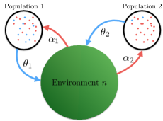
Figure 1: Diagram of our two-population model. Activities from both populations impact the shared environmental state, $n$. The rates $\theta_{i}$, $\alpha_{i}$ denote the restoration and degradation rates from the activities of population $i$, respectively.

Assumption 1.

High consumption is the dominant strategy in $A_{1}$, i.e. $\delta_{TR1}:=T_{1}-R_{1}>0$ and $\delta_{PS1}:=P_{1}-S_{1}>0$

On the other hand, the $A_{0}$ matrix describes payoffs when the environment is depleted. We interpret $A_{0}$ to be an “environmental policy” that the population has follows. For example, the low consumption strategy may be more incentivized when the environment is bad (e.g. subsidies for using electric vehicles). The payoff structure of the $A_{0}$ matrix is completely determined from the parameters $\delta_{SP0}:=S_{0}-P_{0}$ and $\delta_{RT0}:=R_{0}-T_{0}$.

We will use the replicator equation to describe how agents revise their decisions over time. Moreover, the environment $n$ evolves over time, as it is influenced by the decisions in the population. The overall system dynamics is given by two coupled ODEs:

$$\dot{x} =x(1-x)g(x,n)$$ (3)

$$\dot{n} =\epsilon n(1-n)(\theta x-\alpha(1-x))$$

where

$$g(x,n):=\pi_{\mathcal{L}}(x,n)-\pi_{\mathcal{H}}(x,n)$$ (4)

is the payoff difference between low and high consumers, $\theta>0$ is the restoration rate from low consumption activity, $\alpha>0$ is the degradation rate from high consumption activity, and $\epsilon>0$ is a time-scale separation constant. The form of the $\dot{n}$ equation is often referred to as the tipping point dynamics, since $n$ is increasing only if there are sufficiently high fraction of low consumers.

The state of the system $(x,n)$ evolves over the state space $[0,1]^{2}$. Indeed, the set $(0,1)^{2}$ is forward-invariant under the dynamics (3). The originating work [2] provided a full characterization of the asymptotic outcomes of system (3) for all possible environmental policy matrices $A_{0}$.

The result below summarizes the variety of behaviors that system (3) can exhibit.

Theorem 2.1 (adapted from [2]).

The environmental policy $(\delta_{SP0},\delta_{RT0})$ determines the asymptotic properties of (3) as follows.

1) Sustained resource: If $(\delta_{SP0},\delta_{RT0})\in\mathcal{V}$, where

$$\mathcal{V}:=\{(y_{1},y_{2})\in\mathbb{R}^{2}:y_{1}>0\text{ and }-\frac{\theta}{\alpha}y_{1}<y_{2}<\frac{\delta_{TR1}}{\delta_{PS1}}y_{1}\},$$ (5)

then the fixed point $(x^{*},n^{*})=(\frac{\alpha}{\alpha+\theta},\frac{g(x^{*},0)}{-\partial g/\partial n(x^{*})})\in(0,1)^{2}$ is the only asymptotically stable fixed point in the system.

2) Oscillating Tragedy of the commons: If $\delta_{SP0}>0$ and $\frac{\delta_{TR1}}{\delta_{PS1}}\delta_{SP0}<\delta_{RT0}$, then system (3) exhibits a stable heteroclinic cycle between the four corner fixed points, $(0,0)$, $(1,0)$, $(1,1)$, $(0,1)$.

3) Tragedy of the commons: If $\delta_{SP0}\leq 0$, or $\delta_{SP0}>0$ and $\delta_{RT0}<-\frac{\theta}{\alpha}\delta_{SP0}$, then the only asymptotically stable fixed point has $n=0$.

The environmental policies belonging to $\mathcal{V}$ are ones that can sustain a stable and non-zero resource level. In other words, they avert a tragedy of the commons [17], which refers to a fixed point where the resource level is zero. The policies in $\mathcal{V}$ can be considered as more desirable operating conditions than the policies described in items 2 and 3 above. The oscillating tragedy of the commons is considered an undesirable outcome, in which the system cycles between states of nearly zero resource levels, and states of fully abundant resource levels. Visually, the state trajectory “spirals outward” from the interior, and its $\omega$-limit set is the boundary of the state space.

II-B Model: Two-population feedback-evolving games

Now, we consider two populations that share the environmental resource. Figure 1 illustrates this scenario. Specifically, the consumption decisions of the members of both populations have effects on the environmental resource. Now, $x_{i}\in[0,1]$ denotes the fraction of low consumers in population $i\in\{1,2\}$. The behavior of population $i$ is governed by the payoff matrices $A_{0}^{(i)}$ (parameters $\delta_{SP0}^{i}$, $\delta_{RT0}^{i}$) and $A_{1}^{(i)}$ (parameters $\delta_{TR1}^{i}$, $\delta_{PS1}^{i}$), restoration rate $\theta_{i}>0$, degradation rate $\alpha_{i}>0$. In line with Assumption 1, we maintain the parameters in the abundant state satisfy $\delta_{TR1}^{i},\delta_{PS1}^{i}>0$. The payoff differences for each population are given by

$$g_{i}(x_{i},n):=\pi_{\mathcal{L}}^{(i)}(x_{i},n)-\pi_{\mathcal{H}}^{(i)}(x_{i},n)$$ (6)

where $\pi_{j}^{(i)}$ is the experienced payoff to a $j$-strategist in population $i$. The system dynamics are now given by the set of three ODEs with state variable $\boldsymbol{z}=(x_{1},x_{2},n)$:

$$\dot{x}_{1} =x_{1}(1-x_{1})g_{1}(x_{1},n)$$ (7)

$$\dot{x}_{2} =x_{2}(1-x_{2})g_{2}(x_{2},n)$$

$$\dot{n} =\epsilon n(1-n)h(x_{1},x_{2})$$

where $h(x_{1},x_{2}):=\sum_{i=1}^{2}(\theta_{i}x_{i}-\alpha_{i}(1-x_{i}))$, and with initial condition $(x_{1}(0),x_{2}(0),n(0))\in(0,1)^{3}$. By construction, $(0,1)^{3}$ is a forward-invariant set. We are interested in studying how the dynamics of the two-population environmental coupled system (7) behaves with respect to the population’s defining parameters – especially how the environmental policies $A_{0}^{(1)}$, $A_{0}^{(2)}$ adopted by each population affects environmental resources. We will make the following assumptions on these environmental policies.

Assumption 2.

We assume that $\frac{\partial g_{i}}{\partial n}(x_{i})<0$ for all $x_{i}\in[0,1]$, $i=1,2$. This is equivalent to $\delta_{SP0}^{i}>-\delta_{PS1}^{i}$ and $\delta_{RT0}^{i}>-\delta_{TR1}^{i}$.

Assumption 2 asserts that the relative payoff to low consumers in both populations monotonically decreases as the environmental state improves. The next and final assumption focuses our study on a scenario where one population is “environmentally responsible”, and the other population is “irresponsible”.

Assumption 3.

For population 1, we assume that $(\delta_{SP0}^{1},\delta_{RT0}^{1})\in\mathcal{V}$ (with $\theta=\theta_{1}$ and $\alpha=\alpha_{1}$). For population 2, we assume that $\delta_{SP0}^{2},\delta_{RT0}^{2}<0$.

The first part of Assumption 3 asserts that agents in population 1 are cooperative enough to sustain the resource (Theorem 2.1, item 1) in the absence of population 2. The second part asserts that agents in population 2 make no effort to conserve resources, always preferring the high consumption strategy. We will refer to population 1 as responsible, and population 2 as irresponsible. The set of all feasible policies specified by Assumptions 2 and 3 is visually depicted in Figure 2.

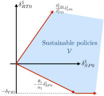
Figure 2: The set of all sustainable policies for population 1 is shown as the blue region. A sustainable policy maintains a stable, nonzero resource in the absence of other populations (Theorem 2.1). This region is the focus of Assumptions 2 and 3.

III Stability analysis of two-population game

In this section, we characterize the dynamical behavior of the two-population coupled system by analyzing the local stability properties of all of its fixed points.

Theorem 3.1.

The asymptotic dynamics of the two-population system (7) are summarized below.

1) Suppose $\alpha_{2}>\theta_{1}$. Then a tragedy of the commons is globally asymptotically stable, i.e. $\lim_{t\rightarrow\infty}n(t)=0$.

2) Suppose $\alpha_{2}\leq\theta_{1}$.

1. If $\frac{\alpha_{2}-\theta_{1}}{\alpha_{1}+\alpha_{2}}\delta_{SP0}^{1}\leq\delta_{RT0}^{1}\leq\frac{\delta_{TR1}}{\delta_{PS1}}\delta_{SP0}^{1}$, then the only asymptotically stable fixed point is of the form $(x_{1},0,n)$, where

   $$x_{1}^{*}:=\frac{\alpha_{1}+\alpha_{2}}{\alpha_{1}+\theta_{1}},\quad n^{*}:=-\frac{g_{1}(x_{1}^{*},0)}{\frac{\partial g_{1}}{\partial n}(x_{1}^{*})}.$$ (8)

2. If $\delta_{RT0}^{1}<\frac{\alpha_{2}-\theta_{1}}{\alpha_{1}+\alpha_{2}}\delta_{SP0}^{1}$, then the only asymptotically stable fixed point constitutes a tragedy of the commons.

Several remarks are in order. In item 1 above, the irresponsible population induces a tragedy of the commons if its consumption rate is higher than the responsible population’s restoration rate. Item 2a provides a region of sustainable policies for population 1. We note that this region gets smaller as $\alpha_{2}$ increases while remaining less than $\theta_{1}$.

Moreover, we observe the sustained resource level $n^{*}$ in item 2a is a decreasing function in $\alpha_{2}$. Taking the derivative with respect to $\alpha_{2}$, we obtain

$$\frac{\partial n^{*}}{\partial\alpha_{2}}=\frac{g_{1}(x_{1}^{*},0)\frac{\partial^{2}g_{1}}{\partial n\partial x}-\frac{\partial g_{1}}{\partial x}(x_{1}^{*},0)\frac{\partial g_{1}}{\partial n}(x_{1}^{*})}{(\alpha_{1}+\theta_{1})(\frac{\partial g_{1}}{\partial n}(x_{1}^{*}))^{2}}$$

It is negative since the numerator being negative is equivalent to the condition $\delta_{RT0}^{1}\leq\frac{\delta_{TR1}}{\delta_{PS1}}\delta_{SP0}^{1}$.

Item 2b provides a region where the population 1 policy fails to sustain the resource even though $\alpha_{2}<\theta_{1}$.

The proofs for each part of Theorem 3.1 are presented in Appendix -A.

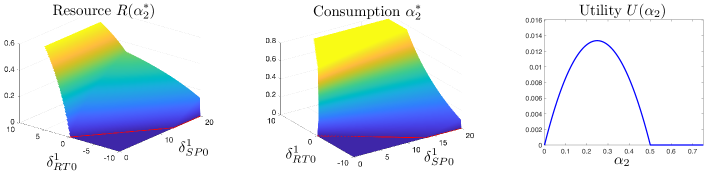
Figure 3: (Left) This surface plot shows the resource level that results from the optimal consumption rate $\alpha_{2}^{*}$ detailed in Theorem 4.1. The red line indicates the bottom border of the set of feasible policies for population 1. We observe that $R(\alpha_{2}^{*})$ is increasing in both $\delta_{RT0}^{1}$ and $\delta_{SP0}^{1}$. (Center) The optimal consumption rate detailed in Theorem 4.1. (Right) An example of the utility function $U_{2}(\alpha_{2})$ under policy $(\delta_{SP0}^{1},\delta_{RT0}^{1})=(3,-0.5)$. For all simulations, the parameter values are: $\delta_{TR1}=10$, $\delta_{PS1}=6$, $\theta_{1}=0.75$, $\alpha_{1}=1$, $\epsilon=0.1$.

IV Results: exploitation of resources

In this section, we study the following hierarchical decision problem posed informally as: how much consumption can the irresponsible population get away with? To approach this question, we consider a local authority for population 2 that may set the consumption rate $\alpha_{2}\geq 0$. This decision is representative of, for example, water usage or fishing regulations.

From Theorem 3.1, we succinctly summarize the resource level that results in the asymptotically stable state for any choice of $\alpha_{2}$ by defining the resource function

$$R(\alpha_{2}):=\begin{cases}n^{*}(\alpha_{2}),&\text{if }\alpha_{2}\leq\theta_{1}\text{ and}\\ &\quad\frac{\alpha_{2}-\theta_{1}}{\alpha_{1}+\alpha_{2}}\delta_{SP0}^{1}\leq\delta_{RT0}^{1}\leq\frac{\delta_{TR1}}{\delta_{PS1}}\delta_{SP0}^{1}\\ 0,&\text{else }\end{cases}$$ (9)

where the function $n^{*}(\alpha_{2}):=-\frac{g_{1}(\frac{\alpha_{1}+\alpha_{2}}{\alpha_{1}+\theta_{1}},0)}{\frac{\partial g_{1}}{\partial n}(\frac{\alpha_{1}+\alpha_{2}}{\alpha_{1}+\theta_{1}})}$ is taken directly from (8). The utility that the authority seeks to maximize is defined by

$$U(\alpha_{2}):=\alpha_{2}\cdot R(\alpha_{2}).$$ (10)

The choice to increase consumption comes at the cost of worsening or even destroying the environmental resource. Thus, (10) captures the tension between resource consumption and the stability of the resource. The optimal consumption rate can be determined by solving the optimization problem

$$\alpha_{2}^{*}:=\arg\max_{\alpha_{2}\geq 0}U(\alpha_{2}).$$ (OC)

Note here that we are assuming a fixed environmental policy $(\delta_{SP0}^{1},\delta_{RT0}^{1})$ for population 1 that satisfies Assumption 3. Our main result below provides a full characterization of the optimal consumption rate and utility.

Theorem 4.1 (Optimal consumption rate).

The optimal solution and value of (OC) are given as follows.

1. If $C(\delta_{SP0}^{1})\leq\delta_{RT0}^{1}\leq\frac{\delta_{TR1}^{1}}{\delta_{PS1}^{1}}\delta_{SP0}^{1}$, then

   $$\alpha_{2}^{*}=\theta_{1}$$ (11)

   and $R(\alpha_{2}^{*})=\frac{\delta_{RT0}^{1}}{\delta_{RT0}^{1}+\delta_{TR1}^{1}}$.

2. If $\max\{-\frac{\theta_{1}}{\alpha_{1}}\delta_{SP0}^{1},-\delta_{TR1}^{1}\}\leq\delta_{RT0}^{1}\leq C(\delta_{SP0}^{1})$, then

   $$\alpha_{2}^{*}=-\frac{(\alpha_{1}+\theta_{1})}{a_{1}}\frac{\partial g_{1}}{\partial n}(\bar{\alpha}_{1})\left(1-\sqrt{\frac{Y}{b_{1}\frac{\partial g_{1}}{\partial n}(\bar{\alpha}_{1})}}\right)$$ (12)

   and $R(\alpha_{2}^{*})=\frac{\sqrt{b_{1}\frac{\partial g_{1}}{\partial n}(\bar{\alpha}_{1})}-\sqrt{Y}}{a_{1}\sqrt{b_{1}^{-1}\frac{\partial g_{1}}{\partial n}(\bar{\alpha}_{1})}}$, where we have defined

   $$C(\delta_{SP0}^{1}):=\frac{1}{2}\left[-((1-\bar{\alpha}_{1})\delta_{PS1}^{1}+\delta_{TR1}^{1})+\right.$$ (13)

   $$\quad\quad\left.\sqrt{((1-\bar{\alpha}_{1})\delta_{PS1}^{1}+\delta_{TR1}^{1})^{2}+4(1-\bar{\alpha}_{1})\delta_{TR1}^{1}\delta_{SP0}^{1}}\right]$$

   $$a_{1} :=\delta_{SP0}^{1}-\delta_{RT0}^{1}+\delta_{PS1}^{1}-\delta_{TR1}^{1}$$

   $$b_{1} :=\delta_{RT0}^{1}-\delta_{SP0}^{1}$$

   and

   $$Y:=\delta_{TR1}^{1}\delta_{SP0}^{1}-\delta_{RT0}^{1}\delta_{PS1}^{1}$$ (14)

Item a) specifies the range of population 1 environmental policies where population 2 benefits most from the maximal consumption rate $\alpha_{2}^{*}=\theta$. Any higher consumption rate will cause the resource to collapse. Interestingly, in this range, the resource (and consequently, utility) is highly sensitive at the threshold, since $R(\theta_{1})>0$ and discontinuously drops to zero for $\alpha_{2}>\theta_{1}$.

Item b) gives the range of environmental policies where population 2 benefits most from a consumption rate that is not maximal, i.e. $\alpha_{2}^{*}<\theta_{1}$ (12). Any higher consumption causes the resource to degrade marginally faster, i.e. $U(\alpha_{2})$ becomes a decreasing function for $\alpha_{2}>\alpha_{2}^{*}$. Unlike in the policies from item a), the utility $U(\alpha_{2})$ maintains continuity on $\alpha_{2}\geq 0$, even as it becomes zero for all $\alpha_{2}>\theta_{1}$.

The proof of Theorem 4.1 is given in Appendix -B. Numerical computations of the optimal quantities are shown in Figure 3.

V Simulations: Sensitivity of cooperation incentives

From the perspective of population 2, the optimal consumption rate is chosen to always result in a non-zero resource level, $R(\alpha_{2}^{*})$, given a fixed population 1 policy $(\delta_{SP0}^{1},\delta_{RT0}^{1})$. In this section, we seek to understand how the choice of environmental policy $(\delta_{SP0}^{1},\delta_{RT0}^{1})$ impacts the resulting resource level, under the optimal consumption rate for population 2. Intuitively, suppose a local authority for population 1 has the option to administer incentives to promote the low consumption strategy, given that the irresponsible population will optimally exploit the updated policy.

The updated policy becomes $(\delta_{SP0}^{1}+u_{s},\delta_{RT0}^{1}+u_{r})$, where $u_{s},u_{r}\geq 0$ are the added incentives. The payoff matrix $A_{0}^{1}$ then reads as

$$\begin{bmatrix}R_{0}+u_{r}&S_{0}+u_{s}\\ T_{0}&P_{0}\end{bmatrix}$$ (15)

The addition of the $u_{r}$ term represents added incentives for mutual cooperation – individuals that practice low consumption are rewarded when many also practice the low consumption strategy. On the other hand, the addition of the $u_{s}$ term represents added incentives for unilateral cooperation – individuals that practice low consumption are rewarded when many practice the high consumption strategy. How should the authority select $u_{s},u_{r}$? Which type of incentive is more effective in promoting the resource level?

V-A Calculation of sensitivities

Our approach here is to evaluate the sensitivity of $R(\alpha_{2}^{*})$ with respect to small changes in the policy. In other words, we calculate the gradient of the (re-defined) function $R^{*}(\delta_{SP0}^{1},\delta_{RT0}^{1}):=R(\alpha_{2}^{*})$ with respect to $(\delta_{SP0}^{1},\delta_{RT0}^{1})$.

The partial derivative of $R^{*}$ with respect to $\delta_{SP0}^{1}$, in the region $C(\delta_{SP0}^{1})\leq\delta_{RT0}^{1}\leq\frac{\delta_{TR1}^{1}}{\delta_{PS1}^{1}}\delta_{SP0}^{1}$ (part (a) of Theorem 4.1), is simply $\frac{\partial R^{*}}{\partial\delta_{SP0}^{1}}=0$. In this case, the addition of any $u_{s}$ incentive has no effect on the resource level. In the region $\max\{-\frac{\theta_{1}}{\alpha_{1}}\delta_{SP0}^{1},-\delta_{TR1}^{1}\}\leq\delta_{RT0}^{1}\leq C(\delta_{SP0}^{1})$ (part (b) of Theorem 4.1), the partial derivative with respect to $\delta_{SP0}^{1}$ is calculated to be

$$\frac{\partial R^{*}}{\partial\delta_{SP0}^{1}} =\frac{\delta_{PS1}^{1}-\delta_{TR1}^{1}}{a_{1}^{2}}(1-\phi)+$$ (16)

$$\frac{-b_{1}}{2a_{1}}\phi\left(\frac{1}{-b_{1}}-\frac{\delta_{TR1}^{1}}{Y}+\frac{1-\bar{\alpha}_{1}}{-\frac{\partial g_{1}}{\partial n}(\bar{\alpha}_{1})}\right)$$

where

$$\phi:=\sqrt{\frac{Y}{b_{1}\frac{\partial g_{1}}{\partial n}(\bar{\alpha}_{1})}},$$ (17)

depends on the policy $(\delta_{SP0}^{1},\delta_{RT0}^{1})$, and $a_{1}$, $b_{1}$, and $Y$ are variables that also depend on the policy $(\delta_{SP0}^{1},\delta_{RT0}^{1})$, and were defined in the statement of Theorem 4.1. The sign of $b_{1}=\delta_{RT0}^{1}-\delta_{SP0}^{1}$ is negative, since $C(\delta_{SP0}^{1})\leq\delta_{SP0}^{1}$ with equality if and only if $\delta_{SP0}^{1}=0$.

The partial derivative of $R^{*}$ with respect to $\delta_{RT0}^{1}$, in the region $C(\delta_{SP0}^{1})\leq\delta_{RT0}^{1}\leq\frac{\delta_{TR1}^{1}}{\delta_{PS1}^{1}}\delta_{SP0}^{1}$ (part (a) of Theorem 4.1), is calculated to be

$$\frac{\partial R^{*}}{\partial\delta_{RT0}^{1}}=\frac{\delta_{TR1}^{1}}{(\delta_{RT0}^{1}+\delta_{TR1}^{1})^{2}}>0.$$

In the region $\max\{-\frac{\theta_{1}}{\alpha_{1}}\delta_{SP0}^{1},-\delta_{TR1}^{1}\}\leq\delta_{RT0}^{1}\leq C(\delta_{SP0}^{1})$ (part (b) of Theorem 4.1), the partial derivative with respect to $\delta_{RT0}^{1}$ is calculated to be

$$\frac{\partial R^{*}}{\partial\delta_{RT0}^{1}} =\frac{\delta_{TR1}^{1}-\delta_{PS1}^{1}}{a_{1}^{2}}(1-\phi)+$$

$$\frac{-b_{1}}{2a_{1}}\phi\left(\frac{1}{b_{1}}+\frac{\delta_{PS1}^{1}}{Y}+\frac{\bar{\alpha}_{1}}{-\frac{\partial g_{1}}{\partial n}(\bar{\alpha}_{1})}\right)$$

The following basic property holds for both sensitivities.

Lemma 5.1.

For any set of fixed parameter values $\delta_{TR1}^{1}$, $\delta_{PS1}^{1}$, $\bar{\alpha}_{1}$, and any feasible policy $(\delta_{SP0}^{1},\delta_{RT0}^{1})$, it holds that $\frac{\partial R^{*}}{\partial\delta_{SP0}^{1}},\frac{\partial R^{*}}{\partial\delta_{RT0}^{1}}\geq 0$.

Thus, increasing incentive for low consumption can never make the resource level worse under the optimal consumption rate of population 2.

V-B Simulations: comparison of incentives

To address the question of which type of incentive, $u_{r}$ or $u_{s}$, is more effective, we inspect the sensitivity ratio

$$\rho(\delta_{SP0}^{1},\delta_{RT0}^{1}):=\frac{\partial R^{*}/\partial\delta_{SP0}^{1}}{\partial R^{*}/\partial\delta_{RT0}^{1}}$$ (18)

A ratio of $\rho<1$ indicates that the incentive $u_{r}$ is more effective than $u_{s}$, and $\rho>1$ indicates the opposite. A numerical computation of the sensitivity ratio is provided in Figure 4.

While a formal analysis is not yet provided in this paper, the numerical computations strongly suggest that the $u_{r}$ incentive is generally more effective than $u_{s}$. We observe that $\rho<1$ for a large space of policies $(\delta_{SP0}^{1},\delta_{RT0}^{1})$, and $\rho>1$ only when $(\delta_{SP0}^{1},\delta_{RT0}^{1})$ is close to the threshold curve $(\delta_{SP0}^{1},C(\delta_{SP0}^{1}))$ and $\delta_{PS1}^{1}$ is sufficiently small relative to $\delta_{TR1}^{1}$. For larger values of $\delta_{PS1}^{1}$, we observe that $\rho>1$ for all policies $(\delta_{SP0}^{1},\delta_{RT0}^{1})$. We also reiterate that $\rho=0$ for all policies above the threshold curve $C(\delta_{SP0}^{1})$, i.e. only the $u_{r}$ incentive can help improve the resource level.

VI Conclusion and Future Work

In this paper, we studied a feedback-evolving game with two populations that share a common environmental resource. This marks initial steps in extending the framework to multi-population interactions. We focused on a particular scenario where one population is “responsible” about using environmental resources, while the other population is “irresponsible”. We characterized the asymptotic dynamic outcomes. We then evaluated to what extent the irresponsible population can take advantage of the resources by deriving optimal consumption rates. Lastly, a sensitivity analysis was provided that suggests incentivizing mutual cooperation is more effective in promoting resource levels under the two-population setting.

This work sets the stage for future studies involving hierarchical decision-making with multiple populations. For example, how would multiple irresponsible populations interact with one another? One can also consider scenarios where populations have their own local environmental resources that have externalities on others.

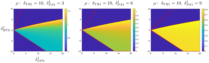
Figure 4: Sensitivity ratios. This series of plots shows the sensitivity ratio $\rho$ as the population 1 policy $(\delta_{SP0}^{1},\delta_{RT0}^{1})$ varies. The red lines indicate the boundaries of the set of feasible policies for population 1. In all plots, we observe the ratio is highest near the curve $C(\delta_{SP0}^{1})$ (dashed red line), i.e. $u_{s}$ becomes effective, and indeed can be more effective than $u_{r}$ for lower values of $\delta_{PS1}^{1}$ (left and center plots). However, $u_{s}$ is generally not as effective relative to $u_{r}$. For higher values of $\delta_{PS1}^{1}$, $u_{s}$ will never be as effective as $u_{r}$, i.e. $\rho<1$ for all policies (right plot). For all simulations, the parameter values are: $\delta_{TR1}=10$, $\theta_{1}=0.75$, $\alpha_{1}=1$, $\epsilon=0.1$.

Throughout the Appendix, we make use of the following notations. The payoff difference function $g_{i}(x_{i},n)$ ($i=1,2$) is bilinear in its two arguments, which we can write as

$$g_{i}(x_{i},n)=a_{i}x_{i}n+b_{i}x_{i}+c_{i}n+d_{i}$$

where we define

$$a_{i} :=\delta_{SP0}^{i}-\delta_{RT0}^{i}+\delta_{PS1}^{i}-\delta_{TR1}^{i}$$ (19)

$$b_{i} :=\delta_{RT0}^{i}-\delta_{SP0}^{i}$$

$$c_{i} :=-(\delta_{PS1}^{i}+\delta_{SP0}^{i})$$

$$d_{i} :=\delta_{SP0}^{i}.$$

Consequently, we can write $\frac{\partial g_{i}}{\partial n}(x_{i})=a_{i}x_{i}+c_{i}<0$ (Assumption 2) and $\frac{\partial g_{i}}{\partial x_{i}}(n)=a_{i}n+b_{i}$. Moreover, we will make use of the variable

$$Y:=b_{1}c_{1}-a_{1}d_{1}=\delta_{TR1}^{1}\delta_{SP0}^{1}-\delta_{RT0}^{1}\delta_{PS1}^{1}$$ (20)

which is positive if and only if $\delta_{RT0}^{1}<\frac{\delta_{TR1}}{\delta_{PS1}}\delta_{SP0}^{1}$, and zero if it holds with equality.

-A Analysis of dynamical system

To establish stability properties of system (7), we need to analyze its Jacobian matrix, which we compute below:

$$J(\boldsymbol{z}):=\begin{bmatrix}J_{11}&0&J_{13}\\ 0&J_{22}&J_{23}\\ \epsilon J_{31}&\epsilon J_{32}&\epsilon J_{33}\\ \end{bmatrix}$$ (21)

for any $\boldsymbol{z}\in[0,1]^{3}$, where

$$J_{11} =x_{1}(1-x_{1})\frac{\partial g_{1}}{\partial x_{1}}(n)+(1-2x_{1})g_{1}(x_{1},n)$$

$$J_{13} =x_{1}(1-x_{1})\frac{\partial g_{1}}{\partial n}(x_{1})$$

$$J_{22} =x_{2}(1-x_{2})\frac{\partial g_{2}}{\partial x_{2}}(n)+(1-2x_{2})g_{2}(x_{2},n)$$

$$J_{23} =x_{2}(1-x_{2})\frac{\partial g_{2}}{\partial n}(x_{2})$$

$$J_{31} =n(1-n)(\theta_{1}+\alpha_{1})$$

$$J_{32} =n(1-n)(\theta_{2}+\alpha_{2})$$

$$J_{33} =(1-2n)(\theta_{1}x_{1}+\theta_{2}x_{2}-\alpha_{1}(1-x_{1})-\alpha_{2}(1-x_{2}))$$

By Assumption 3, no fixed point with $x_{2}>0$ can be stable because $g_{2}(x_{2},n)<0$ for all $x_{2},n$. Hence, we only need to analyze stability properties of fixed points of the form $(x_{1},0,n)$.

Proof of Theorem 3.1.

We first observe that by Assumption 3, it must be the case that $x_{2}(t)\rightarrow 0$ because $g_{2}(x_{2},n)<0$ for all $x_{2},n$. In other words, for any $\varepsilon>0$ and for any initial condition in $(0,1)^{3}$, there is some finite time $t_{\varepsilon}>0$ such that $x_{2}(t)<\varepsilon$ for all $t\geq t_{\varepsilon}$.

(1) $\underline{\alpha_{2}>\theta_{1}}$. We can analyze the limiting behavior by considering the function $V(\boldsymbol{z}):=n$ defined for $\boldsymbol{z}\in[0,1]\times[0,\varepsilon]\times[0,1]$. Its time derivative is simply $\dot{n}=n(1-n)(_{1}(\theta_{1}+\alpha_{1})-(\alpha_{1}+\alpha_{2}))$ (here, we neglect $\varepsilon$ since it is arbitrarily small). Thus, $\dot{V}<0$ for any $x_{1}\in(0,1)$. By LaSalle’s invariance principle, the set $n=0$ is globally asymptotically stable.

(2) $\underline{\alpha_{2}\leq\theta_{1}}$.

The fixed point of the form $(x_{1},0,n)$ with $x_{1},n\in(0,1)$ is determined to be $x_{1}=\frac{\alpha_{1}+\alpha_{2}}{\alpha_{1}+\theta_{1}}$ (from $h(x_{1},n)=0$) and $n=-\frac{b_{1}x_{1}+d_{1}}{a_{1}x_{1}+c_{1}}$ (from $g_{1}(x_{1},n)=0$). It holds that $n\in(0,1)$ if and only if $\frac{\alpha_{2}-\theta_{1}}{\alpha_{1}+\alpha_{2}}\delta_{SP0}^{1}\leq\delta_{RT0}^{1}$. The eigenvalues of $J$ at this point are given by

$$\lambda_{1}=-(\delta_{PS1}^{1}+\delta_{SP0}^{1})n+\delta_{SP0}^{2}<0$$

and

$$\lambda_{2,3} =\frac{1}{2}\left[\frac{}{}(a_{1}n+b_{1})x_{1}(1-x_{1})\pm\right.$$

$$\left.\sqrt{(a_{1}n+b_{1})^{2}x_{1}^{2}(1-x_{1})^{2}-4\epsilon K}\right]$$

where we denote

$$K=n(1-n)(\theta_{1}+\alpha_{1})x_{1}(1-x_{1})|\frac{\partial g_{1}}{\partial n}(x_{1})|>0.$$

The sign of the real parts of $\lambda_{2,3}$ is thus given by the sign of $a_{1}n+b_{1}=\frac{-Y}{|\frac{\partial g_{1}}{\partial n}(x_{1})|}<0$.

The fixed point of the form $(x_{1},0,0)$ with $x_{1}\in(0,1)$ is determined to be $x_{1}=\frac{\delta_{SP0}^{1}}{\delta_{SP0}^{1}-\delta_{RT0}^{1}}$ (from $g_{1}(x_{1},0)=0$). This implies $\delta_{RT0}^{1}<0$. The eigenvalues of $J$ at this point are $\{x_{1}(1-x_{1})b_{1},\delta_{SP0}^{2},\epsilon(x_{1}(\theta_{1}+\alpha_{1})-(\alpha_{1}+\alpha_{2}))\}$. The first and second are negative, and the third is also negative if and only if $\frac{\alpha_{2}-\theta_{1}}{\alpha_{1}+\alpha_{2}}\delta_{SP0}^{1}>\delta_{RT0}^{1}$.

We now verify that all other fixed points cannot be attractive. To see why, we can split the $(x_{1},n)$ plane into four disjoint sectors:

$$Q_{1} :=\{(x_{1},n):x_{1}>\frac{\alpha_{1}+\alpha_{2}}{\alpha_{1}+\theta_{1}},n<\frac{b_{1}x_{1}+d_{1}}{-(a_{1}x_{1}+c_{1})}\}$$ (22)

$$Q_{2} :=\{(x_{1},n):x_{1}>\frac{\alpha_{1}+\alpha_{2}}{\alpha_{1}+\theta_{1}},n\geq\frac{b_{1}x_{1}+d_{1}}{-(a_{1}x_{1}+c_{1})}\}$$

$$Q_{3} :=\{(x_{1},n):x_{1}\leq\frac{\alpha_{1}+\alpha_{2}}{\alpha_{1}+\theta_{1}},n\geq\frac{b_{1}x_{1}+d_{1}}{-(a_{1}x_{1}+c_{1})}\}$$

$$Q_{4} :=\{(x_{1},n):x_{1}\leq\frac{\alpha_{1}+\alpha_{2}}{\alpha_{1}+\theta_{1}},n<\frac{b_{1}x_{1}+d_{1}}{-(a_{1}x_{1}+c_{1})}\}$$

The vector field of the dynamics satisfy $\dot{x}_{1},\dot{n}>0$ in $Q_{1}$, $\dot{x}_{1}\leq 0,\dot{n}>0$ in $Q_{2}$, $\dot{x}_{1}\leq 0,\dot{n}\leq 0$ in $Q_{3}$, and $\dot{x}_{1}>0,\dot{n}\leq 0$ in $Q_{4}$. The equalities hold only on the shared boundaries between the sectors. The unique interior fixed point lies at the single point of intersection of all four sectors. Moreover, we also observe that no point on the borders of $[0,1]^{2}$ can be attractive, since the vector field is oriented such that none of the four quadrants are positively invariant. This establishes the claim. ∎

-B Analysis of optimal consumption

The proof of Theorem 4.1 relies on establishing certain properties about the utility function $U(\alpha_{2})$. Let us define the support of $U$ as

$$\text{supp }U:=\{\alpha_{2}\geq 0:U(\alpha_{2})>0\}.$$ (23)

Throughout the proof, we will use the shorthand notations

$$\bar{\alpha}_{1}:=\frac{\alpha_{1}}{\alpha_{1}+\theta_{1}},\quad\bar{\alpha}_{2}:=\frac{\alpha_{2}}{\alpha_{1}+\theta_{1}}$$ (24)

Proof of Theorem 4.1.

First, we notice that $U(\alpha_{2})=0$ for all $\alpha_{2}>\theta_{1}$, so $U(\alpha_{2})>0$ only if $\alpha_{2}\leq\theta_{1}$. The support of $U$ is the interval $[0,\theta_{1}]$ in the case that $\delta_{RT0}^{1}>0$, and is the interval $[0,\frac{\delta_{SP0}^{1}}{\delta_{SP0}^{1}-\delta_{RT0}^{1}}\theta_{1}+\frac{\delta_{RT0}^{1}}{\delta_{SP0}^{1}-\delta_{RT0}^{1}}\alpha_{1}]$ in the case that $\frac{-\theta_{1}}{\alpha_{1}}\delta_{SP0}^{1}\leq\delta_{RT0}^{1}\leq 0$. At any point in the support, the first derivative of $U$ is

$$U^{\prime}(\alpha_{2}) =R(\alpha_{2})+\alpha_{2}\frac{\partial R}{\partial\alpha_{2}}$$ (25)

$$=R(\alpha_{2})-\alpha_{2}\frac{Y}{(\alpha_{1}+\theta_{1})(\frac{\partial g_{1}}{\partial n}(\bar{\alpha}_{1}+\bar{\alpha}_{2}))^{2}}$$

$$=\frac{b_{1}(\bar{\alpha}_{1}+\bar{\alpha}_{2})+d_{1}}{-(a_{1}(\bar{\alpha}_{1}+\bar{\alpha}_{2})+c_{1})}-\bar{\alpha}_{2}\frac{Y}{(a_{1}(\bar{\alpha}_{1}+\bar{\alpha}_{2})+c_{1})^{2}}$$

We note that $Y\geq 0$ is equivalent to $\delta_{RT0}^{1}\leq\frac{\delta_{TR1}^{1}}{\delta_{PS1}^{1}}\delta_{SP0}^{1}$. Evaluating the second derivative, we obtain

$$U^{\prime\prime}(\alpha_{2}) =-2\frac{Y}{(\alpha_{1}+\theta_{1})(\frac{\partial g_{1}}{\partial n}(\bar{\alpha}_{1}+\bar{\alpha}_{2}))^{2}}$$

$$\quad+\frac{\alpha_{2}Y}{(\alpha_{1}+\theta_{1})}\frac{(-2a_{1})}{(\frac{\partial g_{1}}{\partial n}(\bar{\alpha}_{1}+\bar{\alpha}_{2}))^{3}}$$

$$\propto-\left(1+\frac{\alpha_{2}}{\alpha_{1}+\theta_{1}}\frac{a_{1}}{|\frac{\partial g_{1}}{\partial n}(\bar{\alpha}_{1}+\bar{\alpha}_{2})|}\right)$$

The sign of $U^{\prime\prime}$ then depends only on the factor in parentheses. This factor is monotonic in $\alpha_{2}\in\text{supp }U$. Indeed, the sign of its derivative is the sign of ${-a_{1}^{2}\bar{\alpha}_{1}-a_{1}c_{1}}$, which is independent of $\alpha_{2}$. If it is positive, then $U^{\prime\prime}<0\ \forall\alpha_{2}\in\text{supp }U$. If it is negative, we need to verify that $1+(1-\bar{\alpha}_{1})\frac{a_{1}}{|\frac{\partial g_{1}}{\partial n}(1)|}>0$. Indeed, this is equivalent to the inequality

$$(1-\bar{\alpha}_{1})\frac{\delta_{SP0}^{1}+\delta_{PS1}}{\delta_{RT0}^{1}+\delta_{TR1}}>-\bar{\alpha}_{1}$$ (26)

This is always satisfied because the LHS is positive due to Assumption 2 ($\delta_{RT0}^{1}>-\delta_{TR1}$), and the RHS is negative. This establishes concavity of $U$ in its interval of support.

(a) In this sub-regime, $\text{supp }U=[0,\theta_{1}]$. We need to establish that $U$ is strictly increasing. Since we know that $U^{\prime}(0)=R(0)>0$ and $U$ is concave, we just need to verify $U^{\prime}(\theta_{1})\geq 0$. We have

$$U^{\prime}(\theta_{1}) =R(\theta_{1})-(1-\bar{\alpha}_{1})\frac{Y}{\frac{\partial g_{1}}{\partial n}(1)^{2}}$$

$$=\frac{b_{1}+d_{1}}{-(a_{1}+c_{1})}-(1-\bar{\alpha}_{1})\frac{Y}{(a_{1}+c_{1})^{2}}$$

Multiplying by $(a_{1}+c_{1})^{2}$, we have $U^{\prime}(\theta_{1})\geq 0$ if and only if

$$(\delta_{RT0}^{1})^{2}+((1-\bar{\alpha}_{1})\delta_{PS1}+\delta_{TR1})\delta_{RT0}^{1}$$

$$\quad-(1-\bar{\alpha}_{1})\delta_{TR1}\delta_{SP0}^{1}\geq 0$$

Observe the LHS above is quadratic in $\delta_{RT0}^{1}$, and has a negative and a positive root. Since we are considering $\delta_{RT0}^{1}>0$ in this regime, the condition above is satisfied if and only if $\delta_{RT0}^{1}$ is greater than the positive root, i.e.

$$\delta_{RT0}^{1}\geq C(\delta_{SP0}^{1})$$

(b) Case 1: First we consider $0<\delta_{RT0}^{1}<C(\delta_{SP0}^{1})$. This implies $\text{supp }U=[0,\theta_{1}]$ and $U^{\prime}(\theta_{1})<0$. Therefore, $U(\alpha_{2})$ attains its maximum for some $\alpha_{2}^{*}\in(0,\theta_{1})$. To find $\alpha_{2}^{*}$, we need to solve $U^{\prime}(\alpha_{2})=0$, which yields the quadratic equation

$$-a_{1}b_{1}\bar{\alpha}_{2}^{2}-2b_{1}\frac{\partial g_{1}}{\partial n}(\bar{\alpha}_{1})\bar{\alpha}_{2}+g_{1}(\bar{\alpha}_{1})\frac{\partial g_{1}}{\partial n}(\bar{\alpha}_{1})=0$$ (27)

The “minus” solution is given by

$$\alpha_{2}^{*} =\frac{\theta_{1}+\alpha_{1}}{-a_{1}b_{1}}\left[b_{1}\frac{\partial g_{1}}{\partial n}(\bar{\alpha}_{1})-\right.$$

$$\quad\left.\sqrt{b_{1}^{2}\frac{\partial g_{1}}{\partial n}(\bar{\alpha}_{1})^{2}-a_{1}b_{1}g_{1}(\bar{\alpha}_{1},0)\frac{\partial g_{1}}{\partial n}(\bar{\alpha}_{1})}\right]$$

which reduces to $\alpha_{2}^{*}$ in the Lemma statement. We deduce the “minus” solution must correspond to the critical point by showing it is positive. The sign of $1-\sqrt{\frac{Y}{b_{1}\frac{\partial g_{1}}{\partial n}(\bar{\alpha}_{1})}}$ coincides with the sign of $a_{1}$:

$$1-\sqrt{\frac{Y}{b_{1}\frac{\partial g_{1}}{\partial n}(\bar{\alpha}_{1})}}<0\iff a_{1}(b_{1}\bar{\alpha}_{1}+d_{1})<0$$

Observe $b_{1}\bar{\alpha}_{1}+d_{1}=g_{1}(\bar{\alpha}_{1},0)>0$ since $\delta_{SP0}^{1},\delta_{RT0}^{1}>0$, and therefore $\alpha_{2}^{*}$ is positive. On the other hand, the “plus” solution is negative since the sign of $1+\sqrt{\frac{Y}{b_{1}\frac{\partial g_{1}}{\partial n}(\bar{\alpha}_{1})}}$ is the opposite of $a_{1}$.

Case 2: For $\frac{-\theta_{1}}{\alpha_{1}}\delta_{SP0}^{1}\leq\delta_{RT0}^{1}\leq 0$, $\text{supp }U=[0,\frac{\delta_{SP0}^{1}}{\delta_{SP0}^{1}-\delta_{RT0}^{1}}\theta_{1}+\frac{\delta_{RT0}^{1}}{\delta_{SP0}^{1}-\delta_{RT0}^{1}}\alpha_{1}]$. We can express the utility as

$$U(\alpha_{2})=\alpha_{2}\cdot\begin{cases}-\frac{(\delta_{RT0}^{1}-\delta_{SP0}^{1})({\bar{\alpha}}_{1}+{\bar{\alpha}}_{2})+\delta_{SP0}^{1}}{a_{1}({\bar{\alpha}}_{1}+{\bar{\alpha}}_{2})+c_{1}},&\text{if }\alpha_{2}\in\text{supp }U\\ 0,&\text{else }\end{cases}$$

It holds that $U^{\prime}(0)>0$, $U^{\prime}(\frac{\delta_{SP0}^{1}}{\delta_{SP0}^{1}-\delta_{RT0}^{1}}\theta_{1}+\frac{\delta_{RT0}^{1}}{\delta_{SP0}^{1}-\delta_{RT0}^{1}}\alpha_{1})<0$. Since $U$ is concave, it must attain its maximum in the interval $\alpha_{2}\in(0,\frac{\delta_{SP0}^{1}}{\delta_{SP0}^{1}-\delta_{RT0}^{1}}\theta_{1}+\frac{\delta_{RT0}^{1}}{\delta_{SP0}^{1}-\delta_{RT0}^{1}}\alpha_{1})$. The expression for this point is identical to $\alpha_{2}^{*}$ from Case 1 due to similar arguments. ∎

References

• [1] E. Ostrom, Governing the commons: The evolution of institutions for collective action.   Cambridge university press, 1990.
• [2] J. S. Weitz, C. Eksin, K. Paarporn, S. P. Brown, and W. C. Ratcliff, “An oscillating tragedy of the commons in replicator dynamics with game-environment feedback,” Proceedings of the National Academy of Sciences, vol. 113, no. 47, pp. E7518–E7525, 2016.
• [3] A. R. Tilman, J. B. Plotkin, and E. Akçay, “Evolutionary games with environmental feedbacks,” Nature communications, vol. 11, no. 1, p. 915, 2020.
• [4] L. Gong, W. Yao, J. Gao, and M. Cao, “Limit cycles analysis and control of evolutionary game dynamics with environmental feedback,” Automatica, vol. 145, p. 110536, 2022.
• [5] X. Chen and A. Szolnoki, “Punishment and inspection for governing the commons in a feedback-evolving game,” PLoS computational biology, vol. 14, no. 7, p. e1006347, 2018.
• [6] K. Paarporn, C. Eksin, J. S. Weitz, and Y. Wardi, “Optimal control policies for evolutionary dynamics with environmental feedback,” in 2018 IEEE conference on decision and control (CDC).   IEEE, 2018, pp. 1905–1910.
• [7] X. Wang, Z. Zheng, and F. Fu, “Steering eco-evolutionary game dynamics with manifold control,” Proceedings of the Royal Society A, vol. 476, no. 2233, p. 20190643, 2020.
• [8] A. Satapathi, N. K. Dhar, A. R. Hota, and V. Srivastava, “Coupled evolutionary behavioral and disease dynamics under reinfection risk,” IEEE Transactions on Control of Network Systems, 2023.
• [9] K. Frieswijk, L. Zino, M. Cao, and A. Morse, “Modeling the co-evolution of climate impact and population behavior: A mean-field analysis,” IFAC-PapersOnLine, vol. 56, no. 2, pp. 7381–7386, 2023.
• [10] H. Khazaei, K. Paarporn, A. Garcia, and C. Eksin, “Disease spread coupled with evolutionary social distancing dynamics can lead to growing oscillations,” in 2021 60th IEEE Conference on Decision and Control (CDC).   IEEE, 2021, pp. 4280–4286.
• [11] M. R. Arefin and J. Tanimoto, “Imitation and aspiration dynamics bring different evolutionary outcomes in feedback-evolving games,” Proceedings of the Royal Society A, vol. 477, no. 2251, p. 20210240, 2021.
• [12] L. Stella and D. Bauso, “The impact of irrational behaviors in the optional prisoner’s dilemma with game-environment feedback,” International Journal of Robust and Nonlinear Control, 2021.
• [13] L. Stella, W. Baar, and D. Bauso, “Lower network degrees promote cooperation in the prisoner’s dilemma with environmental feedback,” IEEE Control Systems Letters, vol. 6, pp. 2725–2730, 2022.
• [14] Y. Kawano, L. Gong, B. D. Anderson, and M. Cao, “Evolutionary dynamics of two communities under environmental feedback,” IEEE Control Systems Letters, vol. 3, no. 2, pp. 254–259, 2018.
• [15] A. Govaert, L. Zino, and E. Tegling, “Population games on dynamic community networks,” IEEE Control Systems Letters, vol. 6, pp. 2695–2700, 2022.
• [16] J. Certório, R. J. La, and N. C. Martins, “Epidemic population games for policy design: two populations with viral reservoir case study,” in 2023 62nd IEEE Conference on Decision and Control (CDC).   IEEE, 2023, pp. 7667–7674.
• [17] G. Hardin, “The tragedy of the commons,” Science, vol. 162, no. 3859, pp. 1243–1248, 1968.