Random Pareto front surfaces

Abstract

The Pareto front of a set of vectors is the subset which is comprised solely of all of the best trade-off points. By interpolating this subset, we obtain the optimal trade-off surface. In this work, we prove a very useful result which states that all Pareto front surfaces can be explicitly parametrised using polar coordinates. In particular, our polar parametrisation result tells us that we can fully characterise any Pareto front surface using the length function, which is a scalar-valued function that returns the projected length along any positive radial direction. Consequently, by exploiting this representation, we show how it is possible to generalise many useful concepts from linear algebra, probability and statistics, and decision theory to function over the space of Pareto front surfaces. Notably, we focus our attention on the stochastic setting where the Pareto front surface itself is a stochastic process. Among other things, we showcase how it is possible to define and estimate many statistical quantities of interest such as the expectation, covariance and quantile of any Pareto front surface distribution. As a motivating example, we investigate how these statistics can be used within a design of experiments setting, where the goal is to both infer and use the Pareto front surface distribution in order to make effective decisions. Besides this, we also illustrate how these Pareto front ideas can be used within the context of extreme value theory. Finally, as a numerical example, we applied some of our new methodology on a real-world air pollution data set.

1 Introduction

The Pareto front is often regarded as the natural generalisation of the maximum (or minimum) for vector-valued sets. This generalisation is based on the Pareto partial ordering relation, which gives us a way to compare between any two vectors when possible. Geometrically, the Pareto front can be used to define a surface in the vector space which describes the best possible trade-offs one can obtain between the different components. The primary focus of this work will be to study this space of Pareto front surfaces in more detail. To accomplish this, we establish our main result in Theorem 3.1, which gives us an explicit way to parametrise any Pareto front surface using polar coordinates. The rest of the work is then focussed on using this polar parametrisation result in order to generalise existing concepts from linear algebra, probability and statistics, and decision theory to function over this exotic space of Pareto front surfaces. In particular, we focus our attention on the stochastic setting where the Pareto front surface itself is random. Under this regime, our polar parametrisation result tells us that we can treat any random Pareto front surface as an infinite-dimensional stochastic process (10), which is indexed by the set of positive unit vectors. This stochastic process can then be used along with standard ideas from functional data analysis in order to define and estimate any Pareto front surface statistic of interest in a principled and efficient manner—more details in Section 4. We then proceed to show how these ideas can be used within a standard decision making workflow, where one is interested in actively identifying decisions which lead to the best trade-off for the decision maker—see Section 5.1 and Section 5.2. As another independent application, we also highlight how our work on random Pareto front surfaces can be applied within the domain of multivariate extreme value theory—more details in Section 5.3. Lastly, in Section 5.4, we present a numerical example which demonstrates how our ideas can be used in order to analyse Pareto fronts in time series data. Precisely, we focus our attention on the change in the maximum amount of daily air pollution in North Kensington, London. We find that the daily Pareto front of pollutant levels has indeed been reduced after the introduction of many recent pollution reduction initiatives.

1.1 Structure of the paper

The remainder of the paper is organised as follows: In Section 2, we introduce the key definitions and nomenclature that will be used throughout the paper. In Section 3, we present our main result, which gives an explicit parametrisation of any Pareto front surface based on polar coordinates. We then use this polar parametrisation in order to define some useful operations and concepts on the space of Pareto front surfaces. Notably we define the concept of an order-preserving transformation (Section 3.1), a length-based utility function (Section 3.2) and a length-based loss function (Section 3.3). In Section 4, we study the setting where the Pareto front surface is random and define many useful statistics of interest such as the expectation (Section 4.1), covariance (Section 4.2) and quantiles (Section 4.3), among others. We also connected our discussion with existing work on Pareto front surface distributions, which are based solely on ideas from random set theory (Section 4.6). In Section 5, we demonstrate the effectiveness of these new ideas on some practical applications. For instance, in Section 5.1, we present a novel visualisation strategy based our polar parametrisation result. In particular, we show how it is possible to construct a picture of the whole Pareto front surface by using a family of low-dimensional slices. Consequently, in Section 5.2, we illustrate how all of these uncertainty quantification and visualisation ideas can be used within a standard Bayesian experimental design setting. Specifically, we demonstrate how these tools can be used both during an optimisation routine (Section 5.2.1) and also in the post-decision setting (Section 5.2.2). The former stage focusses on the problem of identifying the best experiments to run, whilst the latter stage is focussed on identifying the inputs which are most likely going lead to the desired outputs. Subsequently, in Section 5.3, we demonstrate how it is possible to adapt some prominent results from extreme value theory to work in the multivariate setting, where the maximum is defined using the Pareto partial ordering. This is in contrast to most existing work in multivariate extreme value theory, which has largely focussed on the setting where the vector-valued maximum is defined in a component-wise fashion. Afterwards, in Section 5.4, we present a case study on how some of these Pareto front ideas can be used in order to quantify changes in the daily maximum air pollutant levels in a part of west London. In Section 6, we conclude this work and include a discussion on future research directions. Finally, in Appendix A, we include the proofs of all of the results that are stated within the paper. The code that is needed to reproduce the figures and numerical experiments are available in our Github repository: https://github.com/benmltu/scalarize.

2 Preliminaries

In this work, we study the properties of Pareto front surfaces, which are the surfaces obtained by interpolating the Pareto optimum of a vector-valued set. Without loss of generality, we assume throughout that the goal of interest is maximisation. Naturally, the minimisation problem can also be treated by simply negating the corresponding set of vectors. Note that there are many subtle differences in the literature when it comes to defining a Pareto front surface. For this reason, we will now carefully define the concept of the truncated interpolated weak Pareto front, which will be the primary focus of this work.

Definition 2.1 (Pareto domination)

The weak, strict and strong Pareto domination is denoted by the binary relations $\succeq,\succ$ and $\succ\mathrel{\mkern-5.0mu}\succ$, respectively. We say a vector $\mathbf{y}\in\mathbb{R}^{M}$ weakly, strictly or strongly Pareto dominates another vector $\mathbf{y^{\prime}}\in\mathbb{R}^{M}$ if

$$\mathbf{y}\succeq\mathbf{y^{\prime}} \iff\mathbf{y}-\mathbf{y^{\prime}}\in\mathbb{R}_{\geq 0}^{M},$$

$$\mathbf{y}\succ\mathbf{y^{\prime}} \iff\mathbf{y}-\mathbf{y^{\prime}}\in\mathbb{R}_{\geq 0}^{M}\setminus\{\mathbf{0}_{M}\},$$

$$\mathbf{y}\succ\mathrel{\mkern-5.0mu}\succ\mathbf{y^{\prime}} \iff\mathbf{y}-\mathbf{y^{\prime}}\in\mathbb{R}_{>0}^{M},$$

respectively, where $\mathbf{0}_{M}\in\mathbb{R}^{M}$ denotes the $M$-dimensional vector of zeros.

Definition 2.2 (Domination region)

The Pareto domination region is defined as the collection of points which dominates (or is dominated) by a particular set of vectors $A\subset\mathbb{R}^{M}$, that is

$$\mathbb{D}_{\diamond}[A]:=\cup_{\mathbf{a}\in A}\{\mathbf{y}\in\mathbb{R}^{M}:\mathbf{y}\diamond\mathbf{a}\},$$

where $\diamond\in\{\preceq,\succeq,\prec,\succ,\prec\mathrel{\mkern-5.0mu}\prec,\succ\mathrel{\mkern-5.0mu}\succ\}$ denotes a partial ordering relation. In addition, we denote the truncated domination region by $\mathbb{D}_{\diamond,\boldsymbol{\eta}}[A]:=\mathbb{D}_{\diamond}[A]\cap\mathbb{D}_{\succ\mathrel{\mkern-5.0mu}\succ}[\{\boldsymbol{\eta}\}]$, for any reference vector $\boldsymbol{\eta}\in\mathbb{R}^{M}$ and denote the complement of any domination region by $\mathbb{D}^{C}_{\diamond}[A]:=\mathbb{R}^{M}\setminus\mathbb{D}_{\diamond}[A]$.

Definition 2.3 (Pareto optimality)

Given a bounded set of vectors $A\subset\mathbb{R}^{M}$, a point $\mathbf{a}\in A$ is weakly or strictly Pareto optimal if there does not exist another vector $\mathbf{a}^{\prime}\in A$ which strongly or strictly Pareto dominates it, respectively. The collection of all weakly or strictly Pareto optimal vectors in this set is called the weak or strict Pareto front, $\mathcal{Y}^{\textnormal{weak}}[A]:=A\cap\mathbb{D}^{C}_{\prec\mathrel{\mkern-5.0mu}\prec}[A]$ and $\mathcal{Y}^{\textnormal{strict}}[A]:=A\cap\mathbb{D}^{C}_{\prec}[A]$, respectively.

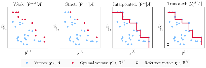
Figure 1: An illustration of the different Pareto fronts in $M=2$ dimensions.

Although strict Pareto optimality is a desirable quality, it is a difficult operation to work with because it returns a subset of the original set, which could contain an arbitrary number of points. To address this problem, we consider working with a more relaxed notion of Pareto optimality, which we refer to as the interpolated weak Pareto optimality (Definition 2.4). Conceptually, we define the interpolated weak Pareto front as the interpolation of the strict Pareto front. This interpolation defines a surface in the $M$-dimensional vector space. For practical convenience, we also define the truncated interpolated weak Pareto front, which truncates this surface at some reference point $\boldsymbol{\eta}\in\mathbb{R}^{M}$—see Figure 1 for an illustration.

Definition 2.4 (Interpolated weak optimality)

Given a bounded set of vectors $A\subset\mathbb{R}^{M}$, we define the interpolated weak Pareto front as the weak Pareto front of its weak domination region after closure, that is: $\mathcal{Y}^{\textnormal{int}}[A]:=\mathcal{Y}^{\textnormal{weak}}[\mathbb{D}_{\preceq}[\textsc{Closure}(A)]]$. By truncating this surface at some reference vector $\boldsymbol{\eta}\in\mathbb{R}^{M}$, we obtain the truncated interpolated weak Pareto front $\mathcal{Y}_{\boldsymbol{\eta}}^{\textnormal{int}}[A]:=\mathcal{Y}^{\textnormal{int}}[A]\cap\mathbb{D}_{\succ\mathrel{\mkern-5.0mu}\succ}[\{\boldsymbol{\eta}\}]$. We denote the set of all possible non-empty truncated interpolated weak Pareto fronts by $\mathbb{Y}^{*}_{\boldsymbol{\eta}}\subset 2^{\mathbb{R}^{M}}$.

In practice, the set of objective vectors that we seek to optimise is often the output of some vector-valued objective function $g:\mathbb{X}\rightarrow\mathbb{R}^{M}$, where $\mathbb{X}$ denotes the space of feasible inputs. In this setting, the optimal set of objectives is given by the Pareto front of the feasible objective vectors. For example, the strict Pareto front is given by the set $\mathcal{Y}^{\textnormal{strict}}[\{g(\mathbf{x})\}_{\mathbf{x}\in\mathbb{X}}]\subset\mathbb{R}^{M}$, whilst the strict Pareto set is defined as the corresponding pre-image. Similarly, we can also define the other weak variants of the Pareto front and Pareto set as well.

Remark 2.1 (Reference vector)

Throughout this work, we will assume that the reference vector $\boldsymbol{\eta}\in\mathbb{R}^{M}$ is known and fixed by the decision maker. Intuitively, this parameter is just used as a way to lower bound the set of vectors that we are interested in targetting. In the multi-objective literature, it is common to see this vector set to an estimate that is equal or close the nadir point, which is the vector comprised of the worst possible values for each objective: $\eta^{(m)}=\min_{\mathbf{x}\in\mathbb{X}}g^{(m)}(\mathbf{x})$ for objectives $m=1,\dots,M$. In fact, some authors have suggested using a reference point that is slightly worse than the nadir when we are interested in evaluating the performance of a multi-objective algorithm (Ishibuchi et al., 2017).

Nomenclature

For convenience, unless otherwise stated, we will from now on refer to a set as being a Pareto front or Pareto front surface if it is a truncated interpolated weak Pareto front (Definition 2.4). We will refer to a point as being Pareto optimal if it lies on this truncated interpolated weak Pareto front. In addition, we will refer to the set of all non-empty truncated interpolated weak Pareto front $\mathbb{Y}^{*}_{\boldsymbol{\eta}}$ as the set of all Pareto fronts or Pareto front surfaces.

3 Polar parametrisation

We now present the main result of this paper (Theorem 3.1), which states that all non-empty Pareto front surfaces are isomorphic to the set of positive unit vectors

$$\mathcal{S}^{M-1}_{+}:=\{\mathbf{z}\in\mathbb{R}_{>0}^{M}:||\mathbf{z}||_{L^{2}}=1\}\in\mathbb{Y}^{*}_{\mathbf{0}_{M}}.$$

Notably we present an explicit representation for this isomorphism in (5), which we refer to as the polar parametrisation of a Pareto front surface. The name of this representation is motivated by the fact that we rely on the hyperspherical polar coordinates transformation in order to derive this result. The intuitive idea behind this result is concisely described in Figure 2. Informally speaking, we can identify each Pareto optimal point by drawing a line from the reference vector $\boldsymbol{\eta}\in\mathbb{R}^{M}$ along a positive direction $\boldsymbol{\lambda}\in\mathcal{S}^{M-1}_{+}$. If we know the length of these lines $\ell_{\boldsymbol{\eta},\boldsymbol{\lambda}}\in\mathbb{R}$ when it intersects the Pareto front surface, then we can reconstruct the Pareto front surface by using a linear mapping: $\boldsymbol{\eta}+\ell_{\boldsymbol{\eta},\boldsymbol{\lambda}}\boldsymbol{\lambda}\in\mathbb{R}^{M}$ for $\boldsymbol{\lambda}\in\mathcal{S}^{M-1}_{+}$. In the following paragraphs, we will formalise this idea more concretely and give an explicit construction for this length function.

Polar coordinates

To prove Theorem 3.1, we rely on the following coordinate system transformation $\mathcal{T}_{\boldsymbol{\eta}}:\mathbb{D}_{\succ\mathrel{\mkern-5.0mu}\succ}[\{\boldsymbol{\eta}\}]\rightarrow\mathcal{S}^{M-1}_{+}\times\mathbb{R}_{>0}$,

$$\begin{split}\mathcal{T}_{\boldsymbol{\eta}}(\mathbf{y})&:=(\boldsymbol{\lambda}_{\boldsymbol{\eta}}^{*}(\mathbf{y}),s_{\boldsymbol{\eta},\boldsymbol{\lambda}_{\boldsymbol{\eta}}^{*}(\mathbf{y})}(\mathbf{y}))=\biggl{(}\frac{\mathbf{y}-\boldsymbol{\eta}}{||\mathbf{y}-\boldsymbol{\eta}||_{L^{2}}},||\mathbf{y}-\boldsymbol{\eta}||_{L^{2}}\biggr{)},\end{split}$$ (1)

which maps any vector $\mathbf{y}\in\mathbb{D}_{\succ\mathrel{\mkern-5.0mu}\succ}[\{\boldsymbol{\eta}\}]$ to a positive unit vector $\boldsymbol{\lambda}_{\boldsymbol{\eta}}^{*}(\mathbf{y})\in\mathcal{S}^{M-1}_{+}$ and a positive scalar $s_{\boldsymbol{\eta},\boldsymbol{\lambda}_{\boldsymbol{\eta}}^{*}(\mathbf{y})}(\mathbf{y})>0$. Intuitively, this mapping can be interpreted as a variant of the hyperspherical polar coordinates transformation centred at the reference vector $\boldsymbol{\eta}\in\mathbb{R}^{M}$. In our setting, the positive unit vector plays the role of the angle, whilst the positive scalar plays the role of the projected length. The key difference between this transformation and the standard hyperspherical polar coordinates transformation is that here we restrict our attention to just the angles lying in the positive orthant. These positive directions are the only ones which will lead to a Pareto optimal point. Formally, the coordinate transformation in (1) relies on the length scalarisation function $s_{\boldsymbol{\eta},\boldsymbol{\lambda}}:\mathbb{R}^{M}\rightarrow\mathbb{R}$,

$$s_{\boldsymbol{\eta},\boldsymbol{\lambda}}(\mathbf{y}):=\textsc{Length}[L_{\boldsymbol{\eta},\boldsymbol{\lambda}}\cap(\boldsymbol{\eta},\mathbf{y})]=\min_{m=1,\dots,M}\frac{\max(y^{(m)}-\eta^{(m)},0)}{\lambda^{(m)}},$$ (2)

which is a non-negative function that is defined for all vectors $\mathbf{y}\in\mathbb{R}^{M}$. Conceptually, when the objective vector lies in the truncated space $\mathbf{y}\in\mathbb{D}_{\succ\mathrel{\mkern-5.0mu}\succ}[\{\boldsymbol{\eta}\}]$, then the length scalarisation function computes the length of the line $L_{\boldsymbol{\eta},\boldsymbol{\lambda}}:=\{\boldsymbol{\eta}+t\boldsymbol{\lambda}:t\in\mathbb{R}\}$ lying in the open hyper-rectangle $(\boldsymbol{\eta},\mathbf{y}):=\{\mathbf{z}\in\mathbb{R}^{M}:z^{(m)}\in(\eta^{(m)},y^{(m)})\text{ for }m=1,\dots,M\}$—see the left of Figure 4 for an illustration of this intuition in two dimensions. Consequently, the optimal direction function $\boldsymbol{\lambda}_{\boldsymbol{\eta}}^{*}:\mathbb{D}_{\succ\mathrel{\mkern-5.0mu}\succ}[\{\boldsymbol{\eta}\}]\rightarrow\mathcal{S}^{M-1}_{+}$ is the function that returns the largest projected length

$$\boldsymbol{\lambda}_{\boldsymbol{\eta}}^{*}(\mathbf{y}):=\frac{\mathbf{y}-\boldsymbol{\eta}}{||\mathbf{y}-\boldsymbol{\eta}||_{L^{2}}}\in\operatorname*{arg\,max}_{\boldsymbol{\lambda}\in\mathcal{S}_{+}^{M-1}}s_{\boldsymbol{\eta},\boldsymbol{\lambda}}(\mathbf{y})$$ (3)

for any vector $\mathbf{y}\in\mathbb{D}_{\succ\mathrel{\mkern-5.0mu}\succ}[\{\boldsymbol{\eta}\}]$ lying in the truncated space. Note that to invert this coordinate transformation we can simply apply the linear transformation $\mathcal{T}_{\boldsymbol{\eta}}^{-1}:\mathcal{S}^{M-1}_{+}\times\mathbb{R}_{>0}\rightarrow\mathbb{D}_{\succ\mathrel{\mkern-5.0mu}\succ}[\{\boldsymbol{\eta}\}]$, where $\mathcal{T}_{\boldsymbol{\eta}}^{-1}((\boldsymbol{\lambda},l)):=\boldsymbol{\eta}+l\boldsymbol{\lambda}$ for any $(\boldsymbol{\lambda},l)\in\mathcal{S}^{M-1}_{+}\times\mathbb{R}_{>0}$.

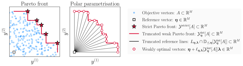
Figure 2: An illustration of the polar parametrisation result in $M=2$ dimensions.

Polar surfaces

By construction, each reference line $L_{\boldsymbol{\eta},\boldsymbol{\lambda}}$ is pointing in an increasing direction. This implies that each reference line should intersect the Pareto front surface in exactly one point if it is non-empty. If this is not the case, then we get a contradiction to Pareto optimality. Using this observation, we define the set of polar surfaces $\mathbb{L}_{\boldsymbol{\eta}}\subset 2^{\mathbb{R}^{M}}$, in Definition 3.1, to be the set of vectors lying in the truncated space which satisfies this intersection constraint.

Definition 3.1 (Polar surfaces)

For any reference vector $\boldsymbol{\eta}\in\mathbb{R}^{M}$, a set $A\subset\mathbb{R}^{M}$ is called a polar surface, $A\in\mathbb{L}_{\boldsymbol{\eta}}$, if and only if the following statement holds:

$$A\in\mathbb{L}_{\boldsymbol{\eta}}\iff A\subset\mathbb{D}_{\succ\mathrel{\mkern-5.0mu}\succ}[\{\boldsymbol{\eta}\}]\cup\{\boldsymbol{\eta}\}\enskip\text{ and }\enskip|A\cap L_{\boldsymbol{\eta},\boldsymbol{\lambda}}|=1\text{ for all }\boldsymbol{\lambda}\in\mathcal{S}^{M-1}_{+}.$$

Moreover, for this set of polar surfaces $\mathbb{L}_{\boldsymbol{\eta}}$, we define the projected length function $\ell_{\boldsymbol{\eta},\boldsymbol{\lambda}}:\mathbb{L}_{\boldsymbol{\eta}}\rightarrow\mathbb{R}_{\geq 0}$ as the function which returns the $L^{2}$-distance of the intersected point along any positive direction $\boldsymbol{\lambda}\in\mathcal{S}^{M-1}_{+}$:

$$\ell_{\boldsymbol{\eta},\boldsymbol{\lambda}}[A]=\max_{\mathbf{a}\in A\cap L_{\boldsymbol{\eta},\boldsymbol{\lambda}}}||\mathbf{a}||_{L^{2}}$$

for any polar surface $A\in\mathbb{L}_{\boldsymbol{\eta}}$.

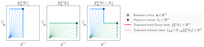
Figure 3: An illustration of the polar parametrisation associated with a set of two points.

Note that there is a duality between a polar surface $A\in\mathbb{L}_{\boldsymbol{\eta}}$ and its projected lengths:

$$A\in\mathbb{L}_{\boldsymbol{\eta}}\longleftrightarrow\{\ell_{\boldsymbol{\eta},\boldsymbol{\lambda}}[A]\geq 0:\boldsymbol{\lambda}\in\mathcal{S}^{M-1}_{+}\}.$$

By design, we can easily reconstruct the whole polar surface $A\in\mathbb{L}_{\boldsymbol{\eta}}$, from its collection of projected lengths, by using the equation

$$A=\{\boldsymbol{\eta}+\ell_{\boldsymbol{\eta},\boldsymbol{\lambda}}[A]\boldsymbol{\lambda}\in\mathbb{R}^{M}:\boldsymbol{\lambda}\in\mathcal{S}_{+}^{M-1}\}.$$ (4)

In other words, we can interpret the set of polar surfaces $\mathbb{L}_{\boldsymbol{\eta}}$ as a set of sets of vectors which can be completely characterised by its projected lengths. Geometrically speaking, any polar surface $A\in\mathbb{L}_{\boldsymbol{\eta}}$ can be obtained by translating and then stretching the set of positive unit vectors $\mathcal{S}_{+}^{M-1}$ along the positive radial directions. Our main result in Theorem 3.1 states that the set of all Pareto front surfaces is indeed a special subset of this set: $\mathbb{Y}^{*}_{\boldsymbol{\eta}}\subset\mathbb{L}_{\boldsymbol{\eta}}$. Precisely, it is the subset where the Pareto partial ordering is preserved and the projected length function has an explicit formula given in terms of the length scalarisation function (2). We present the proof of this result in Section A.1 and an illustration of it in Figure 2.

Theorem 3.1 (Polar parametrisation)

For any bounded set of vectors $A\subset\mathbb{R}^{M}$ and reference vector $\boldsymbol{\eta}\in\mathbb{R}^{M}$, if the corresponding Pareto front surface is not empty $\mathcal{Y}_{\boldsymbol{\eta}}^{\textnormal{int}}[A]\neq\emptyset$, then it admits the following polar parametrisation:

$$\mathcal{Y}_{\boldsymbol{\eta}}^{\textnormal{int}}[A]=\biggl{\{}\boldsymbol{\eta}+\sup_{\mathbf{a}\in A}s_{\boldsymbol{\eta},\boldsymbol{\lambda}}(\mathbf{a})\boldsymbol{\lambda}\in\mathbb{R}^{M}:\boldsymbol{\lambda}\in\mathcal{S}_{+}^{M-1}\biggr{\}}$$ (5)

where $\ell_{\boldsymbol{\eta},\boldsymbol{\lambda}}[\mathcal{Y}_{\boldsymbol{\eta}}^{\textnormal{int}}[A]]=\sup_{\mathbf{a}\in A}s_{\boldsymbol{\eta},\boldsymbol{\lambda}}(\mathbf{a})$ is the projected length along $\boldsymbol{\lambda}\in\mathcal{S}_{+}^{M-1}$.

Remark 3.1 (Singleton front)

When the Pareto front surface is empty, $\mathcal{Y}_{\boldsymbol{\eta}}^{\textnormal{int}}[A]=\emptyset$, then the right hand side of (5) evaluates to the degenerate polar surface $\{\boldsymbol{\eta}\}\in\mathbb{L}_{\boldsymbol{\eta}}$. This event can happen when the reference vector $\boldsymbol{\eta}\in\mathbb{R}^{M}$ is set too aggressively in such a way as it weakly dominates the entire feasible objective space.

Remark 3.2 (Conceptual idea)

The explicit form of the polar parametrisation (5) can be derived in an constructive manner. Firstly, one can show that the Pareto front surface of a single point $\mathbf{a}\in\mathbb{D}_{\succ\mathrel{\mkern-5.0mu}\succ}[\{\boldsymbol{\eta}\}]$ can be written as the polar surface

$$\mathcal{Y}_{\boldsymbol{\eta}}^{\textnormal{int}}[\{\mathbf{a}\}]=\{\boldsymbol{\eta}+s_{\boldsymbol{\eta},\boldsymbol{\lambda}}(\mathbf{a})\boldsymbol{\lambda}\in\mathbb{R}^{M}:\boldsymbol{\lambda}\in\mathcal{S}_{+}^{M-1}\}\in\mathbb{L}_{\boldsymbol{\eta}}.$$

Consequently, we can then determine the Pareto front surface of any set of points $A\subset\mathbb{D}_{\succ\mathrel{\mkern-5.0mu}\succ}[\{\boldsymbol{\eta}\}]$ by simply computing the union of the corresponding individual Pareto front surfaces and then removing all the points which are sub-optimal, that is

$$\mathcal{Y}_{\boldsymbol{\eta}}^{\textnormal{int}}[A] =\mathcal{Y}_{\boldsymbol{\eta}}^{\textnormal{int}}[\cup_{\mathbf{a}\in A}\mathcal{Y}_{\boldsymbol{\eta}}^{\textnormal{int}}[\{\mathbf{a}\}]]$$

$$=\mathcal{Y}_{\boldsymbol{\eta}}^{\textnormal{int}}[\{\boldsymbol{\eta}+s_{\boldsymbol{\eta},\boldsymbol{\lambda}}(\mathbf{a})\boldsymbol{\lambda}\in\mathbb{R}^{M}:\mathbf{a}\in A,\boldsymbol{\lambda}\in\mathcal{S}_{+}^{M-1}\}]$$

$$=\biggl{\{}\boldsymbol{\eta}+\sup_{\mathbf{a}\in A}s_{\boldsymbol{\eta},\boldsymbol{\lambda}}(\mathbf{a})\boldsymbol{\lambda}\in\mathbb{R}^{M}:\boldsymbol{\lambda}\in\mathcal{S}_{+}^{M-1}\biggr{\}}.$$

Remarkably, this overall procedure turns out to be equivalent to just retaining the points which achieve the maximal projected lengths along each positive direction $\boldsymbol{\lambda}\in\mathcal{S}^{M-1}_{+}$. An illustration of this conceptual idea is presented in Figure 3. Note however that the proof of the result in Section A.1 does not actually follow this intuitive construction. Instead, our proof is derived in a more technical way by taking advantage of a well-known optimisation result regarding the Chebyshev scalarisation function (Miettinen, 1998, Part 2, Theorem 3.4.5). The primary reason why we take this more general approach is to ensure that our polar parametrisation result holds for sets lying in the whole objective space $\mathbb{R}^{M}$ as opposed to just the truncated objective space $\mathbb{D}_{\succ\mathrel{\mkern-5.0mu}\succ}[\{\boldsymbol{\eta}\}]$.

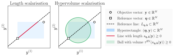
Figure 4: An illustration of the length-based scalarisation functions in $M=2$ dimensions.

Remark 3.3 (Other representations)

The coordinate system transformation that we performed in (1) is appealing because it admits a representation for the Pareto front surface, which is simple, explicit and has a linear dependency on the projected length values. Nevertheless, we can easily obtain other nonlinear representations of a Pareto front surface by taking advantage of transformation functions. For example, let $\tau:\mathbb{R}^{M}\rightarrow\mathbb{R}^{M}$ denote an invertible and strictly monotonically increasing transformation function such that $\mathbf{y}\succeq\mathbf{y}^{\prime}\iff\tau(\mathbf{y})\succeq\tau(\mathbf{y}^{\prime})$ for any $\mathbf{y},\mathbf{y}^{\prime}\in\mathbb{R}^{M}$. Then, by a simple monotonicity argument, we can show that the following parametrisation of the Pareto front surface is also valid:

$$\mathcal{Y}_{\boldsymbol{\eta}}^{\textnormal{int}}[A]=\biggl{\{}\tau^{-1}\Bigl{(}\tau(\boldsymbol{\eta})+\sup_{\mathbf{a}\in A}s_{\tau(\boldsymbol{\eta}),\boldsymbol{\lambda}}(\tau(\mathbf{a}))\boldsymbol{\lambda}\Bigr{)}\in\mathbb{R}^{M}:\boldsymbol{\lambda}\in\mathcal{S}_{+}^{M-1}\biggr{\}}.$$

Intuitively, this reformulation works by performing the polar parametrisation in the transformed space before inverting the result. Note that strict monotonicity is required here because we want the Pareto front surface to be invariant under these transformations: $\mathcal{Y}_{\boldsymbol{\eta}}^{\textnormal{int}}[A]=\tau^{-1}(\mathcal{Y}_{\tau(\boldsymbol{\eta})}^{\textnormal{int}}[\tau(A)])$.

Remark 3.4 (Computational cost)

For a finite set $A\subset\mathbb{R}^{M}$, the worst-case cost involved with computing the strictly Pareto optimal front $\mathcal{Y}^{\textnormal{strict}}[A]\subset\mathbb{R}^{M}$ is $\mathcal{O}(|A|^{2}M)$. In contrast, the worst-case cost involved with computing a finite approximation of the polar parametrised Pareto front surface $\mathcal{Y}_{\boldsymbol{\eta}}^{\textnormal{int}}[A]\subset\mathbb{R}^{M}$ is $\mathcal{O}(|\Lambda||A|M)$, where $\Lambda=\{\boldsymbol{\lambda}_{1},\boldsymbol{\lambda}_{2},\dots\}$ denotes a finite set of positive unit vectors.

3.1 Order-preserving transformations

The polar parametrisation result in Theorem 3.1 tells us that any Pareto front surface is completely defined by its projected lengths. Conceptually, this means that we can define transformations on the space of Pareto front surfaces by simply applying transformations on the projected lengths. As long as these transformation operations preserve the Pareto partial ordering, then we can be assured that resulting set is also a valid Pareto front surface. In Proposition 3.1, we give two necessary and sufficient conditions for this to happen. The first condition (C1) states that the projected lengths have to be positive—this condition ensures that the resulting Pareto front surface is non-empty. The second condition (C2) is the Pareto optimality condition—this ensures that we cannot find two vectors in the set such that one strongly dominates the other. The necessity of this latter condition follows from the spirit of Lemma 3.1, which presents some equivalent statements for Pareto domination based on the length scalarisation function (2). The proof of both of these result are presented in Section A.2 and Section A.3.

Lemma 3.1 (Domination equivalence)

For any Pareto front surface $A^{*}\in\mathbb{Y}_{\boldsymbol{\eta}}^{*}$ and vector $\mathbf{y}\in\mathbb{D}_{\succ\mathrel{\mkern-5.0mu}\succ}[\{\boldsymbol{\eta}\}]$, we have the following equivalences:

$$\mathbf{y}\in\mathbb{D}_{\preceq,\boldsymbol{\eta}}[A^{*}]\iff s_{\boldsymbol{\eta},\boldsymbol{\lambda}_{\boldsymbol{\eta}}^{*}(\mathbf{y})}(\mathbf{y})\leq\ell_{\boldsymbol{\eta},\boldsymbol{\lambda}_{\boldsymbol{\eta}}^{*}(\mathbf{y})}[A^{*}],$$

$$\mathbf{y}\in\mathbb{D}_{\prec\mathrel{\mkern-5.0mu}\prec,\boldsymbol{\eta}}[A^{*}]\iff s_{\boldsymbol{\eta},\boldsymbol{\lambda}_{\boldsymbol{\eta}}^{*}(\mathbf{y})}(\mathbf{y})<\ell_{\boldsymbol{\eta},\boldsymbol{\lambda}_{\boldsymbol{\eta}}^{*}(\mathbf{y})}[A^{*}],$$

$$\mathbf{y}\in\mathbb{D}_{\succ\mathrel{\mkern-5.0mu}\succ,\boldsymbol{\eta}}[A^{*}]\iff s_{\boldsymbol{\eta},\boldsymbol{\lambda}_{\boldsymbol{\eta}}^{*}(\mathbf{y})}(\mathbf{y})>\ell_{\boldsymbol{\eta},\boldsymbol{\lambda}_{\boldsymbol{\eta}}^{*}(\mathbf{y})}[A^{*}],$$

$$\mathbf{y}\in\mathbb{D}_{\succeq,\boldsymbol{\eta}}[A^{*}]\iff s_{\boldsymbol{\eta},\boldsymbol{\lambda}_{\boldsymbol{\eta}}^{*}(\mathbf{y})}(\mathbf{y})\geq\ell_{\boldsymbol{\eta},\boldsymbol{\lambda}_{\boldsymbol{\eta}}^{*}(\mathbf{y})}[A^{*}],$$

where $s_{\boldsymbol{\eta},\boldsymbol{\lambda}_{\boldsymbol{\eta}}^{*}(\mathbf{y})}(\mathbf{y})=||\mathbf{y}-\boldsymbol{\eta}||_{L^{2}}$ and $\ell_{\boldsymbol{\eta},\boldsymbol{\lambda}_{\boldsymbol{\eta}}^{*}(\mathbf{y})}[A^{*}]=\max_{\mathbf{a}\in A^{*}}s_{\boldsymbol{\eta},\boldsymbol{\lambda}_{\boldsymbol{\eta}}^{*}(\mathbf{y})}(\mathbf{a})$.

Proposition 3.1 (Pareto front conditions)

Consider a polar surface $A\in\mathbb{L}_{\boldsymbol{\eta}}$, then this set is a Pareto front surface, $A=\mathcal{Y}_{\boldsymbol{\eta}}^{\textnormal{int}}[A]$, if and only if the following two conditions holds:

1. The positive lengths condition: $\ell_{\boldsymbol{\eta},\boldsymbol{\lambda}}[A]>0$ for all $\boldsymbol{\lambda}\in\mathcal{S}_{+}^{M-1}$.

2. The maximum ratio condition: $\max_{m=1,\dots,M}\frac{\ell_{\boldsymbol{\eta},\boldsymbol{\lambda}}[A]\lambda^{(m)}}{\ell_{\boldsymbol{\eta},\boldsymbol{\upsilon}}[A]\upsilon^{(m)}}\geq 1$ for all $\boldsymbol{\lambda},\boldsymbol{\upsilon}\in\mathcal{S}_{+}^{M-1}$.

Proposition 3.1 gives us two simple conditions on the projected length function which can be easily checked whenever we want to determine whether a Pareto front surface is valid. For convenience, we will say a transformation (or an operation) acting on the space of Pareto front surfaces is order-preserving if the resulting projected length function satisfies the two conditions in Proposition 3.1. Below, we present some notable order-preserving operations which are defined over the general space of polar surfaces. Firstly, we present the union operation in Example 3.1, which formalises the idea described in Remark 3.2.

Example 3.1 (Union)

Consider two Pareto front surfaces $A^{*},B^{*}\in\mathbb{Y}_{\boldsymbol{\eta}}^{*}$, by Theorem 3.1, we can compute the Pareto front surface of the union of these two sets by simply taking the maximum of the projected lengths, that is

$$\mathcal{Y}_{\boldsymbol{\eta}}^{\textnormal{int}}[A^{*}\cup B^{*}]=\{\boldsymbol{\eta}+\max(\ell_{\boldsymbol{\eta},\boldsymbol{\lambda}}[A^{*}],\ell_{\boldsymbol{\eta},\boldsymbol{\lambda}}[B^{*}])\boldsymbol{\lambda}\in\mathbb{R}^{M}:\boldsymbol{\lambda}\in\mathcal{S}_{+}^{M-1}\}\in\mathbb{Y}^{*}_{\boldsymbol{\eta}}.$$

Besides this, we also define the addition and scalar multiplication operation over the space of polar surfaces in Example 3.2 and Example 3.3, respectively. These two concepts are very useful because they give us a simple way to perform standard linear operations over the space of polar surfaces. Later on, in Section 4, we will implicitly use these linear operations in order to define the concept of integration over the space of Pareto front surfaces. Explicitly, we used these ideas in Section 4.1 when we define the expected Pareto front surface.

Example 3.2 (Addition)

Consider two Pareto front surfaces $A^{*},B^{*}\in\mathbb{Y}^{*}_{\boldsymbol{\eta}}$, we define the sum of these two Pareto front surfaces by the equation

$$A^{*}\oplus B^{*}:=\{\boldsymbol{\eta}+(\ell_{\boldsymbol{\eta},\boldsymbol{\lambda}}[A^{*}]+\ell_{\boldsymbol{\eta},\boldsymbol{\lambda}}[B^{*}])\boldsymbol{\lambda}\in\mathbb{R}^{M}:\boldsymbol{\lambda}\in\mathcal{S}_{+}^{M-1}\}\in\mathbb{Y}^{*}_{\boldsymbol{\eta}}.$$

This set is a Pareto front surface because it satisfies the conditions in Proposition 3.1. Note that this sum is not necessarily equivalent to the Pareto front surface obtained by adding the two sets together: $\mathcal{Y}_{\boldsymbol{\eta}}^{\textnormal{int}}[A^{*}+B^{*}]\neq A^{*}\oplus B^{*}$, where $A+B:=\{\mathbf{a}+\mathbf{b}\in\mathbb{R}^{M}:\mathbf{a}\in A,\mathbf{b}\in B\}$ denotes the Minkowski sum for any set of vectors $A,B\subset\mathbb{R}^{M}$. We illustrate this subtle distinction in the left plot of Figure 5.

Example 3.3 (Scalar multiplication)

Consider a positive scalar $\epsilon>0$ and a Pareto front surface $A^{*}\in\mathbb{Y}_{\boldsymbol{\eta}}^{*}$, we define the scalar multiplication operation by the equation

$$\epsilon\odot A^{*}:=\{\boldsymbol{\eta}+\epsilon\ell_{\boldsymbol{\eta},\boldsymbol{\lambda}}[A^{*}]\boldsymbol{\lambda}\in\mathbb{R}^{M}:\boldsymbol{\lambda}\in\mathcal{S}_{+}^{M-1}\}\in\mathbb{Y}^{*}_{\boldsymbol{\eta}}.$$

This set is a Pareto front surface because it satisfies the conditions in Proposition 3.1. We illustrate an example of this operation in the middle plot of Figure 5.

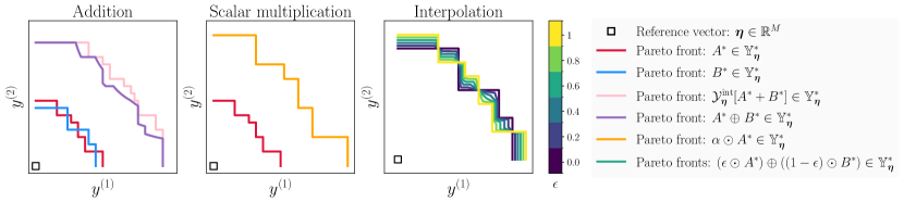
Figure 5: An illustration of some algebraic operations on the space of Pareto front surfaces in $M=2$ dimensions. For these examples, we set the scalar multipliers to be $\alpha=2$ and $\epsilon\in\{0.0,0.2,0.4,0.6,0.8,1.0\}$.

3.2 Utility functions

Utility functions are often used in multi-objective optimisation in order to assess the quality of a Pareto front approximation. In this section, we introduce a family of utility functions based on the length scalarisation function (2). We show that this family of utility functions are both interpretable and satisfy many desirable properties such as strict Pareto compliancy (Proposition 3.2).

Length-based R2 utility

The R2 utilities (Hansen and Jaszkiewicz, 1998) are a special family of utility functions that are constructed using scalarisation functions. They possess many general and desirable properties (Tu et al., 2024) which makes them very appealing to work with. By using the length scalarisation function (2), we define a special subfamily of the R2 utilities which we call the length-based R2 utilities. Precisely, a utility function is a length-based R2 utility if it can be written in the form

$$U_{\boldsymbol{\eta},\tau}[Y]:=\mathbb{E}_{\boldsymbol{\lambda}\sim\text{Uniform}(\mathcal{S}_{+}^{M-1})}\biggl{[}\max_{\mathbf{y}\in Y}\tau(s_{\boldsymbol{\eta},\boldsymbol{\lambda}}(\mathbf{y}))\biggr{]}=\mathbb{E}_{\boldsymbol{\lambda}\sim\text{Uniform}(\mathcal{S}_{+}^{M-1})}\bigl{[}\tau(\ell_{\boldsymbol{\eta},\boldsymbol{\lambda}}[\mathcal{Y}_{\boldsymbol{\eta}}^{\text{int}}[Y]])\bigr{]},$$ (6)

for any finite set of objective vectors $Y\subset\mathbb{R}^{M}$, where $\tau:\mathbb{R}_{\geq 0}\rightarrow\mathbb{R}$ is any strictly monotonically increasing transformation that is defined over the space of non-negative scalars. In words, this family of utility functions assesses the quality of a Pareto front approximation based on some notion of the average length away from the reference vector $\boldsymbol{\eta}\in\mathbb{R}^{M}$. In this setting, a greater utility is more desirable because it means that the set is much further away, on average, from the reference vector.

Hypervolume indicator

A special case of these length-based R2 utilities is the hypervolume indicator (Zitzler and Thiele, 1998), which is a popular performance metric in multi-objective optimisation. The hypervolume indicator of a finite set $Y\subset\mathbb{R}^{M}$ is defined as the volume of its truncated domination region:

$$U_{\boldsymbol{\eta}}^{\text{HV}}[Y]:=\nu[\mathbb{D}_{\preceq,\boldsymbol{\eta}}[Y]]=\mathbb{E}_{\boldsymbol{\lambda}\sim\text{Uniform}(\mathcal{S}_{+}^{M-1})}\biggl{[}\max_{\mathbf{y}\in Y}c_{M}(s_{\boldsymbol{\eta},\boldsymbol{\lambda}}(\mathbf{y}))^{M}\biggr{]}$$ (7)

where $\nu[A]:=\int_{\mathbb{R}^{M}}\mathbbm{1}[\mathbf{y}\in A]d\mathbf{y}$ is the Lebesgue measure on $\mathbb{R}^{M}$ with $A\subset\mathbb{R}^{M}$ denoting a measurable set and $\mathbbm{1}$ denoting the indicator function. The second equality above in (7) shows that the hypervolume indicator can be written in terms of a transformation of the length scalarisation function $\tau^{\text{HV}}(x)=c_{M}x^{M}$, where $c_{M}=\pi^{M/2}2^{-M}\Gamma(M/2+1)^{-1}$ is a positive scalar depending on the Gamma function $\Gamma(z)=\int_{0}^{\infty}t^{z-1}e^{-t}dt$. This equality has been proved in many earlier works (Shang et al., 2018; Deng and Zhang, 2019; Zhang and Golovin, 2020). In the left of Figure 6, we present a simple illustration of the hypervolume indicator in two dimensions.

Remark 3.5 (Hypervolume scalarisation)

The hypervolume scalarised value can also be interpreted geometrically as being equal to the volume of the hypersphere with diameter $s_{\boldsymbol{\eta},\boldsymbol{\lambda}}(\mathbf{y})\geq 0$, that is $\tau^{\textnormal{HV}}(s_{\boldsymbol{\eta},\boldsymbol{\lambda}}(\mathbf{y}))=\nu[\{\mathbf{z}\in\mathbb{R}^{M}:||\mathbf{z}||_{L^{2}}\leq s_{\boldsymbol{\eta},\boldsymbol{\lambda}}(\mathbf{y})/2\}]$ for any objective vector $\mathbf{y}\in\mathbb{R}^{M}$—see the right of Figure 4 for a visualisation of this interpretation in two dimensions.

General properties

By design, the length-based R2 utilities (6) inherit all of the standard properties that any R2 utility satisfies such as the monotone and submodularity property (Tu et al., 2024). In the following, we will additionally show that this special subfamily of utility functions also satisfies the strict Pareto compliancy property over the truncated space (Proposition 3.2). Loosely speaking, the strict Pareto compliancy property (Definition 3.3) states that if a set of vectors is strictly better than another, then it should have a higher utility. This result follows immediately from the fact that the hypervolume indicator is strictly Pareto compliant over the truncated space (Zitzler et al., 2003). We prove this result in Section A.4.

Definition 3.2 (Set domination)

Consider the subsets $A,B\subset\mathbb{R}^{M}$, we say that the set $A$ weakly or strictly dominates the set $B$ if and only if its weak Pareto domination region weakly or strictly contains the other, respectively:

$$A\succeq B \iff\mathbb{D}_{\preceq}[A]\supseteq\mathbb{D}_{\preceq}[B],$$

$$A\succ B \iff\mathbb{D}_{\preceq}[A]\supset\mathbb{D}_{\preceq}[B].$$

Definition 3.3 (Strict Pareto compliancy)

A utility function $U:2^{\mathbb{R}^{M}}\rightarrow\mathbb{R}$ is strictly Pareto compliant over a set $Y\subseteq\mathbb{R}^{M}$, if for all finite sets $A,B\subseteq Y$, we have that $A\succ B\implies U(A)>U(B)$.

Proposition 3.2 (Strict Pareto compliancy)

For any reference vector $\boldsymbol{\eta}\in\mathbb{R}^{M}$ and strictly monotonically increasing transformation $\tau:\mathbb{R}_{\geq 0}\rightarrow\mathbb{R}$, the corresponding length-based R2 utility (6) satisfies the strict Pareto compliancy property over the truncated space $\mathbb{D}_{\succ\mathrel{\mkern-5.0mu}\succ}[\{\boldsymbol{\eta}\}]\subset\mathbb{R}^{M}$.

3.3 Loss functions

Loss functions are an important aspect of decision theory because they quantify the cost associated with observing one element when we expected another. In this section, we define the frontier loss functions, which is a family of loss functions acting on the space of Pareto front surfaces, or more generally the space of polar surfaces $\mathbb{L}_{\boldsymbol{\eta}}$. These loss functions are useful because they give us a way to compare between any two Pareto front surfaces. Later on in Section 4.7, we will show how these loss functions can be used in order to define various probabilistic concepts on the space of random Pareto front surfaces.

Frontier loss

We define the frontier loss function $\mathcal{D}_{\boldsymbol{\eta},S}:\mathbb{L}_{\boldsymbol{\eta}}\times\mathbb{L}_{\boldsymbol{\eta}}\rightarrow\mathbb{R}_{\geq 0}$ as the average loss incurred along each reference line, that is

$$\mathcal{D}_{\boldsymbol{\eta},S}[A,B]:=\mathbb{E}_{\boldsymbol{\lambda}\sim\text{Uniform}(\mathcal{S}_{+}^{M-1})}[S(\ell_{\boldsymbol{\eta},\boldsymbol{\lambda}}[A],\ell_{\boldsymbol{\eta},\boldsymbol{\lambda}}[B])]$$ (8)

for any two polar surfaces $A,B\in\mathbb{L}_{\boldsymbol{\eta}}$, where $S:\mathbb{R}\times\mathbb{R}\rightarrow\mathbb{R}_{\geq 0}$ denotes a non-negative scoring function (or loss function). Clearly, different choices of scoring functions will lead to different notions of loss. For example, in Table 1, we present some popular scoring functions which are commonly used in the field of probabilistic forecasting—see Gneiting (2011) for discussion.

Frontier distance

If the scoring function $S$ is a metric in $\mathbb{R}$, then the resulting frontier loss function can be interpreted as a type of distance function over the space of polar surfaces $\mathbb{L}_{\boldsymbol{\eta}}$. Note though that this frontier distance function will only be a pseudometric in $\mathbb{L}_{\boldsymbol{\eta}}$. That is, unlike a metric, the distance between any two polar surfaces $A,B\in\mathbb{L}_{\boldsymbol{\eta}}$ will be zero, $\mathcal{D}_{\boldsymbol{\eta},S}[A,B]=0$, if and only if $\nu[\{\ell_{\boldsymbol{\eta},\boldsymbol{\lambda}}[A]\neq\ell_{\boldsymbol{\eta},\boldsymbol{\lambda}}[B]:\boldsymbol{\lambda}\in\mathcal{S}_{+}^{M-1}\}]=0$. In other words, the polar surfaces $A,B\in\mathbb{L}_{\boldsymbol{\eta}}$ are equivalent under this frontier distance if and only if their projected lengths disagree on a set of measure zero.

Hypervolume distance

A special and interpretable case of the frontier distance function is the hypervolume distance. The hypervolume distance between any two Pareto front surfaces is the volume of the symmetric difference between their corresponding truncated dominated regions. Specifically, if we restrict the distance function to the space of Pareto front surfaces $\mathbb{Y}^{*}_{\boldsymbol{\eta}}$ and set $S^{\text{HV}}(x,y):=|\tau^{\text{HV}}(x)-\tau^{\text{HV}}(y)|$, then we recover the hypervolume distance

$$\begin{split}\mathcal{D}_{\boldsymbol{\eta},S^{\text{HV}}}[A^{*},B^{*}]&:=\nu[\mathbb{D}_{\preceq,\boldsymbol{\eta}}[A^{*}]\triangle\mathbb{D}_{\preceq,\boldsymbol{\eta}}[B^{*}]]=2U_{\boldsymbol{\eta}}^{\text{HV}}[A^{*}\cup B^{*}]-U_{\boldsymbol{\eta}}^{\text{HV}}[A^{*}]-U_{\boldsymbol{\eta}}^{\text{HV}}[B^{*}]\end{split}$$ (9)

for any Pareto front surfaces $A^{*},B^{*}\in\mathbb{Y}^{*}_{\boldsymbol{\eta}}$, where $A\triangle B=(A\setminus B)\cup(B\setminus A)$ denotes the symmetric difference between the sets $A,B\subset\mathbb{R}^{M}$—see the right of Figure 6 for an illustration of this distance function on a two-dimensional example.

Remark 3.6 (Generalised frontier loss)

The frontier loss in (8) is defined using the length scalarisation function (2) and a uniform distribution over the scalarisation parameters. Naturally, we can generalise this construction further by considering an arbitrary scalarisation function and parameter distribution. This generalisation bares some similarity with the construction of the R2 utilities (Hansen and Jaszkiewicz, 1998; Tu et al., 2024).

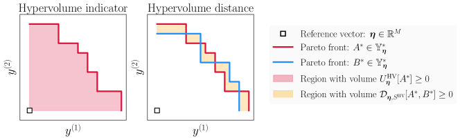
Figure 6: An illustration of the hypervolume indicator and hypervolume distance in $M=2$ dimensions.

4 Pareto front surface statistics

Real-world problems are typically noisy and subject to many sources of uncertainty. In order to quantify this uncertainty, decision makers often appeal to ideas from probability and statistics. In this section, we will generalise these existing ideas to function over the space of Pareto front surfaces $\mathbb{Y}^{*}_{\boldsymbol{\eta}}$. Precisely, we will study the concept of a random Pareto front surface and showcase how our polar parametrisation result (Theorem 3.1) can be easily used in order to define many statistical quantities of interest. Intuitively, we will treat the Pareto front surface as an infinite-dimensional stochastic process (10) and define the statistics according to its corresponding finite-dimensional distributions. Before we introduce these ideas in more detail, we will first describe the general set up and assumptions that we will be using throughout this section.

Formulation

Consider a probability space $(\Omega,\mathcal{F},\mathbb{P})$, where $\Omega$ denotes the sample space, $\mathcal{F}$ denotes a $\sigma$-algebra and $\mathbb{P}$ denotes a probability measure. In this section, we will be interested in studying the Pareto front surface associated with some vector-valued stochastic process $f:\mathbb{X}\times\Omega\rightarrow\mathbb{R}^{M}$, which we have indexed with the inputs $\mathbf{x}\in\mathbb{X}$. For a fixed and known reference vector $\boldsymbol{\eta}\in\mathbb{R}^{M}$, we denote the corresponding Pareto front surface by

$$\begin{split}Y_{\boldsymbol{\eta},f}^{*}(\boldsymbol{\omega})&:=\mathcal{Y}_{\boldsymbol{\eta}}^{\textnormal{int}}[\{f(\mathbf{x},\boldsymbol{\omega})\}_{\mathbf{x}\in\mathbb{X}}]=\biggl{\{}\boldsymbol{\eta}+\sup_{\mathbf{x}\in\mathbb{X}}s_{\boldsymbol{\eta},\boldsymbol{\lambda}}(f(\mathbf{x},\boldsymbol{\omega}))\boldsymbol{\lambda}\in\mathbb{R}^{M}:\boldsymbol{\lambda}\in\mathcal{S}_{+}^{M-1}\biggr{\}},\end{split}$$ (10)

for $\boldsymbol{\omega}\in\Omega$, where $\ell_{\boldsymbol{\eta},\boldsymbol{\lambda}}[Y_{\boldsymbol{\eta},f}^{*}(\boldsymbol{\omega})]=\sup_{\mathbf{x}\in\mathbb{X}}s_{\boldsymbol{\eta},\boldsymbol{\lambda}}(f(\mathbf{x},\boldsymbol{\omega}))\geq 0$ are the corresponding the projected lengths along the positive directions $\boldsymbol{\lambda}\in\mathcal{S}_{+}^{M-1}$.

Projected length process

By exploiting the explicit form of the random Pareto front surface in (10), we see that the only dependence on the random quantity $\boldsymbol{\omega}\in\Omega$ arises solely in the projected lengths $\ell_{\boldsymbol{\eta},\boldsymbol{\lambda}}[Y_{\boldsymbol{\eta},f}^{*}(\boldsymbol{\omega})]\geq 0$ for $\boldsymbol{\lambda}\in\mathcal{S}_{+}^{M-1}$. Therefore all of the distributional information about the Pareto front surface is completely characterised by its projected length process

$$\mathcal{L}_{\boldsymbol{\eta}}(\boldsymbol{\omega}):=\{\ell_{\boldsymbol{\eta},\boldsymbol{\lambda}}[Y_{\boldsymbol{\eta},f}^{*}(\boldsymbol{\omega})]\geq 0:\boldsymbol{\lambda}\in\mathcal{S}_{+}^{M-1}\}.$$ (11)

Note that if we used a nonlinear representation for the Pareto front surface instead (Remark 3.3), then it is unlikely that such a simplification would have been possible.

Assumptions

To avoid dealing with some unnecessary complications, we will make the following two simplifying assumptions. Firstly, we have Assumption 4.1, which states that the Pareto front surface of interest is non-empty almost surely. Secondly, we have Assumption 4.2, which states that the stochastic process of interest is bounded almost surely. Together, both of these results ensures that the polar parametrisation of the Pareto front surface, described on the right of (10), holds almost surely. Moreover, Assumption 4.2 also ensures that the projected length $\ell_{\boldsymbol{\eta},\boldsymbol{\lambda}}[Y_{\boldsymbol{\eta},f}^{*}]\geq 0$, along any positive direction $\boldsymbol{\lambda}\in\mathcal{S}_{+}^{M-1}$, is bounded almost surely. Consequently, this means that the moments and quantiles of the projected lengths exist and are finite.

Assumption 4.1 (Positive lengths)

The Pareto front surface $Y_{\boldsymbol{\eta},f}^{*}$ is non-empty almost surely.

Assumption 4.2 (Bounded lengths)

The stochastic process $f$ is bounded almost surely.

Remark 4.1 (Finite input space)

All of the results in this section hold for any input space $\mathbb{X}$. Nevertheless, for computational convenience, most of the examples in this section focus on the practical setting where the input space is finite $|\mathbb{X}|<\infty$. This implies that the projected lengths can be computed exactly because the supremum reduces down to a maximum: $\ell_{\boldsymbol{\eta},\boldsymbol{\lambda}}[Y_{\boldsymbol{\eta},f}^{*}(\boldsymbol{\omega})]=\max_{\mathbf{x}\in\mathbb{X}}s_{\boldsymbol{\eta},\boldsymbol{\lambda}}(f(\mathbf{x},\boldsymbol{\omega}))$ for $\boldsymbol{\lambda}\in\mathcal{S}_{+}^{M-1}$.

Remark 4.2 (Sensitivity to transformations)

Most of the probabilistic concepts which we describe in this section are sensitive to the choice of reference vector (Remark 2.1) and any nonlinear transformations of the objective space (Remark 3.3). For example, in Section 4.1, we define the expected Pareto front surface in the original objective space: $\mathbb{E}_{\boldsymbol{\omega}}[Y_{\boldsymbol{\eta},f}^{*}(\boldsymbol{\omega})]\in\mathbb{Y}^{*}_{\boldsymbol{\eta}}$. But we could have quite easily defined the same expectation in the transformed space, before inverting it back to the original objective space: $\tau^{-1}(\mathbb{E}_{\boldsymbol{\omega}}[Y_{\tau(\boldsymbol{\eta}),\tau\circ f}^{*}(\boldsymbol{\omega})])$, where $\tau:\mathbb{R}^{M}\rightarrow\mathbb{R}^{M}$ is an invertible monotonically increasing function. Clearly, these two quantities are not necessarily equal and therefore some care has to be taken when using one or the other. Note that this issue also arises for the scalar-valued setting as well: $\mathbb{E}[\max_{n}A_{n}]\neq\tau^{-1}(\mathbb{E}[\max_{n}\tau(A_{n})])$ for any collection of scalar-valued random variable $A_{n}$ and any invertible monotonically increasing transformation $\tau:\mathbb{R}\rightarrow\mathbb{R}$.

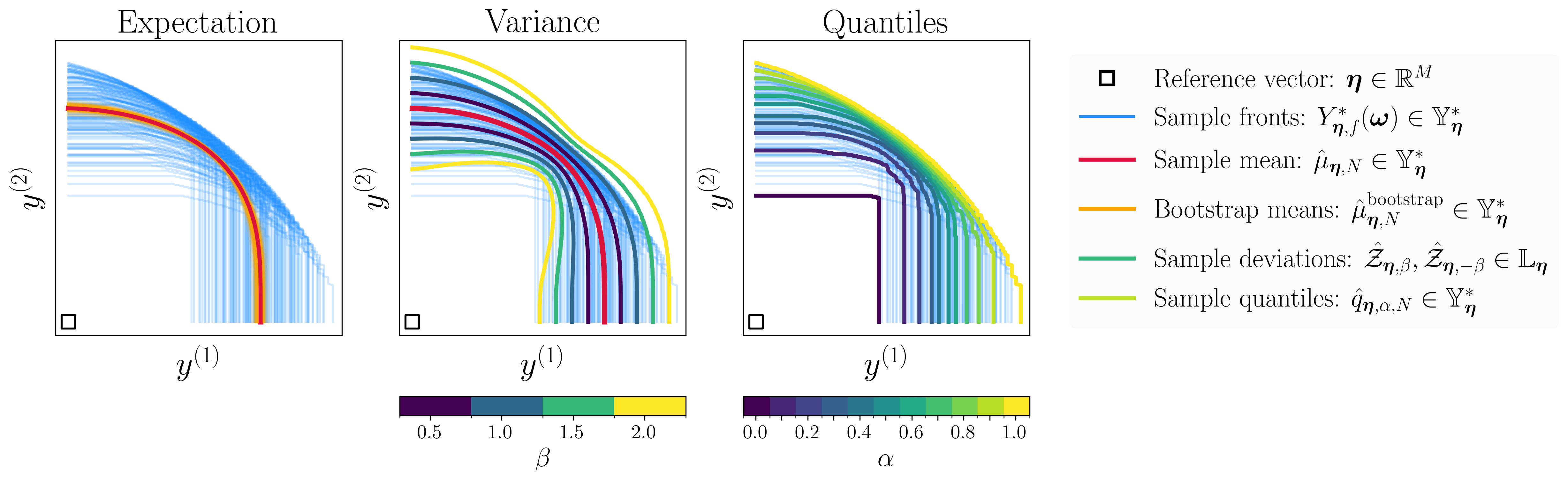
Figure 7: An illustration of the estimated Pareto front surface statistics for a finite set of samples in $M=2$ dimensions.

4.1 Expectation

We define the expected value of the Pareto front surface distribution (10) by the equation

$$\mathbb{E}_{\boldsymbol{\omega}}[Y_{\boldsymbol{\eta},f}^{*}(\boldsymbol{\omega})]:=\{\boldsymbol{\eta}+\mathbb{E}_{\boldsymbol{\omega}}[\ell_{\boldsymbol{\eta},\boldsymbol{\lambda}}[Y_{\boldsymbol{\eta},f}^{*}(\boldsymbol{\omega})]]\boldsymbol{\lambda}\in\mathbb{R}^{M}:\boldsymbol{\lambda}\in\mathcal{S}_{+}^{M-1}\},$$ (12)

where $\mathbb{E}_{\boldsymbol{\omega}}[\cdot]$ denotes the expectation operator under $\mathbb{P}$. It can be easily shown that under the given assumptions, the expectation above satisfies the conditions in Proposition 3.1 and therefore is a valid Pareto front surface. For completeness, we state this result in Proposition 4.1 and prove it in Section A.5.

Proposition 4.1

Under Assumptions 4.1 and 4.2, the expectation of a Pareto front surface distribution (12) is a Pareto front surface $\mathbb{E}_{\boldsymbol{\omega}}[Y_{\boldsymbol{\eta},f}^{*}(\boldsymbol{\omega})]\in\mathbb{Y}^{*}_{\boldsymbol{\eta}}$.

Sample-based estimate

In general, the expected projected lengths is an intractable quantity that cannot be computed exactly. Nevertheless, if we can sample a collection of random Pareto front surfaces, then we can easily estimate this quantity using a sample average

$$\hat{\mu}_{\boldsymbol{\eta},\boldsymbol{\lambda},N}=\frac{1}{N}\sum_{n=1}^{N}\ell_{\boldsymbol{\eta},\boldsymbol{\lambda}}[Y_{\boldsymbol{\eta},f}^{*}(\boldsymbol{\omega}_{n})]$$ (13)

for $\boldsymbol{\lambda}\in\mathcal{S}_{+}^{M-1}$, where $\boldsymbol{\omega}_{n}\in\Omega$ denotes some independent samples of the random parameter. Consequently, we can then define the sample mean Pareto front surface $\hat{\mu}_{\boldsymbol{\eta},N}\in\mathbb{Y}^{*}_{\boldsymbol{\eta}}$ using the projected length estimates given by (13). The fact that this estimated front is also a valid Pareto front surface is a direct consequence of Proposition 4.1. We illustrate an example of the estimated mean Pareto front surface in the left plot of Figure 7.

Remark 4.3 (Bayesian bootstrap)

To quantify some uncertainty about the mean estimate, we can appeal to the use many traditional techniques from scalar-valued statistics. For example, we can construct a Bayesian bootstrap (Rubin, 1981) of the estimated means

$$\hat{\mu}^{\textnormal{bootstrap}}_{\boldsymbol{\eta},\boldsymbol{\lambda},N}(\mathbf{w})=\sum_{n=1}^{N}w^{(n)}\ell_{\boldsymbol{\eta},\boldsymbol{\lambda}}[Y_{\boldsymbol{\eta},f}^{*}(\boldsymbol{\omega}_{n})],$$

where $\mathbf{w}=(w^{(1)},\dots,w^{(N)})\sim\text{Uniform}(\Delta^{M-1})$ denotes a weight vector sampled from a uniform distribution over the probability simplex $\Delta^{M-1}:=\{\mathbf{w}\in\mathbb{R}^{M}_{\geq 0}:||\mathbf{w}||_{L^{1}}=1\}$. We demonstrate an example of these bootstrap estimates in the left plot of Figure 7. Note that a similar type of bootstrap estimate can also be computed for the other Pareto front surface statistics which we will introduce in the upcoming sections.

4.2 Covariance

We define the covariance of the Pareto front surface distribution (10) as the corresponding collection of covariance matrices with

$$\begin{split}\text{Cov}_{\boldsymbol{\omega}}[Y_{\boldsymbol{\eta},f}^{*}(\boldsymbol{\omega}),Y_{\boldsymbol{\eta},f}^{*}(\boldsymbol{\omega})]_{\boldsymbol{\lambda}_{i},\boldsymbol{\lambda}_{j}}&:=\boldsymbol{\lambda}_{i}\boldsymbol{\lambda}_{j}^{T}\text{Cov}_{\boldsymbol{\omega}}[\ell_{\boldsymbol{\eta},\boldsymbol{\lambda}_{i}}[Y_{\boldsymbol{\eta},f}^{*}(\boldsymbol{\omega})],\ell_{\boldsymbol{\eta},\boldsymbol{\lambda}_{j}}[Y_{\boldsymbol{\eta},f}^{*}(\boldsymbol{\omega})]]\in\mathbb{R}^{M\times M}\end{split}$$ (14)

for any two positive unit vectors $\boldsymbol{\lambda}_{i},\boldsymbol{\lambda}_{j}\in\mathcal{S}_{+}^{M-1}$, where $\text{Cov}_{\boldsymbol{\omega}}[\cdot,\cdot]$ denotes the covariance operator under $\mathbb{P}$.

Sample-based estimate

In general, the covariance of the projected lengths is an intractable quantity that cannot be computed exactly. Nevertheless, if we can sample a collection of random Pareto front surfaces, then we can easily estimate these terms by using the standard sample-based estimate

$$\hat{\sigma}^{2}_{\boldsymbol{\eta},\boldsymbol{\lambda}_{i},\boldsymbol{\lambda}_{i},N}=\frac{1}{N-1}\sum_{n=1}^{N}(\ell_{\boldsymbol{\eta},\boldsymbol{\lambda}_{i}}[Y_{\boldsymbol{\eta},f}^{*}(\boldsymbol{\omega}_{n})]-\hat{\mu}_{\boldsymbol{\eta},\boldsymbol{\lambda}_{i},N})(\ell_{\boldsymbol{\eta},\boldsymbol{\lambda}_{j}}[Y_{\boldsymbol{\eta},f}^{*}(\boldsymbol{\omega}_{n})]-\hat{\mu}_{\boldsymbol{\eta},\boldsymbol{\lambda}_{j},N})$$

for any two positive unit vectors $\boldsymbol{\lambda}_{i},\boldsymbol{\lambda}_{j}\in\mathcal{S}_{+}^{M-1}$, where $\boldsymbol{\omega}_{n}\in\Omega$ denotes some independent samples of the random parameter with $N>1$.

Marginal deviation surfaces

The marginal variances can be used in order to define an uncertainty region around the mean. That is, we can define the upper deviation surface $\mathcal{Z}_{\boldsymbol{\eta},\beta}$ and lower deviation surface $\mathcal{Z}_{\boldsymbol{\eta},-\beta}$ for some $\beta\geq 0$ by

$$\mathcal{Z}_{\boldsymbol{\eta},\beta}:=\{\boldsymbol{\eta}+(\mu_{\boldsymbol{\eta},\boldsymbol{\lambda}}+\beta\sigma_{\boldsymbol{\eta},\boldsymbol{\lambda},\boldsymbol{\lambda}})_{+}\boldsymbol{\lambda}\in\mathbb{R}^{M}:\boldsymbol{\lambda}\in\mathcal{S}_{+}^{M-1}\}\in\mathbb{L}_{\boldsymbol{\eta}}$$

where $\sigma_{\boldsymbol{\eta},\boldsymbol{\lambda},\boldsymbol{\lambda}}:=(\sigma^{2}_{\boldsymbol{\eta},\boldsymbol{\lambda},\boldsymbol{\lambda}})^{1/2}$ denotes the marginal standard deviation in the direction $\boldsymbol{\lambda}\in\mathcal{S}^{M-1}_{+}$ and $(x)_{+}:=\max(x,0)$, for $x\in\mathbb{R}$, denotes the truncation function which is used to ensure that the lengths are non-negative. Note that these polar surfaces are not necessarily Pareto front surfaces because they do not necessarily satisfy the maximum ratio condition in Proposition 3.1. We present an illustration of these deviation surfaces in the middle plot of Figure 7 for a simple two-dimensional problem.

4.3 Quantiles

We define the quantiles of the Pareto front surface distribution (10) as the collection of marginal quantiles

$$\mathcal{Q}_{\boldsymbol{\omega}}[Y_{\boldsymbol{\eta},f}^{*}(\boldsymbol{\omega}),\alpha] :=\{\boldsymbol{\eta}+\mathcal{Q}_{\boldsymbol{\omega}}[\ell_{\boldsymbol{\eta},\boldsymbol{\lambda}}[Y_{\boldsymbol{\eta},f}^{*}(\boldsymbol{\omega})],\alpha]\boldsymbol{\lambda}\in\mathbb{R}^{M}:\boldsymbol{\lambda}\in\mathcal{S}_{+}^{M-1}\},$$ (15)

where $\mathcal{Q}_{\boldsymbol{\omega}}[\cdot,\alpha]$ denotes the the $\alpha$-level quantile operator under $\mathbb{P}$ for any $\alpha\in(0,1)$. It can be easily shown that under the given assumptions, the quantiles above satisfies the conditions in Proposition 3.1 and therefore is a valid Pareto front surface. For completeness, we state this result in Proposition 4.2 and prove it in Section A.6.

Proposition 4.2

Under Assumptions 4.1 and 4.2, for any $\alpha\in(0,1)$, the $\alpha$-quantile of a Pareto front surface distribution (15) is a Pareto front surface $\mathcal{Q}_{\boldsymbol{\omega}}[Y_{\boldsymbol{\eta},f}^{*}(\boldsymbol{\omega}),\alpha]\in\mathbb{Y}^{*}_{\boldsymbol{\eta}}$.

Interpretation

Note that the $\alpha$-level quantile (15) does not imply that 100$\alpha$% of the possible Pareto front surfaces are weakly dominated by this quantile Pareto front surface. Instead, this definition of the quantile can be interpreted as a surface which divides the truncated objective space $\mathbb{D}_{\succ\mathrel{\mkern-5.0mu}\succ}[\{\boldsymbol{\eta}\}]$ into two regions. One region is the space dominated by the $\alpha$-level quantile, which contains at least $\alpha$-probability. Whilst the other region, its complement, contains at most ($1-\alpha$)-probability. This interpretation follows immediately from the alternative formulation of the $\alpha$-quantiles described in (20), which are based on the concept of domination probabilities (Section 4.4).

Sample-based estimates

In general, the quantile of the projected lengths is an intractable quantity that cannot be computed exactly. Nevertheless, if we can sample a collection of random Pareto front surfaces, then we can easily estimate these quantiles by using an empirical estimate

$$\hat{q}_{\boldsymbol{\eta},\boldsymbol{\lambda},\alpha,N}:=\mathcal{Q}_{\boldsymbol{\omega}\sim\text{Uniform}(\{\mathbf{w}_{n}\}_{n\leq N})}[\ell_{\boldsymbol{\eta},\boldsymbol{\lambda}}[Y_{\boldsymbol{\eta},f}^{*}(\boldsymbol{\omega})],\alpha]$$ (16)

for $\boldsymbol{\lambda}\in\mathcal{S}_{+}^{M-1}$, where $\boldsymbol{\omega}_{n}\in\Omega$ denotes some independent samples of the random parameter. Consequently, we can then define the empirical quantile Pareto front surface $\hat{q}_{\boldsymbol{\eta},\alpha,N}\in\mathbb{Y}^{*}_{\boldsymbol{\eta}}$ using the projected lengths estimates given by (16). By Proposition 4.2, this empirical Pareto front surface is indeed a valid Pareto front surface. We illustrate an example of this empirical quantile front in the right plot of Figure 7.

4.4 Probability of domination

The probability that a vector or a set of vectors is Pareto optimal is given by the probability of domination. This probability can also be interpreted as a generalisation of the survival function for Pareto front surface distributions. By Lemma 3.1, we can write the probability of domination in term of the projected lengths

$$\begin{split}\mathbb{P}[Y\subseteq\mathbb{D}_{\preceq,\boldsymbol{\eta}}[Y^{*}_{\boldsymbol{\eta},f}]]&=\mathbb{P}[\land_{\mathbf{y}\in Y}(s_{\boldsymbol{\eta},\boldsymbol{\lambda}_{\boldsymbol{\eta}}^{*}(\mathbf{y})}(\mathbf{y})\leq\ell_{\boldsymbol{\eta},\boldsymbol{\lambda}_{\boldsymbol{\eta}}^{*}(\mathbf{y})}[Y^{*}_{\boldsymbol{\eta},f}])]\\ &=\mathbb{P}\biggl{[}\inf_{\mathbf{y}\in Y}\frac{\ell_{\boldsymbol{\eta},\boldsymbol{\lambda}_{\boldsymbol{\eta}}^{*}(\mathbf{y})}[Y^{*}_{\boldsymbol{\eta},f}]}{||\mathbf{y}-\boldsymbol{\eta}||_{L^{2}}}\geq 1\biggr{]},\end{split}$$ (17)

for any set of vectors $Y\subseteq\mathbb{D}_{\succ\mathrel{\mkern-5.0mu}\succ}[\{\boldsymbol{\eta}\}]$, where $\land$ denotes the logical and operation. In practice, this probability is an intractable quantity. Nevertheless, if we can sample a collection of random Pareto front surfaces, then we can easily estimate it by using a simple Monte Carlo average: $\mathbb{P}[I(\boldsymbol{\omega})]\approx\frac{1}{N}\sum_{n=1}^{N}\mathbbm{1}[I(\boldsymbol{\omega}_{n})]$, where $I(\boldsymbol{\omega})\in\{0,1\}$ denotes a random boolean variable and $\boldsymbol{\omega}_{n}\in\Omega$ denotes some independent samples of the random parameter. In the left plot of Figure 8, we visualise the contours associated with the estimated marginal domination probabilities for the Pareto front surface distribution described in Figure 7.

4.5 Probability of deviation

In some cases, we might be interested in computing the probability that a vector or a set of vectors lies between two potentially random Pareto front surfaces. We refer to this quantity as the probability of deviation. By using Lemma 3.1, we can write the probability of deviation in term of the projected lengths

$$\begin{split}&\mathbb{P}[Y\subseteq(\mathbb{D}_{\preceq,\boldsymbol{\eta}}[A^{*}]\triangle\mathbb{D}_{\preceq,\boldsymbol{\eta}}[B^{*}])\setminus\mathcal{Y}^{\textnormal{int}}_{\boldsymbol{\eta}}[A^{*}\cup B^{*}]]\\ &=\mathbb{P}\biggl{[}\land_{\mathbf{y}\in Y}\Bigl{(}\min_{Y^{*}\in\{A^{*},B^{*}\}}\ell_{\boldsymbol{\eta},\boldsymbol{\lambda}_{\boldsymbol{\eta}}^{*}(\mathbf{y})}[Y^{*}]<s_{\boldsymbol{\eta},\boldsymbol{\lambda}_{\boldsymbol{\eta}}^{*}(\mathbf{y})}(\mathbf{y})<\max_{Y^{*}\in\{A^{*},B^{*}\}}\ell_{\boldsymbol{\eta},\boldsymbol{\lambda}_{\boldsymbol{\eta}}^{*}(\mathbf{y})}[Y^{*}]\Bigr{)}\biggr{]}\\ &=\mathbb{P}\biggl{[}\sup_{\mathbf{y}\in Y}\biggl{(}\frac{\ell_{\boldsymbol{\eta},\boldsymbol{\lambda}_{\boldsymbol{\eta}}^{*}(\mathbf{y})}[A^{*}]}{||\mathbf{y}-\boldsymbol{\eta}||_{L^{2}}}-1\biggr{)}\biggl{(}\frac{\ell_{\boldsymbol{\eta},\boldsymbol{\lambda}_{\boldsymbol{\eta}}^{*}(\mathbf{y})}[B^{*}]}{||\mathbf{y}-\boldsymbol{\eta}||_{L^{2}}}-1\biggr{)}<0\biggr{]},\end{split}$$ (18)

for any random Pareto front surfaces $A^{*}(\boldsymbol{\omega}),B^{*}(\boldsymbol{\omega})\in\mathbb{Y}^{*}_{\boldsymbol{\eta}}$ and any set vectors $Y\subseteq\mathbb{D}_{\succ\mathrel{\mkern-5.0mu}\succ}[\{\boldsymbol{\eta}\}]$. As with the domination probabilities in (17), this quantity can be easily estimated using a Monte Carlo average. In Figure 8, we give an illustration of the estimated marginal deviation probabilities when $A^{*}(\boldsymbol{\omega})=Y^{*}_{\boldsymbol{\eta},f}(\boldsymbol{\omega})$ is a random Pareto front surface and $B^{*}(\boldsymbol{\omega})=\mathbb{E}_{\boldsymbol{\omega}}[Y^{*}_{\boldsymbol{\eta},f}(\boldsymbol{\omega})]$ is a candidate for the expectation which is deterministic.

4.6 Vorob’ev statistics

Random set theory (Molchanov, 2005) gives us a way to extend standard concepts from probability and statistics to work over the space of closed sets. Some key ideas from this field have been used in earlier work in order to define some Pareto front surface statistics (Grunert da Fonseca and Fonseca, 2010; Binois et al., 2015a). Precisely, these ideas have focussed on defining probabilistic concepts over the space of domination regions $\mathcal{D}_{\preceq}:=\{\mathbb{D}_{\preceq}[A]\subset\mathbb{R}^{M}:A\subset\mathbb{R}^{M}\}$. In the following, we will review the core ideas within these works and show how they relate to our framework. To increase the generality of our discussion, we will consider working in the more general space of truncated domination regions $\mathcal{D}_{\preceq,\boldsymbol{\eta}}:=\{\mathbb{D}_{\preceq,\boldsymbol{\eta}}[A]\subset\mathbb{R}^{M}:A\subset\mathbb{R}^{M}\}$.

Coverage function

In random set theory, one often relies on the concept of a coverage function, which gives us the probability that an element lies within a random closed set. When working over the space of truncated domination regions $\mathcal{D}_{\preceq,\boldsymbol{\eta}}$, this coverage function is simply given by the probability of domination (17): $\mathbb{P}[\mathbf{y}\in\mathbb{D}_{\preceq,\boldsymbol{\eta}}[Y^{*}_{\boldsymbol{\eta},f}]]$ for any vector $\mathbf{y}\in\mathbb{R}^{M}$. Equipped with this coverage function, we can now define many different types of probabilistic concepts by leveraging ideas from random set theory. Notably, the existing works referenced above have primarily focussed on extending the Vorob’ev concepts of random set theory (Molchanov, 2005, Section 2.2), which we describe below.

Vorob’ev quantiles

The Vorob’ev $\alpha$-quantile is a possible generalisation of the quantile function which is defined using the coverage function. Mathematically, the Vorob’ev $\alpha$-quantile is defined as the $\alpha$-level excursion set associated with the coverage function

$$\begin{split}\mathcal{Q}^{\text{Vorob'ev}}_{\boldsymbol{\omega}}[Y^{*}_{\boldsymbol{\eta},f}(\boldsymbol{\omega}),\alpha]&:=\{\mathbf{y}\in\mathbb{R}^{M}:\mathbb{P}[\mathbf{y}\in\mathbb{D}_{\preceq,\boldsymbol{\eta}}[Y^{*}_{\boldsymbol{\eta},f}]]\geq\alpha\}\end{split}$$ (19)

for $\alpha\in(0,1)$. By Lemma 3.1, we see that the Vorob’ev $\alpha$-quantile (19) is equivalent to the truncated domination region of the $(1-\alpha)$-quantile front in (15), that is

$$\mathcal{Q}^{\text{Vorob'ev}}_{\boldsymbol{\omega}}[Y^{*}_{\boldsymbol{\eta},f}(\boldsymbol{\omega}),\alpha]=\mathbb{D}_{\preceq,\boldsymbol{\eta}}[\mathcal{Q}_{\boldsymbol{\omega}}[Y^{*}_{\boldsymbol{\eta},f}(\boldsymbol{\omega}),1-\alpha]].$$ (20)

In other words, the $\alpha$-level quantile in (15) is equal to the Pareto front surface or the upper isoline of the $(1-\alpha)$-level Vorob’ev quantile. Note that in the original work by Grunert da Fonseca and Fonseca (2010), they worked in the space of domination regions $\mathcal{D}_{\preceq}$ and therefore their result does not depend on the reference vector. Crudely speaking, we can recover this special case by letting the reference vector tend to negative infinity: $\boldsymbol{\eta}=(\epsilon,\dots,\epsilon)\in\mathbb{R}^{M}$ with $\epsilon\rightarrow-\infty$.

Vorob’ev mean

In addition to proposing the Vorob’ev $\alpha$-quantile, Grunert da Fonseca and Fonseca (2010) proposed using the median quantile ($\alpha=0.5$) as a potential candidate for the mean Pareto front surface. In contrast Binois et al. (2015a) proposed using the Vorob’ev expectation as a candidate for the mean. The Vorob’ev expectation is defined as the $\alpha^{*}$-level Vorob’ev quantile whose hypervolume is the closest to the expected hypervolume of the random Pareto front surface. Precisely, $\mathbb{E}^{\text{Vorob'ev}}_{\boldsymbol{\omega}}[Y^{*}_{\boldsymbol{\eta},f}(\boldsymbol{\omega})]:=\mathcal{Q}_{\boldsymbol{\omega}}^{\text{Vorob'ev}}[Y^{*}_{\boldsymbol{\eta},f}(\boldsymbol{\omega}),\alpha^{*}]$, where $\alpha^{*}$ satisfies the inequality

$$\nu[\mathcal{Q}^{\text{Vorob'ev}}_{\boldsymbol{\omega}}[Y^{*}_{\boldsymbol{\eta},f}(\boldsymbol{\omega}),\alpha]]\leq V_{\boldsymbol{\eta},f}\leq\nu[\mathcal{Q}^{\text{Vorob'ev}}_{\boldsymbol{\omega}}[Y^{*}_{\boldsymbol{\eta},f}(\boldsymbol{\omega}),\alpha^{*}]]$$ (21)

for any $\alpha>\alpha^{*}$, where $V_{\boldsymbol{\eta},f}:=\mathbb{E}_{\boldsymbol{\omega}}[\nu[\mathbb{D}_{\preceq,\boldsymbol{\eta}}[Y^{*}_{\boldsymbol{\eta},f}(\boldsymbol{\omega})]]]=\mathbb{E}_{\boldsymbol{\omega}}[U^{\text{HV}}_{\boldsymbol{\eta}}[Y^{*}_{\boldsymbol{\eta},f}(\boldsymbol{\omega})]]$ is the expected hypervolume of the Pareto front surface distribution. Note that the Vorob’ev mean is a Vorob’ev quantile and therefore it is a truncated domination region and not a Pareto front surface. As a result, when we later refer to the Vorob’ev mean front, we are actually referring to the Pareto front surface of the Vorob’ev mean, that is the $(1-\alpha^{*})$-quantile front.

Vorob’ev deviation

Analogous to how the traditional scalar-valued expectation minimises the variance, the Vorob’ev mean is known to minimise a quantity known as the Vorob’ev deviation. In the work by Binois et al. (2015a), they defined the Vorob’ev deviation of a Pareto front surface distribution as the expected hypervolume of the symmetric difference between the Pareto front surface and the considered set. Equivalently, the quantity can be written as the expected hypervolume distance (9) between these two sets, that is

$$\textsc{Vorob'evDeviation}_{\boldsymbol{\eta},f}[A] :=\mathbb{E}_{\boldsymbol{\omega}}[\nu[A\triangle\mathbb{D}_{\preceq,\boldsymbol{\eta}}[Y^{*}_{\boldsymbol{\eta},f}(\boldsymbol{\omega})]]]$$ (22)

for any measurable set $A\in\mathcal{M}(\mathbb{D}_{\succ\mathrel{\mkern-5.0mu}\succ}[\{\boldsymbol{\eta}\}])$ lying in the truncated space. As shown in the work by Molchanov (2005, Section 2.2), the Vorob’ev mean is a minimiser to the Vorob’ev deviation over the space of measurable sets $A\in\mathcal{M}(\mathbb{D}_{\succ\mathrel{\mkern-5.0mu}\succ}[\{\boldsymbol{\eta}\}])$ subject to the condition that $\nu[A]=V_{\boldsymbol{\eta},f}$. That is,

$$\mathbb{E}^{\text{Vorob'ev}}_{\boldsymbol{\omega}}[Y^{*}_{\boldsymbol{\eta},f}(\boldsymbol{\omega})]\in\operatorname*{arg\,min}_{A\in\mathcal{M}(\mathbb{D}_{\succ\mathrel{\mkern-5.0mu}\succ}[\{\boldsymbol{\eta}\}]):\nu[A]=V_{\boldsymbol{\eta},f}}\textsc{Vorob'evDeviation}_{\boldsymbol{\eta},f}[A].$$

Validity of the Pareto front surfaces

As a direct consequence of Proposition 4.2, the positive isolines of the Vorob’ev based Pareto front surfaces are all valid Pareto front surfaces because they are just instances of the quantile front (15). This result was taking for granted in the original works, but we have shown that it follows quite naturally from our polar parametrisation result.

Sample-based estimates

The Vorob’ev statistics above can be estimated using the empirical quantiles as we described in Section 4.3. For the Vorob’ev mean front, we have to additionally compute the parameter $\alpha^{*}$ which satisfies the hypervolume condition (21). To approximately solve this problem, Binois et al. (2015a) proposed using an iterative bisection scheme. Notably, this procedure can be very expensive because it requires evaluating the hypervolume of the quantiles several times. On the other hand, our definition of the expectation is much cheaper and simpler to estimate. In Figure 8, we present a visual comparison between the estimated Vorob’ev mean front and our sample mean front for a simple two-dimensional example. In this example, there does not appear to be any meaningful difference between these two Pareto front surfaces.

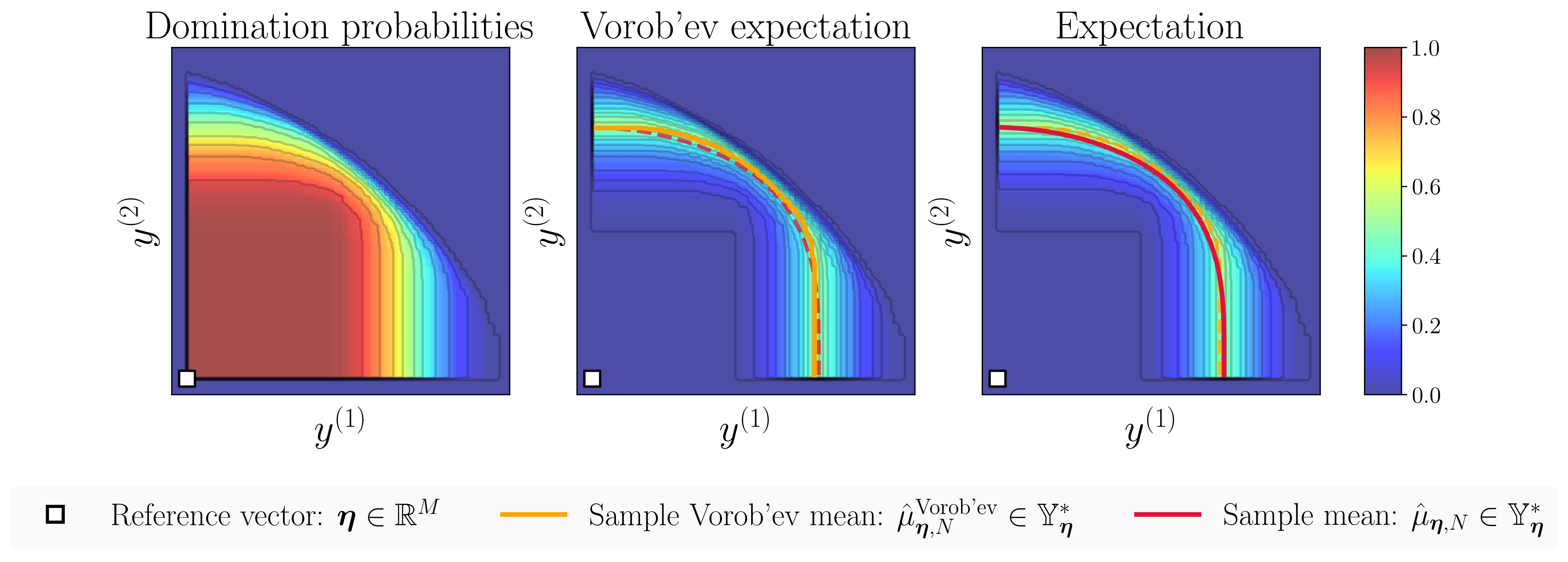
Figure 8: An illustration of the Vorob’ev statistics on an $M=2$ dimensional example. On the left plot, we illustrate the contours of the estimated marginal probability of domination (17). In the middle and right plot, we illustrate the estimated Vorob’ev mean front and expected front, respectively. For both of these fronts, we include the contours of the estimated marginal probability of deviation (18) between the random Pareto front surface and the mean estimate.

4.7 Decision-theoretic construction

Many standard concepts in probability, concerning real-valued random variables, can be constructed under the decision-theoretic perspective in which we optimise a certain scoring rule (Gneiting, 2011). Remarkably, our work on the polar parametrisation of the Pareto front surface gives us an easy way to generalise this decision-theoretic construction to the space of Pareto front surface distributions. In particular, we can recover many of the Pareto front surface statistics introduced in the previous sections as being equal to a functional $F_{\boldsymbol{\omega}}$, which minimises some expected frontier loss (8),

$$F_{\boldsymbol{\omega}}[Y_{\boldsymbol{\eta},f}^{*}(\boldsymbol{\omega})]\in\operatorname*{arg\,min}_{A\in\mathbb{L}_{\boldsymbol{\eta}}}\mathbb{E}_{\boldsymbol{\omega}}[\mathcal{D}_{\boldsymbol{\eta},S}[A,Y_{\boldsymbol{\eta},f}^{*}(\boldsymbol{\omega})]],$$ (23)

where $S:\mathbb{R}\times\mathbb{R}\rightarrow\mathbb{R}_{\geq 0}$ denotes some scoring function. In Table 1, we present the explicit choices of $S$ which leads to the different Pareto front surface statistics that we introduced earlier. Note that all of the results in this table follow immediately from the standard construction of these functionals in the univariate setting. To see this, we first note that we can rewrite the expected frontier loss as an expectation over the space of positive unit vectors by interchanging the order of integration, that is

$$\mathbb{E}_{\boldsymbol{\omega}}[\mathcal{D}_{\boldsymbol{\eta},S}[A,Y_{\boldsymbol{\eta},f}^{*}(\boldsymbol{\omega})]]=\mathbb{E}_{\boldsymbol{\lambda}\sim\text{Uniform}(\mathcal{S}^{M-1}_{+})}[\mathbb{E}_{\boldsymbol{\omega}}[S(\ell_{\boldsymbol{\eta},\boldsymbol{\lambda}}[A],\ell_{\boldsymbol{\eta},\boldsymbol{\lambda}}[Y_{\boldsymbol{\eta},f}^{*}(\boldsymbol{\omega})])]].$$

As there are no inter-dependencies between the different unit vectors in this expression, we see that the optimisation problem in (23) can equivalently be solved by independently solving for the projected lengths along each positive direction, namely

$$\ell_{\boldsymbol{\eta},\boldsymbol{\lambda}}[F_{\boldsymbol{\omega}}[Y_{\boldsymbol{\eta},f}^{*}(\boldsymbol{\omega})]]\in\operatorname*{arg\,min}_{a\geq 0}\mathbb{E}_{\boldsymbol{\omega}}[S(a,\ell_{\boldsymbol{\eta},\boldsymbol{\lambda}}[Y_{\boldsymbol{\eta},f}^{*}(\boldsymbol{\omega})])]$$ (24)

for $\boldsymbol{\lambda}\in\mathcal{S}^{M-1}_{+}$. Evidently, once we have solved this collection of optimisation problems, we can easily reconstruct the polar surface $F_{\boldsymbol{\omega}}[Y_{\boldsymbol{\eta},f}^{*}(\boldsymbol{\omega})]\in\mathbb{L}_{\boldsymbol{\eta}}$ by using the linear mapping described earlier in (4). In essence, the scalar-valued optimisation problems in (24) are equivalent to the standard decision-theoretic optimisation problems which appear in the univariate setting. Consequently, this means that we can just take advantage of existing results from univariate statistics in order to define Pareto front surface statistics. For instance, in the previous sections, we set the scoring function to be the squared error loss and the pinball loss in order to recover the expected value (Savage, 1971) and the $\alpha$-quantiles (Raiffa and Schlaifer, 1968; Ferguson, 1967), respectively. Naturally, we can also use this strategy to generalise any other standard univariate statistic of interest such as the mode, $\alpha$-expectiles and so on.

Pareto front surface statistic	$F_{\boldsymbol{\omega}}[\cdot]$	Scoring function: $S(x,y)$
Mean front	$\mathbb{E}_{\boldsymbol{\omega}}[\cdot]$	$(x-y)^{2}$
Quantile front	$\mathcal{Q}_{\boldsymbol{\omega}}[\cdot,\alpha]$	$(\mathbbm{1}[x\leq y]-\alpha)(x-y)$
Vorob’ev quantile front	$\mathcal{Y}_{\boldsymbol{\eta}}^{\text{int}}[\mathcal{Q}^{\text{Vorob'ev}}_{\boldsymbol{\omega}}[\cdot,\alpha]]$	$(\mathbbm{1}[x\leq y]-(1-\alpha))(x-y)$
Vorob’ev mean front	$\mathcal{Y}_{\boldsymbol{\eta}}^{\text{int}}[\mathbb{E}^{\text{Vorob'ev}}_{\boldsymbol{\omega}}[\cdot]]$	$(\mathbbm{1}[x\leq y]-(1-\alpha^{*}))(x-y)$

Table 1: A list of Pareto front surface statistics and their scoring functions (23).

5 Applications

Many of the concepts and results which we describe in this work are general and can be applied in any scenario where we want to infer or quantify properties about a random Pareto front surface. In this section, we identify a few concrete applications of these ideas which might be of interest for practitioners and researchers alike. Firstly, we begin in Section 5.1 by looking at the problem of Pareto front visualisation, which is a core component in many modern decision making workflows. We showcase how it is possible to adapt many existing visualisation strategies from the deterministic setting into the stochastic setting by appealing to our polar parametrisation result. Secondly, in Section 5.2, we illustrate how all of these Pareto front surface statistics and visualisation ideas can be used within a standard Bayesian experimental design setting. Subsequently, in Section 5.3, we highlight how our polar parametrisation result can be used within the realms of multivariate extreme value theory. Lastly, in Section 5.4, we present a Pareto front analysis of a real-world time series data set concerning the air pollution levels in North Kensington, London.

5.1 Visualisation

Visualisation is a key element in many modern multi-objective decision making pipelines. We can easily visualise the Pareto front surface for low-dimensional problems ($M\leq 3$) by using a simple two-dimensional line plot or a three-dimensional surface plot. For higher dimensional problems ($M>3$), these simple approaches no longer work and we have to become more creative when it comes to visualising the Pareto front—see the work by Tušar and Filipič (2015) for a survey on these visualisation strategies. Notably, this problem of visualising the Pareto front surface is exacerbated when we also want to include uncertainty information about the Pareto front surface distribution as well. The majority of existing work in Pareto front visualisation has largely focussed on the deterministic setting. To the best of our knowledge, very little work (if any) has focussed on the practically important problem of visualising a random Pareto front surface. In this section, we address this gap in the literature by proposing a general visualisation approach which works even in the stochastic setting. Our strategy hinges on the main result in this section (Proposition 5.1), which gives us a way to slice a high-dimensional Pareto front surface into a collection of lower-dimensional Pareto front surfaces. Conceptually, this result tells us that we can build a picture of the overall Pareto front surface by navigating the space of low-dimensional slices. To illustrate the usefulness of our new method, we built two simple dashboard applications which can be used to visualise and navigate the space of one or two-dimensional Pareto front surface slices, respectively—see Figures 10 and 11 for a snapshot of these applications.

5.1.1 Projected Pareto front surfaces

The polar parametrisation result tells us that any $M$-dimensional Pareto front is isomorphic to the set of positive unit vectors $\mathcal{S}_{+}^{M-1}$. Therefore, in theory, any strategy that can be used to visualise the set of positive unit vectors can also be used to visualise a Pareto front surface. In this section, we propose a novel idea to visualise any Pareto front surface by appealing to the following partitioning of the space of positive unit vectors:

$$\mathcal{S}_{+}^{M-1}=\bigcup_{\mathbf{v}\in\mathcal{V}_{+}^{M-P}}\{\boldsymbol{\lambda}\in\mathcal{S}_{+}^{M-1}:\mathcal{P}_{[M]\setminus I}(\boldsymbol{\lambda})=\mathbf{v}\}$$ (25)

where $I=\{i_{1},\dots,i_{P}\}\subset[M]:=\{1,\dots,M\}$ is a non-empty set of $|I|=P$ ordered indices with $i_{1}<\cdots<i_{P}$; $\mathcal{V}_{+}^{M-P}:=\{\mathbf{z}\in\mathbb{R}^{M-P}_{>0}:||\mathbf{z}||_{L^{2}}<1\}$ is the set of vectors lying within the positive orthant of the $(M-P)$-dimensional sphere; and $\mathcal{P}_{I}:\mathbb{R}^{M}\rightarrow\mathbb{R}^{P}$ is the projection mapping with $\mathcal{P}_{I}(\mathbf{a})=(a^{(i_{1})},\dots,a^{(i_{P})})\in\mathbb{R}^{P}$ for any vector $\mathbf{a}\in\mathbb{R}^{M}$. Intuitively, the partition in (25) gives us a way to slice up the set of positive unit vectors by intersecting it with the hyperplanes $\{\mathbf{y}\in\mathbb{R}^{M}:\mathcal{P}_{[M]\setminus I}(\mathbf{y})=\mathbf{v}\}$. By construction, if we project each slice onto the remaining indices, then we obtain a lower-dimensional Pareto front surface. We summarise this result in Lemma 5.1 and prove it in Section A.7. Notably, this result gives us a way to visualise the set of positive unit vectors $\mathcal{S}_{+}^{M-1}$ through its lower-dimensional projections. In the following, we will extend this visualisation strategy to work for any arbitrary Pareto front surface $A^{*}\in\mathbb{Y}_{\boldsymbol{\eta}}^{*}$.

Lemma 5.1 (Projected slice)

For any non-empty set of $P>0$ indices $I\subset[M]$ and vector $\mathbf{v}\in\mathcal{V}_{+}^{M-P}$, the polar surface $\mathcal{P}_{I,\mathbf{v}}[\mathcal{S}^{M-1}_{+}]:=\{\mathcal{P}_{I}(\boldsymbol{\lambda})\in\mathbb{R}^{P}:\boldsymbol{\lambda}\in\mathcal{S}_{+,\mathbf{v}}^{M-1}\}\in\mathbb{L}_{\mathbf{0}_{P}}$ is a $P$-dimensional Pareto front surface with the zero reference vector, that is $\mathcal{P}_{I,\mathbf{v}}[\mathcal{S}^{M-1}_{+}]\in\mathbb{Y}_{\mathbf{0}_{P}}^{*}$.

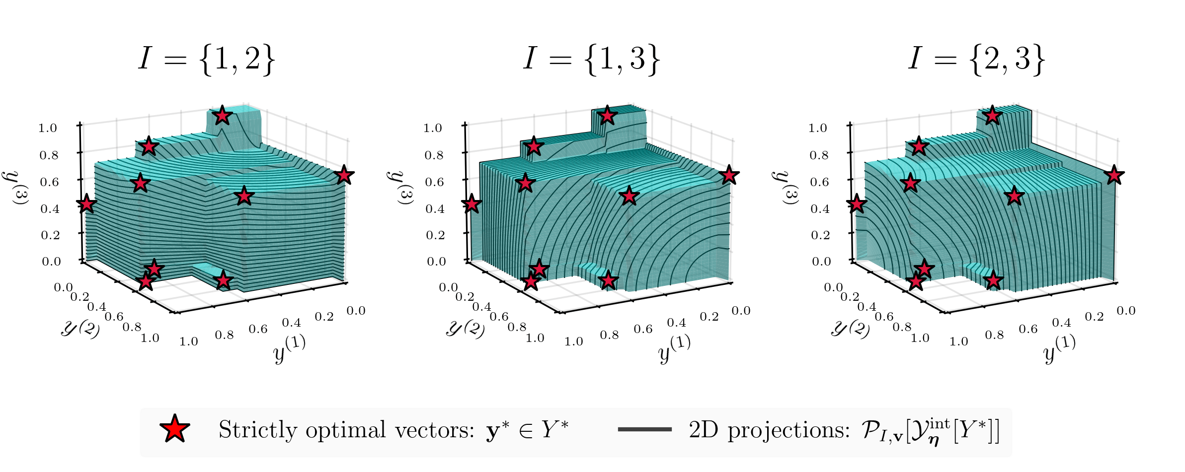
Figure 9: An illustration of the three different ways that we can generate two-dimensional slices of a three-dimensional Pareto front surface.

Projection mapping

We will now formalise the concept of the projected Pareto front surface, which is the natural extension to the ideas described above. To accomplish this, we define the reconstruction function $\phi_{I}:\mathcal{V}_{+}^{M-P}\times\mathcal{S}_{+}^{P-1}\rightarrow\mathcal{S}_{+}^{M-1}$, which creates a positive unit vector whose projected values are given by

$$\mathcal{P}_{I}(\phi_{I}(\mathbf{v},\boldsymbol{\lambda}))=\sqrt{1-||\mathbf{v}||_{L^{2}}^{2}}\boldsymbol{\lambda}\quad\text{ and }\quad\mathcal{P}_{[M]\setminus I}(\phi_{I}(\mathbf{v},\boldsymbol{\lambda}))=\mathbf{v}$$

for any non-empty set of $P$ ordered indices $I=\{i_{1},\dots,i_{P}\}\subset[M]$, any vector $\mathbf{v}\in\mathcal{V}_{+}^{M-P}$ and any positive unit vector $\boldsymbol{\lambda}\in\mathcal{S}_{+}^{P-1}$. Explicitly, the reconstruction function takes the form

$$\phi_{I}^{(m)}(\mathbf{v},\boldsymbol{\lambda}):=\begin{cases}\sqrt{1-||\mathbf{v}||_{L^{2}}^{2}}\lambda^{(p)},&\text{if }m\in I\text{ and }m=i_{p},\\ v^{(p)},&\text{if }m\in J\text{ and }m=j_{p},\end{cases}$$ (26)

for $m=1,\dots,M$, where $J=[M]\setminus I=\{j_{1},\dots,j_{M-P}\}$ denotes the complement of $I$ containing $M-P$ ordered indices. Using this function, we define the projection mapping $\mathcal{P}_{I,\mathbf{v}}:\mathbb{L}_{\boldsymbol{\eta}}\rightarrow\mathbb{L}_{\mathcal{P}_{I}(\boldsymbol{\eta})}$ to satisfy the equation

$$\begin{split}\mathcal{P}_{I,\mathbf{v}}[A]&:=\{\mathcal{P}_{I}(\boldsymbol{\eta})+\ell_{\boldsymbol{\eta},\phi_{I}(\mathbf{v},\boldsymbol{\lambda})}[A]\sqrt{1-||\mathbf{v}||_{L^{2}}^{2}}\boldsymbol{\lambda}\in\mathbb{R}^{P}:\boldsymbol{\lambda}\in\mathcal{S}_{+}^{P-1}\},\end{split}$$ (27)

for any polar surface $A\in\mathbb{L}_{\boldsymbol{\eta}}$. In Proposition 5.1, we show that the projection of any Pareto front surface $A^{*}\in\mathbb{Y}^{*}_{\boldsymbol{\eta}}$, that is $\mathcal{P}_{I,\mathbf{v}}[A^{*}]\in\mathbb{L}_{\mathcal{P}_{I}(\boldsymbol{\eta})}$, is a valid $P$-dimensional Pareto front surface with the reference vector $\mathcal{P}_{I}(\boldsymbol{\eta})\in\mathbb{R}^{P}$. This result follows similarly in spirit to Lemma 5.1. For completeness, we explicitly state this result below in Proposition 5.1 and prove it in Section A.8. In addition, we have also included a concrete example in Figure 9, where we demonstrate how a three-dimensional Pareto front surface can be partitioned into a collection of two-dimensional slices.

Proposition 5.1 (Projected Pareto front surface)

For any Pareto front surface $A^{*}\in\mathbb{Y}_{\boldsymbol{\eta}}^{*}$, any non-empty set of $P>0$ indices $I\subset[M]$, any vector $\mathbf{v}\in\mathcal{V}_{+}^{M-P}$, the corresponding projected Pareto front surface (27) is a $P$-dimensional Pareto front surface with the reference vector $\mathcal{P}_{I}(\boldsymbol{\eta})\in\mathbb{R}^{P}$, that is $\mathcal{P}_{I,\mathbf{v}}[A^{*}]\in\mathbb{Y}^{*}_{\mathcal{P}_{I}(\boldsymbol{\eta})}$.

Remark 5.1 (Non-constant fixed vector)

The projected Pareto front surface $\mathcal{P}_{I,\mathbf{v}}[A^{*}]\in\mathbb{Y}^{*}_{\mathcal{P}_{I}(\boldsymbol{\eta})}$ only considers the values indexed by the set $I$. It ignores the values at the other components $[M]\setminus I$. The values at these components were a constant for the spherical Pareto front surface $\mathcal{S}_{+}^{M-1}$, but there are not necessarily a constant for a general Pareto front surface $A^{*}\in\mathbb{Y}_{\boldsymbol{\eta}}^{*}$. Specifically, the projected vector at these indices are given by

$$\mathcal{P}_{[M]\setminus I}(\boldsymbol{\eta})+\ell_{\boldsymbol{\eta},\phi_{I}(\mathbf{v},\boldsymbol{\lambda})}[A^{*}]\mathbf{v}\in\mathbb{R}^{M-P}$$

for any $\boldsymbol{\lambda}\in\mathcal{S}_{+}^{P-1}$. Note that this vector is constant if and only if the projected lengths $\ell_{\boldsymbol{\eta},\phi_{I}(\mathbf{v},\boldsymbol{\lambda})}[A^{*}]$ are constant for all $\boldsymbol{\lambda}\in\mathcal{S}_{+}^{P-1}$. If this is not the case, then one must also be aware of this feature when examining the slices.

5.1.2 One-dimensional projection

The polar parametrisation result gives us a way to navigate a Pareto front surface by simply navigating the space of unit vectors $\boldsymbol{\lambda}\in\mathcal{S}_{+}^{M-1}$. We made a simple dashboard application to illustrate how such a navigation can be done in practice. We give a snapshot of this application in Figure 10. Below we describe the main concept of this application.

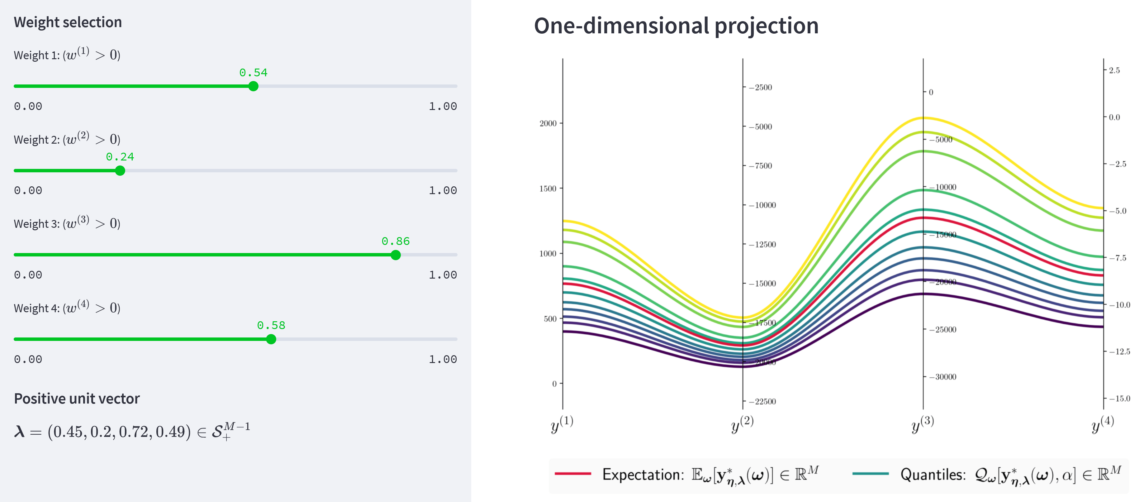
Figure 10: An illustration of the dashboard application that we made in order to navigate the space of one-dimensional projections of a Pareto front surface (Section 5.1.2).

Weights

We can navigate the space of unit vectors by moving $M$ different sliders. Each slider is associated with a weight lying in the open unit interval: $w^{(m)}\in(0,1)$ for the objectives $m=1,\dots,M$. The positive unit vector can then be constructed by normalising the weight vector appropriately: $\boldsymbol{\lambda}=\mathbf{w}/||\mathbf{w}||_{L^{2}}\in\mathcal{S}_{+}^{M-1}$.

Normalisation

Ideally, we want the weight vector $\mathbf{w}\in(0,1)^{M}$ to denote the relative importance of each objective. For this reason, we apply a normalisation transformation $\tau:\mathbb{R}^{M}\rightarrow\mathbb{R}^{M}$ to the objective vectors: $\tau(\mathbf{y})=(\mathbf{y}-\mathbf{l})/(\mathbf{u}-\mathbf{l})$ for any vector $\mathbf{y}\in\mathbb{R}^{M}$, where $\mathbf{l},\mathbf{u}\in\mathbb{R}^{M}$ denote the estimates for the lower and upper bound of the objective vectors, respectively. In addition, we also use these bound estimates to set the reference vector: $\boldsymbol{\eta}=\mathbf{l}-0.2(\mathbf{u}-\mathbf{l})\in\mathbb{R}^{M}$. As described in Remark 3.3, to reconstruct the Pareto front surface, we just have to invert this affine transformation, namely we set

$$\mathbf{y}^{*}_{\boldsymbol{\eta},\boldsymbol{\lambda}} =\tau^{-1}(\tau(\boldsymbol{\eta})+\ell_{\tau(\boldsymbol{\eta}),\boldsymbol{\lambda}}[\tau(A^{*})]\boldsymbol{\lambda})=\boldsymbol{\eta}+\ell_{\boldsymbol{\eta},\mathbf{r}}[A^{*}]\mathbf{r}\in\mathbb{R}^{M}$$

for all $\boldsymbol{\lambda}\in\mathcal{S}_{+}^{M-1}$, where $A^{*}\in\mathbb{Y}^{*}_{\boldsymbol{\eta}}$ is the Pareto front surface of interest and $\mathbf{r}\in\mathcal{S}_{+}^{M-1}$ denotes the updated positive unit vector with $r^{(m)}\propto(u^{(m)}-l^{(m)})\lambda^{(m)}$ for objectives $m=1,\dots,M$.

Parallel coordinates

To visualise the one-dimensional projections of the Pareto front surface, we propose using a parallel coordinates plot, which is a common visualisation tool for high-dimensional Pareto fronts (Tušar and Filipič, 2015). The novelty of our work is that we can also view uncertainty information along each projection as well. For example, in our application we computed and visualised the empirical quantiles and the sample mean obtained using a finite set of samples $\{A^{*}(\boldsymbol{\omega}_{n})\in\mathbb{Y}^{*}_{\boldsymbol{\eta}}\}_{n=1,\dots,N}$. Notably, this overall application is very lightweight to run because all of these statistics can computed and updated very quickly and cheaply on the fly.

5.1.3 Two-dimensional projection

Proposition 5.1 gives us a way to visualise a high-dimensional Pareto front surface by constructing a collection of low-dimensional slices that can be easily visualised instead. To illustrate how one might do this in practice, we created a simple dashboard application that can be used to navigate the set of two-dimensional slices of a Pareto front surface. We give a snapshot of this application in Figure 11. Below we describe the main concept of this application.

Indices and weights

To select the two indices $I=\{i_{1},i_{2}\}$, we used two drop-down lists. The corresponding fixed vector $\mathbf{v}\in\mathcal{V}_{+}^{M-2}$ is then determined by some weight sliders.

Normalisation

Similar to the one-dimensional application, we use an estimate of the objective ranges in order to normalise the objective values and set the reference vector.

Line plot

To visualise the two-dimensional projection of the Pareto front surface, we considered using a regular two-dimensional line plot. In our application, we included visuals on the empirical quantiles and the sample mean of the projected two-dimensional Pareto front surface. Naturally, other useful information could be included as well. For example, to address Remark 5.1, it might be beneficial to also include a parallel coordinates plot of the fixed vector as well—similar to the one used in Figure 10, but only for the fixed components.

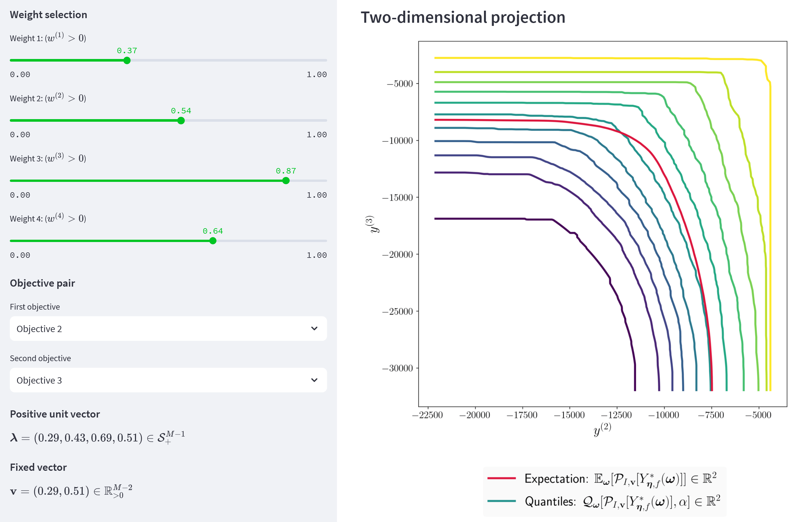
Figure 11: An illustration of the dashboard application that we made in order to navigate the space of two-dimensional projections of a Pareto front surface (Section 5.1.3).

5.1.4 Higher dimensional projections

In the previous sections, we have shown how it is possible to view a random Pareto front surface using one-dimensional or two-dimensional slices. The one-dimensional slices gave us information about the marginal performance for each objective. Whilst the two-dimensional slices gave us information about the correlation between any two objectives. Similarly, in order to learn more about the $P$-th order interactions, we need to be able to visualise the $P$-dimensional slices of the Pareto front surface. For example, one might consider adapting one of the methods surveyed by Tušar and Filipič (2015) in order to accomplish this.

5.2 Uncertainty quantification

The statistical concepts described in Section 4 gives us a tangible and useful way to analyse and quantify the uncertainty surrounding a distribution of random Pareto front surfaces. In this section, we highlight some potential use cases for this machinery in a Bayesian experimental design setting. Formally, we consider the problem of identifying the Pareto front surface associated with some bounded vector-valued black-box objective function $g:\mathbb{X}\rightarrow\mathbb{R}^{M}$. We suppose that we have executed an experimental design procedure and have observed a collection of potentially noisy data points $\mathcal{D}_{T}=\{(\mathbf{x}_{1},\mathbf{y}_{1}),\dots,(\mathbf{x}_{T},\mathbf{y}_{T})\}\subset\mathbb{X}\times\mathbb{R}^{M}$. We then adopt a standard Bayesian set-up in which we assume a probabilistic prior on the objective function $p(g)$ and a likelihood on the observations $p(\mathcal{D}_{T}|g)$. These variables can then be used to compute a posterior distribution over the objective function, $p(g|\mathcal{D}_{T})\propto p(g)p(\mathcal{D}_{T}|g)$, and consequently over the Pareto front surface, $Y_{\boldsymbol{\eta},g}^{*}:=\mathcal{Y}_{\boldsymbol{\eta}}^{\text{int}}[\{g(\mathbf{x})\}_{\mathbf{x}\in\mathbb{X}}]$, as summarised in the following flow diagram:

$$p(g),p(\mathcal{D}_{T}|g)\xrightarrow[\text{posterior}]{}p(g|\mathcal{D}_{T})\xrightarrow[\text{Pareto front}]{}p(Y_{\boldsymbol{\eta},g}^{*}|\mathcal{D}_{T}).$$

We can then appeal to our earlier work in Section 4 in order to study this resulting Pareto front surface distribution. Precisely, we can associate the stochastic process $f:\mathbb{X}\times\Omega\rightarrow\mathbb{R}^{M}$, described in Section 4, with the sampling distribution induced by the latest posterior model: $f(\cdot,\boldsymbol{\omega})\sim p(g|\mathcal{D}_{T})$, where $\boldsymbol{\omega}\in\Omega$ is distributed according to $\mathbb{P}$. We can then analyse and evaluate the posterior Pareto front surface distribution $p(Y_{\boldsymbol{\eta},g}^{*}|\mathcal{D}_{T})$ by studying the corresponding polar parametrised stochastic process described in (10). To showcase how this overall routine works in practice, we present an illustrative example in Section 5.2.1, where we visualise the evolution of a Pareto front surface distribution during a run of Bayesian optimisation. Afterwards, in Section 5.2.2, we then demonstrate how this distributional information can be used in conjunction with the visualisation techniques described in Section 5.1 in order to help us make final decisions.

5.2.1 Bayesian optimisation

Bayesian optimisation is a popular strategy for black-box optimisation—see the book by Garnett (2023) for a recent overview on this topic. Notably, this experimental design strategy takes advantage of a probabilistic surrogate model in order to determine the best inputs to evaluate. As described above, we can easily take advantage of this probabilistic model in order to compute any Pareto front surface statistic of interest. Practically speaking, we envision that these statistics might be valuable for an active decision maker who is interested in adapting the Bayesian optimisation run for their own purposes. For instance, one might use these statistics in conjunction with the visualisation ideas described in Section 5.1 in order to visualise and better understand the evolution of the Pareto front surface distribution. Given this newfound understanding, a keen decision maker might then actively refine and reprogram the acquisition procedure in order to target a specific region of interest. Alternatively, earlier work by Binois et al. (2015a) suggested that it might also be possible to use some Pareto front surface statistics, such as the Vorob’ev deviation (22), as a basis for a stopping criteria.

In Figure 12, we illustrate an example of how the Pareto front surface distribution evolves over time during one run of the Bayesian optimisation algorithm applied on the Gaussian mixture model (GMM) (Daulton et al., 2022) and the DTLZ2 (Deb et al., 2002) benchmark problem. For the probabilistic model, we adopted a standard Gaussian process prior (Rasmussen and Williams, 2006) on our objective function and an independent Gaussian observation likelihood on the function observations. For the acquisition function, we used the expected hypervolume improvement (Emmerich et al., 2006). For illustrative convenience, we discretised the input space in both of these benchmark problems to have $|\mathbb{X}|=2^{12}$ points. This latter simplification is only to ensure that we can compute the Pareto front surface of the objective function and the model samples exactly using our polar parametrisation.

There are a number of key observations that we see from the plots in Figure 12. Firstly, we see that the Pareto front surface distribution does indeed slowly converge to the actual Pareto front surface when we observe more data points. This is clearly a desirable property and is something that is expected on these benchmark problems. Secondly, we see that the model Pareto front surface always dominates the sample Pareto front surface in these examples. This makes intuitive sense because the sample front considers only a finite number of $|Y_{T}|=T$ points. In contrast, the model Pareto front surface considers the objective values over the entire input space. Note however that this intuition only holds in our example because the observations were not contaminated with any output noise. Otherwise, when there is observation noise in our data, the sample Pareto front could easily dominate both the actual and model Pareto front surface. For this reason, it is common for practitioners to rely on model-based estimates of the Pareto front surface when the data is noisy. Thirdly, we see that the uncertainty of the Pareto front surface does not necessarily decrease in a monotonic fashion as we add more points. This feature naturally arises in our example because we did not fix the model hyperparameters in our Gaussian process prior. Instead, we followed standard practice and updated these hyperparameters in an online manner by always maximising the latest log marginal likelihood. As a result of this updating step, the overall uncertainty in the Pareto front surface occasionally increased when we incorporate more points—for instance we see this feature when we transition from $T=20$ to $T=30$ in the GMM problem.

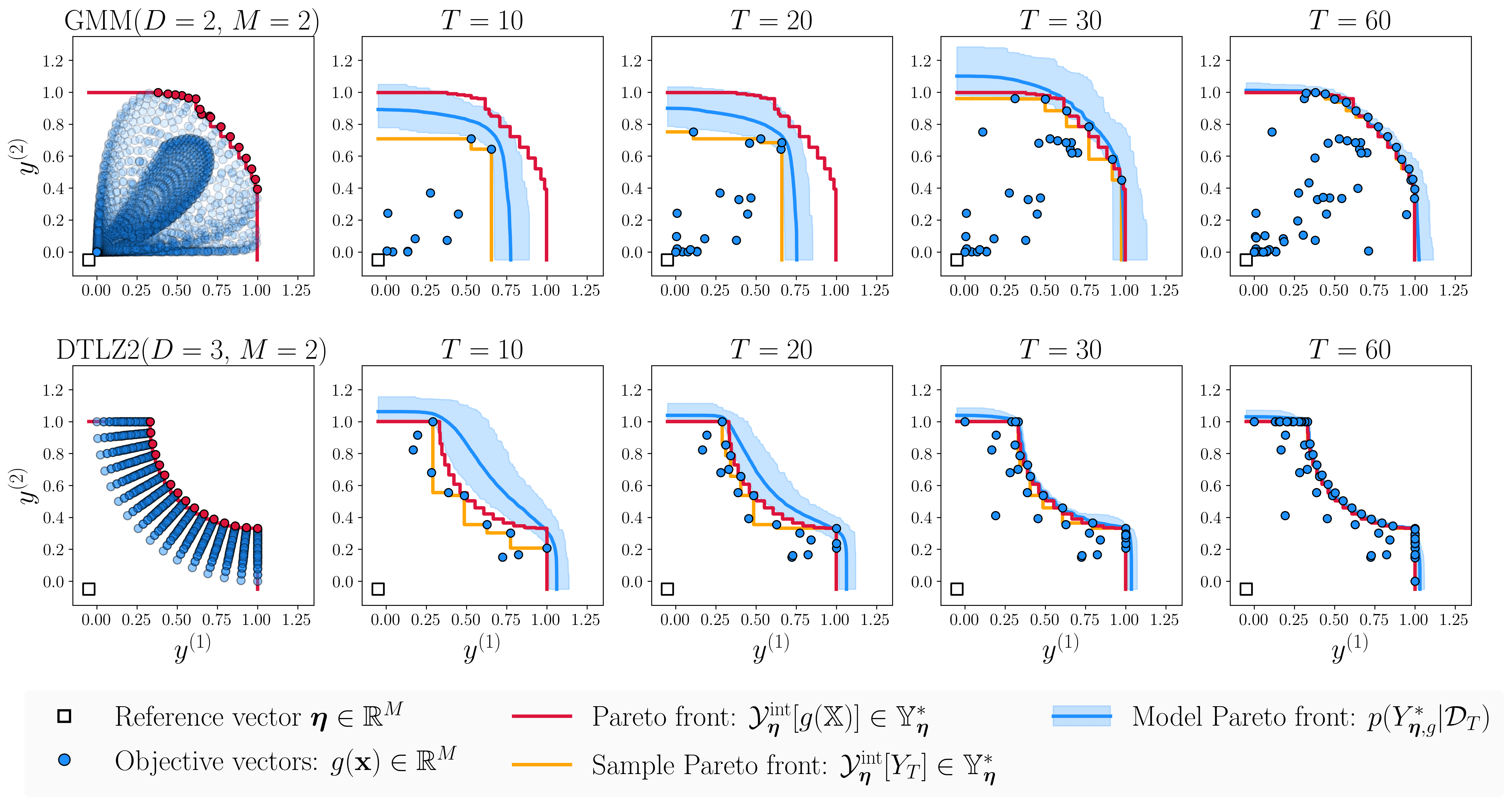
Figure 12: An illustration of the change in the Pareto front surface distribution $p(Y_{\boldsymbol{\eta},g}^{*}|\mathcal{D}_{T})$ when we perform Bayesian optimisation on the normalised GMM and DTLZ2 benchmarks. In the plots, we draw the estimated mean front and highlight the region between the $5\%$ and $95\%$ estimated quantile fronts.

5.2.2 Input decision

The Pareto front surface distribution gives us information on how the optimal set of objective vectors are distributed. This valuable information can be used by the decision maker in order to guide them in their downstream decision making. For instance, this information can help them decide which feasible objective vectors $\mathbf{y}^{*}\in\mathbb{R}^{M}$ are the most desirable. On a practical level, this post-selection procedure is typically handled with the help of an interactive application which allows the decision maker to visualise and navigate the Pareto front surface. Notably, we envision that the ideas and tools that we introduced earlier in Section 5.1 could be used in this interactive decision making procedure. Consequently, once the desirable vectors have been elicited, the decision maker would often be interested in identifying the inputs $\mathbf{x}^{*}\in\mathbb{X}$, which would most likely lead to these desirable vectors. To solve this problem, we propose adopting a decision-theoretic approach, where we select the best input as the one which minimise some $M$-dimensional loss function $L:\mathbb{R}^{M}\times\mathbb{R}^{M}\rightarrow\mathbb{R}$. That is, we propose minimising the expected empirical loss

$$\mathbf{x}^{*}\in\operatorname*{arg\,min}_{\mathbf{x}\in\mathbb{X}}\frac{1}{N}\sum_{n=1}^{N}L(f(\mathbf{x},\boldsymbol{\omega}_{n}),\mathbf{y}^{*}),$$

where $\boldsymbol{\omega}_{n}\in\Omega$ denotes some independent samples of the random parameter and $\mathbf{y}^{*}\in\mathbb{R}^{M}$ denotes the target vector of interest. Clearly there are many potential loss functions that we can choose in practice. Motivated the work so far, we propose using a length-based loss function because it is interpretable and leads to the desired result.

Length-based loss function

A natural candidate for the loss function would be a frontier loss function (8):

$$L(\mathbf{y},\mathbf{y}^{*})=\mathcal{D}_{\boldsymbol{\eta},S}[\mathcal{Y}^{\textnormal{int}}_{\boldsymbol{\eta}}[\{\mathbf{y}\}],\mathcal{Y}^{\textnormal{int}}_{\boldsymbol{\eta}}[\{\mathbf{y}^{*}\}]]$$

for any two vectors $\mathbf{y},\mathbf{y}^{*}\in\mathbb{R}^{M}$. A weakness of this loss function is that it can be very expensive to estimate and optimise in practice because it requires computing an integral over the space of positive unit vectors $\mathcal{S}_{+}^{M-1}$. Motivated by Lemma 3.1, we propose using a much cheaper simplification where we consider only computing the score along the optimal direction (3):

$$L(\mathbf{y},\mathbf{y}^{*})=S(s_{\boldsymbol{\eta},\boldsymbol{\lambda}_{\boldsymbol{\eta}}^{*}(\mathbf{y}^{*})}(\mathbf{y}),s_{\boldsymbol{\eta},\boldsymbol{\lambda}_{\boldsymbol{\eta}}^{*}(\mathbf{y}^{*})}(\mathbf{y}^{*})).$$ (28)

Geometrically, this loss function scores any vector $\mathbf{y}\in\mathbb{R}^{M}$ by computing its projected length along the reference line $L_{\boldsymbol{\eta},\boldsymbol{\lambda}_{\boldsymbol{\eta}}^{*}(\mathbf{y}^{*})}=\{\boldsymbol{\eta}+t\boldsymbol{\lambda}_{\boldsymbol{\eta}}^{*}(\mathbf{y}^{*}):t\in\mathbb{R}\}$ and then comparing it with the desired projected length. We illustrate the efficacy of this strategy for a two-dimensional example in Figure 13. We see clearly in this example that the random vectors $f(\mathbf{x}^{*},\boldsymbol{\omega})\in\mathbb{R}^{M}$ associated with the best inputs $\mathbf{x}^{*}\in\mathbb{X}$ are indeed distributed close to the corresponding target vectors $\mathbf{y}^{*}\in\mathbb{R}^{M}$.

Remark 5.2 (Scale sensitivity)

Any $M$-dimensional loss function will naturally be sensitive to the scales of the different objectives. When using the length-based loss functions (28), we recommend normalising each objective by its range in order for each objective to have a similar influence on the projected length as illustrated in Section 5.1.2. Evidently we can also take advantage of this sensitivity in order to inflate the importance of some objectives over others. That is, in order to up-weight the importance of an objective, we can increase its range and similarly in order to down-weight the importance of an objective, we can decrease its range.

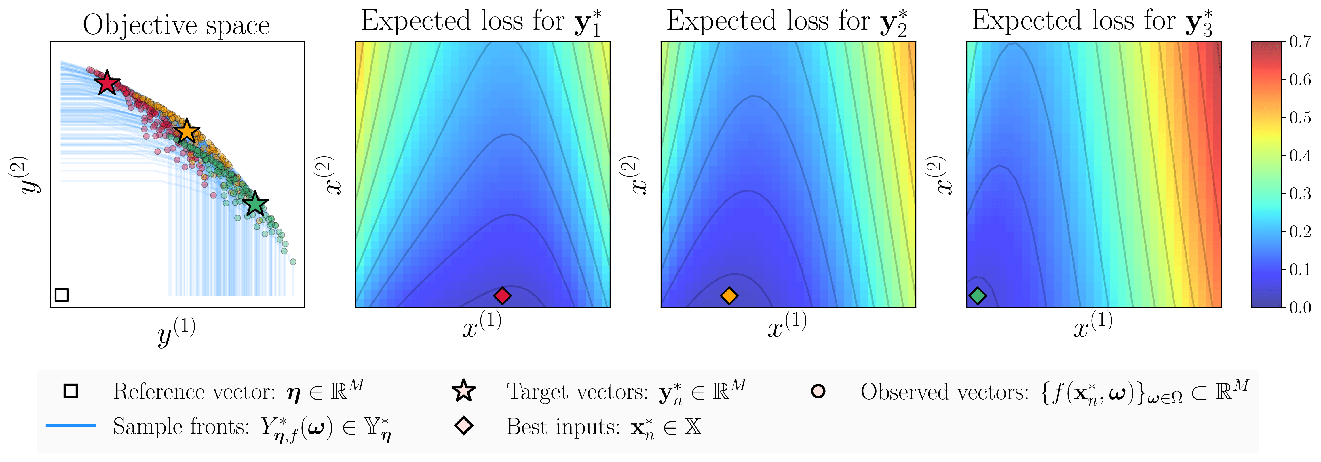
Figure 13: An illustration of the best input attained by minimising the length based loss function (28) with the squared error scoring function $S(x,y)=(x-y)^{2}$.

5.3 Extreme value theory

Extreme value theory is a well-established branch of statistics which studies the distribution of extreme values—see for instance Embrechts et al. (1997); Coles (2001) or Beirlant et al. (2004) for a background on this topic. In this section, we showcase how our polar parametrisation result can be used in order to generalise many existing ideas in this topic to the multivariate setting, where the maximum is defined using the Pareto partial ordering. To the best of our knowledge, the majority of existing work in multivariate extreme value theory has largely focussed on the marginal maximisation setting (Barnett, 1976), where the maximum operation on a set of vectors is defined component-wise. Much less work, if any, has focussed on the setting where the maximum is defined using the Pareto partial ordering. The clear benefit of this latter approach is that it is much more flexible in practice because it can accommodate for the scenario where the various component-wise maximums do not all take place simultaneously.

The most notable results from extreme value theory are the Fisher–Tippett–Gnedenko theorem (Fisher and Tippett, 1928; Gnedenko, 1943) and the Balkema–de Haan–Pickands theorem (Balkema and de Haan, 1974; Pickands, 1975). The former result is concerned with the asymptotic distribution of the maximum order statistic associated with a collection of independent and identically distributed univariate random variables. In words, it states that the distribution of the maximum, upon proper normalisation, can only converge in distribution to either a Gumbel, Fréchet or Weibull distribution. In contrast, the latter result is concerned with the limiting distribution of the corresponding conditional excess distribution (Definition 5.2). Conceptually, this result tells us that the distribution of the tail events, pass some threshold, can be closely approximated by a generalised Pareto distribution. For reference purposes, we repeat both of these results below in Theorem 5.1 and Theorem 5.2, respectively.

Definition 5.1 (Maximum domain of attraction)

A cumulative distribution function $F:\mathbb{R}\rightarrow\mathbb{R}$ is in the maximum domain of attraction (MDA) of a cumulative distribution function $H:\mathbb{R}\rightarrow\mathbb{R}$, denoted by $F\in\text{MDA}(H)$, if there exist two sequences of real numbers $a_{N}>0$ and $b_{N}\in\mathbb{R}$ such that

$$\lim_{N\rightarrow\infty}\mathbb{P}\biggl{[}\frac{\max(\{Y_{1},\dots,Y_{N}\})-b_{N}}{a_{N}}\leq x\biggr{]}=\lim_{N\rightarrow\infty}F(a_{N}x+b_{N})^{N}=H(x)$$

for $x\in\mathbb{R}$, where $Y,Y_{1},\dots,Y_{N}\in\mathbb{R}$ denotes a collection of independent and identically distributed random samples from the distribution $F$.

Theorem 5.1 (Extreme value distribution)

(Fisher and Tippett, 1928; Gnedenko, 1943) If the cumulative distribution function $F:\mathbb{R}\rightarrow\mathbb{R}$ is in the MDA of a non-degenerate distribution function $H:\mathbb{R}\rightarrow\mathbb{R}$, that is $F\in\text{MDA}(H)$, then $H(x)=\exp(-(1+\xi(\frac{x-\mu}{\sigma}))_{+}^{-1/\xi})$ is a generalised extreme value distribution, where $\xi\in\mathbb{R}$, $\mu\in\mathbb{R}$ and $\sigma>0$, denotes the shape, location and scale parameter, respectively.

Definition 5.2 (Conditional excess distribution)

Let $Y\in\mathbb{R}$ denote a random variable with a distribution function $F:\mathbb{R}\rightarrow\mathbb{R}$. The corresponding conditional excess distribution function at some level $u\in\mathbb{R}$ is given by

$$F_{u}(x):=\mathbb{P}[Y-u\leq x|Y>u]=\frac{F(u+x)-F(u)}{1-F(u)},$$

for any $x\in[0,y_{F}-u]$, where $y_{F}:=\sup\{x\in\mathbb{R}:F(x)<1\}$ denotes the finite or infinite right endpoint of the distribution function $F$.

Theorem 5.2 (Generalised Pareto distribution)

(Balkema and de Haan, 1974; Pickands, 1975) If the cumulative distribution function $F:\mathbb{R}\rightarrow\mathbb{R}$ is in the MDA of a generalised extreme value distribution, $F\in\text{MDA}(H_{\xi,\mu,\sigma})$, then there exists a positive, measurable function $\beta:\mathbb{R}\rightarrow\mathbb{R}_{>0}$ such that the following limit holds:

$$\lim_{u\rightarrow y_{F}}\sup_{x\in[0,y_{F}-u]}|F_{u}(x)-G_{\xi,\beta(u)}(x)|=0$$

where $G_{\xi,\beta}(x)=1-(1+\frac{\xi x}{\beta})_{+}^{-1/\xi}$ denotes the distribution function of a generalised Pareto distribution with shape parameter $\xi\in\mathbb{R}$ and rate parameter $\beta>0$.

Component-wise maximum

The existing work on multivariate extreme value theory has largely focussed on the marginal maximisation setting where the maximum of a collection of $N$ independent and identically-distributed vectors $Y_{1},\dots,Y_{N}\in\mathbb{R}^{M}$ are defined component-wise. The traditional goal of interest is then to study the multivariate generalisation of the MDA for the resulting multivariate distribution function $F:\mathbb{R}^{M}\rightarrow\mathbb{R}$,

$$F(\mathbf{x})=\mathbb{P}[\max(\{Y^{(1)}_{1},\dots,Y^{(1)}_{N}\})\leq x^{(1)},\dots,\max(\{Y^{(M)}_{1},\dots,Y^{(M)}_{N}\})\leq x^{(M)}]$$

for $\mathbf{x}\in\mathbb{R}^{M}$—see Beirlant et al. (2004, Chapter 8) for an overview on this topic. The primary benefit of using this component-wise definition is that we can immediately apply both Theorem 5.1 and Theorem 5.2 in order to determine the asymptotic properties of the corresponding marginal distributions. The remaining challenge is then to identify the corresponding dependence structure between the components. This latter problem turns out to be a major hurdle in multivariate extreme value theory because this dependency structure cannot necessarily be described using a finitely parametrised model. Notably, the estimation and analysis of this dependency structure is still an area of active research—see Beirlant et al. (2004, Chapter 8) for an in-depth discussion.

Pareto maximum

To the best of our knowledge, there does not exist much work regarding the study of multivariate extreme value theory when we use the Pareto definition of the vector-valued maximum (Definition 2.4). We attribute this lack of interest based on the fact that the Pareto maximum is very challenging to work with in practice. One remarkable outcome of our work is that it manages to connect the definition of the Pareto maximum with the definition of the component-wise maximum. Specifically, our polar parametrisation result tells us that the Pareto maximum can be completely characterised by its projected length process (11), which is defined as an infinite collection of scalarised maximums. To put it more concretely, if we had a collection of identically-distributed vectors $Y_{1},\dots,Y_{N}\in\mathbb{R}^{M}$, then the corresponding Pareto maximum is governed by the following projected length process

$$\mathcal{L}_{\boldsymbol{\eta}}=\{\max(\{s_{\boldsymbol{\eta},\boldsymbol{\lambda}}(Y_{1}),\dots,s_{\boldsymbol{\eta},\boldsymbol{\lambda}}(Y_{N})\})\geq 0:\boldsymbol{\lambda}\in\mathcal{S}^{M-1}_{+}\}$$

for any reference vector $\boldsymbol{\eta}\in\mathbb{R}^{M}$. As a consequence of this observation, many of the results that are known for the component-wise maximum can now be adapted to the Pareto maximum setting. For example, we can use Theorem 5.1 to determine the possible asymptotic distributions of the projected length process along each positive direction. Similarly, we can use Theorem 5.2 in order to approximate the distribution of the tails of the projected length process conditional on the fact that it dominates some specified polar surface. That is, instead of setting just a single threshold value of $u\in\mathbb{R}$, we set the threshold to be a polar surface defined by some set $\mathcal{U}=\{u_{\boldsymbol{\lambda}}\geq 0:\boldsymbol{\lambda}\in\mathcal{S}^{M-1}_{+}\}$.

As a proof of concept for these general ideas, we present a simple example in Proposition 5.2, where we study the asymptotic distribution of a Pareto front surface constructed using a collection of independent Weibull distributed vectors. Formally, this result states that, upon proper normalisation, the projected length process of this Pareto front surface distribution converges in distribution to a Gumbel distribution along each positive direction—the proof of this result is presented in Section A.11. To illustrate this convergence, we present some visual two-dimensional examples in Figure 14. In these plots, we fixed the rate parameter $\beta^{(m)}>0$ and varied the choice of shape parameter $\alpha>0$. On the whole, we see that the empirical and limiting distributions are already quite similar even at small sample sizes such as $N=64$. Conceptually, we see that varying the shape parameter $\alpha>0$ amounts to changing from a concave Pareto front surface distribution when $\alpha\in(0,1)$ to a convex Pareto front surface distribution when $\alpha>1$.

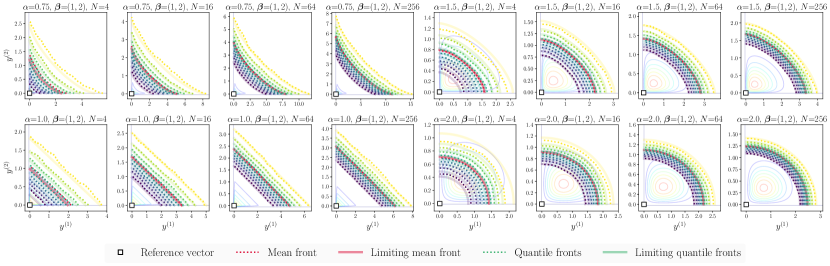
Figure 14: An illustration of the Pareto front surface statistics associated with a collection of independent Weibull distributions (Proposition 5.2). In the dotted lines, we plot the empirical estimates obtained using $N\in\{4,16,64,256\}$ random samples, whereas in the shaded lines we plot the predicted mean and quantiles given by the limiting distribution. As a reference, we also plot the contour of the corresponding bivariate probability density function as well.

Proposition 5.2 can also be used in conjunction with Theorem 5.2. In words, this result tells us that the tails of the corresponding projected length process are approximately distributed according to an exponential distribution. To demonstrate this property, we present an illustrative example in Figure 15, where we study the conditional excess probabilities associated with the $M=2$ dimensional Pareto front surface distributions described in Figure 14. That is, we plot the probabilities

$$F_{\mathcal{U}}(\mathbf{z}):=\mathbb{P}[s_{\boldsymbol{\eta},\boldsymbol{\lambda}_{\boldsymbol{\eta}}^{*}(\mathbf{z})}(Y)-u_{\boldsymbol{\lambda}_{\boldsymbol{\eta}}^{*}(\mathbf{z})}\leq s_{\boldsymbol{\eta},\boldsymbol{\lambda}_{\boldsymbol{\eta}}^{*}(\mathbf{z})}(\mathbf{z})|s_{\boldsymbol{\eta},\boldsymbol{\lambda}_{\boldsymbol{\eta}}^{*}(\mathbf{z})}(Y)>u_{\boldsymbol{\lambda}_{\boldsymbol{\eta}}^{*}(\mathbf{z})}]$$ (29)

for any $\mathbf{z}\in\mathbb{D}_{\succ\mathrel{\mkern-5.0mu}\succ}[\{\boldsymbol{\eta}\}]$, where $\boldsymbol{\eta}=\mathbf{0}_{M}$ is the reference vector, $Y\in\mathbb{R}^{M}$ is the random vector of interest and $\mathcal{U}=\{u_{\boldsymbol{\lambda}}\geq 0:\boldsymbol{\lambda}\in\mathcal{S}^{M-1}_{+}\}$ is the projected length process which defines the threshold polar surface. For convenience, in these examples, we set the threshold polar surface to be one of upper quantiles. Nevertheless, we note that any polar surface, whose projected length process is sufficiently long, can be used in practice. Overall we see that these empirical estimates are indeed close to their theoretical approximate values.

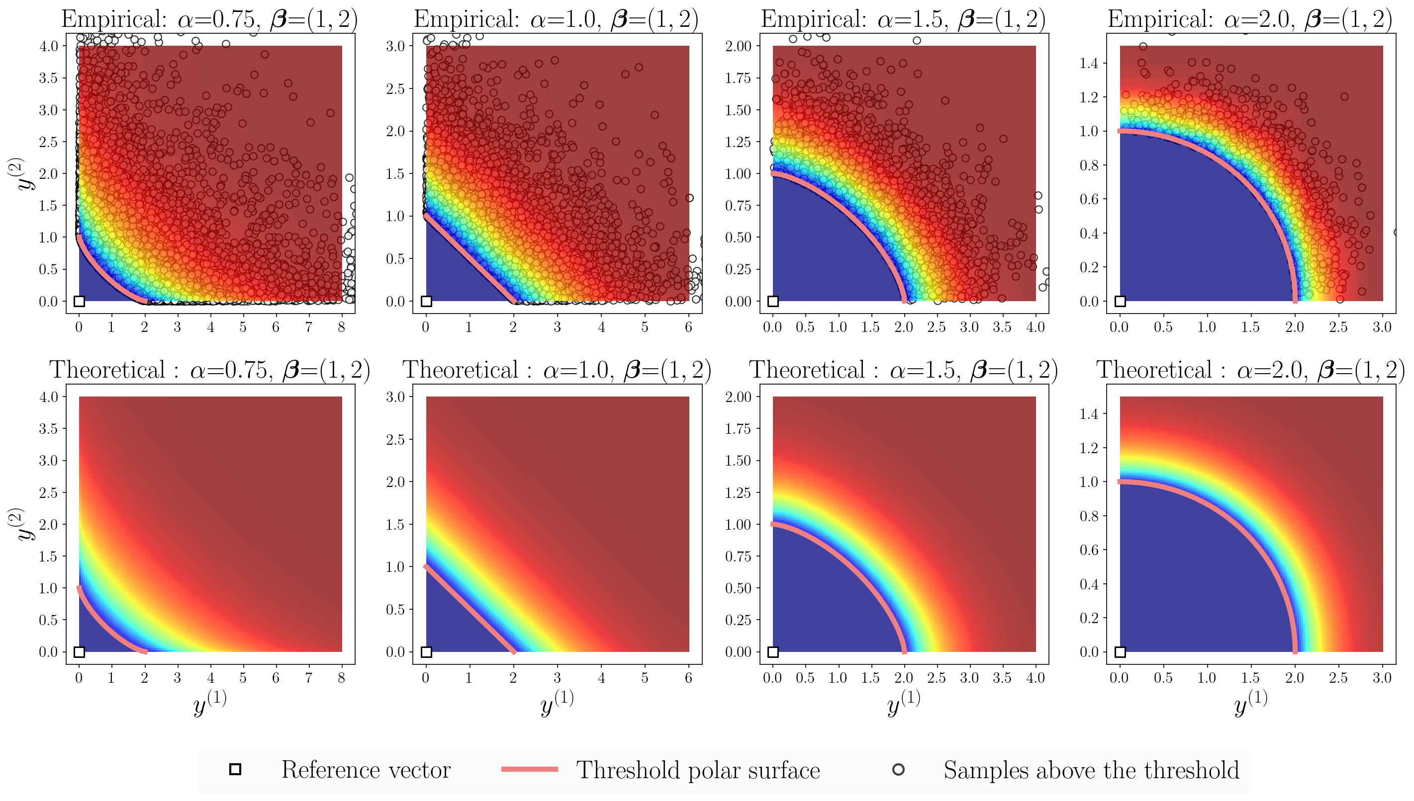
Figure 15: A comparison between the empirical and theoretical approximation of the conditional excess probabilities (29) associated with the two-dimensional Pareto front surface distributions described in Figure 14. To set the threshold polar surface, we used an upper quantile of the original Pareto front surface distribution.

Proposition 5.2 (Weibull distributed vectors)

Let the reference vector be set to zero $\boldsymbol{\eta}=\mathbf{0}_{M}\in\mathbb{R}^{M}$ and the vectors $Y_{n}\in\mathbb{R}^{M}$ be distributed according to $M>0$ independent Weibull distributions,

$$Y_{n}^{(m)}\sim\textnormal{Weibull}(\alpha,\beta^{(m)}),$$

with the cumulative distribution function $\mathbb{P}[Y^{(m)}\leq x]=1-\exp(-(\beta^{{(m)}}x)^{\alpha})$, where $\alpha>0$ and $\beta^{(m)}>0$ denotes the corresponding the shape and rate parameter for $m=1,\dots,M$, respectively. Then, upon proper normalisation, the projected lengths of $\mathcal{Y}_{\boldsymbol{\eta}}^{\textnormal{int}}[\{Y_{1},\dots,Y_{N}\}]$, along any positive direction $\boldsymbol{\lambda}\in\mathcal{S}^{M-1}_{+}$, converges to a standard Gumbel distribution:

$$\lim_{N\rightarrow\infty}\mathbb{P}\biggl{[}\frac{\ell_{\boldsymbol{\eta},\boldsymbol{\lambda}}[\mathcal{Y}_{\boldsymbol{\eta}}^{\textnormal{int}}[\{Y_{1},\dots,Y_{N}\}]]-b_{\boldsymbol{\eta},\boldsymbol{\lambda},N}}{a_{\boldsymbol{\eta},\boldsymbol{\lambda},N}}\leq x\biggr{]}=\exp(-\exp(-x))$$

where $a_{\boldsymbol{\eta},\boldsymbol{\lambda},N}=\log(N)^{1/\alpha-1}/(\alpha k_{\boldsymbol{\lambda}})$, $b_{\boldsymbol{\eta},\boldsymbol{\lambda},N}=\log(N)^{1/\alpha}/k_{\boldsymbol{\lambda}}$ and $k_{\boldsymbol{\lambda}}=(\sum_{m=1}^{M}(\beta^{{(m)}}\lambda^{(m)})^{\alpha})^{1/\alpha}$.

Remark 5.3 (Endpoint estimation)

As identified by Binois et al. (2015b), the Pareto front surface of an objective function $g:\mathbb{X}\rightarrow\mathbb{R}^{M}$ can also be viewed as the uppermost quantile of a Pareto front surface distribution (Binois et al., 2015b, Theorem 2.1),

$$\mathcal{Y}_{\boldsymbol{\eta}}^{\textnormal{int}}[\{g(\mathbf{x})\}_{\mathbf{x}\in\mathbb{X}}]=\lim_{\alpha\rightarrow 1}\mathcal{Q}_{\mathbf{x}\sim p(\mathbf{x})}[\mathcal{Y}_{\boldsymbol{\eta}}^{\textnormal{int}}[\{g(\mathbf{x})\}],\alpha],$$

where $p(\mathbf{x})\geq 0$ denotes the density of any distribution over the input space whose essential support covers the entire input space; for instance, a uniform distribution over $\mathbb{X}$. As emphasised by Binois et al. (2015b), the clear benefit of this result is that it transforms the vector-valued optimisation problem into an endpoint estimation problem. This latter topic is naturally related with extreme value theory (Hall, 1982; Loh, 1984; Girard et al., 2012).

5.4 Air pollution example

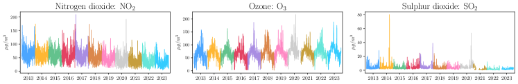
Figure 16: An illustration of the daily maximum registered pollutants at the North Kensington monitoring station (UKA00253) over the period of 2013 to 2023.

Figure 17: An illustration of the change in the domination probabilities for the pairwise Pareto front surfaces associated with the air pollution data (Figure 16).

The previous examples shown in this work have largely been focussed on static problems which have no time dependency. Nevertheless, all of the ideas that we have presented so far can also accommodate for dynamic problems, where there is indeed some time dependency. As an illustrative example, we will now consider how these ideas can be used on a real-world time series data set. Precisely, we study the air pollution data obtained at the North Kensington (UKA00253) air monitoring station in west London.

Data cleaning

The air monitoring station at North Kensington measures many different pollutants every day at different frequencies. We focus our attention on the measurements on the three key pollutants in this area: Nitrogen dioxide $(\text{NO}_{2})$, Ozone $(\text{O}_{3})$ and Sulphur dioxide $(\text{SO}_{2})$. The Nitrogen dioxide and Ozone are measured at a rate of once every $60$ minutes, whilst the Sulphur dioxide is measured at a rate of once every $15$ minutes. In our work, we use the daily maximum of the measured observations as our statistic of interest. Sometimes there are periods where some subset of the measurement devices are offline and therefore no readings can be made. The daily maximums are then computed by using the partial observations that were recorded. On the days where no observations were made at all, we omit the day entirely. In Figure 16, we plot the resulting time series of these daily maximums over the period of 2013 to 2023.

Pareto front surface distributions

In this working example, we assume that the goal of interest is to assess and better understand the change in the daily worst-case Pareto front surface of pollution in the North Kensington area over the last decade. That is, we want to see the change in the Pareto fronts of the daily maximum pollutants over the different years. Practically speaking, we envision that this information might be useful for policy makers who are interested in assessing the effectiveness of new pollution reducing initiatives in London such as the Ultra Low Emission Zone (ULEZ) or the lowering of the local speed limits. In Figure 17, we take advantage of some of our Pareto front machinery in order to compute and plot the corresponding domination probabilities for the different pairwise Pareto front surfaces. We see clearly that there is a general positive trend after 2020, where the Pareto front has been progressing downwards. This indicates a general reduction in the daily maximum pollution. Evidently this time period also aligns with many events such as: the Coronovirus pandemic, the introduction of ULEZ and the lowering of local speed limits. Cumulatively, all of these effects seem to have had a noticeably positive impact on reducing the daily maximum detected Nitrogen dioxide and Sulphur dioxide in North Kensington. Nevertheless, the maximum amount of Ozone is still at a comparative level to the earlier years. To further illustrate the reduction of these domination probabilities more explicitly, we plot and calculate the corresponding average yearly signed changes in Figure 18. That is, we compare every year’s Pareto front surface distribution with the previous year and see where the relative positive and negative changes occur. On the whole, we see that there is indeed a quantifiable reduction happening over the later years as these new initiatives were being introduced.

Figure 18: An illustration of the signed yearly changes in the domination probabilities for the pairwise Pareto fronts described in Figure 17. The average yearly negative and positive changes are depicted in the legends. The total average yearly change can be computed by summing the absolute values of these signed changes.

6 Conclusion

In this work we have studied the space of Pareto front surfaces. We presented a novel result which showed that any Pareto front surface can be explicitly parametrised using polar coordinates. We then used this polar parametrisation result in order to establish many general concepts over the space of Pareto front surfaces. Notably, we focussed our attention on the stochastic setting where the Pareto front surface itself was random. We showed that this random surface admits a stochastic process representation (10), based on our polar parametrisation, which makes it amenable to standard ideas from functional data analysis. In particular, we used this stochastic representation in order to define and compute statistics for random Pareto front surfaces. We then demonstrated the usefulness of these new probabilistic ideas on some interesting applications such as: visualisation, uncertainty quantification and extreme value theory. In the following paragraphs, we highlight some interesting directions for future research.

Other interpolation schemes

Throughout this work, we have focussed our attention on the interpolated Pareto front (Definition 2.4), which was defined using the weak Pareto partial ordering. This type of interpolation is sensible because it is consistent with the weak Pareto partial ordering on sets (Definition 3.2): $\mathcal{Y}_{\boldsymbol{\eta}}^{\text{int}}[A]\preceq\mathcal{Y}_{\boldsymbol{\eta}}^{\text{int}}[B]$ if $A\subseteq B\subseteq\mathbb{D}_{\succ\mathrel{\mkern-5.0mu}\succ}[\{\boldsymbol{\eta}\}]$. In practice, one might also consider using alternate interpolation (or approximation) schemes such as the ones based on Delaunay triangulation (Hartikainen et al., 2012), sandwiching (Bokrantz and Forsgren, 2013) or hyperboxing (Dächert and Teichert, 2020; Eichfelder and Warnow, 2022). Notably these other schemes might be beneficial when we are interested in approximating a Pareto front of a continuous set $Y\subset\mathbb{R}^{M}$ using a finite subset $\hat{Y}\subseteq Y$. In this setting, the interpolated weak Pareto front of $\hat{Y}$ would always give us a lower bound estimate of the actual front. In contrast, a different interpolation scheme might be able to give us a more accurate approximation of the target front, with respect to some frontier loss (Section 3.3). Naturally, many of the results which we have shown here continues to hold even when we change the interpolation scheme. The only notable difference is that the corresponding projected length function $\ell_{\boldsymbol{\eta},\boldsymbol{\lambda}}$, which arises in the polar parametrisation (Theorem 3.1), might no longer be written in terms of the length scalarisation function (2). Instead, the new projected length function would likely depend on a different scalarisation function—one which accurately caters for the interpolation scheme at hand. We leave the analysis of these other interpolation schemes for future research.

Constrained regression

Our polar parametrisation result implies that any Pareto front surface is completely characterised by its projected length function. Whilst our result in Proposition 3.1 gives two necessary and sufficient conditions that a length function must satisfy in order for it to induce a valid Pareto front surface. An interesting direction for future work would be focussed on learning this projected length function directly from observational data. Note that the first constraint (C1), positivity, can be easily handled by just considering the logarithm of the length function instead. Whilst the second constraint (C2), the maximum ratio condition, is much less trivial to work with. Specifically, by taking the logarithm and rearranging the terms, we see that this latter condition is very similar to a Lipschitz type constraint, which is known to be challenging to work with.

Advancing the theory

Many of the ideas that we have established in this work can be generalised and adapted even further. For instance, we only exploited a few basic ideas from functional data analysis in order to define the Pareto front surface statistics in Section 4. Other ideas such as functional regression and functional principal component analysis were not explored in any detail and could be investigated in the future. Similarly, in Section 5.3, we gave a proof of concept on how one could extend well-known results from extreme value theory to work in the multivariate setting under the Pareto maximum. A practical direction for future work could focus on pushing these preliminary ideas even further.

Appendix A Proofs

We now prove all the results discussed in the main paper. Some of these proofs rely on the monotonicity of the length scalarisation function (2), which we define below. The proof of these monotonicity results follow immediately from the definition of the length scalarisation function for a fixed reference vector $\boldsymbol{\eta}\in\mathbb{R}^{M}$.

Lemma A.1 (Monotonically increasing)

The length scalarisation function is a monotonically increasing function over the whole of $\mathbb{R}^{M}$, that is $\mathbf{y}\succeq\mathbf{y}^{\prime}\implies s_{\boldsymbol{\eta},\boldsymbol{\lambda}}(\mathbf{y})\geq s_{\boldsymbol{\eta},\boldsymbol{\lambda}}(\mathbf{y}^{\prime})$ for all vectors $\mathbf{y},\mathbf{y}^{\prime}\in\mathbb{R}^{M}$ and any positive unit vector $\boldsymbol{\lambda}\in\mathcal{S}_{+}^{M-1}$.

Lemma A.2 (Strongly monotonically increasing)

The length scalarisation function is a strongly monotonically increasing function over the truncated space, that is $\mathbf{y}\succ\mathrel{\mkern-5.0mu}\succ\mathbf{y}^{\prime}\implies s_{\boldsymbol{\eta},\boldsymbol{\lambda}}(\mathbf{y})>s_{\boldsymbol{\eta},\boldsymbol{\lambda}}(\mathbf{y}^{\prime})$ for all vectors $\mathbf{y},\mathbf{y}^{\prime}\in\mathbb{D}_{\succ\mathrel{\mkern-5.0mu}\succ}[\{\boldsymbol{\eta}\}]$ and any positive unit vector $\boldsymbol{\lambda}\in\mathcal{S}_{+}^{M-1}$.

A.1 Proof of Theorem 3.1

Consider a bounded set of vectors $A\subset\mathbb{R}^{M}$ and reference vector $\boldsymbol{\eta}\in\mathbb{R}^{M}$ which admits a non-empty Pareto front surface $\mathcal{Y}_{\boldsymbol{\eta}}^{\textnormal{int}}[A]\neq\emptyset$. Let

$$A^{*}=\{\boldsymbol{\eta}+\sup_{\mathbf{y}\in A}s_{\boldsymbol{\eta},\boldsymbol{\lambda}}(\mathbf{y})\boldsymbol{\lambda}\in\mathbb{R}^{M}:\boldsymbol{\lambda}\in\mathcal{S}_{+}^{M-1}\}\in\mathbb{L}_{\boldsymbol{\eta}}.$$

We will first show that this polar surface contains the Pareto front surface: $\mathcal{Y}_{\boldsymbol{\eta}}^{\textnormal{int}}[A]\subseteq A^{*}$. To prove this result, we take advantage of the well-known fact that every Pareto optimal point $\mathbf{y}^{*}\in\mathcal{Y}_{\boldsymbol{\eta}}^{\textnormal{int}}[A]$ can be obtained by solving the following optimisation problem (Miettinen, 1998, Part 2, Theorem 3.4.5):

$$\mathbf{y}^{*}\in\operatorname*{arg\,max}_{\mathbf{y}\in\mathcal{Y}_{\boldsymbol{\eta}}^{\textnormal{int}}[A]}s^{\textnormal{Len}}_{(\boldsymbol{\eta},\boldsymbol{\lambda}^{*}_{\boldsymbol{\eta}}(\mathbf{y}^{*}))}(\mathbf{y})=\operatorname*{arg\,max}_{\mathbf{y}\in\mathcal{Y}_{\boldsymbol{\eta}}^{\textnormal{int}}[A]}\min_{m=1,\dots,M}\frac{y^{(m)}-\eta^{(m)}}{(y^{*})^{(m)}-\eta^{(m)}}.$$ (30)

From the monotonicity of the length scalarisation function (Lemma A.1), we have that

$$\max_{\mathbf{y}\in\mathcal{Y}_{\boldsymbol{\eta}}^{\textnormal{int}}[A]}s_{\boldsymbol{\eta},\boldsymbol{\lambda}}(\mathbf{y})=\sup_{\mathbf{y}\in\mathbb{D}_{\preceq,\boldsymbol{\eta}}[A]}s_{\boldsymbol{\eta},\boldsymbol{\lambda}}(\mathbf{y})=\sup_{\mathbf{y}\in A}s_{\boldsymbol{\eta},\boldsymbol{\lambda}}(\mathbf{y})$$

for any $\boldsymbol{\lambda}\in\mathcal{S}_{+}^{M-1}$. Combining this result with (30), we find that

$$\mathbf{y}^{*} =\mathcal{T}^{-1}_{\boldsymbol{\eta}}((\boldsymbol{\lambda}^{*}_{\boldsymbol{\eta}}(\mathbf{y}^{*}),s_{\boldsymbol{\eta},\boldsymbol{\lambda}_{\boldsymbol{\eta}}^{*}(\mathbf{y}^{*})}(\mathbf{y}^{*})))=\boldsymbol{\eta}+\sup_{\mathbf{y}\in A}s_{\boldsymbol{\eta},\boldsymbol{\lambda}_{\boldsymbol{\eta}}^{*}(\mathbf{y}^{*})}(\mathbf{y})\boldsymbol{\lambda}^{*}_{\boldsymbol{\eta}}(\mathbf{y}^{*})\in A^{*}$$

for all $\mathbf{y}^{*}\in\mathcal{Y}_{\boldsymbol{\eta}}^{\textnormal{int}}[A]$, which implies the desired result: $\mathcal{Y}_{\boldsymbol{\eta}}^{\textnormal{int}}[A]\subseteq A^{*}$. We will now show by a simple proof by contradiction that the other containment also holds: $\mathcal{Y}_{\boldsymbol{\eta}}^{\textnormal{int}}[A]\supseteq A^{*}$. Suppose for a contradiction that there exists a vector $\mathbf{a}^{*}\in A^{*}$ which is not Pareto optimal, that is $\mathbf{a}^{*}\notin\mathcal{Y}_{\boldsymbol{\eta}}^{\textnormal{int}}[A]$. Then by the definition of weak Pareto optimality (Definition 2.4), there must exist an element $\mathbf{y}^{*}\in A$ which strongly dominates it. As the length scalarisation function is strongly monotonically increasing over the truncated space (Lemma A.2), this implies that $s_{\boldsymbol{\eta},\boldsymbol{\lambda}}(\mathbf{y}^{*})>s_{\boldsymbol{\eta},\boldsymbol{\lambda}}(\mathbf{a}^{*})$ for all $\boldsymbol{\lambda}\in\mathcal{S}_{+}^{M-1}$. This is a contradiction because $\mathbf{a}^{*}\in A^{*}$ and therefore it must achieve the largest projected length for at least one positive direction $\boldsymbol{\lambda}^{\prime}\in\mathcal{S}_{+}^{M-1}$, that is $s_{\boldsymbol{\eta},\boldsymbol{\lambda}^{\prime}}(\mathbf{y}^{*})\leq s_{\boldsymbol{\eta},\boldsymbol{\lambda}^{\prime}}(\mathbf{a}^{*})$ for all $\mathbf{y}^{*}\in A$.

$\blacksquare$

A.2 Proof of Lemma 3.1

Consider any Pareto front surface $A^{*}\in\mathbb{Y}_{\boldsymbol{\eta}}^{*}$ and any vector $\mathbf{y}\in\mathbb{D}_{\succ\mathrel{\mkern-5.0mu}\succ}[\{\boldsymbol{\eta}\}]$. We will start by proving the first statement. For the right implication, suppose that $\mathbf{y}\in\mathbb{D}_{\preceq,\boldsymbol{\eta}}[A^{*}]$. Let $\mathbf{a}\in A^{*}$ be any vector such that $\mathbf{a}\succeq\mathbf{y}$. By the monotonicity of the length scalarisation function (Lemma A.1), we have that $s_{\boldsymbol{\eta},\boldsymbol{\lambda}}(\mathbf{y})\leq s_{\boldsymbol{\eta},\boldsymbol{\lambda}}(\mathbf{a})\leq\ell_{\boldsymbol{\eta},\boldsymbol{\lambda}}[A^{*}]$ for all positive directions $\boldsymbol{\lambda}\in\mathcal{S}_{+}^{M-1}$ and especially for $\boldsymbol{\lambda}_{\boldsymbol{\eta}}^{*}(\mathbf{y})\in\mathcal{S}_{+}^{M-1}$. Now we will prove the left implication. Suppose that $s_{\boldsymbol{\eta},\boldsymbol{\lambda}_{\boldsymbol{\eta}}^{*}(\mathbf{y})}(\mathbf{y})\leq\ell_{\boldsymbol{\eta},\boldsymbol{\lambda}_{\boldsymbol{\eta}}^{*}(\mathbf{y})}[A^{*}]$, then this implies the existence of a vector $\mathbf{a}\in A^{*}$ such that

$$1\leq\frac{\ell_{\boldsymbol{\eta},\boldsymbol{\lambda}_{\boldsymbol{\eta}}^{*}(\mathbf{y})}[A^{*}]}{s_{\boldsymbol{\eta},\boldsymbol{\lambda}_{\boldsymbol{\eta}}^{*}(\mathbf{y})}(\mathbf{y})}=\frac{s_{\boldsymbol{\eta},\boldsymbol{\lambda}_{\boldsymbol{\eta}}^{*}(\mathbf{y})}(\mathbf{a})}{s_{\boldsymbol{\eta},\boldsymbol{\lambda}_{\boldsymbol{\eta}}^{*}(\mathbf{y})}(\mathbf{y})}=\min_{m=1,\dots,M}\frac{a^{(m)}-\eta^{(m)}}{y^{(m)}-\eta^{(m)}},$$

which implies $\mathbf{a}\succeq\mathbf{y}$ and therefore $\mathbf{y}\in\mathbb{D}_{\preceq,\boldsymbol{\eta}}[A^{*}]$. The proof of the second statement follows in the same way to the proof of the first statement if we replace some instances of $\preceq$ and $\leq$ with $\prec\mathrel{\mkern-5.0mu}\prec$ and $<$, respectively. The third and fourth statements are just the the contrapositive of the first and second statements, respectively, because $\mathbb{D}_{\succ\mathrel{\mkern-5.0mu}\succ,\boldsymbol{\eta}}[A^{*}]=\mathbb{D}_{\succ\mathrel{\mkern-5.0mu}\succ}[\{\boldsymbol{\eta}\}]\setminus\mathbb{D}_{\preceq,\boldsymbol{\eta}}[A^{*}]$ and $\mathbb{D}_{\succeq,\boldsymbol{\eta}}[A^{*}]=\mathbb{D}_{\succ\mathrel{\mkern-5.0mu}\succ}[\{\boldsymbol{\eta}\}]\setminus\mathbb{D}_{\prec\mathrel{\mkern-5.0mu}\prec,\boldsymbol{\eta}}[A^{*}]$.

$\blacksquare$

A.3 Proof of Proposition 3.1

Consider a polar surface $A\in\mathbb{L}_{\boldsymbol{\eta}}$. We will first prove the sufficiency of these two conditions. Suppose that C1 and C2 holds, then we will show that $\mathcal{Y}^{\textnormal{int}}_{\boldsymbol{\eta}}[A]$ is non-empty and $\mathcal{Y}^{\textnormal{int}}_{\boldsymbol{\eta}}[A]=A$. Firstly, we see that C1 ensures that the set $\mathcal{Y}^{\textnormal{int}}_{\boldsymbol{\eta}}[A]$ is non-empty. Whilst secondly, we see that C2 implies that the set $A$ is indeed a Pareto front surface because we cannot find any two vectors in this set such that one strongly dominates the other. In particular, assume for a contradiction that there exists positive directions $\boldsymbol{\lambda},\boldsymbol{\upsilon}\in\mathcal{S}_{+}^{M-1}$ such that $\boldsymbol{\eta}+\ell_{\boldsymbol{\eta},\boldsymbol{\lambda}}[A]\boldsymbol{\lambda}\prec\mathrel{\mkern-5.0mu}\prec\boldsymbol{\eta}+\ell_{\boldsymbol{\eta},\boldsymbol{\upsilon}}[A]\boldsymbol{\upsilon}$. This implies that $\eta^{(m)}+\ell_{\boldsymbol{\eta},\boldsymbol{\lambda}}[A]\lambda^{(m)}<\eta^{(m)}+\ell_{\boldsymbol{\eta},\boldsymbol{\upsilon}}[A]\upsilon^{(m)}$, for all objectives $m=1,\dots,M$ and therefore

$$\frac{\ell_{\boldsymbol{\eta},\boldsymbol{\upsilon}}[A]\upsilon^{(m)}}{\ell_{\boldsymbol{\eta},\boldsymbol{\lambda}}[A]\lambda^{(m)}}>1$$

for all objectives $m=1,\dots,M$. The above expression contradicts C2 because

$$\max_{m=1,\dots,M}\frac{\ell_{\boldsymbol{\eta},\boldsymbol{\lambda}}[A]\lambda^{(m)}}{\ell_{\boldsymbol{\eta},\boldsymbol{\upsilon}}[A]\upsilon^{(m)}}\geq 1,$$

which implies that there exist at least one objective $m$ where the previous statement fails to hold. We will now prove the necessity of these two conditions. Assume that $A$ is a Pareto front surface. Firstly, C1 has to hold because the Pareto front surface is a subset of the truncated space $\mathbb{D}_{\succ\mathrel{\mkern-5.0mu}\succ}[\{\boldsymbol{\eta}\}]$. To see that C2 has to hold, we reuse the arguments in the proof of Lemma 3.1. Consider the vectors $\mathbf{y}_{\boldsymbol{\eta},\boldsymbol{\lambda}}=\boldsymbol{\eta}+\ell_{\boldsymbol{\eta},\boldsymbol{\lambda}}[A]\boldsymbol{\lambda}\in A$ and $\mathbf{y}_{\boldsymbol{\eta},\boldsymbol{\upsilon}}=\boldsymbol{\eta}+\ell_{\boldsymbol{\eta},\boldsymbol{\upsilon}}[A]\boldsymbol{\upsilon}\in A$ for any two positive directions $\boldsymbol{\lambda},\boldsymbol{\upsilon}\in\mathcal{S}_{+}^{M-1}$. As $A$ is Pareto front surface, neither one of these vectors strongly dominate the other. This implies that $\mathbf{y}_{\boldsymbol{\eta},\boldsymbol{\upsilon}}-\boldsymbol{\eta}$ does not strongly dominate $\mathbf{y}_{\boldsymbol{\eta},\boldsymbol{\lambda}}-\boldsymbol{\eta}$, which implies C2:

$$1\leq\max_{m=1,\dots,M}\frac{y_{\boldsymbol{\eta},\boldsymbol{\lambda}}^{(m)}-\eta^{(m)}}{y_{\boldsymbol{\eta},\boldsymbol{\upsilon}}^{(m)}-\eta^{(m)}}=\frac{s_{\boldsymbol{\eta},\boldsymbol{\lambda}}(\mathbf{y}_{\boldsymbol{\eta},\boldsymbol{\lambda}})}{s_{\boldsymbol{\eta},\boldsymbol{\lambda}}(\mathbf{y}_{\boldsymbol{\eta},\boldsymbol{\upsilon}})}=\frac{\ell_{\boldsymbol{\eta},\boldsymbol{\lambda}}[A]}{\ell_{\boldsymbol{\eta},\boldsymbol{\upsilon}}[A]}\max_{m=1,\dots,M}\frac{\lambda^{(m)}}{\upsilon^{(m)}}$$

for any $\boldsymbol{\lambda},\boldsymbol{\upsilon}\in\mathcal{S}_{+}^{M-1}$.

$\blacksquare$

A.4 Proof of Proposition 3.2

Consider any reference vector $\boldsymbol{\eta}\in\mathbb{R}^{M}$ and any strictly monotonically increasing transformation $\tau:\mathbb{R}_{\geq 0}\rightarrow\mathbb{R}$. Let $A,B\subset\mathbb{D}_{\succ\mathrel{\mkern-5.0mu}\succ}[\{\boldsymbol{\eta}\}]$ denote two finite sets lying in the truncated space with $A\succ B$. We will show that the length-based utility (6) satisfies the strict Pareto compliancy property: $U_{\boldsymbol{\eta},\tau}[A]>U_{\boldsymbol{\eta},\tau}[B]$. For notational convenience, we begin by defining the set function

$$S_{\boldsymbol{\lambda},\tau}[Y]:=\max_{\mathbf{y}\in Y}\tau(s_{\boldsymbol{\eta},\boldsymbol{\lambda}}(\mathbf{y})).$$

By the monotonicity of the transformation $\tau$, we have that $A\succ B\implies S_{\boldsymbol{\lambda},\tau}[A]\geq S_{\boldsymbol{\lambda},\tau}[B]$ for all $\boldsymbol{\lambda}\in\mathcal{S}_{+}^{M-1}$. By the strict monotonicity of $\tau$ and $\tau^{\text{HV}}$, we have that

$$\begin{split}S_{\boldsymbol{\lambda},\tau^{\text{HV}}}[A]>S_{\boldsymbol{\lambda},\tau^{\text{HV}}}[B]&\iff S_{\boldsymbol{\lambda},\tau}[A]>S_{\boldsymbol{\lambda},\tau}[B],\\ S_{\boldsymbol{\lambda},\tau^{\text{HV}}}[A]=S_{\boldsymbol{\lambda},\tau^{\text{HV}}}[B]&\iff S_{\boldsymbol{\lambda},\tau}[A]=S_{\boldsymbol{\lambda},\tau}[B].\end{split}$$ (31)

As the hypervolume indicator (7) is strictly Pareto compliant (Zitzler et al., 2003), we have that $U_{\boldsymbol{\eta}}^{\text{HV}}[A]>U_{\boldsymbol{\eta}}^{\text{HV}}[B]$, which implies that

$$0<U_{\boldsymbol{\eta}}^{\text{HV}}[A]-U_{\boldsymbol{\eta}}^{\text{HV}}[B] =\mathbb{E}_{\boldsymbol{\lambda}\sim\text{Uniform}(\mathcal{S}_{+}^{M-1})}[\mathbbm{1}[\boldsymbol{\lambda}\in\Lambda](S_{\boldsymbol{\lambda},\tau^{\text{HV}}}[A]-S_{\boldsymbol{\lambda},\tau^{\text{HV}}}[B])],$$

where $\Lambda\subseteq\mathcal{S}_{+}^{M-1}$ denotes the measurable subset of positive unit vectors where $S_{\boldsymbol{\lambda},\tau^{\text{HV}}}[A]>S_{\boldsymbol{\lambda},\tau^{\text{HV}}}[B]$ and $\nu[\Lambda]>0$. Combining this result with the implications in (31), we obtain the desired result: $U_{\boldsymbol{\eta},\tau}[A]>U_{\boldsymbol{\eta},\tau}[B]$.

$\blacksquare$

A.5 Proof of Proposition 4.1

Equipped with Assumptions 4.1 and 4.2, we will show that the expectation in (12) satisfies the two conditions in Proposition 3.1 and therefore is a valid Pareto front surface. Firstly, C1 is satisfied because the lengths are assumed to be positive almost surely, which implies that $\mathbb{E}_{\boldsymbol{\omega}}[\ell_{\boldsymbol{\eta},\boldsymbol{\lambda}}[Y_{\boldsymbol{\eta},f}^{*}(\boldsymbol{\omega})]]>0$ for all $\boldsymbol{\lambda}\in\mathbb{R}^{M}$. Secondly, C2 is satisfied because $Y_{\boldsymbol{\eta},f}^{*}(\boldsymbol{\omega})\in\mathbb{L}_{\boldsymbol{\eta}}$ is a Pareto front surface almost surely and therefore it satisfies C2 almost surely,

$$\ell_{\boldsymbol{\eta},\boldsymbol{\lambda}}[Y_{\boldsymbol{\eta},f}^{*}(\boldsymbol{\omega})]\max_{m=1,\dots,M}\frac{\lambda^{(m)}}{\upsilon^{(m)}}\geq\ell_{\boldsymbol{\eta},\boldsymbol{\upsilon}}[Y_{\boldsymbol{\eta},f}^{*}(\boldsymbol{\omega})],$$

which implies that the expectation also satisfies C2,

$$\mathbb{E}_{\boldsymbol{\omega}}[\ell_{\boldsymbol{\eta},\boldsymbol{\lambda}}[Y_{\boldsymbol{\eta},f}^{*}(\boldsymbol{\omega})]]\max_{m=1,\dots,M}\frac{\lambda^{(m)}}{\upsilon^{(m)}}\geq\mathbb{E}_{\boldsymbol{\omega}}[\ell_{\boldsymbol{\eta},\boldsymbol{\upsilon}}[Y_{\boldsymbol{\eta},f}^{*}(\boldsymbol{\omega})]],$$

for any two positive directions $\boldsymbol{\lambda},\boldsymbol{\upsilon}\in\mathcal{S}_{+}^{M-1}$.

$\blacksquare$

A.6 Proof of Proposition 4.2

To prove that the $\alpha$-quantile (15) is a valid Pareto front surface under the given assumptions, we can show that it satisfies the two conditions in Proposition 3.1. This exercise is simply a repeat of the arguments in Section A.5, with every instance of the expectation $\mathbb{E}_{\boldsymbol{\omega}}[\cdot]$ being replaced with the $\alpha$-quantile $\mathcal{Q}_{\boldsymbol{\omega}}[\cdot,\alpha]$ instead.

$\blacksquare$

A.7 Proof of Lemma 5.1

Consider a non-empty set of indices $I\subset[M]$ with $|I|=P$ and a vector $\mathbf{v}\in\mathcal{V}_{+}^{M-P}$. We have the following equivalence:

$$\mathcal{P}_{I,\mathbf{v}}[\mathcal{S}^{M-1}_{+}] =\{\mathcal{P}_{I}(\boldsymbol{\lambda})\in\mathbb{R}^{P}:\boldsymbol{\lambda}\in\mathcal{S}_{+}^{M-1}\text{ and }\mathcal{P}_{[M]\setminus I}(\boldsymbol{\lambda})=\mathbf{v}\}$$

$$=\{\sqrt{1-||\mathbf{v}||^{2}_{L^{2}}}\boldsymbol{\lambda}\in\mathbb{R}^{P}:\boldsymbol{\lambda}\in\mathcal{S}_{+}^{P-1}\}$$

$$=\sqrt{(1-||\mathbf{v}||^{2}_{L^{2}})}\odot\mathcal{S}_{+}^{P-1}.$$

The fact that this final set is a $P$-dimensional Pareto front surface with the zero reference vector follows from Example 3.3 and the fact that $\mathcal{S}_{+}^{P-1}\in\mathbb{Y}_{\mathbf{0}_{P}}^{*}$ and $\sqrt{(1-||\mathbf{v}||^{2}_{L^{2}})}>0$.

$\blacksquare$

A.8 Proof of Proposition 5.1

Consider a Pareto front surface $A^{*}\in\mathbb{Y}_{\boldsymbol{\eta}}^{*}$, any non-empty set of indices $I\subset[M]$ with $|I|=P$, any vector $\mathbf{v}\in\mathcal{V}_{+}^{M-P}$, we will show that the projected Pareto front surface $\mathcal{P}_{I,\mathbf{v}}[A^{*}]\in\mathbb{L}_{\mathcal{P}_{I}(\boldsymbol{\eta})}$ is a $P$-dimensional Pareto front surface with the reference vector $\mathcal{P}_{I}(\boldsymbol{\eta})\in\mathbb{R}^{P}$. To accomplish this, we will show that this set satisfies the two conditions in Proposition 3.1. Firstly, C1 is satisfied because the projected lengths of $A^{*}$ are positive and $\sqrt{1-||\mathbf{v}||^{2}_{L^{2}}}>0$. Secondly, to see that C2 is satisfied, we begin by noting that $A^{*}$ satisfies C2 because it is a valid Pareto front surface, which implies

$$\frac{\ell_{\boldsymbol{\eta},\phi_{I}(\mathbf{v},\boldsymbol{\lambda})}[A^{*}]}{\ell_{\boldsymbol{\eta},\phi_{I}(\mathbf{v},\boldsymbol{\upsilon})}[A^{*}]}\max_{m=1,\dots,M}\frac{\phi^{(m)}_{I}(\mathbf{v},\boldsymbol{\lambda})}{\phi_{I}^{(m)}(\mathbf{v},\boldsymbol{\upsilon})}\geq 1$$ (32)

for any $\boldsymbol{\lambda},\boldsymbol{\upsilon}\in\mathcal{S}_{+}^{P-1}$. As the vectors on the indices of $[M]\setminus I$ are fixed to be $\mathbf{v}\in\mathcal{V}_{+}^{M-P}$ and $\mathcal{S}_{+}^{P-1}$ is a Pareto front surface, we see that the maximum ratio on the set of indices $[M]$ is achieved on the subset $I$:

$$\max_{m=1,\dots,M}\frac{\phi^{(m)}_{I}(\mathbf{v},\boldsymbol{\lambda})}{\phi_{I}^{(m)}(\mathbf{v},\boldsymbol{\upsilon})}=\max_{m\in I}\frac{\phi^{(m)}_{I}(\mathbf{v},\boldsymbol{\lambda})}{\phi_{I}^{(m)}(\mathbf{v},\boldsymbol{\upsilon})}.$$ (33)

By substituting (33) into (32) and using the definition of the reconstruction function in (26), we see that C2 does indeed hold for the projected Pareto front surface:

$$\frac{\sqrt{(1-||\mathbf{v}||^{2}_{L^{2}})}\ell_{\boldsymbol{\eta},\phi_{I}(\mathbf{v},\boldsymbol{\lambda})}[A^{*}]}{\sqrt{(1-||\mathbf{v}||^{2}_{L^{2}})}\ell_{\boldsymbol{\eta},\phi_{I}(\mathbf{v},\boldsymbol{\upsilon})}[A^{*}]}\max_{m=1,\dots,P}\frac{\lambda^{(m)}}{\upsilon^{(m)}}\geq 1$$

for any $\boldsymbol{\lambda},\boldsymbol{\upsilon}\in\mathcal{S}_{+}^{P-1}$.

$\blacksquare$

A.9 Proof of Theorem 5.1

See for instance Leadbetter et al. (1983, Theorem 1.4.2).

$\blacksquare$

A.10 Proof of Theorem 5.2

See for instance Leadbetter et al. (1983, Theorem 1.6.2).

$\blacksquare$

A.11 Proof of Proposition 5.2

As described in Section 5, the projected lengths along any positive direction $\boldsymbol{\lambda}\in\mathcal{S}^{M-1}_{+}$ is given by the maximum of the length scalarised values

$$\ell_{\boldsymbol{\eta},\boldsymbol{\lambda}}[\mathcal{Y}_{\boldsymbol{\eta}}^{\textnormal{int}}[\{Y_{1},\dots,Y_{N}\}]]=\max(\{s_{\boldsymbol{\eta},\boldsymbol{\lambda}}(Y_{1}),\dots,s_{\boldsymbol{\eta},\boldsymbol{\lambda}}(Y_{N})\}).$$ (34)

As a Weibull distributed random variable is non-negative and $\boldsymbol{\eta}=\mathbf{0}_{M}\in\mathbb{R}^{M}$, we have that $s_{\boldsymbol{\eta},\boldsymbol{\lambda}}(Y_{n})=\min_{m=1,\dots,M}Y^{(m)}/\lambda^{(m)}$ for $n=1,\dots,N$. By a standard calculation, we see that the Weibull distribution is closed under scaling,

$$\mathbb{P}\biggl{[}\frac{Y^{(m)}}{\lambda^{(m)}}\leq x\biggr{]}=1-\exp(-(\beta^{{(m)}}\lambda^{(m)}x)^{\alpha}),$$

which implies $Y^{(m)}/\lambda^{(m)}\sim\text{Weibull}(\alpha,\beta^{(m)}\lambda^{(m)})$. Similarly, we can show that the minimum of a collection of independent Weibull distributed random variables is also Weibull distributed:

$$\mathbb{P}\biggl{[}\min_{m=1,\dots,M}\frac{Y^{(m)}}{\lambda^{(m)}}\leq x\biggr{]} =1-\prod_{m=1}^{M}\biggl{(}1-\mathbb{P}\biggl{[}\frac{Y^{(m)}}{\lambda^{(m)}}\leq x\biggr{]}\biggr{)}=1-\exp\biggl{(}-\sum_{m=1}^{M}(\beta^{{(m)}}\lambda^{(m)})^{\alpha}x^{\alpha}\biggr{)},$$

which implies that $s_{\boldsymbol{\eta},\boldsymbol{\lambda}}(Y_{n})\sim\text{Weibull}(\alpha,(\sum_{m=1}^{M}(\beta^{{(m)}}\lambda^{(m)})^{\alpha})^{1/\alpha})$ for $n=1,\dots,N$. This implies that the distribution of the projected lengths (34) is equivalent to the distribution of the maximum of a collection of independent and identically distributed Weibull distributions. The final result is then obtained by repeating a standard calculation—confer with Embrechts et al. (1997, Table 3.4.4).

$\blacksquare$