eqfloatequation

Anti-seizure medication tapering is associated with delta band power reduction in a dose, region and time-dependent manner

1. CNNP Lab (www.cnnp-lab.com), Interdisciplinary Computing and Complex BioSystems Group, School of Computing, Newcastle University, Newcastle upon Tyne, United Kingdom

2. Faculty of Medical Sciences, Newcastle University, Newcastle upon Tyne, United Kingdom

3. UCL Queen Square Institute of Neurology, Queen Square, London, United Kingdom

* Yujiang.Wang@newcastle.ac.uk

Abstract

Anti-seizure medications (ASMs) are the primary treatment for epilepsy, yet medication tapering effects have not been investigated in a dose, region, and time-dependent manner, despite their potential impact on research and clinical practice.

We examined over 3000 hours of intracranial EEG recordings in 32 subjects during long-term monitoring, of which 22 underwent concurrent ASM tapering. We estimated ASM plasma levels based on known pharmaco-kinetics of all the major ASM types.

We found an overall decrease in the power of delta band ($\delta$) activity around the period of maximum medication withdrawal in most (80%) subjects, independent of their epilepsy type or medication combination. The degree of withdrawal correlated positively with the magnitude of $\delta$ power decrease. This dose-dependent effect was strongly seen across all recorded cortical regions during daytime; but not in sub-cortical regions, or during night time. We found no evidence of differential effect in seizure onset, spiking, or pathological brain regions.

The finding of decreased $\delta$ band power during ASM tapering agrees with previous literature. Our observed dose-dependent effect indicates that monitoring ASM levels in cortical regions may be feasible for applications such as medication reminder systems, or closed-loop ASM delivery systems. ASMs are also used in other neurological and psychiatric conditions, making our findings relevant to a general neuroscience and neurology audience.

1 Introduction

The potential for Anti-seizure medications (ASMs) to prevent seizures is well documented (Dwivedi et al., 2017, Kanner and Bicchi, 2022). There is, however, a dearth of evidence for the precise effects of ASMs on the neurophysiology of humans in vivo. Given the heterogeneity of pharmacological mechanisms, variable adherence, and frequent use in polytherapy, there is limited opportunity for systematic investigations in humans. However, insights into the effects of the ASMs on human neurophysiology are urgently needed for clinical interpretation and developing new treatments.

ASM tapering during long-term epilepsy electroencephalography (EEG) monitoring, performed in preparation for resective epilepsy surgery, provides a rare opportunity to study ASM effects in humans in a controlled manner. Individuals are given ASMs at set times, and controlled tapering of the ASM is often performed to provoke seizures for identification of the seizure onset zone(Consales et al., 2021). This procedure provides an opportunity to study how medication dose relates to the characteristics of the EEG. Previous work indicated that EEG changes can be detected in response to temporary ASM withdrawal in such settings (Sathyanarayana et al., 2024, Ghosn et al., 2023, Sarangi et al., 2022, Zaveri et al., 2010). For example, reduced delta power during drug tapering was reported by Zaveri et al. (2010). However, to-date, the effects of ASM tapering on the interictal intracranial EEG (icEEG) remain under-explored. In particular, it is currently unknown if ASM tapering has a distinctive effect on different brain areas, or if the relationship between ASM dose and EEG band power is modulated by time-of-day or ASM load.

We address these questions by analysing icEEG recordings from individuals with focal epilepsy while their regular ASMs are tapered. After accounting for time-of-day effects, we investigate if the band power of the icEEG is altered during tapering, and if this effect is dose dependent. We then establish if this effect varies depending on brain region or time-of-day.

2 Methods

2.1 Subject and study information

This is a retrospective study of individuals with drug-resistant focal epilepsy undergoing icEEG monitoring and drug tapering as part of the clinical pathway to evaluate the possibility of surgery. This study had no influence on any clinical decisions made, including during the monitoring period. Our retrospective and anonymised data were obtained from the National Epilepsy & Neurology Database (NEN, ), composed of individuals with focal epilepsy from National Hospital for Neurology and Neurosurgery, and analysed with the approval of Newcastle University Ethics Committee (42569/2023).

2.2 Identifying brain regions recorded by intracranial EEG

We used concurrent neuroimaging data to identify which brain regions were being recorded by the icEEG. Our MRI processing followed the same pipeline as our previous works (Wang et al., 2023, Panagiotopoulou et al., 2023), and a summary is replicated below.

We assigned icEEG electrodes to one of 128 regions of interest (ROIs) from the Lausanne ‘scale60’ atlas (Hagmann et al., 2008). We used FreeSurfer to generate volumetric parcellations of each subject’s pre-operative magnetic resonance imaging (Hagmann et al., 2008, Fischl, 2012). Each electrode contact was assigned to the closest grey matter volumetric region within 5 mm. If the closest grey matter region was $>$5 mm away then the contact was excluded from further analysis.

To identify which regions were considered seizure onset zones (SOZs), we combined the information from the volumetric parcellation and clinical reports. ROIs were assigned a label of SOZ if a single icEEG contact within the ROI was labelled as such. We took the same approach to frequently-spiking regions and later surgically resected regions.

2.3 ASM tapering and plasma concentration estimation

We modelled ASM plasma concentration to estimate, in each individual, a 24 h period of steady-state ASM levels prior to the tapering procedure, and a 24 h period when ASM concentrations overall were lowest.

The ASM tapering information during intracranial monitoring was stored as a list of medications for each subject, with the intake dosage over time. As in previous work and literature (Ghosn et al., 2023), we converted this time-series of intake into a continuous estimation of plasma concentration using known pharmaco-kinetics. We used Equation 1 to estimate plasma concentration after single medication oral intake, with a first-order absorption and elimination. The parameters used in Equation 1 are specific to each ASM and have been obtained/estimated form several sources (DB, , Patsalos, 2022, Iapadre et al., 2018). Given that these individuals are being tapered off their medication, we modelled the plasma concentration for each ASM as a change to a steady state, and also applied a 24 h rolling average to account for small variations in intake time in each subject. Please see Figure 1A for an illustration for a single example ASM and Supplementary S2 for further details.

$$C=\frac{F*D*Ka}{Vd*(Ka-Ke)}*(e^{\text{-Ke*t}}-e^{\text{-Ka*t}})$$ (1)

Equation 1: Pharmaco-kinetic equation for plasma concentration of a single dose oral intake with first-order absorption and elimination. C, plasma concentration. F, bio-availability. D, dose at intake. Ka, absorption constant. Ke, elimination constant. t, time since intake. Vd, volume distribution.

Many individuals had multiple ASMs tapered, in some cases with different temporal profiles and reaching different levels (Figure 1B shows an example). There were also non-tapered medications as well as rescue medication (ASMs outside the regular prescription of the individual used to accelerate recovery from tapering and severe seizures). The influence of these medications on ASM levels is included, but they were not considered tapered medications. For each ASM, the level is normalised as a ratio of the steady-state level, ranging from 1 (steady-state ASM plasma concentration) to 0 (zero ASM plasma concentration) for all drug types. The combined effect per subject is estimated by averaging the normalised levels of all ASMs (Figure 1B red and black lines).

To determine the effect of tapering on icEEG features, we identified two time periods of interest to analyse: the steady-state ASM period pre-tapering (baseline-ASM), which we took as the last 24 hours before tapering (Figure 1B, hatched area); and lowest ASM period (reduced-ASM), 24 hours centred around the point of lowest estimated average ASM levels (Figure 1B, dotted area).

Finally, to estimate an overall ASM level at the point of strongest tapering for each subject, we obtain the lowest point of the overall ASM level as a percentage of steady state level (lowest point on thick black line in Figure 1B, marked by black circle).

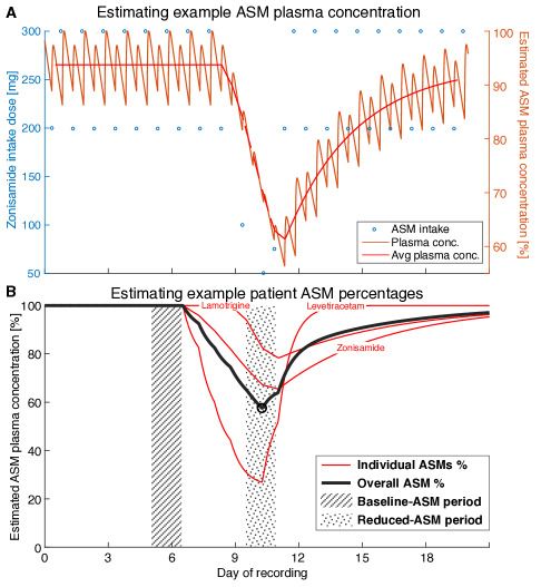
Figure 1: Estimating ASM plasma concentration and identifying baseline- and reduced-ASM periods. A Example medication (Zonisamide) in an example subject, with intake dosage (blue circles) over time, and the estimated ASM plasma concentration percentage based on the pharmaco-kinetic model (orange line). 24 h rolling mean of the plasma concentration over time is also shown in red. B Same example subject as A, with three different 24 h rolling mean ASM percentages (red lines) and the average thereof (thick black line) as an estimate of overall ASM tapering. The baseline-ASM period (hatched area) is identified as the 24 h before the first drop in the black line and the reduced-ASM period (dotted area) is the 24 h around the lowest point of the black line (marked by a black circle).

2.4 EEG data and processing

Our icEEG processing followed the same pipeline as our previous work (Wang et al., 2023, Panagiotopoulou et al., 2023), and a summary is replicated below.

Firstly, we divided each subject’s icEEG data into 30 s non-overlapping, consecutive time segments. All channels in each time segment were re-referenced to a common average reference. In each time segment, we excluded any noisy channels (with outlier amplitude ranges) from the computed common average. Missing data were not tolerated in any time segment and denoted as missing for the downstream analyses. Seizures and other provocation procedures - such as cortical stimulation and sleep deprivation/alteration - were removed from our analysis. All 30 s segments containing seizure data, or within 5 minutes of provocation periods, were removed and considered missing.

To remove power line noise, each time segment was notch filtered at $50$ Hz. Segments were band-pass filtered from $0.5-80$ Hz using a $4^{th}$ order zero-phase Butterworth filter (second order forward and backward filter applied) and further down-sampled to $200$ Hz. We then calculated the icEEG band power in the delta frequency band (1-4 Hz) for all channels and each 30 s time segment using Welch’s method with 3 s non-overlapping windows. In detail, for each channel in every 2 s window, we calculated the power spectral density and used Simpson’s rule to obtain the band power values, which were then averaged over all time windows within a 30 s segment to get the final band power values. We $log_{10}$-transformed the band power values, thus obtaining, for each subject, one matrix of log($\delta$ band power) at the ROI level. The size of each subject’s matrix was number of ROIs by number of 30 s segments.

Finally, from this matrix we retained data for the two time periods of interest: 24 h baseline-ASM and 24 h reduced-ASM.

2.5 Accounting for time-of-day effects

The time-of-day for the 24 h baseline-ASM period may not be aligned with the 24 h reduced-ASM period. For example, the first hour of baseline-ASM may fall on 14:00, whereas the first hour of reduced-ASM might be 17:00. As icEEG band power, especially $\delta$, is known to fluctuate strongly on a circadian timescale (Panagiotopoulou et al., 2022, 2023), we devised a method to account for the effect of the time-of-day.

First, band power for each ROI was averaged for each hour of the day. For example, all data collected between 04:00 to 04:59 was averaged to a single value per ROI. If the hour segment had more than $75\%$ of the data missing, the entire hour is considered as missing. Next, data were rearranged to match the time-of-day series from 00:00 to 23:00. For example, if the initial interval corresponds to 04:00, the final 4 hours after midnight were moved to the beginning, resulting in 24 hourly averages beginning at 00:00-00:59 and ending at 23:00-23:59. Matrices in Figure 2A&B demonstrate the hourly average and alignment procedure for an example subject’s baseline-ASM and reduced-ASM periods respectively, where each column corresponds to an hour, and each row an ROI.

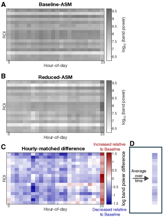
Figure 2: Log $\delta$ band power difference estimation process for a single subject accounting for time-of-day effects. A Baseline-ASM data matrix and B Reduced-ASM data matrix, where each row represents a ROI, each column an hour of the day and the grey-scale the log $\delta$ band power. C Colour-coded difference matrix between reduced-ASM relative to baseline-ASM, where red represent an increased relative to band power, blue a decrease and white no change. D Average of C over time (one value per ROI) following the same colour-code.

The difference between the two periods was obtained by subtracting the baseline-ASM matrix from the reduced-ASM matrix to produce Figure 2C. This resultant difference matrix captures the effect of ASM tapering on an hourly basis, accounting for the time-of-day effect. Finally, to achieve an average estimate of the effect of ASM tapering, we average the difference matrix over time (Figure 2D), thus obtaining a vector of tapering effects for each region recorded.

2.6 Statistical analyses

We report p-values as an additional reference to the tapering effect size, but we do not threshold the p-values to dichotomise our data further or make subsequent analysis decisions.

To determine if there were any differences between the baseline-ASM and reduced-ASM periods across subjects, we obtained the time-averaged band power difference between them in each region and each subject. We tested if the distribution of band power differences between baseline-ASM and reduced-ASM is different to 0 using non-parametric Wilcoxon signed rank tests. We subsequently correlated the magnitude of the ASM tapering with the band power change between baseline-ASM and reduced-ASM using Spearman’s rank correlation. To determine regional effects on the band power changes, we divided all ROIs into two categories: cortical and sub-cortical regions (in this case, Amygdala and Hippocampus); and we repeated the analysis for each category.

An additional, confirmatory analysis using hierarchical models accounting for subject-level differences in the location and number of regions recorded is presented in Supplementary S4. For simplicity, we only present the simpler, single-level model in the main text. These hierarchical models are used to confirm the relationships with ASM tapering magnitude, the regional difference between sub-cortical and cortical regions, and to investigate the effect of cortical lobes. Additionally, hierarchical models were used to analyse some confounding factors: differential effects of seizure onset zones, frequently-spiking regions, and later surgically removed regions; tapering of different ASM types; and the influence of recovery from anaesthesia post implantation.

Finally, we also disaggregate for the time-of-day effect. Instead of averaging over the 24 h period to study the band power change, we repeated our analysis for each hourly average (i.e. on the matrix of Figure 2C).

2.7 Code and Data

Anonymised EEG band power data and ASM intake schedule, along with analysis code will be available on Github: https://github.com/cnnp-lab/2024_ASM_EEG

3 Results

3.1 Subject and data characteristics

We included 22 individuals who underwent ASM tapering and had two 24 h icEEG data segments available for baseline-ASM and reduced-ASM states. The male:female distribution was 8:14, with an average age of 31.3(±8.6) years. In terms of epilepsy, individuals were diagnosed with temporal(16) and frontal(6) lobe epilepsy, affecting either left(10) or right(12) hemispheres.

We further summarised the ASM types used among the 22 individuals in Supplementary S1. The most frequently-used ASMs were Levetiracetam ($45\%$), Lamotrigine ($41\%$) and Clobazam ($36\%$). The average time between the start of medication tapering and reaching the minimum ASM level was approximately 2 days and 10 h (Supplementary S1).

In addition, we analysed 10 individuals with icEEG monitoring, but no ASM tapering in Supplementary S4.5 to support our main results.

3.2 icEEG band power decreases are correlated with medication tapering

We found an overall decrease in $\delta$ band power across all subjects between baseline-ASM and reduced-ASM states, after accounting for time-of-day effects. The distribution of $\delta$ band power changes over all regions and subjects (Figure 3A), and is on average decreasing (signed rank test effect size: -0.489, p$<$0.001). Averaging over all regions first in each subject yields similar results (signed rank test effect size: -0.626, p=0.003). As reported on Supplementary S3, a decreased band power was also found in other frequency bands. However, the lowest average value was seen in the $\delta$ band, and we therefore focus on this band for the main results.

Considering that each subject has been tapered off their ASMs to a different degree, we investigated if the $\delta$ band power decrease was tapering dose-dependent. Figure 3B shows the $\delta$ band power decrease against the relative percentage of ASM tapering for all subjects and ROIs. We observe a tendency of greater decrease in $\delta$ band power as ASMs are tapered to a lower level (Spearman’s rank correlation: 0.535, p<0.0001). Supplementary S4.1 additionally shows confirmatory results using a hierarchical model to account for regional and subject-level effects.

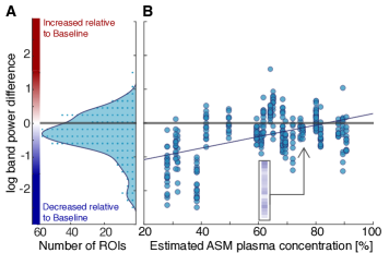
Figure 3: Tapering effects on log($\delta$ band power) for all subjects and ROIs. A Histogram across all ROIs and subjects of log($\delta$ band power) difference relative to baseline (each dot equates to 3 datapoints). B Scatter plot between log($\delta$ band power) difference relative to baseline (y-axis) and the recorded ASM percentage at the point of strongest tapering (black circle in Figure 1B) in each subject (x-axis). Data for all ROIs in a single subject line up on one value of ASM tapering percentage for that subject. For each subject, the underlying data is equivalent to Figure 2D.

We further investigated ASM-type-dependency by classifying medications based on their physiological target (Supplementary S4.3 for further details). Using a hierarchical model we observed that no ASM class had a distinctive effect on $\delta$ band power. We report all relevant statistics in Supplementary S4.3.

We also considered if any additional long-term effects might be present, such as the wearing-off of anaesthesia following surgery for implantation. We therefore investigated if the time between surgery and the baseline-ASM period impacted our results, and found no evidence of this (see Supplementary S4.4 for full stats tables).

Finally, to further test the robustness of the observed dose-dependent effect of $\delta$ band power decrease, we added the 10 subjects that were not ASM-tapered to our analysis as additional datapoints at ‘full-dose’. These additional subjects did not change the model coefficients substantially (and all p-values remained similar), further supporting the robustness of the model. Full details can be found in Supplementary S4.5.

3.3 Differential regional effects of ASM tapering

We disaggregated the previous analysis into cortical and sub-cortical (Amygdala and Hippocampus) regions, and found that the $\delta$ band power decrease was primarily seen in cortical brain regions (Figure 4).

In the sub-cortical regions, we found no evidence of delta band power decreases (signed rank test effect size: -0.076, p=0.628), whilst in the cortical regions the previously reported decrease remains (signed rank test effect size: -0.535, p$<$0.001). The relative percentage of ASM tapering influences both regions, although the effect was stronger in cortical regions (Spearman’s rank for cortical correlation: 0.566, p$<$0.001 and sub-cortical correlation: 0.362, p=0.021). Further analysis using a hierarchical model confirmed the dose-dependent effect on cortical regions but showed no evidence of dose-dependent effect for sub-cortical regions (see Supplementary S4.1). We used this same modelling approach to investigate whether specific cortical lobes are driving the observed effect, but found no evidence of this.

Finally, we tested if seizure onset regions showed a differential effect compared to other regions, factoring in the observed cortical and sub-cortical difference and subject-level effects, but we found no evidence of this (see Supplementary S4.2). Similarly, regions that were marked as frequently-spiking, and regions that were later removed by epilepsy surgery showed no differential effect either (Supplementary S4.2).

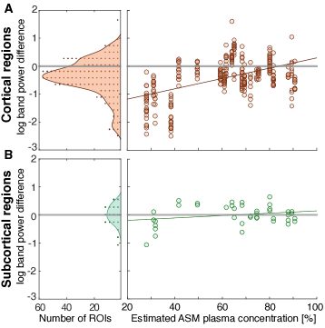
Figure 4: ASM tapering reduces $\delta$ band power in cortical but not sub-cortical regions. Plotting convention is the same as Figure 3. A The difference between the log($\delta$ band power) before and during tapering in cortical regions for each subject. B The difference between the log($\delta$ band power) before and during tapering in sub-cortical regions for each subject. In our data, only Amygdala and Hippocampus are recorded.

3.4 Circadian profile of ASM tapering effect

In all prior analysis, we analysed the average effect of ASM tapering over a 24 h period, after factoring out time-of-day effects by calculating band power differences on matched hours between baseline-ASM and reduced-ASM. In our final analysis, we disaggregated our results by the time-of-day, on an hourly basis. Figure 5A shows a stronger decrease of $\delta$ band power during daytime, particularly in cortical regions (Figure 5B).

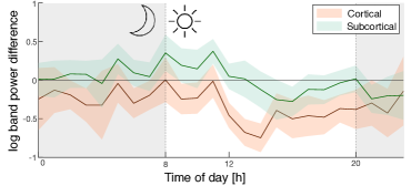
Figure 5: Log($\delta$ band power) difference relative to baseline-ASM resolved along the hours of the day. Solid lines represent the mean across ROIs and subjects, and shadows represent the $95\%$ confidence interval across subjects, for cortical (orange) and sub-cortical (green) regions.

4 Discussion

In this study, we confirmed previous observations that ASM tapering is associated with neurophysiological changes in icEEG (Duncan et al., 1989). More specifically, we saw a reduction in band power, particularly in the $\delta$ band, in all subjects and primarily cortical regions. Importantly, the observed reduction was linearly dependent on the strength of the tapering, further supporting a direct causal link.

A variety of ASM-mediated neurophysiological effects - including the effects of tapering and withdrawal - have been reported (Dini et al., 2023, Höller et al., 2017), and our study is most comparable in its retrospective design based on icEEG to that of Zaveri et al. (2010). We find it encouraging that we were able to directly reproduce their result of band power reduction, which was most strongly expressed in the $\delta$ band, followed by a weaker reduction in $\theta$ and $\alpha$ bands, with negligible effects in $\beta$ and $\gamma$ bands. We further replicated the “wide-spread” nature of this effect as reported by Zaveri et al. (2010). This independent replication in a completely separate cohort, in a different country, suggests that this is a reliable effect to leverage for future translational research.

We substantially expanded on previous studies by additionally presenting a dose-dependent effect, and differential effect in cortical regions and by considering time-of-day. We were able to show that the dose-dependent effect of $\delta$ band power decrease with tapering is essentially a cortical-only effect. The Amygdala and Hippocampal regions did not see a substantial or systematic change in band power with ASM tapering. This observation of a cortical vs. sub-cortical effect suggests that the observed band power change is not a purely technical consequence of e.g. drift in electrode properties (Ung et al., 2017, Campbell and Wu, 2018), which we further confirmed with a separate cohort that were not tapered in their ASMs (Suppl. S4.5).

Our sample size was too small to carry out a region-specific analysis, but our analysis did not show evidence of further spatial differentiation within the cortex. We also saw no differential effect in seizure onset, frequently-spiking, or later resected regions. This is in contrast to some previous studies that found a differential effect in other signal metrics in the SOZ (Sathyanarayana et al., 2024, Paulo et al., 2022). However, the effects reported in Sathyanarayana et al. (2024) were within higher frequency bands and used a different approach.

Studying the specific effects of ASM types was also not possible, as no subjects were on exactly the same combination of ASM types and steady-state dosages. The ASM classification aided, and allowed us to perform hierarchical modelling to observe possible changes. The fact that none of the defined classes had a significant effect can be explained by the heterogeneous effects of ASM types within the same class (Dini et al., 2023). However, there was a trend in multi-target ASMs, which could indicate a predominant effect of Sodium Valproate, which is known for having a strong effect on $\delta$ band power (Clemens et al., 2006).

Together, these observations may suggest that future work investigating the mechanisms of ASMs in epilepsy needs to account for the major structural and functional differences in the Amygdala and Hippocampus compared to the cortex, but specific epileptogenic alterations in the brain may be too heterogeneous to study in this context and much larger homogeneous samples are needed.

Our final key observation was that the tapering induced $\delta$ band power decrease was also dependent on the time-of-day, with the daytime hours showing the largest decrease. Unfortunately, the information about the sleep/wake status of each subject was not available retrospectively, hence we can only assume that the daytime hours primarily contain awake-states across the cohort (Roebber et al., 2022). With this assumption, our results could be interpreted as a $\delta$ band power decrease during wakefulness as opposed to sleep. Sleep and drowsiness have their own neurophysiological architecture and markers (Jin et al., 2020), and epileptic spikes occur more frequently in sleep. We therefore cautiously hypothesise that ASM tapering does not have a strong or consistent effect on band power composition, or spike properties during sleep. The latter hypothesis is additionally supported by our observation that frequently-spiking regions did not show evidence of a differential effect compared to other regions (Suppl. S4.2). Naturally, these hypotheses need to be differentiated and tested further in terms of ASM type, sleep architecture, and spike neurophysiology.

Despite clear advantages in our study, including dose-dependency analyses, regional differentiation, and accounting for time-of-day effects, our relatively small sample size limited our statistical power to discover potential effects in combinations of factors (such as type of epilepsy, or the combination of ASM types and brain regions). Furthermore, our ASM plasma levels were estimated based on pharmaco-kinetic assumptions, and not validated with actual plasma measurements. We also did not have information on the sleep/wake state of the subjects, limiting us to a time-of-day analysis only. Finally, our results should only be interpreted in the context of a temporary withdrawal (tapering) of ASM from steady-state levels in an adult, drug-refractory, and “difficult-to-treat” cohort; they may not be applicable in the context of adjusting medication dose for individuals starting on ASMs.

With this study, we hope to provide key insights toward the goal of biomarker discovery for temporary ASM withdrawal (Sathyanarayana et al., 2024). If validated in e.g. scalp EEG, or subcutaneous EEG, this approach enables a non/minimally-invasive real-time medication effect assessment, enabling medication reminder systems, integrating chronotherapy (Manganaro et al., 2017, Ramgopal et al., 2013), and closed-loop ASM delivery systems (Cook et al., 2020). Using an EEG marker has the clear advantage that we are measuring the medication effect in the central nervous system. ASMs are also used in other neurological and psychiatric conditions, making our findings relevant to application in, for example, anxiety disorders, migraine, neuropathic pain, and depression and mood disorders.

5 Acknowledgments and Funding

We thank members of the Computational Neurology, Neuroscience & Psychiatry Lab (www.cnnp-lab.com) for discussions on the analysis and manuscript; P.N.T. and Y.W. are both supported by UKRI Future Leaders Fellowships (MR/T04294X/1, MR/V026569/1). JSD, JdT are supported by the NIHR UCLH/UCL Biomedical Research Centre.

figuresection tablesection

Supplementary

S1 Subject and ASM details

N	22
Age (mean±SD)	31.1±8.6
Sex (M:F)	8:14
Epilepsy (Temporal:Frontal)	16:6
Side (Left:Right)	10:12
Num icEEG contacts (mean±SD)	71.1±27.0
Num ROIs (mean±SD)	16.3±5.6
Days of recording (mean±SD)	8.1±5.0
Num of regular ASM (mean±SD)	2.5±0.9
Num of tapered ASM (mean±SD)	2.3±0.9

Table 1: Summary of subject data used in the analysis.

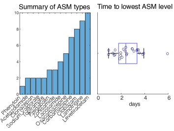
Figure S1: A Histogram of number of subjects receiving each ASM type. B Distribution of the time between the start of medication tapering and reaching the minimum ASM plasma levels ($avr=2.45days$).

S2 Plasma concentration modelling with first-order pharmaco-kinetics

As reported in the Methods, we used pharmaco-kinetic modelling to better represent the effects of ASMs on the electrophysiology. Here, Equation 1 is used to model the effect on plasma concentration of a single ASM intake with a first-order absorption and elimination. Considering all subjects included in this dataset, there are 13 different ASMs, listed in Figure S1A and Table 2. The parameters used in Equation 1 are exclusive for each ASM. All parameters but elimination (Ke) and absorption (Ka) constant have been obtained from DB , Patsalos (2022), Iapadre et al. (2018) considering the parameters of each medication from a single site. Ke and Ka had to be estimated from 2 other parameters: time to maximum concentration ($T_{max}$) and elimination half-life ($t_{1/2}$).

ASM	Tmax	t1/2	Ka	Ke	F	Vd	Tmax(Solver)
Levetiracetam	1.30	7.0	2.618	0.099	1.00	0.60	1.30
Lamotrigine	3.10	55.5	1.572	0.012	0.98	1.10	3.10
Clobazam	1.25	32.0	4.244	0.022	1.00	1.43	1.25
Carbamazapine	6.00	14.5	0.403	0.048	0.80	1.00	6.00
Oxacarbazepine	4.50	9.0	0.487	0.077	1.00	0.70	4.50
Zonisamide	4.00	63.0	1.180	0.011	0.95	1.45	4.00
Sodium Valproate	4.00	11.0	0.644	0.063	0.90	0.16	4.00
Pregabalin	1.50	6.3	2.065	0.110	0.90	0.50	1.50
Lacosamide	1.00	13.0	4.486	0.053	1.00	0.60	1.00
Topiramate	3.05	21.0	1.215	0.033	0.80	0.70	3.05
Clonazepan	2.50	60.0	2.091	0.012	0.90	3.00	2.50
Acetazolamide	3.00	12.5	1.029	0.055	0.90	0.30	3.00
Phenytoin	8.00	22.0	0.322	0.032	1.00	0.75	8.00

Table 2: Pharmaco-kinetic parameters for ASMs included in this study. F, bio-availability. Ka, absorption constant. Ke, elimination constant. t_1/2, elimination half-life. Vd, volume distribution. T_max, time to maximum plasma concentration. T_max(Solver), time to maximum plasma concentration estimated by Microsoft Excel Solver and Equation2

Ke estimation was calculated as: $ln(2)/t_{1/2}$. The estimation of Ka was obtained by resolving Equation 2. Given its complexity, an optimisation method was applied: Microsoft Excel Solver. Solver adjusts one or several cells to match a formula cell to a specific target. In our case, we have our formula of Equation 2 as well as the values of Ke and T_max obtained from the literature. For a specific ASM, we defined a new cell, T_max(Solver), as the result of implementing Equation 2 using cells for Ke and Ka. Then, Solver tool is configured to modify the value of Ka and match the value of T_max(Solver) with T_max. Once the process is finished, the new values of Ka and T_max(Solver) are automatically stored. This process is repeated individually for each ASMs.

$$T_{\text{max}}=\frac{ln(\frac{Ka}{Ke})}{Ka-Ke}$$ (2)

Equation 2: Pharmaco-kinetics equation to estimate time to maximum plasma concentration of a single dose oral intake with first order absorption and elimination. T_max, time to maximum plasma concentration. Ka, absorption constant. Ke, elimination constant.

The result from Equation 1 is the influence of a single ASM intake on plasma concentration. To model the continuous intakes and tapering for a specific subject, we combined several modelled influences, modifying the dose and the time of intake to match clinical reports. To complete the plasma concentration modelling, the steady-state concentration has to be modelled as well. The steady-state is reached after a prolonged and continuous ASM intake, and the required time changes between drugs. We approached this task by extending the intake schedule for a long period - 2 months before icEEG recordings started - following the regular treatment of each individual. Once modelled, the extra period is removed.

S3 ASM tapering effect on canonical frequency bands

In addition to the $\delta$ frequency band, we also explored the effect of ASM tapering on the other canonical frequency bands: Theta ($\theta$: 4-8 Hz), Alpha($\alpha$: 8-13 Hz), Beta ($\beta$: 13-30 Hz) and Gamma ($\gamma$: 30-47.5 Hz, 52.5-57.5 Hz, 62.5-77.5 Hz). Following the same analysis presented in the main text, we measured the change in log₁₀ power of each frequency band between the pre-tapered period and the tapered period. To better understand these changes, we also obtained the change in relative band power, as the contribution of each frequency band to the sum of the log₁₀ band power of each canonical frequency bands.

From the data presented in Figure S2 and Table 3, we can determine that the ASM tapering is generating an overall band power reduction with a spectral shift. Band power change is strongest for $\delta$ and gradually weakens as the frequency increases, showing no change for $\gamma$. Wilcoxon signed rank test confirms this behaviour - $\delta$ to $\beta$ negative size effects are observed with a strong significance. In contrast, changes in $\gamma$ show small size effects with no significance. In terms of relative band power, from $\delta$ to $\alpha$ a reduction is observed (only significant on $\delta$), while $\beta$ and $\gamma$ show a significant increase in relative band power. These two findings combined reveal that there is an overall reduction of band power on top of the spectral shift, where high frequency bands are less affected due to tapering than low frequency bands.

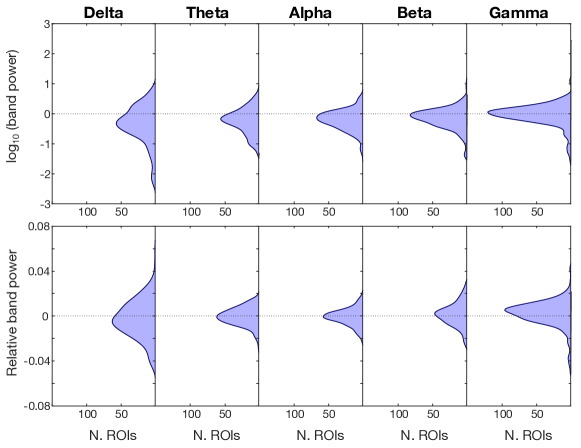
Figure S2: Distribution of $\delta$, $\theta$, $\alpha$, $\beta$ and $\gamma$ band power (Top Row) and relative band power (Bottom Row) changes due to tapering for all ROIs and subject

		$\delta$	$\theta$	$\alpha$	$\beta$	$\gamma$
log10 Band Power	Eff. Size	-0.489	-0.505	-0.558	-0.418	-0.037
	p-Value	$<$0.001	$<$0.001	$<$0.001	$<$0.001	0.484
Relative Band Power.	Eff. Size	-0.148	-0.029	-0.084	0.123	0.311
	p-Value	0.0047	0.582	0.120	0.019	$<$0.001

Table 3: Effect size and p-value of Wilcoxon signed rank test for band power (Top Row) and relative band power (Bottom Row) changes due to tapering on $\delta$, $\theta$, $\alpha$, $\beta$ and $\gamma$ frequency bands

S4 Hierarchical model predicting band power changes

We used hierarchical modelling throughout our study to assist us in confirming some of our findings while considering the influence of confounding factors. We built several hierarchical models as mixed-effect linear models with a common framework: $\delta$ log₁₀ band power changes in each ROI ($\triangle\delta$) are predicted, based on a random-effect for individual subjects (ID), and modifying the fixed-effects to test each case.

S4.1 Confirming effects of tapering strength and its regional differences

Adjusting for subject-effect using the mixed-effects model confirmed the effects of tapering strength and its regional differences. We fitted two mixed-effect linear models with fixed effects for: A) the relative percentage of the lowest ASM level reached during tapering (minASM):
$\triangle\delta$ $\sim$ 1 + minASM + (1$\mid$ID), Table 4 1^st panel;
B) the interaction between minASM and the classification of each ROI as cortical or sub-cortical (CORT):
$\triangle\delta$ $\sim$ 1 +minASM*CORT + (1$\mid$ID), Table 4 2^nd panel.

The fitted models confirm most of our findings with the Wilcoxon signed rank test and Spearman’s rank correlation, but refutes the dose-dependant effect observed on sub-cortical regions. As observed in Table4 2^nd panel, only the cortical region shows an overall decrease of $\delta$ band power and a dose-dependent effect on it.

Model	Fixed-Effect	Estimate	p-Value
minASM	minASM	1.377	0.008
minASM*CORT	Inter.(Sub-cortical)	-0.499	0.194
	minASM	0.709	0.219
	Cortical	-0.835	$<$0.001
	minASM:Cortical	0.755	0.012
minASM*Lobe	Inter.(Occipital)	-0.980	0.026
	Frontal	-0.688	0.039
	Cingulate	-0.165	0.692
	Temporal	-0.147	0.632
	Parietal	-0.729	0.015
	minASM	0.953	0.016
	minASM:Frontal	1.050	0.042
	minASM:Cingulate	0.372	0.558
	minASM:Temporal	0.201	0.668
	minASM:Parietal	0.984	0.034

Table 4: Table showing the coefficient estimates and p-values of the fixed-effect predictors for the following mixed-effect linear models from top to bottom: 1) $\triangle\delta$ $\sim$ 1 + minASM + (1$\mid$ID); 2) $\triangle\delta$ $\sim$ 1 +minASM*CORT + (1$\mid$ID); 3) $\triangle\delta$ $\sim$ 1 + minASM*Lobe + (1$\mid$ID). Predictors “CORT” and “Lobe” are categorical values, therefore intercept (Inter) represent the category on brackets.

We also explored further parcellation of cortical regions dividing it into lobes (Lobe): Frontal, Cingulates, Parietal, Temporal and Occipital:
$\triangle\delta$ $\sim$ 1 + minASM*Lobe + (1$\mid$ID), Table 4 3^rd panel.
The resulting model reveals that all cortical regions have similar decrease of $\delta$ band power and a dose-dependent behaviour.

S4.2 Seizure onset, frequently-spiking or later surgically resected regions do not have characteristic behaviour

In addition to regional differences the effects of ROIs being within the seizure onset zone (SOZ), later surgically resected areas (RSC), or frequently-spiking (SPK), have also been studied. We labelled each ROI as SOZ, RSC or SPK based on the number of channels within these categories applying thresholds of 1 channel for SOZ and 25% for RSC and SPK. We fit the independent mixed-effect models with a fixed effect for the interaction between each label and cortical parcellation ($\triangle\delta$ $\sim$ 1 + SOZ*CORT + (1$\mid$ID)), to determine if there are behavioural changes on SOZ, RSC or SPK areas. Table 5 shows that seizure onset zones, surgically resected areas and spiking regions show no distinctive behaviour compared to the rest of the tissue.

Model	Fixed-Effect	Estimate	p-Value
SOZ*CORT	Inter.(Sub-cortical $\&$ nSOZ)	-0.091	0.513
	SOZ	0.035	0.765
	Cortical	-0.330	$<$0.001
	SOZ:Cortical	0.046	0.721
RSC*CORT	Inter.(Sub-cortical $\&$ nRSC)	-0.022	0.878
	RSC	-0.073	0.524
	Cortical	-0.398	$<$0.001
	RSC:Cortical	0.107	0.397
SPK*CORT	Inter.(Sub-cortical $\&$ nSPK)	-0.082	0.670
	SPK	0.0141	0.934
	Cortical	-0.336	0.036
	SPK:Cortical	0.014	0.936

Table 5: Table showing the coefficient estimates and p-values of the fixed-effect predictors for the following mixed-effect linear models from top to bottom: 1) $\triangle\delta$ $\sim$ 1 + SOZ*CORT + (1$\mid$ID); 2) $\triangle\delta$ $\sim$ 1 + RSC*CORT + (1$\mid$ID); 3) $\triangle\delta$ $\sim$ 1 + SPK*CORT + (1$\mid$ID). Predictors “CORT”, “SOZ”, “SPK” and “RSC” are categorical variables, therefore intercept (Inter.) represent the combination of categories on brackets.

S4.3 Similar behaviour among ASM classes

As reported in the literature, different ASMs have specific effects on each of the canonical frequency bands. Our low sample size and the heterogeneity of ASM use during tapering makes studying individual medication effects unreliable. Therefore, we classified ASMs based on their primary physiological target. As an example, Clobazam and Clonazepam are classified as “GABA-ergic” (GB) due to mostly affecting gabba receptors, while Carbazapine and Oxarbazapine as “Sodium Channels” (SC). All ASM are classified into 5 groups: GABA-ergic (GB), Sodium Channel (SC), SV2A receptor (SV), Multi-targel (ML) and Other Targets (OT, including ASM classifications with low representations). As ASMs belonging to multiple classes can be tapered at the same time, each one is assigned a binary variable and the intercept is removed as all subjects that had at least 1 ASM tapered - a simplification will be used going forward where $ASM_{c}$ = SC+ML+GB+SV+OT-1. The fitted model captures the effect of each ASM class and the reduction of ASM plasma concentration level reached with them (minASM). We only considered cortical ROIs for this analysis, as sub-cortical regions show no significant changes due to tapering. The resulting model ($\triangle\delta$ $\sim$ 1 + $ASM_{c}$*minASM + (1$\mid$ID), Table 6) indicates that subjects tapered with Multi-Target ASM have stronger overall $\delta$ band power reduction but no dose-dependency.

Model	Fixed-Effect	Estimate	p-Value
minASM*ASMc	minASM	-0.481	0.463
	SC(t)	-0.217	0.831
	ML(t)	-2.128	0.087
	GB(t)	-0.324	0.727
	SV(t)	-1.341	0.183
	OT(t)	1.640	0.451
	minASM:SC(t)	0.429	0.767
	minASM:ML(t)	3.394	0.09
	minASM:GB(t)	0.289	0.846
	minASM:SV(t)	2.036	0.197
	minASM:OT(t)	-2.260	0.493

Table 6: Table showing the coefficient and p-values of the fixed-effect predictors for mixed-effect linear model $\triangle\delta$ $\sim$ 1 + $ASM_{c}$*minASM + (1$\mid$ID).

S4.4 Recovery time from surgery does not affect band power changes

All subjects included in our study underwent surgery for icEEG electrode implantation. Several factors related to the surgery and its recovery have the potential of affect the icEEG recordings: recovery from anaesthesia, inflammatory processes, stress of a prolonged hospitalisation and others. Therefore, we built a hierarchical model to determine if the duration of time between surgery to tapering has an effect on the observed band power changes. This time gap (SGRt) is defined as the time between the day of the surgery and the end of baseline-ASM period - the first instance when tapering effects are observed. The selected definition for SGRt prevents its interaction with the minimum ASM level reached during tapering (minASM) when the hierarchical model is fitted.

The applied hierarchical model captures the effects of these two parameters and regional differences between cortical and sub-cortical regions ($\triangle\delta$ $\sim$ 1 + (minASM+SRGt)*CORT + (1$\mid$ID), Table 7) and reveals that a longer time since surgery does not have a significant effect on $\delta$ band power changes.

Model	Fixed-Effect	Estimate	p-Value
(minASM+SRGt)*CORT	Inter.(Sub-cortical)	-0.476	0.250
	minASM	0.569	0.322
	SRGt	0.012	0.837
	Cortical	-1.054	$<$0.001
	Cortical:minASM	0.637	0.040
	Cortical:SRGt	0.056	0.12

Table 7: Table showing the coefficient estimates and p-values of the fixed-effect predictors for mixed-effect linear $\triangle\delta$ $\sim$ 1 + (minASM+SRGt)*CORT + (1$\mid$ID) applied on tapered individuals. Predictors “CORT” is a categorical variable, therefore intercept (Inter.) represent the category in brackets.

S4.5 Not ASM tapered cohort

In addition to tapered subjects, we have also investigated a sample of icEEG monitoring subjects that did not undergo ASM tapering. These subjects were experiencing seizures regularly even on full ASM dose, making tapering unnecessary. This likely reflects either a difference in disease aetiology or in other factors such as the stress of surgery that may have lowered seizure threshold. This, combined with differences in proximity to surgery, and icEEG recording duration, makes direct comparisons between tapered and not tapered subjects difficult. However, here we have attempted to make accommodations, allowing us to include these subjects in a limited analysis.

To reflect that these individuals did not go through ASM tapering and were constantly at ‘full-dose’, the minimum ASM plasma concentration level was set to 1. To obtain the 24 h time windows of baseline-ASM and reduced-ASM, we attempted to replicate the distribution of the time distances between surgery, start of tapering and minimum ASM levels on tapered subject. First, we obtained these time distances (surgery to start of tapering, and start of tapering to minimum ASM) for all tapered subjects, and extracted the mean, standard deviation, maximum and minimum values. These values are used to generate random time distance values that fit on the distribution defined by the mean and standard deviation, and keeping them within the maximum and minimum values. However, because the overall length of the recordings is shorter for non-tapered subjects, the time between surgery, baseline-ASM, and reduced-ASM is shorter than for the tapered subjects.

We added 10 not tapered subjects to our previous 22 tapered subjects and reproduced the hierarchical model presented in Suppl. S4.4. The resulting model (Table 8) showed no substantial change compared to the model fitted with only tapered subjects (Table 7). The similarity between models consolidates our findings, showing a consistent dose-effect while including subject on ‘full-dose’.

Giving the similarity between models, the complications introduced to the methodology by shorter recordings, and a likely difference in severity of the disease, we did not investigate the non-tapered subjects further.

Model	Fixed-Effect	Estimate	P-Value
(minASM+SRGt)*CORT	Inter.(Sub-cortical)	-0.082	0.863
	minASM	-0.712	0.143
	SRGt	0.070	0.220
	Cortical	-1.032	$<$0.001
	Cortical:minASM	0.542	0.072
	Cortical:SRGt	0.062	0.111

Table 8: Table showing the coefficient estimates and p-values of the fixed-effect predictors for mixed-effect linear model $\triangle\delta$ $\sim$ 1 + (minASM+SRGt)*CORT + (1$\mid$ID) applied on tapered and non tapered individuals. Predictors “CORT” is a categorical variable, therefore intercept (Inter.) represent the category on brackets.

References

- (1) Drug bank online. https://go.drugbank.com.
- (2) The national epilepsy and neurology database. https://www.hra.nhs.uk/planning-and-improving-research/application-summaries/research-summaries/national-epilepsy-neurology-database/. Accessed: 2024-02-07.
- Campbell and Wu (2018) Andrew Campbell and Chengyuan Wu. Chronically implanted intracranial electrodes: Tissue reaction and electrical changes. Micromachines (Basel), 9, 8 2018. doi: 10.3390/mi9090430. URL https://pubmed.ncbi.nlm.nih.gov/30424363/.
- Clemens et al. (2006) Béla Clemens, Andrea Ménes, Pálma Piros, Mónika Bessenyei, Anna Altmann, Judit Jerney, Katalin Kollár, Beáta Rosdy, Margit Rózsavölgyi, Katalin Steinecker, and Katalin Hollódy. Quantitative eeg effects of carbamazepine, oxcarbazepine, valproate, lamotrigine, and possible clinical relevance of the findings. Epilepsy Research, 70:190–199, 8 2006. doi: 10.1016/j.eplepsyres.2006.05.003. URL https://www.sciencedirect.com/science/article/pii/S0920121106001446?ref=pdf_download&fr=RR-2&rr=86b062d42b136a3d.
- Consales et al. (2021) Alessandro Consales, Sara Casciato, Sofia Asioli, Carmen Barba, Massimo Caulo, Gabriella Colicchio, Massimo Cossu, Luca de Palma, Alessandra Morano, Giampaolo Vatti, Flavio Villani, Nelia Zamponi, Laura Tassi, Giancarlo Di Gennaro, and Carlo Efisio Marras. The surgical treatment of epilepsy. Neurological Sciences, 42:2249–2260, 6 2021. ISSN 15903478. doi: 10.1007/S10072-021-05198-Y/METRICS. URL https://link.springer.com/article/10.1007/s10072-021-05198-y.
- Cook et al. (2020) Mark Cook, Michael Murphy, Kristian Bulluss, Wendyl D’Souza, Chris Plummer, Emma Priest, Catherine Williams, Ashwini Sharan, Robert Fisher, Sharon Pincus, Eric Distad, Tom Anchordoquy, and Dan Abrams. Anti-seizure therapy with a long-term, implanted intra-cerebroventricular delivery system for drug-resistant epilepsy: A first-in-man study. EClinicalMedicine, 3, 5 2020. doi: 10.1016/j.eclinm.2020.100326.
- Dini et al. (2023) Gianluca Dini, Giovanni Battista Dell’Isola, Elisabetta Mencaronia, Pietro Ferrar, Giuseppe Di Cara, Pasquale Striano, and Alberto Verrotti. The impact of anti-seizure medications on electroencephalogram (eeg) results. Expert Review of Neurotherapeutics, 23:559–565, 5 2023. doi: 10.1080/14737175.2023.2214315.
- Duncan et al. (1989) J S Duncan, S J Smith, A Forster, S D Shorvon, and M R Trimble. Effects of the removal of phenytoin, carbamazepine, and valproate on the electroencephalogram. Epilepsia, 5, 9 1989. doi: 10.1111/j.1528-1157.1989.tb05477.x.
- Dwivedi et al. (2017) Rekha Dwivedi, Prabhakar Tiwari, Monika Pahuja, Rima Dada, and Manjari Tripathi. Anti-seizure medications and quality of life in person with epilepsy. Heliyon, page e11073, 2017. doi: 10.1016/j.heliyon.2022.e11073. URL https://doi.org/10.1016/j.heliyon.2022.e11073.
- Fischl (2012) Bruce Fischl. FreeSurfer. NeuroImage, 62(2):774–781, August 2012. ISSN 10538119. doi: 10.1016/j.neuroimage.2012.01.021. URL https://linkinghub.elsevier.com/retrieve/pii/S1053811912000389.
- Ghosn et al. (2023) Nina J Ghosn, Kevin Xie, Akash R Pattnaik, James J Gugger, Colin A Ellis, Elizabeth Sweeney, Emily Fox, John M Bernabei, Jenaye Johnson, Jacqueline Boccanfuso, Brian Litt, and Erin C Conrad. A pharmacokinetic model of antiseizure medication load to guide care in the epilepsy monitoring unit. Epilepsia, 64:1236–1247, 5 2023. doi: 10.1111/epi.17558. URL https://pubmed.ncbi.nlm.nih.gov/36815252/.
- Hagmann et al. (2008) Patric Hagmann, Leila Cammoun, Xavier Gigandet, Reto Meuli, Christopher J Honey, Van J Wedeen, and Olaf Sporns. Mapping the Structural Core of Human Cerebral Cortex. PLoS Biology, 6(7):e159, July 2008. ISSN 1545-7885. doi: 10.1371/journal.pbio.0060159. URL https://dx.plos.org/10.1371/journal.pbio.0060159.
- Höller et al. (2017) Yvonne Höller, Christoph Helmstaedter, and Klaus Lehnertz. Quantitative pharmaco-electroencephalography in antiepileptic drug research. CNS Drugs, 32:839–848, 8 2017. doi: 0.1007/s40263-018-0557-x.
- Iapadre et al. (2018) Giulia Iapadre, Ganna Balagura, Luca Zagaroli, Pasquale Striano, and Alberto Verrotti. Pharmacokinetics and drug interaction of antiepileptic drugs in children and adolescents. Pediatr Drugs, page 429–453, 2018. doi: 10.1007/s40272-018-0302-4.
- Jin et al. (2020) Bo Jin, Thandar Aung, Yu Geng, and Shuang Wang. Epilepsy and its interaction with sleep and circadian rhythm. Frontiers in Neurology, 11:516572, 5 2020. ISSN 16642295. doi: 10.3389/FNEUR.2020.00327.
- Kanner and Bicchi (2022) Andres M Kanner and Manuel Melo Bicchi. Antiseizure medications for adults with epilepsy: A review. JAMA, 327:1269–1281, 4 2022. ISSN 1538-3598. doi: 10.1001/jama.2022.3880. URL http://www.ncbi.nlm.nih.gov/pubmed/35380580.
- Manganaro et al. (2017) Sheryl Manganaro, Tobias Loddenkemper, and Alexander Rotenberg. The need for antiepileptic drug chronotherapy to treat selected childhood epilepsy syndromes and avert the harmful consequences of drug resistance. Journal of Central Nervous System Disease, 9, 2017. doi: 10.1177/1179573516685. URL https://journals.sagepub.com/doi/full/10.1177/1179573516685883.
- Panagiotopoulou et al. (2022) Mariella Panagiotopoulou, Christoforos A. Papasavvas, Gabrielle M. Schroeder, Rhys H. Thomas, Peter N. Taylor, and Yujiang Wang. Fluctuations in eeg band power at subject-specific timescales over minutes to days explain changes in seizure evolutions. Human Brain Mapping, 43:2460–2477, 6 2022. doi: 10.1002/hbm.25796. URL https://onlinelibrary.wiley.com/doi/full/10.1002/hbm.25796.
- Panagiotopoulou et al. (2023) Mariella Panagiotopoulou, Christopher Thornton, Fahmida A Chowdhury, Beate Diehl, John S Duncan, Sarah J Gascoigne, Andrew W McEvoy, Anna Miserocchi, Billy C Smith, Jane de Tisi, Peter N Taylor, and Yujiang Wang. Diminished circadian and ultradian rhythms in pathological brain tissue in human in vivo. arXiv preprint arXiv:2309.07271, 9 2023.
- Patsalos (2022) Philip N. Patsalos. Antiseizure Medication Interactions - A Clinical Guide. Springer, 2022.
- Paulo et al. (2022) Danika L. Paulo, Kristin E. Wills, Graham W. Johnson, Hernan F.J. Gonzalez, John D. Rolston, Robert P. Naftel, Shilpa B. Reddy, Victoria L. Morgan, Hakmook Kang, Shawniqua Williams Roberson, Saramati Narasimhan, and Dario J. Englot. Seeg functional connectivity measures to identify epileptogenic zones. Neurology, 20:e2060–e2072, 5 2022. doi: 10.1212/WNL.0000000000200386. URL https://www.neurology.org/doi/10.1212/WNL.0000000000200386.
- Ramgopal et al. (2013) Sriram Ramgopal, Sigride Thome-Souza, and Tobias Loddenkemper. Chronopharmacology of anti-convulsive therapy. Curr Neurol Neurosci Rep, 13, 4 2013. doi: 10.1007/s11910-013-0339-2.
- Roebber et al. (2022) Jennifer K. Roebber, Penelope A. Lewis, Vincenzo Crunelli, Miguel Navarrete, and Khalid Hamandi. Effects of anti-seizure medication on sleep spindles and slowwaves in drug-resistant epilepsy. Brain Sci., 10:1288, 9 2022. doi: 10.3390/brainsci12101288.
- Sarangi et al. (2022) Sudhir C. Sarangi, Sachin Kumar, Manjari Tripathi, Thomas Kaleekal, Surender Singh, and Yogendra K. Gupta. Antiepileptic-drug tapering and seizure recurrence: Correlation with serum drug levels and biomarkers in persons with epilepsy. Indian Journal of Pharmacology, 54:24–32, 2 2022. doi: 10.4103/ijp.ijp˙253˙21. URL https://www.ncbi.nlm.nih.gov/pmc/articles/PMC9012412/.
- Sathyanarayana et al. (2024) Aarti Sathyanarayana, Rima El Atrache, Michele Jackson, Sarah Cantley, Latania Reece, Claire Ufongene, Tobias Loddenkemper, Kenneth D Mandl, and William J Bosl. Measuring real-time medication effects from electroencephalography. Journal of clinical neurophysiology : official publication of the American Electroencephalographic Society, 41:72–82, 1 2024. ISSN 1537-1603. doi: 10.1097/WNP.0000000000000946. URL http://www.ncbi.nlm.nih.gov/pubmed/35583401http://www.pubmedcentral.nih.gov/articlerender.fcgi?artid=PMC9669285.
- Ung et al. (2017) Hoameng Ung, Steven N. Baldassano, Hank Bink, Abba M Krieger, Shawniqua Williams, Flavia Vitale, Chengyuan Wu, Dean Freestone, Ewan Nurse, Kent Leyde, Kathryn A Davis, Mark Cook, and Brian Litt. Intracranial eeg fluctuates over months after implanting electrodes in human brain. J Neural Eng, 14, 9 2017. doi: 10.1088/1741-2552/aa7f40. URL https://pubmed.ncbi.nlm.nih.gov/28862995/.
- Wang et al. (2023) Yujiang Wang, Gabrielle M Schroeder, Jonathan J Horsley, Mariella Panagiotopoulou, Fahmida A Chowdhury, Beate Diehl, John S Duncan, Andrew W McEvoy, Anna Miserocchi, Jane de Tisi, et al. Temporal stability of intracranial eeg abnormality maps for localizing epileptogenic tissue. Epilepsia, 2023.
- Zaveri et al. (2010) Hitten P Zaveri, Steven M Pincus, Irina I Goncharova, Edward J Novotny, Robert B Duckrow, Dennis D Spencer, Hal Blumenfeld, and Susan S Spencer. Background intracranial eeg spectral changes with anti-epileptic drug taper. Clinical Neurophysiology, 121:311–7, 3 2010. doi: 10.1016/j.clinph.2009.11.081. URL https://pubmed.ncbi.nlm.nih.gov/20075002/.