High-frequency tails in spectral densities

Abstract

Recent developments in numerically exact quantum dynamics methods have brought the dream of calculating the dynamics of chemically complex open systems closer to reality. Path-integral-based methods, hierarchical equations of motion (HEOM) and quantum analog simulators all require the spectral density of the environment to describe its effect on the system. Here we find that the rate of slow population relaxation is sensitive to the precise functional form used to describe the spectral density peaks. This finding highlights yet another challenge to obtaining accurate spectral densities. We give a simple recipe to adjust the results of quantum simulation for this difference assuming both the simulator and the target spectral densities are known.

I Introduction

Accurate calculations of quantum dynamics of open quantum systems with chemically complex environments would advance our understanding of many problems of interest in chemistry, biology, and quantum information science. Tuning of the coherence times of molecular qubits,[1] learning from efficient energy transfer in photosynthesis,[2] and in silico design of molecular engines[3] - these are just select examples of the many new possibilities that would open up. Due to the inherent complexity of the open quantum dynamics, there isn’t a single universal approach to solve it. Instead, a great variety of methods has been developed, each of them with a different regime of applicability.

The main challenge in open quantum dynamics is to accurately describe the effect of a large environment on a small system of interest. The unitary dynamics of system plus environment are intractable owing to the large (possibly macroscopic) environment. Various approximate methods have been developed, that utilize convenient but often severe approximations: Markovian, secular, finite order perturbation theory, semiclassical, etc. These methods are much less demanding in terms of computational cost, but the validity of various approximations needs to be verified. We do not consider our findings in the context of these approximate methods. Historically, two main strategies to make the problem tractable without introduction of uncontrolled approximations emerged; we will refer to these two strategies as "unitary" and "reduced" for brevity. In the unitary approach, finite number of degrees of freedom of the environment are included and the total dynamics (of both system and truncated environment) is unitary. Multiconfigurational time-dependent Hartree (MCTDH),[4, 5] and its multilayer extension,[6] the density matrix renormalization group (DMRG),[7] the time-evolving density matrix using the orthogonal polynomials algorithm (TEDOPA),[8] the time-dependent Davydov ansatz,[9] and the effective-mode (EM) approach[10] all utilize this strategy. Only finite number of environment modes can be included, meaning that the overall dynamics is reversible. Thus, the system cannot reach thermal state even in principle and instead will experience recurrences in long-time dynamics. On the other hand, these methods are applicable to "tough" cases, such as anharmonic environment modes,[11] failure of the Born-Oppenheimer approximation,[12] or strong,[13] possibly nonlinear[5] coupling to the environment.

Hierarchical equations of motion (HEOM)[14] and its variants,[15, 16, 17] as well as real-time path integral (PI) methods[18, 19, 20, 21, 22, 23, 24] utilize the reduced strategy to make open quantum dynamics numerically tractable. "Reduced" here refers to the fact that only system dynamics is followed explicitly; the effect of the environment is captured implicitly by introducing a bath of large (possibly uncountably infinite) number of harmonic degrees of freedom, each bilinearly coupled to the system. The effect of this harmonic bath on the system dynamics on one hand can be captured exactly within an effective description,[25, 26] and on the other hand it can mimic[27, 28] the effect of a complex environment through Gaussian response. For example, recently, the relaxation in bacterial light harvesting chromophore has been simulated[29] using the small matrix decomposition of the path integral algorithm.[21] Similarly, HEOM was used to model the FMO complex.[30] While extensions to nonlinear system-bath couplings[31, 32] as well as approaches that utilize (anharmonic) spin baths[33, 34] have been developed, we will only consider the simplest case of linear coupling to harmonic bath, as this is the setting used in the vast majority of numerically exact calculations to date.

Recent advances on the intersection between quantum information science and theoretical chemistry opened up a radically new set of approaches to obtain accurate open quantum dynamics – using digital quantum computation[35, 36] or analog quantum simulation.[37, 38] The former has many of the strengths and weaknesses of the unitary methods, since quantum computers are naturally suited to describe unitary quantum dynamics. In contrast, quantum analog simulators can be used to realize open system dynamics with macroscopically large environments,[38] which groups them together with the reduced methods.

Both PI and HEOM methods are numerically exact, meaning the dynamics of the system can be described as accurately as needed by tightening convergence parameters appropriately. Assuming the dynamics is converged, the model we formulate to describe a process is the only remaining source of discrepancies between a numerically exact simulation and physical reality. In this paper we analyze the importance of faithful representation of a structured bath, illustrating our findings using the HEOM simulations.[17] However, we emphasize that our findings extend to any reduced approach (all HEOM variants, all real time PI methods, and quantum analog simulators with continuous baths).

The properties of any harmonic bath bilinearly coupled to the system are fully captured[25] by the bath spectral density (SD) defined in the frequency domain as

$$J(\omega)=\sum_{j}\hbar|g_{j}|^{2}\left(\delta(\omega-\omega_{j})-\delta(\omega+\omega_{j})\right)$$ (1)

with each bath mode $\omega_{j}$ characterized by the system-bath coupling constant $g_{j}$ and $\hbar$ denoting the reduced Planck’s constant. Note that there are alternative definitions of the spectral density in the literature with different prefactors[26] or different powers of frequency, for example Ref. [40] defines spectral density as $j(\omega)=J(\omega)/\omega^{2}$, which is more convenient for the interpretation of the optical properties.[41]

The spectral density enters the equations of motion of the open quantum system via the bath correlation function (BCF) also known as bath response function,[25]

$$C(t)=\int_{-\infty}^{\infty}d\omega J(\omega)f_{{BE}}(\beta\omega)e^{-i\omega t},$$ (2)

where as usual $\beta=(k_{B}T)$ is the inverse temperature multiplied by the Boltzmann constant, and $f_{BE}$ denotes the Bose-Einstein distribution $f_{BE}(x)=(1-e^{-x})^{-1}$.

Obtaining an accurate SD for a system interacting with a structured environment is highly nontrivial. Molecular dynamics (MD) or the hybrid quantum mechanics/molecular mechanics (QM/MM) methods can be used to calculate classical (i.e., real only) BCF and the SD can be constructed from it. [42, 43, 44] Experimental data can also inform construction of the SDfor a pure dephasing process. For instance, fluorescence line narrowing spectra[45, 46] or resonance Raman scattering spectra.[47] However, both experimental and theoretical approaches yield limited accuracy, such that the precise functional form of the SD that determines its decay rate at high frequency cannot be determined at present. Moreover, most implementations of HEOM variants require that the BCF is written as a finite sum of exponentials,[17, 15, 48, 16, 49]

$$C(t)\approx\sum_{j}c_{j}e^{i\Omega_{j}t},$$ (3)

with complex prefactors $c_{j}$ and complex $\Omega_{j}=\omega_{j}+i\gamma_{j}$, whose real and imaginary parts are related to the central frequency and broadening of the peak in spectral density. We note that the decompositions using other types of functions are possible within HEOM as well, for example as a sum of Bessel functions of first kind.[50] We will only consider exponential BCFs here.

Therefore, the choice of the functional form of SD in open dynamics simulations is frequently motivated by either the experimental constraints (for instance, when using RLC (resistor-inductor-capacitor) circuits to mimic bath degrees of freedom in quantum analog simulators)[38] or by the numerical efficiency considerations (as in HEOM variants where the Drude-Lorenz form is particularly efficient),[51, 41] or by the exact results in limiting cases (for example underdamped Brownian peaks which describe one vibrational mode coupled to the system as well as to a secondary harmonic bath).[52, 51, 41] Additionally, other numerically exact methods like quantum-classical path integral[22, 23] require the discretization of the bath, which necessarily implies a high-frequency cutoff and can obscure the functional form of the peak

In what follows, we will analyze the effect of using different functional forms to describe the features (i.e., peaks) of a given SD. The condition of Eq. (3) requires that each peak of the spectral density is represented with a fit function that has a small (but nonzero) number of first order (i.e., simple) poles in the lower half of the complex plane (see section II.2). We will also limit ourselves to only considering odd functions of frequency, such that the resulting spectral density is odd by construction, as required by Eq. (1). While these conditions might seem restrictive at first sight, we note that two of the most commonly used functional forms to model the spectral density (Drude-Lorenz and underdamped Brownian oscillators) satisfy them.[41, 51]

There are several excellent and comprehensive analyses of the impact of low-frequency end of the spectrum (i.e., $\lim_{\omega\rightarrow 0^{+}}J(\omega)\propto\omega^{s}$) on the dynamics of spin-boson and displaced oscillator models,[26] where $s=1$ (ohmic), $s<1$ (subohmic), and $s>1$ (superohmic) cases exhibit qualitatively distinct dynamics. By contrast, we have not found studies that analyze in detail the high-frequency end of the spectrum, which is the focus of this work.

The paper is organized as follows. We begin section II with a brief reminder of open quantum dynamics, then in section II.1 we describe the HEOM approach that allowed us to include chemically complex spectral density at tractable cost; we discuss representations of the spectral density peaks in section II.2. Finally, we detail the model system parameters in section II.3. We analyze the impact of the SD tails on the dephasing (section III.1) and population relaxation (section III.2) of a realistic system (electronic excitation of thymine-like molecule in water) and wrap up in section III.3 with the way to connect simulations with different SD basis functions valid in the limit where dephasing and population relaxation are decoupled by separation of timescales.

II Methods

We consider a quantum system coupled to harmonic bath and described by the total Hamiltonian split into the system $H_{s}$, bath $H_{b}$ and the system-bath interaction $H_{sb}=S\otimes B$ parts,

$$\hat{H}=\hat{H}_{s}+\hat{H}_{b}+\hat{S}\otimes\hat{B}=\frac{\hbar\Omega}{2}\hat{\sigma}_{z}+\sum_{j}\hbar\omega_{j}\left(\hat{a}_{j}^{\dagger}\hat{a}_{j}+\frac{1}{2}\right)+(\alpha_{z}\hat{\sigma}_{z}+\alpha_{x}\hat{\sigma}_{x})\otimes\sum_{j}\left(g_{j}\hat{a}^{\dagger}_{j}+g_{j}^{*}\hat{a}_{j}\right),$$ (4)

where $\hat{\sigma}_{z}=\ket{1}\bra{1}-\ket{0}\bra{0}$ and $\hat{\sigma}_{x}=\ket{0}\bra{1}+\ket{1}\bra{0}$ are the usual Pauli matrices with $\ket{0}$ and $\ket{1}$ denoting the ground and excited electronic state in the bra-ket notation. The system is characterized by the transition frequency between the ground and excited electronic states $\Omega$. The bath is assumed to be a collection of harmonic oscillatros with frequency $\omega_{j}$, so that $\hat{a}^{\dagger}_{j}$ and $\hat{a}_{j}$ are the usual bosonic creation and annihilation operators. Note that the dagger symbol is used throughout to denote the adjoint of an operator. Finally, the system-bath interaction term couples the collective bath coordinate (displacement-like bath operator) to the nondiagonal system operator weighted by $\alpha_{x}$ and $\alpha_{z}$, $\alpha_{z}^{2}+\alpha_{x}^{2}=\frac{1}{4}$. In Eq. (4) we consider the two-level system for simplicity, but the multi-state generalization is straightforward and the conclusions of our analysis carry over. Note that the assumption of harmonic bath does not restrict our considerations to the chemical environments that are harmonic, since the effects of an arbitrary anharmonic environment can be taken into account within Eq. (4) by using an appropriate spectral density, provided the interaction is described well without going beyond second order in perturbation theory,[26] which is expected for the macroscopically large environment in the thermodynamic limit, where interaction is distributed over many degrees of freedom.[27]

II.1 HEOM

We describe the dynamics of the system with the HEOM.[17] Initially the system is assumed to be in a separable state with the bath at inverse temperature $\beta$, such that the total density matrix at time 0 is

$$\rho(0)=\rho_{s}(0)\otimes\rho_{b}^{\beta}=\rho_{s}(0)\otimes e^{-\beta\hat{H}_{b}}/Z_{b},$$ (5)

where $Z_{b}=\operatorname{Tr}_{b}{e^{-\beta\hat{H}_{b}}}$ is the bath partition function and $\operatorname{Tr}_{b}$ denotes a partial trace, taken over all bath degrees of freedom. While it is possible to also treat initially entangled states by e.g. shifting the definition of initial time, we only consider initial product states as shown in Eq. (5).

To simplify notation, we omit the hats over density operators and reserve $\rho$ with appropriate subscripts to denote a (possibly reduced) density matrix throughout.

The total (unitary) dynamics of system and environment is unitary and is generated by Eq. (4). However, if only the system dynamics is of interest, the environment degrees of freedom can be traced over to yield the reduced density matrix

$$\rho_{s}(t)=\operatorname{Tr}_{b}\rho(t).$$ (6)

This reduced density matrix has nonunitary dynamics given by[15]

$$\tilde{\rho}_{s}(t)=\altmathcal{T}\altmathcal{F}(t,0)\tilde{\rho}_{s}(0),$$ (7)

where tilde denotes that the density operator is written in the interaction picture of $H_{0}=H_{s}+H_{b}$, such that $\tilde{O}(t)=e^{iH_{0}t}O(t)e^{-iH_{0}t}$. Here $\altmathcal{T}$ is the time-ordering superoperator and $\altmathcal{F}$ connects a system operator $\tilde{S}$ to the bath correlation function from Eq. (2)

$$\altmathcal{F}(t,0)=\exp\left[-\int_{0}^{t}ds\tilde{S}^{\times}(s)\int_{o}^{s}du\left(C(s-u)\tilde{S}(u)\right)^{\times}\right].$$ (8)

The $\times$ symbol used in the superscript of the operators is the shorthand notation defined as follows:

$$\hat{A}^{\times}\hat{B}\equiv\hat{A}\hat{B}-\hat{B}\hat{A}^{\dagger}.$$ (9)

The bath correlation function depends on the interaction term in Eq. (4) (note that the bath operator is written in the interaction picture with respect to $H_{0}$ as well):

$$C(t)=\operatorname{Tr}_{b}\left(\tilde{B}(t)\tilde{B}(0)\rho^{\beta}_{b}\right),$$ (10)

and determines the spectral density (Eq. (1)) that appropriately describes the environment’s influence on the system dynamics.

II.2 Spectral density decompositions

We consider a situation where the spectral density of the environment is known from experiment, simulation or the combination of the two and moreover this known spectral density consists of a broad low-frequency ($<300$ cm^-1) feature and a finite number of sharp peaks in the $300-4000$ cm^-1 frequency range. This is a typical situation for molecules in solution, where the electronic energy levels are affected by a number vibrational peaks as well as the low-frequency collective motion of the solvent.

We therefore approximate the full spectral density as a sum of discrete peaks, each characterized by the peak position (frequency) $\omega_{k}$, peak width (broadening) $\gamma_{k}$ and peak intensity (reorganization energy) $\lambda_{k}$ resulting in the functional form $J_{k}(\omega;\omega_{k},\gamma_{k},\lambda_{k})$. Rather than concentrating on the low-frequency behavior of $J_{k}$ (i.e., ohmic, subohmic, superohmic), we will focus our attention on the decay of high-frequency tails at the opposite end of the spectrum. Fig. 1(a) shows a single peak at $1500$ cm^-1 for each of the functional forms considered in this study. The five functional forms with identical peak parameters yield near-perfect agreement in the vicinity of the peak (Fig.  1b,c). The last two panels highlight the low- (Fig. 1d) and high- (Fig. 1e) frequency behavior of the different functional forms. Note that panel (d) is a log-log plot, while (e) has linear x-axis and logarithmic y-axis.

The displaced Drude oscillator has Lorenzian shape

$$J_{k}^{Dr}(\omega) = \frac{\lambda_{k}\gamma_{k}\omega}{\pi}\left(\frac{1}{(\omega-\omega_{k})^{2}+\gamma_{k}^{2}}+\frac{1}{(\omega+\omega_{k})^{2}+\gamma_{k}^{2}}\right)$$ (11)

$$= \frac{2\lambda_{k}\gamma_{k}(\omega^{3}+(\omega_{k}^{2}+\gamma_{k}^{2})\omega)}{\pi\left((\omega-\omega_{k})^{2}+\gamma_{k}^{2}\right)\left((\omega+\omega_{k})^{2}+\gamma_{k}^{2}\right)}.$$

For low frequency $\omega\rightarrow 0$ and Taylor expanding Eq. (11) around $\omega=0$ yields first order (Ohmic) behavior at low frequencies,

$$J_{k,0}^{Dr}(\omega)=\frac{2\lambda_{k}\gamma_{k}\omega}{\pi(\omega_{k}^{2}+\gamma_{k}^{2})}+\altmathcal{O}(\omega^{3}).$$ (12)

In turn, for high frequency the lowest order dependence from a Taylor expansion in $1/\omega$ around 0 is $\omega^{-1}$,

$$J_{k,\infty}^{Dr}(\omega)=\frac{2\lambda_{k}\gamma_{k}}{\pi\omega}+\altmathcal{O}(\frac{1}{\omega^{3}}).$$ (13)

The sum in the first line of Eq. (11) ensures the odd symmetry of the fit function. The integral of $J_{k}^{Dr}/\omega$ over the full range of frequency is the reorganization energy of the $k$^th peak, $\lambda_{k}$. Note that the ubiquitous Drude-Lorenz (DL) form $J^{DL}(\omega)=\frac{2\lambda\gamma\omega}{\pi(\omega^{2}+\gamma^{2})}$ is a special case of the displaced Drude oscillator (Eq. (11)) when the displacement $\omega_{k}$ is equal to 0. It corresponds to one summand in BCF (Eq. (3)), that does not oscillate ($\omega_{k}=0$) but has a pure exponential decay with rate $\gamma_{k}$, a special case for which HEOM simulations are particularly efficient.

Carrying out similar analysis for the underdamped Brownian oscillator (UBO) yields the functional form given in Eq. (14). Note that the UBO SD has Ohmic behavior at low frequency (Eq. (15)) with a coefficient that’s double that of the displaced Drude oscillator (compare with Eq. (12)). However, high-frequency tails fall off faster than the Drude case, i.e., as $\omega^{-3}$ vs $\omega^{-1}$.

$$J_{k}^{Br}(\omega) = \frac{4\lambda_{k}\gamma_{k}(\gamma_{k}^{2}+\omega_{k}^{2})\omega}{\pi\left((\omega-\omega_{k})^{2}+\gamma_{k}^{2}\right)\left((\omega+\omega_{k})^{2}+\gamma_{k}^{2}\right)}$$ (14)

$$J_{k,0}^{Br}(\omega) = \frac{4\lambda_{k}\gamma_{k}\omega}{\pi(\omega_{k}^{2}+\gamma_{k}^{2})}+\mathcal{O}(\omega^{3})\approx 2J_{k,0}^{Dr}(\omega)$$ (15)

$$J_{k,\infty}^{Br}(\omega) = \frac{4\lambda_{k}\gamma_{k}(\omega_{k}^{2}+\gamma_{k}^{2})}{\pi\omega^{3}}+\mathcal{O}(1/\omega^{5})$$ (16)

The UBO SD is physically motivated, as it corresponds to a situation where the system is directly and linearly coupled to a single (nuclear) mode of frequency $\omega_{k}$, which in turn is coupled to a bath of modes undergoing Brownian motion with friction $\gamma_{k}$.[53]

The recent proposal for the quantum analog simulator device[38] utilizes RLC circuits connected to the gate defined quantum dots to simulate a two-level system linearly coupled to a bosonic bath. Harmonic oscillators are mechanical analogs of the LC (inductor-capacitor) circuits and the presence of the resistive element "R" introduces broadening of discrete peaks to yield a spectral density of a functional form very similar to the UBO (compare Eq. (17) to Eq. (14)), but the low frequency behavior is superohmic (Eq. (18)) and the high-frequency tail falls off as slowly as the Drude peak, i.e., as $\omega^{-1}$ but with double the prefactor (compare Eq. (19) to Eq. (13)).

$$J_{k}^{RLC}(\omega) = \frac{4\lambda_{k}\gamma_{k}\omega^{3}}{\pi\left((\omega-\omega_{k})^{2}+\gamma_{k}^{2}\right)\left((\omega+\omega_{k})^{2}+\gamma_{k}^{2}\right)}$$ (17)

$$J_{k,0}^{RLC}(\omega) = \frac{4\lambda_{k}\gamma_{k}\omega^{3}}{\pi(\omega_{k}^{2}+\gamma_{k}^{2})^{2}}+\mathcal{O}(\omega^{5})$$ (18)

$$J_{k,\infty}^{RLC}(\omega) = \frac{4\lambda_{k}\gamma_{k}}{\pi\omega}+\mathcal{O}(1/\omega^{3})\approx 2J_{k,\infty}^{Dr}(\omega)$$ (19)

Each of the three SD functional forms (Eqs. (11), (14), (17)) affects the dynamics of an open quantum system by adding two summands to the BCF (Eq. (3)), that decay exponentially with rate $\gamma_{k}$ and oscillate with frequency $\omega_{k}$. Taking $\gamma_{k}$ and $\omega_{k}$ to be the same in all three cases thus presents a natural point of comparison between the three functional forms. In such a comparison the difference between the three SD functional forms is fully contained within BCF coefficients $c_{j}$ (Eq. (3)).

In addition to the spectral density basis functions described above, we also tested more complicated functions, that can be seen as generalizations of the UBO modes.[41] Each of these 2-peak functions corresponds to two pairs of terms in the BCF, that oscillate at frequencies $\{\omega_{k1},\omega_{k2}\}$ respectively and exponentially decay with rates $\{\gamma_{k1},\gamma_{k2}\}$ respectively:

$$J_{k}^{2,n}(\omega) = \frac{\Lambda_{n,k}\omega^{n}}{\prod\limits_{i=\{1,2\}}\left((\omega-\omega_{ki})^{2}+\gamma_{ki}^{2}\right)\left((\omega+\omega_{ki})^{2}+\gamma_{ki}^{2}\right)}$$ (20)

$$J_{k,0}^{2,n}(\omega) = \frac{\Lambda_{n,k}\omega^{n}}{\prod\limits_{i=\{1,2\}}(\omega_{ki}^{2}+\gamma_{ki}^{2})^{2}}+\mathcal{O}(\omega^{n+2})$$ (21)

$$J_{k,\infty}^{2,n}(\omega) = \Lambda_{n,k}\omega^{-(8-n)}+\mathcal{O}(1/\omega^{10-n})$$ (22)

where the frequency scaling at the low- and high-frequency ends are $\omega^{n}$ and $\omega^{-(8-n)}$ respectively for $n\in\{1,3,5,7\}$. Here we employ the first two of the four possible basis functions of this form and refer to them as "Ohmic with 2 peaks" ($n=1$) and "Superohmic with 2 peaks" ($n=3$). The corresponding normalization constants $\Lambda_{n,k}$ are given in the Appendix A. These functions can have second order poles, but for the present discussion we will choose parameters that ensure the poles are simple.

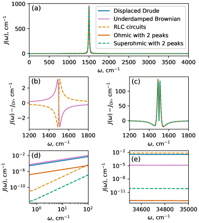
Figure 1: Fit functions for spectral density peaks considered in this study. (a) A single peak at $\omega_{k}=1500$ cm^-1 with width $\gamma_{k}=10$ cm^-1 represented using different functional forms $J_{k}$. The peak intensity (reorganization energy) is set to $\lambda_{k}=20$ cm^-1 so that the peak height is $\sim 1000$ cm^-1 for ease of comparison across the panels. For the two-peak functions $\omega_{k1}=\omega_{k2}=\omega_{k}$, $\Lambda_{2p,k}=\lambda_{k}$ and $\gamma_{k1}=\gamma_{k2}=2\gamma_{k}$. The range of frequencies shown from 0 to $4000$ cm^-1 covers most chemical environments. (b-c) difference of each peak shown in (a) with respect to the displaced Drude oscillator peak. (d) log-log plot of the low frequency tail (up to $200$ cm^-1) of each functional form shown in (a). (e) semilog plot of the high-frequency tail around $35,000$ cm^-1.

II.3 Model system

For simplicity we consider a two level system model of a molecule in aqueous solution. We use electronic parameters as well as the SD obtained for thymine in aqueous solution.[47] However, we emphasize that this is not done to faithfully describe the dynamics of thymine, but rather to make the model parameters realistic. If accurate description of thymine was our goal instead, we would need to account for the conical intersection, that leads to fast ($\sim 400$ fs) population relaxation in the lab.[54]

The parameters for model Hamiltonian (Eq. (4)) are obtained as follows: The energy gap between two levels $\Omega=35,650$ cm^-1 ($4.42$ eV) is extracted from experimenal absorption spectrum of thymine in aqueous solution.[55] We construct the bath using the recently reported SD parameters obtained for thymine in aqueous solution based on resonance Raman experiments.[47] While these parameters are obtained in the pure dephasing limit, we wish to explore the regime where bath-assisted population relaxation is possible as well. We therefore couple the bath via both $\sigma_{z}$ with $\alpha_{z}=0.37$ and $\sigma_{x}$ with $\alpha_{x}=0.34$. The precise choice of coefficients is somewhat arbitrary, but to allow for both dephasing and population relaxation they are chosen to be of comparable magnitude. We use the frequencies and reorganization energies obtained in Ref. 47 (see Table 1).

The resonance Raman experiments do not inform the widths of the peaks $\gamma_{k}$, so we have to make a reasonable choice. The simplest option would be to pick a single width (say 10 $\mathrm{cm}^{-1}$) for all the peaks in the spectral density. This works well for the displaced Drude oscillator, underdamped Brownian, and the RLC circuit functional forms, where intensity of each peak is controlled by the corresponding reorganization energy parameter $\lambda_{k}$. However, for ohmic and superohmic 2-peak functions reorganization energy parameter $\Lambda_{2p,k}$ sets the total peak intensity of a pair of peaks (Eqs. 25-26). The peak widths in Table 1 are chosen (as described in Appendix A) to ensure that the Ohmic 2-peak functions yield individual peak intensities shown in Table 1.

Table 1: Spectral density parameters for our model system. The first two columns are values for thymine obtained from Ref. 47, the third is constructed based on the behavior of Ohmic 2-peak function as described in the main text.

Feature	$\omega_{k}$, cm-1	$\lambda_{k}$, cm-1	$\gamma_{k}$, cm-1
Solvent	0	715.7	54.5
Peak 1	1663	330	10
Peak 2	1243	161.6	36.55
Peak 3	1416	25.6	10
Peak 4	784	26.5	33.77
Peak 5	1376	186	10
Peak 6	1193	77.3	32.01
Peak 7	665	31.9	10
Peak 8	442	14.9	48.46

We use all five functional forms presented in Fig. 1 to include the eight modes (peaks) of the spectral density, resulting in five similar SDs (see Fig. 2). The solvent is included via DL functional form (i.e., setting $\omega_{k}=0$ in Eq. (11)) in each of the five spectral densities. Because the low-frequency range of the spectral density is dominated by this DL solvent feature, this ensures that it is virtually identical for the five SDs we are testing. The SD peaks appear between $\sim 300$ cm^-1 and $\sim 4000$ cm^-1. Here the SD’s obtained with single-peak functional forms (displaced Drude, the UBO and the RLC circuit) display nearly perfect agreement in the vicinity of each peak, while deviating slightly more at the peak edges. The tallest peaks of the SD extend to $J(\omega_{2})\approx 13,000$ and $J(\omega_{1})\approx 18,000$ respectively; we chose not to show the full $y$-range of the SD’s, as this would make the small differences between different functional forms shown on Fig. 2 indistinguishable. The two-peak functions (both Ohmic and Superohmic) visually display more pronounced deviations from the other three, but still match the peak positions, widths and intensities. The high-frequency range of the spectral density is shown on the inset and displays large relative differences between the SD’s constructed with RLC circuit, the displaced Drude and the UBO peaks, as we have seen on panel 1(e). Note that UBO and both of the two-peak functions yield virtually identical high-frequency tails, since all three functional forms decay faster than the DL solvent peak.

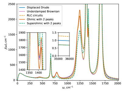
Figure 2: Spectral density built with different functional forms. The parameters are shown in the table 1. The Drude, Brownian and RLC circuit functional forms result in virtually identical spectral density at the peaks with relative difference in intensity in the vicinity of the peak of less than $0.5\%$. The two-peak functions yield more pronounced differences, but overall still adequately approximate the spectral density peaks. The left inset zooms in to the range of frequencies of $1340-1440$ cm^-1, where the peaks are congested; the right inset shows the high-frequency tails in the vicinity of electronic transition frequency $\Omega=35650$ cm^-1.

The simulation is initialized in the product state $\rho(0)=\rho_{s}(0)\otimes\rho_{b}^{\beta}$, where $\rho_{s}(0)=\frac{(\ket{0}+\ket{1})(\bra{0}+\bra{1})}{2}$ is the reduced density matrix of the system at initial time and the bath is initially in thermal state at $300$ K. We integrate the master equation obtained based on time-dependent variational principle using the 4^th order Runge-Kutta integrator with the 5^th order error estimator, also known as the Dormand-Prince algorithm.[56] The timestep is set by the absolute and relative tolerance bounds of $10^{-8}$ and $10^{-5}$ respectively. We use the hierarchy cutoff of $25$ for each HEOM term, and add $8$ low temperature correction Padé terms.[57]

III Results and Discussion

We present the HEOM simulation results over $0.5$ ps at room temperature ($T=300$ K) in Fig. 3.

III.1 Dephasing dynamics

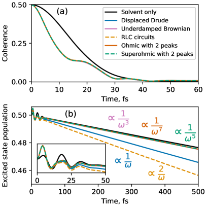
Figure 3: Dynamics of the model system in water using different spectral density basis functions. (a) Dephasing is insensitive to the choice of the spectral density basis functions. (b) Population relaxation is dominated by the high-frequency tails of the spectral density (SD). The color-coded rates of decay of SD peaks are shown for the different functional forms. Number 2 in the numerator of the RLC circuit scaling is to emphasize that it has a prefactor that’s double that of the displaced Drude oscillators (see Eq. (19)). The inset shows that even at early times (after $\sim 25$ fs) the population dynamics deviates significantly depending on the choice of the functional form of SD peaks.

We first focus on the dephasing in the system, shown in Fig. 3a, where the absolute value of the off-diagonal element of the reduced density matrix of the system is plotted as a function of time with different functional forms of the SD peaks. The solvent alone (solid black curve in Fig. 3a) sets dephasing at $\sim 30$ fs. Inclusion of the eight vibrational modes in addition to the DL solvent feature increases the initial dephasing rate, but also introduces additional structure to the dephasing dynamics. More precisely, addition of sharp peaks in the range of frequencies between $\sim 300$ cm^-1 and $\sim 2000$ cm^-1 results in recurrences at $\sim 20$ fs and $\sim 35$ fs, that are not present with solvent-only DL bath. All of these observations echo the findings presented in Ref. 47.

More significantly for this study, the dephasing is insensitive to the choice of the functional form of the vibrational modes in the SD, at least for the five functional forms we tested. The dephasing dynamics up to $\sim 20$ fs is determined by the peak positions, widths, and intensities[47] - all of which are the same for all the functional forms tested. At later times the decay of coherence is determined by the low-frequency end of the spectral density. Even though different functional forms have different low-frequency behaviors (see Eqs. (12), (15), (18) and (21)), their difference in contribution to the low-frequency end of the SD is masked by the DL solvent feature, which dominates in this frequency range (see Fig. 2).

To summarize, we find that dephasing is insensitive to the precise functional form of the structured vibrational peaks in condensed phase dynamics both at early times (controlled by molecular vibrations) and at later times (controlled by the solvent).

III.2 Population relaxation

Population relaxation (Fig. 3b) is about 3 orders of magnitude slower than dephasing for our model system. This corresponds to a typical nonradiative relaxation time of $1$ to $100$ ps for molecules in solution in the absence of near-resonant transition pathway, for example due to the presence of conical intersection. The solvent alone causes excited state population to decay with a lifetime (inverse of exponential decay rate) of $10.5$ ps. We observe that the rate of population relaxation is in some cases increased significantly by the addition of sharp peaks in the range of frequencies between $\sim 300$ cm^-1 and $\sim 2000$ cm^-1. The key finding of this study is that this effect differs significantly depending on the functional form chosen to represent the peaks. Addition of the RLC circuit peaks yields the fastest population decay with lifetime of $5.4$ ps, followed by the displaced Drude oscillator peaks with the lifetime of $7.0$ ps. Brownian and 2-peak Ohmic functions yield similar population lifetimes of $9.8$ ps, just a little faster than that caused by only the DL solvent feature.

To explain these differences we refer back to Fig. 1. The different functional forms to represent each peak in the SD have identical reorganization energies, peak widths and characteristic frequencies, resulting in tiny absolute deviations in the vicinity of the peaks (panels a,b). Yet, these small differences in the functional form of the peaks affect population relaxation rates significantly. We interpret this to be caused by the large relative differences in the high-frequency tails of the five functional forms. The population relaxation rate within Born-Markov approximation[58] is primarily determined (Eq. (24)) by the SD value in the vicinity of the frequency of electronic transition $J(\Omega)$. For the model system we study $\Omega=35650$ cm^-1. The Brownian and 2-peak Ohmic as well as superohmic tails decay quickly (as $\omega^{-3}$, $\omega^{-7}$ and $\omega^{-5}$ respectively, see Eqs. (16) and (22)). For these functional form choices the decay rate at the high-frequency end of the spectrum is higher than that of the DL solvent feature, which decays as $\omega^{-1}$, see Eq. (13). Therefore, the presence of these peaks does not significantly influence the high-frequency tails of the overall SD (see the right inset of Fig. 2), yielding the population lifetime that is only marginally smaller than the $10.5$ ps mark dictated by the solvent alone. This result is expected from mathematical considerations, but counter-intuitive and perhaps that’s why unappreciated in quantum dynamics community. To reiterate, the DL functional form used ubiquitously to represent the low-frequency solvent features in the spectral density not only determines the overall timescale for dephasing, but also has a dominant effect on the overall rate of population relaxation over molecular vibrations when they are represented in the SD via UBO functional form, as is customary.

In contrast to UBO, both the displaced Drude oscillator and the RLC circuit functional forms have peak tails that decay as $\omega^{-1}$, the same rate as the solvent feature. Therefore, vibrations represented with these functional forms can have significant contribution to the overall SD at the high-frequency end of the spectrum. The relative importance of the solvent vs vibrations represented with either Drude or RLC functional forms depends also on the frequency of electronic transition, positions of vibrational peaks, and the difference between both reorganization energies and peak widths of the solvent vs vibrations. Note that the RLC circuits yield faster decay rate as compared to the displaced Drude oscillators because the prefactor of the dominant ($\omega^{-1}$) term at high frequency is two times larger for the former (see the inset of Fig. 2 and Eqs. (13), (19)).

Thus, accurate calculations of slow electronic population relaxation require the precise functional form of the vibrational peaks in addition to the standard peak parameters (widths, positions and intensities). The latter can be obtained experimentally[47, 45, 46] or computationally,[44, 42, 43] while extracting the former from noisy data appears unfeasible at present. Moreover, even if the precise functional form is known, its representation within the numerically exact simulation can be challenging. For example, discretization of the SD or a high-frequency cutoff can introduce error from mishandling the high-frequency end of the SD. Additionally, efficiency considerations within HEOM calculations limit the choice of functional forms of the peaks. Finally, quantum analog simulator devices rely on physical processes to construct the bath, which set the functional form of the simulatable SD peaks. We suggest a recipe to account for the difference between the target and the simulatable SD functional forms in the following section.

III.3 Accounting for different SD tails

Absence of high-frequency (>$10,000$ cm^-1) features in the SD ensures a separation of timescales by 1-3 orders of magnitude between fast dephasing and slow population relaxation. This timescale separation means that the two processes are (essentially) independent. In this limit the differences in population relaxation rates due to the different functional forms in the SD peaks can be accounted for using Eq. (23).

$$p_{\text{target}}(t)\approx p_{eq}+\left(p_{\text{source}}(t)-p_{eq}\right)e^{-(\gamma_{\text{target}}-\gamma_{\text{source}})t}.$$ (23)

Here $p(t)$ is the population of excited state as a function of time of the (known) source and the (unknown) target, which differ only by the functional form of the SD peaks, $p_{eq}=p_{\text{source}}(\infty)=p_{\text{target}}(\infty)$ is the population at thermal equilibrium, and $\gamma$ is the overall population decay rate,

$$\gamma=2\pi\alpha_{x}^{2}J(\Omega)\coth{\left(\frac{\beta\hbar\Omega}{2}\right)}$$ (24)

obtained for both source and target within Born-Markov approximation (Eq. (24)).[58] This rate only depends on temperature, the frequency of electronic transition $\Omega$ and the value of the spectral density at that frequency. Eq. (23) is strictly true only when the source and the target only differ by the overall population decay rate and this difference grows exponentially with time. However, we find it to be an accurate approximation as long as the population relaxation is much slower than dephasing. We derived Eq. (23) for population relaxation obtained via Lindblad equation (see Appendix B), which predicts a simple exponential decay of initial condition to approach thermal equilibrium. For our model system the Lindblad prediction fails at short times, but accurately captures the long-time dynamics and approaches the exact (thermal equilibrium) result $p_{eq}$ as time tends to infinity. This suggests that we can use Eq. (23) together with population relaxation rates calculated based on Eq. (24) to accurately approximate the long-time trends in population relaxation dynamics for any known SD.

This is a useful result in the context of the recently proposed quantum analog simulator device,[38] which uses gate defined double quantum dots and the series of RLC circuits to simulate the system and bath parts of the spin-boson problem. As noted by the authors, the use of RLC circuits to represent the SD of the bath yields functional form of Eq. (17), which is similar (but not identical) to the UBO functional form (Eq. (14)). The ability to establish a simple connection between the functional form obtained from RLC circuits in quantum analog simulators and other target functional forms of the SD peaks is required to simulate systems, whose spectral density peaks do not decay as $\omega^{-1}$.

We illustrate this by taking the result of the HEOM simulation with RLC circuits bath and adjusting it using Eqs. (23) and (24). Fig. 4 shows the RLC circuit results adjusted to reproduce the displaced Drude and UBO peaks as black dotted lines. Recall that the population dynamics with RLC circuit peaks differs substantially from the other two (see Fig. 3); upon adjustment via Eq. (23) we recover excellent agreement with both target HEOM results. Note that the early-time accuracy of the adjusted result does not suffer from the inability of the Lindblad equation (used to derive Eq. (23)) to capture early-time oscillations in excited state population. While early-time dynamics of both target and source is not purely exponential, the oscillations are accurately captured by either of the functional forms, leaving only the overall population decay rate to be adjusted by Eq. (23).

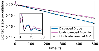
Figure 4: RLC circuit result adjusted using Eq. (23) to reproduce excited state population dynamics with displaced Drude and uderdamped Brownian functional forms of the peaks. The inset shows perfect agreement at early times (first $50$ fs).

IV Conclusions and Implications

We show that the rate of slow nonradiative relaxation is sensitive to the functional form of the peaks used to represent spectral density in numerically exact simulations. More precisely, the high-frequency range of the spectral density is determined by the tails of the peaks. Therefore, functions whose high-frequency tails decay slowly yield faster decay of electronic excitation. This finding has several important implications for using exact quantum dynamics simulations to obtain quantitatively accurate dynamics. Firstly, the methods that truncate the spectral density at high frequency will completely miss this phenomenon. Secondly, proper care needs to be taken to discretize the high-frequency range of the spectrum for the methods that require discretization. Thirdly, we reveal that the Drude-Lorenz solvent feature sets the overall timescale for the population relaxation if the underdamped Brownian functional form is chosen to represent vibrational peaks.

We give a simple recipe to adjust for this difference in decay rates of high-frequency spectral density tails and discuss its application in analog simulation when the precise functional form of the target peaks is unattainable on the device. The adjustment yields accurate target dynamics when the timescales of dephasing and population relaxation are separated and requires no additional information beyond the spectral densities of the simulator and the target.

Appendix A 2-peak SD functions

The normalization constants for the two-peak spectral density basis functions are presented below. We show the simulations only for the Ohmic (Eq. 25) and the superohmic (Eq. 26) cases in Fig. 3.

$$\Lambda_{1,k} =\frac{\Lambda_{2p,k}\prod_{i=\{k_{1},k_{2}\}}\gamma_{i}(\omega_{i}^{2}+\gamma_{i}^{2})(\omega_{i}-\omega_{j}+\gamma_{i})}{\sum_{i=\{k_{1},k_{2}\},j\neq i}\gamma_{i}\left(\gamma_{i}^{2}+4\gamma_{j}^{2}+\omega_{i}^{2}\right)}$$ (25)

$$\Lambda_{3,k} =\frac{\Lambda_{2p,k}\prod_{i=\{k_{1},k_{2}\}}\gamma_{i}}{\sum_{i=\{k_{1},k_{2}\}}\gamma_{i}}$$ (26)

$$\Lambda_{5,k} =\frac{\Lambda_{2p,k}\prod_{i=\{k_{1},k_{2}\}}\gamma_{i}}{\sum_{i=\{k_{1},k_{2}\},j\neq i}\gamma_{i}(\omega_{j}^{2}+\gamma_{j}^{2})}$$ (27)

$$\Lambda_{7,k} =\frac{\Lambda_{2p,k}\prod_{i=\{k_{1},k_{2}\}}\gamma_{i}}{\sum_{i=\{k_{1},k_{2}\},j\neq i}\gamma_{i}\left(4\gamma_{i}^{2}\gamma_{j}^{2}+4\gamma_{j}^{2}\omega_{j}^{2}+(\omega_{j}^{2}+\gamma_{j}^{2})^{2}\right)}$$ (28)

$$\Lambda_{2p,k} =\frac{4(\lambda_{k_{1}}+\lambda_{k_{2}})}{\pi}\left((\omega_{k_{1}}+\omega_{k_{2}})^{2}+(\gamma_{k_{1}}-\gamma_{k_{2}})^{2}\right)\left((\omega_{k_{1}}-\omega_{k_{2}})^{2}+(\gamma_{k_{1}}+\gamma_{k_{2}})^{2}\right)$$ (29)

To set the peak widths in Table 1 we work backwards from the functional form of the Ohmic 2-peak functions (Eq. (20)) to ensure that resulting spectral densities from all five basis function choices are similar with a realistic choice of widths. We pair up the eight peaks creating pairs (1,2), (3,4) etc., such that the two peaks in each pair do not have significant overlap and also have similar reorganization energy parameter ($\lambda_{k}$). We then set the peak widths of $10$ cm^-1 for the four odd index peaks. The widths for the other four peaks (with even indices) are set such that the reorganization energies of each individual peak of the Ohmic 2-peak SD functions match the reorganization energy parameters $\lambda_{k}$ in Table 1.

Appendix B Derivation of tail adjustment

We derive Eqs. (23) and (24) assuming both the source and target populations follow Lindblad equation.[58] In this case the population of excited electronic state changes follows the rate equation:

$$\dot{p}_{1}(t)=\gamma_{-}p_{0}(t)-\gamma_{+}p_{1}(t),$$ (30)

where $\gamma_{-}$ and $\gamma_{+}$ are the (constant) rates of absorption and total (stimulated plus spontaneous) emission given in terms of spectral density as follows:

$$\gamma_{-} = \gamma(-\Omega)=\frac{2\pi\alpha_{x}^{2}J(\Omega)}{e^{\beta\hbar\Omega}-1}=e^{-\beta\hbar\Omega}\gamma_{+}$$ (31)

$$\gamma_{+} = \gamma(+\Omega)=\frac{2\pi\alpha_{x}^{2}J(\Omega)}{1-e^{-\beta\hbar\Omega}}=2\pi\alpha_{x}^{2}J(\Omega)+\gamma_{-}$$ (32)

After elimination of $p_{0}(t)$ from Eq. (30) using $p_{0}(t)+p_{1}(t)=1$ (i.e., ground and excited electronic state populations add up to 1), the equation becomes

$$\dot{p}_{1}(t)=\gamma_{-}[1-p_{1}(t)]-\gamma_{+}p_{1}(t)=\gamma_{-}-\gamma p_{1}(t),$$ (33)

where $\gamma=\gamma_{-}+\gamma_{+}$. Taking the following anzatz:

$$p_{1}(t)=ce^{-bt}+d$$ (34)

with $c$ set by initial condition as $c=p_{1}(0)-d$. Plugging it into Eq. (33):

$$-bce^{-bt}=\gamma_{-}-\gamma ce^{-bt}-\gamma d,$$

so $b=\gamma$ and $d=\frac{\gamma_{-}}{\gamma}=\frac{e^{-\beta\hbar\Omega}}{1+e^{-\beta\hbar\Omega}}=p_{1}(\infty)=p_{1}^{eq}$. Thus,

$$p_{1}(t)=[p_{1}^{0}-p_{1}^{eq}]e^{-\gamma t}+p_{1}^{eq},$$ (35)

where $p_{1}^{0}=p_{1}(0)$ is the initial population of the excited state.

To derive Eq. (23) we write Eq. (35) for both source and target, keeping in mind that initial and final excited state populations of source and target are equal, i.e. $p_{\text{target}}^{0}=p_{\text{source}}^{0}=p_{0}$ and $p_{\text{target}}^{eq}=p_{\text{source}}^{eq}=p_{eq}$

$$p_{\text{target}}(t) = [p_{\text{target}}^{0}-p_{\text{target}}^{eq}]e^{-\gamma_{\text{target}}t}+p_{\text{target}}^{eq}$$ (36)

$$= [p_{0}-p_{eq}]e^{-\gamma_{\text{target}}t}+p_{eq}$$

$$= p_{\text{source}}(t)e^{-[\gamma_{\text{target}}-\gamma_{\text{source}}]t}+p_{eq}\left[1-e^{-[\gamma_{\text{target}}-\gamma_{\text{source}}]t}\right]$$

$$= p_{eq}+\left[p_{\text{source}}(t)-p_{eq}\right]e^{-[\gamma_{\text{target}}-\gamma_{\text{source}}]t}$$

Finally, Eq. (24) follows from Eq. (31) as

$$\gamma=\gamma_{-}+\gamma_{+}=2\pi\alpha_{x}^{2}J(\Omega)\coth{\left(\frac{\beta\hbar\Omega}{2}\right)}$$ (37)

References

- Zadrozny et al. [2015] J. M. Zadrozny, J. Niklas, O. G. Poluektov, and D. E. Freedman, “Millisecond Coherence Time in a Tunable Molecular Electronic Spin Qubit,” ACS Cent. Sci. 1, 488–492 (2015).
- Cao et al. [2020] J. Cao, R. J. Cogdell, D. F. Coker, H.-G. Duan, J. Hauer, U. Kleinekathofer, T. L. C. Jansen, T. Mancal, R. J. D. Miller, J. P. Ogilvie, V. I. Prokhorenko, T. Renger, H.-S. Tan, R. Tempelaar, M. Thorwart, E. Thyrhaug, S. Westenhoff, and D. Zigmantas, “Quantum biology revisited,” Sci. Adv. 6, eaaz4888 (2020).
- Aprahamian [2020] I. Aprahamian, “The Future of Molecular Machines,” ACS Cent. Sci. 6, 347–358 (2020).
- Meyer, Manthe, and Cederbaum [1990] H. D. Meyer, U. Manthe, and L. S. Cederbaum, “The multi-configurational time-dependent Hartree approach,” Chem. Phys. Lett. 165, 73–78 (1990).
- Worth et al. [2008] G. A. Worth, H. D. Meyer, H. Köppel, L. S. Cederbaum, and I. Burghardt, “Using the MCTDH wavepacket propagation method to describe multimode non-adiabatic dynamics,” Int. Rev. Phys. Chem. 27 (2008), 10.1080/01442350802137656.
- Wang and Thoss [2003] H. Wang and M. Thoss, “Multilayer formulation of the multiconfiguration time-dependent Hartree theory,” J. Chem. Phys. 119, 1289–1299 (2003).
- White and Feiguin [2004] S. R. White and A. E. Feiguin, “Real-Time Evolution Using the Density Matrix Renormalization Group,” Phys. Rev. Lett. 93, 076401 (2004).
- Chin et al. [2010] A. W. Chin, Á. Rivas, S. F. Huelga, and M. B. Plenio, “Exact mapping between system-reservoir quantum models and semi-infinite discrete chains using orthogonal polynomials,” J. Math. Phys. 51 (2010), 10.1063/1.3490188.
- Zhou et al. [2016] N. Zhou, L. Chen, Z. Huang, K. Sun, Y. Tanimura, and Y. Zhao, “Fast, Accurate Simulation of Polaron Dynamics and Multidimensional Spectroscopy by Multiple Davydov Trial States,” J. Phys. Chem. A 120 (2016), 10.1021/acs.jpca.5b12483.
- Cederbaum, Gindensperger, and Burghardt [2005] L. S. Cederbaum, E. Gindensperger, and I. Burghardt, “Short-time dynamics through conical intersections in macrosystems,” Phys. Rev. Lett. 94 (2005), 10.1103/PhysRevLett.94.113003.
- Wang and Thoss [2007] H. Wang and M. Thoss, “Quantum dynamical simulation of electron-transfer reactions in an anharmonic environment,” J. Phys. Chem. A 111, 10369–10375 (2007).
- Hu, Gu, and Franco [2018] W. Hu, B. Gu, and I. Franco, “Lessons on electronic decoherence in molecules from exact modeling,” J. Chem. Phys. 148, 134304 (2018).
- Prior et al. [2010] J. Prior, A. W. Chin, S. F. Huelga, and M. B. Plenio, “Efficient simulation of strong system-environment interactions,” Phys. Rev. Lett. 105 (2010), 10.1103/PhysRevLett.105.050404.
- Tanimura [1990] Y. Tanimura, “Nonperturbative Expansion Method for a Quantum System Coupled to a Harmonic-Oscillator bath,” Phys. Rev. A 41, 6676–6687 (1990).
- Ishizaki and Fleming [2009] A. Ishizaki and G. R. Fleming, “Unified treatment of quantum coherent and incoherent hopping dynamics in electronic energy transfer: Reduced hierarchy equation approach,” J. Chem. Phys. 130, 234111–234111 (2009).
- Tang et al. [2015] Z. Tang, X. Ouyang, Z. Gong, H. Wang, and J. Wu, “Extended hierarchy equation of motion for the spin-boson model,” J. Chem. Phys. 143, 224112 (2015).
- Chen and Franco [2024] X. Chen and I. Franco, “Bexcitonics: Quasi-particle approach to open quantum dynamics,” (2024), arxiv:2401.11049 [physics, physics:quant-ph] .
- Makri and Makarov [1995] N. Makri and D. E. Makarov, “Tensor propagator for iterative quantum time evolution of reduced density matrices. I. Theory,” J. Chem. Phys. 102, 4600–4610 (1995).
- Makri [2014] N. Makri, “Blip decomposition of the path integral: Exponential acceleration of real-time calculations on quantum dissipative systems,” J. Chem. Phys. 141, 134117 (2014).
- Strathearn et al. [2018] A. Strathearn, P. Kirton, D. Kilda, J. Keeling, and B. W. Lovett, “Efficient Non-Markovian Quantum Dynamics Using Time-Evolving Matrix Product Operators,” Nat. Commun. 9, 3322 (2018).
- Makri [2021] N. Makri, “Small Matrix Path Integral for Driven Dissipative Dynamics,” J. Phys. Chem. A 125, 10500–10506 (2021).
- Lambert and Makri [2012a] R. Lambert and N. Makri, “Quantum-classical path integral. I. Classical memory and weak quantum nonlocality,” J. Chem. Phys. 137, 22A552 (2012a).
- Lambert and Makri [2012b] R. Lambert and N. Makri, “Quantum-classical path integral. II. Numerical methodology,” J. Chem. Phys. 137, 22A553 (2012b).
- Kundu and Makri [2020] S. Kundu and N. Makri, “Real-Time Path Integral Simulation of Exciton-Vibration Dynamics in Light-Harvesting Bacteriochlorophyll Aggregates,” J. Phys. Chem. Lett. 11, 8783–8789 (2020).
- Feynman and Vernon [1963] R. Feynman and F. Vernon, “The theory of a general quantum system interacting with a linear dissipative system,” Ann. Physics 24, 118–173 (1963).
- Leggett et al. [1987] A. J. Leggett, S. Chakravarty, A. T. Dorsey, M. P. A. Fisher, A. Garg, and W. Zwerger, “Dynamics of the dissipative two-state system,” Rev. Modern Phys. 59, 1–85 (1987).
- Makri [1999] N. Makri, “The Linear Response Approximation and Its Lowest Order Corrections: An Influence Functional Approach,” J. Phys. Chem. B 103, 2823–2829 (1999).
- Chandler [1987] D. Chandler, Introduction to Modern Statistical Mechanics (Oxford University Press, 1987).
- Kundu, Dani, and Makri [2022] S. Kundu, R. Dani, and N. Makri, “B800-to-B850 relaxation of excitation energy in bacterial light harvesting: All-state, all-mode path integral simulations,” J. Chem. Phys. 157, 15101–15101 (2022).
- Lambert et al. [2023] N. Lambert, T. Raheja, S. Cross, P. Menczel, S. Ahmed, A. Pitchford, D. Burgarth, and F. Nori, “QuTiP-BoFiN: A bosonic and fermionic numerical hierarchical-equations-of-motion library with applications in light-harvesting, quantum control, and single-molecule electronics,” Phys. Rev. Research 5, 013181 (2023).
- Gelin, Borrelli, and Chen [2021] M. F. Gelin, R. Borrelli, and L. Chen, “Hierarchical Equations-of-Motion Method for Momentum System-Bath Coupling,” J. Phys. Chem. B 125 (2021), 10.1021/acs.jpcb.1c02431.
- Yan [2019] Y. A. Yan, “Stochastic simulation of anharmonic dissipation. II. Harmonic bath potentials with quadratic couplings,” J. Chem. Phys. 150 (2019), 10.1063/1.5052527.
- Torrontegui and Kosloff [2016] E. Torrontegui and R. Kosloff, “Activated and non-activated dephasing in a spin bath,” New J. Phys. 18 (2016), 10.1088/1367-2630/18/9/093001.
- Kosloff [2019] R. Kosloff, “Quantum thermodynamics and open-systems modeling,” J. Chem. Phys. 150 (2019), 10.1063/1.5096173.
- Hu, Xia, and Kais [2020] Z. Hu, R. Xia, and S. Kais, “A Quantum Algorithm for Evolving Open Quantum Dynamics on Quantum Computing Devices,” Sci. Rep. 10, 3301 (2020).
- Wang et al. [2023] Y. Wang, E. Mulvihill, Z. Hu, N. Lyu, S. Shivpuje, Y. Liu, M. B. Soley, E. Geva, V. S. Batista, and S. Kais, “Simulating Open Quantum System Dynamics on NISQ Computers with Generalized Quantum Master Equations,” J. Chem. Theory Comput. 19, 4851–4862 (2023).
- MacDonell et al. [2021] R. J. MacDonell, C. E. Dickerson, C. J. Birch, A. Kumar, C. L. Edmunds, M. J. Biercuk, C. Hempel, and I. Kassal, “Analog quantum simulation of chemical dynamics,” Chem. Sci. 12, 9794 (2021).
- Kim et al. [2022] C. W. Kim, J. M. Nichol, A. N. Jordan, and I. Franco, “Analog Quantum Simulation of the Dynamics of Open Quantum Systems with Quantum Dots and Microelectronic Circuits,” PRX Quantum 3, 040308 (2022).
- Note [1] Of course, in practice even within the domain of applicability of PI and HEOM methods we are limited by available computational resources, as well as by numerical instabilities.
- May and Kühn [2011] V. May and O. Kühn, Charge and Energy Transfer Dynamics in Molecular Systems (Wiley VCH Verlag GmbH, 2011).
- Ritschel and Eisfeld [2014] G. Ritschel and A. Eisfeld, “Analytic representations of bath correlation functions for ohmic and superohmic spectral densities using simple poles,” J. Chem. Phys. 141, 94101–94101 (2014).
- Olbrich et al. [2011] C. Olbrich, J. Strümpfer, K. Schulten, and U. Kleinekathöfer, “Theory and Simulation of the Environmental Effects on FMO Electronic Transitions,” J. Phys. Chem. Lett. 2, 1771–1776 (2011).
- Damjanović et al. [2002] A. Damjanović, I. Kosztin, U. Kleinekathöfer, and K. Schulten, “Excitons in a photosynthetic light-harvesting system: A combined molecular dynamics, quantum chemistry, and polaron model study,” Phys. Rev. E 65, 031919 (2002).
- Shim et al. [2012] S. Shim, P. Rebentrost, S. Valleau, and A. Aspuru-Guzik, “Atomistic Study of the Long-Lived Quantum Coherences in the Fenna-Matthews-Olson Complex,” Biophys. J. 102, 649–660 (2012).
- Renger and Marcus [2002] T. Renger and R. A. Marcus, “On the relation of protein dynamics and exciton relaxation in pigment–protein complexes: An estimation of the spectral density and a theory for the calculation of optical spectra,” J. Chem. Phys. 116, 9997–10019 (2002).
- Valleau, Eisfeld, and Aspuru-Guzik [2012] S. Valleau, A. Eisfeld, and A. Aspuru-Guzik, “On the alternatives for bath correlators and spectral densities from mixed quantum-classical simulations,” J. Chem. Phys. 137, 224103 (2012).
- Gustin et al. [2023] I. Gustin, C. W. Kim, D. W. McCamant, and I. Franco, “Mapping Electronic Decoherence Pathways in Molecules,” Proc. Natl. Acad. Sci. 120, e2309987120–e2309987120 (2023).
- Tanimura and Kubo [1989] Y. Tanimura and R. Kubo, “Time evolution of a quantum system in contact with a nearly Gaussian-Markoffian noise bath,” J. Phys. Soc. Jpn. 58, 101–114 (1989).
- Xu et al. [2022] M. Xu, Y. Yan, Q. Shi, J. Ankerhold, and J. T. Stockburger, “Taming Quantum Noise for Efficient Low Temperature Simulations of Open Quantum Systems,” Phys. Rev. Lett. 129, 230601 (2022).
- Ikeda and Scholes [2020] T. Ikeda and G. D. Scholes, “Generalization of the Hierarchical Equations of Motion Theory for Efficient Calculations with Arbitrary Correlation Functions,” J. Chem. Phys. 152, 204101 (2020).
- Liu et al. [2014] H. Liu, L. Zhu, S. Bai, and Q. Shi, “Reduced quantum dynamics with arbitrary bath spectral densities: Hierarchical equations of motion based on several different bath decomposition schemes,” J. Chem. Phys. 140, 134106 (2014).
- Tanimura [2012] Y. Tanimura, “Reduced hierarchy equations of motion approach with Drude plus Brownian spectral distribution: Probing electron transfer processes by means of two-dimensional correlation spectroscopy,” J. Chem. Phys. 137, 22A550 (2012).
- Mukamel [1995] S. Mukamel, Principles of Nonlinear Optical Spectroscopy (Oxford University Press, 1995).
- Erickson et al. [2019] B. A. Erickson, Z. N. Heim, E. Pieri, E. Liu, T. J. Martinez, and D. M. Neumark, “Relaxation Dynamics of Hydrated Thymine, Thymidine, and Thymidine Monophosphate Probed by Liquid Jet Time-Resolved Photoelectron Spectroscopy,” J. Phys. Chem. A 123 (2019), 10.1021/acs.jpca.9b08258.
- Ng et al. [2008] S. Ng, S. Yarasi, P. Brest, and G. R. Loppnow, “Erratum: Initial excited-state structural dynamics of thymine are coincident with the expected photochemical dynamics (Journal of Physical Chemistry A (2007) 111A (5130-5135)),” J. Phys. Chem. A 112 (2008), 10.1021/jp806433h.
- Hairer, Nørsett, and Wanner [2000] E. Hairer, S. Nørsett, and G. Wanner, Solving Ordinary Differential Equations I Nonstiff Problems, 2nd ed. (Springer, Berlin, 2000).
- Hu, Xu, and Yan [2010] J. Hu, R.-X. Xu, and Y. Yan, “Communication: Padé Spectrum Decomposition of Fermi Function and Bose Function,” J. Chem. Phys. 133, 101106 (2010).
- Lidar [2020] D. A. Lidar, “Lecture Notes on the Theory of Open Quantum Systems,” (2020), arxiv:1902.00967 [quant-ph] .