Nonlinearity-induced symmetry breaking in a system of two parametrically driven Kerr-Duffing oscillators

Abstract

We study the classical dynamics of a system comprising a pair of Kerr-Duffing nonlinear oscillators, which are coupled through a nonlinear interaction and subjected to a parametric drive. Using the rotating wave approximation (RWA), we analyze the steady-state solutions for the amplitudes of the two oscillators. For the case of almost identical oscillators, we investigate separately the cases in which only one oscillator is parametrically driven and in which both oscillators are simultaneously driven. In the latter regime, we demonstrate that even when the parametric drives acting on the two oscillators are identical, the system can transition from a stable symmetric solution to a broken-symmetry solution as the detuning is varied.

I Introduction

Nonlinear dynamics of resonantly driven oscillator modes is a very general theme common to many fields of physics, from nanomechanical systems to photonics. In the mechanical context, it has received growing attention in view of metrological applications [1, 2, 3, 4, 5, 6, 7] as well as from a fundamental science perspective. Driven nonlinear nanomechanical systems constitute, in fact, an ideal platform for the investigation of fundamental aspects of nonlinear dynamics and nonequilibrium fluctuations [8, 9, 10, 11]. In photonics, models involving a few resonantly-driven modes coupled by nonlinear processes provide a powerful framework to describe nonlinear optical processes leading to the mixing of different beams and to the generation of new harmonic and/or sub-harmonic components and are at the heart of devices for quantum and/or nonlinear optics applications [12, 13, 14, 15, 16] .

In general, nonlinear coupling between resonant modes is expected to become strong when the ratio between their resonance frequencies is an integer (linear resonance 1:n) or rational (parametric resonance 2:n), viz. the so-called internal resonances [17]. In particular, an interaction of the kind 2:2, also known as cross-Kerr interaction can be described as the oscillations of the first resonator acting as a parametric frequency modulation on the second resonator. When internal resonances are not present, the 2:2 nonlinear interaction can still give a dispersive shift of the mode frequencies, which depends on the oscillation amplitude of the driven mode. Such a dispersive interaction has been observed in a variety of nanomechanical systems, e.g. doubly clamped beams or strings, clamped nano- or microcantilevers, and in doubly clamped, nanomechanical silicon nitride string resonators [18, 19, 20, 21, 22, 23, 24, 25, 26].

In photonics, nonlinear interaction processes are mediated by the nonlinear response of the material medium, in particular second-order $\chi^{(2)}$ and third-order $\chi^{(3)}$ nonlinearities, leading to a variety of phenomena, from optical bistability to parametric amplification and oscillation [12, 14, 13, 27, 15, 16, 28]. In the last decades, growing attention has been paid to systems featuring a complex interplay of several nonlinear phenomena at once and/or well-defined discrete modes [29, 30, 31]. Nowadays, an active frontier is to explore fundamental aspects of non-equilibrium fluctuations around the steady-state of spatially extended systems and shine a light on their relation to fundamental questions of pattern formation in nonlinear systems [32, 33, 34, 35].

In this paper, we investigate a simple model based on two Kerr/Duffing oscillators coupled through nonlinear interaction terms, proportional to the product of the squares of the two amplitudes of the two modes $\sim q_{1}^{2}q_{2}^{2}$. Within the rotating wave approximation (RWA), we analyze the possible stationary paired solutions and their dynamical stability in two scenarios: one where only one of the two modes is parametrically driven, and another where both resonators are driven.

When both resonators are parametrically driven at the same frequency, the paired amplitudes of the two modes show a complex and intriguing behavior which is also characterized by the presence of several instability ranges in the frequency detuning. As a particularly interesting result, we find that when the two resonators have identical parameters and are driven with equal parametric force, the overall symmetry of the system can be spontaneously broken for moderately weak nonlinear interaction. This leads to an intriguing multistability phenomenon, featuring steady states with different amplitudes and phases on the two oscillators.

The article is organized as follows. In Sec. II, we introduce the model and the effective dynamical equations in the rotating frame using the RWA. In Sec. III, we shortly discuss the behavior of the system when both resonators have non-zero oscillation amplitude when only one resonator is driven. In Sec. IV, we start analyzing the most intriguing case when both resonators are simultaneously driven and the emergence of symmetry breaking. In the successive Sec.V and Sec.VI, we respectively give an analytical form for the symmetric solution and, then, a numerical analysis for the broken symmetry case. Conclusions are finally drawn in Sec.VII.

II The system

We introduce the mathematical model that describes two nonlinear parametrically driven resonantors coupled by the dispersive (cross-Kerr) interaction. We consider two resonators with equal damping coefficients and equal self Kerr-Duffing parameters. We refer to the Appendix A for further details.

In the rotating frame and using the RWA, the equations for the complex amplitudes associated with the two resonators oscillating at frequencies $\omega_{d}$ are

$$\frac{\partial z_{1}}{\partial\tau}=iF_{1}\left(z_{1},z_{2}\right)\,,\quad\frac{\partial z_{2}}{\partial\tau}=iF_{2}\left(z_{2},z_{1}\right)$$ (1)

with the functions $F_{n}\left(z_{n},z_{m}\right)$

$$F_{n}\left(z_{n},z_{m}\right) =\left({|z_{n}|}^{2}-\delta\Omega_{n}+i\right)z_{n}+\delta\Omega_{T,n}z_{n}^{*}$$

$$+g\left(2{|z_{m}|}^{2}z_{n}+z_{m}^{2}z_{n}^{*}\right)\,.$$ (2)

for $n=1$ and $m=2$ and viceversa.

Here $\delta\Omega_{n}$ corresponds to the scaled detuning for the resonator $n$ and $\delta\Omega_{T,n}$ is proportional to the strength of the parametric drive. It also corresponds to the (scaled) frequency threshold for the self-sustained oscillatory motion of the resonator $n$ in the limit of vanishing damping and without interaction. The parameter $g$ represents the scaled coupling strength of the nonlinear interaction.

The stationary solution are obtained by requiring $\partial z_{1}/\partial\tau=\partial z_{2}/\partial\tau=0$, namely by solving the two coupled nonlinear equations

$$F_{1}\left(\bar{z}_{1},\bar{z}_{2}\right)=F_{2}\left(\bar{z}_{2},\bar{z}_{1}\right)=0\,.$$ (3)

We analyze the dynamical stability of these solutions by analyzing the small fluctuation around these points $z_{n}\simeq\bar{z}_{n}+\delta z_{n}$, namely, we consider the equations for the vector of the fluctuations

$$\frac{\partial}{\partial\tau}\left(\begin{array}[]{c}\delta z_{1}\\ \delta z_{1}^{*}\\ \delta z_{2}\\ \delta z_{2}^{*}\end{array}\right)=i\left(\begin{array}[]{cccc}a_{1}&b_{1}&c&d\\ -b^{*}_{1}&-a_{1}&-d^{*}&-c\\ c&d&a_{2}&b_{2}\\ -d^{*}&-c&-b_{2}^{*}&-a_{2}\end{array}\right)\left(\begin{array}[]{c}\delta z_{1}\\ \delta z_{1}^{*}\\ \delta z_{2}\\ \delta z_{2}^{*}\end{array}\right)$$ (4)

with the coefficients evaluated at the stationary solutions

$$a_{1} =2{|\bar{z}_{1}|}^{2}-\delta\Omega_{1}+2g{|\bar{z}_{2}|}^{2}+i\,,$$ (5)

$$a_{2} =2{|\bar{z}_{2}|}^{2}-\delta\Omega_{2}+2g{|\bar{z}_{1}|}^{2}+i\,,$$ (6)

$$b_{1} =\bar{z}_{1}^{2}+\delta\Omega_{T,1}+g\bar{z}_{2}^{2}\,,$$ (7)

$$b_{2} =\bar{z}_{2}^{2}+\delta\Omega_{T,2}+g\bar{z}_{1}^{2}\,,$$ (8)

$$c =2g\left(\bar{z}_{1}^{*}\bar{z}_{2}+\bar{z}_{1}\bar{z}_{2}^{*}\right)\,,$$ (9)

$$d =2g\bar{z}_{1}\bar{z}_{2}\,.$$ (10)

When the real parts of all eigenvalues of the matrix appearing in Eq. (4) - including the factor $i$ - are negative, the stationary solution is dynamically stable against noise. In the limit of small damping, which corresponds to neglect the factor $i$ in the coefficients $a_{1}$ and $a_{2}$, the solutions are dynamically stable simply when the real parts of the eigenvalues vanish.

Hereafter we focus our analysis on the strong nonlinear regime in which the motion is dominated by the nonlinear interaction such that we can neglect the damping force, which is valid in the limit $3\kappa A_{n}^{2}/(8\omega_{d})\gg\Gamma$ with $A_{n}$ the amplitude of the oscillatory motion of the resonator $q_{n}(t)=A_{n}\cos(\omega_{d}t+\theta_{n})$, $\kappa$ is the Kerr-Duffiing parameter, $\Gamma$ is the damping and $\omega_{d}$ is half of the drive frequency (see appendix A). This approximation is not valid when we are close to the parametric threshold when the resonator starts to oscillate at frequency $\omega_{d}$ and the amplitude can be small enough to violate the previous condition. However, the effect of the damping is the renormalization of the threshold. Even in the presence of a nonlinear interaction, we have numerically benchmarked that small damping simply results in a minor renormalization or shift of the critical thresholds when new solutions emerge or existing solutions vanish with varying detuning.

Before analyzing the solutions in which both resonators oscillate, $\bar{z}_{1}\neq 0$ and $\bar{z}_{2}\neq 0$, we discuss shortly the simple cases in which one of the two resonators is at rest. We refer to the appendices B, C for a more extended analysis.

First of all, for a single parametrically driven nonlinear resonator (uncoupled case $g=0$), one has the following (stable) steady-state solution for $\bar{z}$: the resonator starts to oscillate at frequency $\omega_{d}$ above the detuning threshold $\delta\Omega>-\delta\Omega_{T,1}$ and it is entirely out of phase with respect to the drive, in the limit of vanishing damping (see appendix B). The trivial solution $\bar{z}^{(0)}_{1}=0$ is unstable in the detuning range $|\delta\Omega|<\delta\Omega_{T,1}$.

When we switch on the interaction, we discuss the stationary pair solutions. In particular, the trivial solution $\left(\bar{z}_{1}=0,\bar{z}_{2}=0\right)$ is still a stationary solution and unstable for $|\delta\Omega_{i}|<\delta\Omega_{T,i}$ as for the case $g=0$. On the other hand, for the pair solutions with the trivial solution for one of the two resonators $\bar{z}_{n}=0$, the equations for $\delta z_{1}$ and $\delta z_{2}$ become decoupled (see Eq. (4), the coefficients $c$ and $d$ vanish) but they are still correlated as the finite value of the amplitude of the driven mode $\bar{z}_{n}$ affects the fluctuation of the second non-driven mode $\delta z_{m}$ and therefore the range of stability can be different from the noninteracting case, see appendix C.

III Finite amplitude solutions for one driven resonator

We now analyze the system when the external drive is applied only to the first resonator $(\delta\Omega_{T,2}=0)$. In appendix D, we give a detailed analysis of this regime, in which we report the analytical solutions in table 1. The different possible solutions are associated with different ranges of the coupling strength $g$, in particular in the ranges $0<g<1/3$, $1/3<g<1$ and $g>1$. We checked that the numerical results are in good agreement with the analytical solutions shown in appendix D.

In short, when only the first mode is driven, the cross-Kerr interaction changes the system’s stability range even when we have the trivial solution for the second non-driven mode. Furthermore, the first resonator can drive the state of the second resonator in an oscillatory motion.

We give an example of results for this regime in Fig. 1 (numerical results) in which we plot stable pair solutions (solid lines) and unstable ones (dashed lines). In particular, we notice that, for the stable solutions, the second non-driven resonator starts to oscillate for a given threshold detuning. This leads to a discontinuity in the amplitude curve of the driven resonator. Changing the parameters of the system, we also find that the curve for the amplitude of the second resonator can have a discontinuity in which the amplitude $\bar{z}_{2}$ has a jump from zero to a finite value.

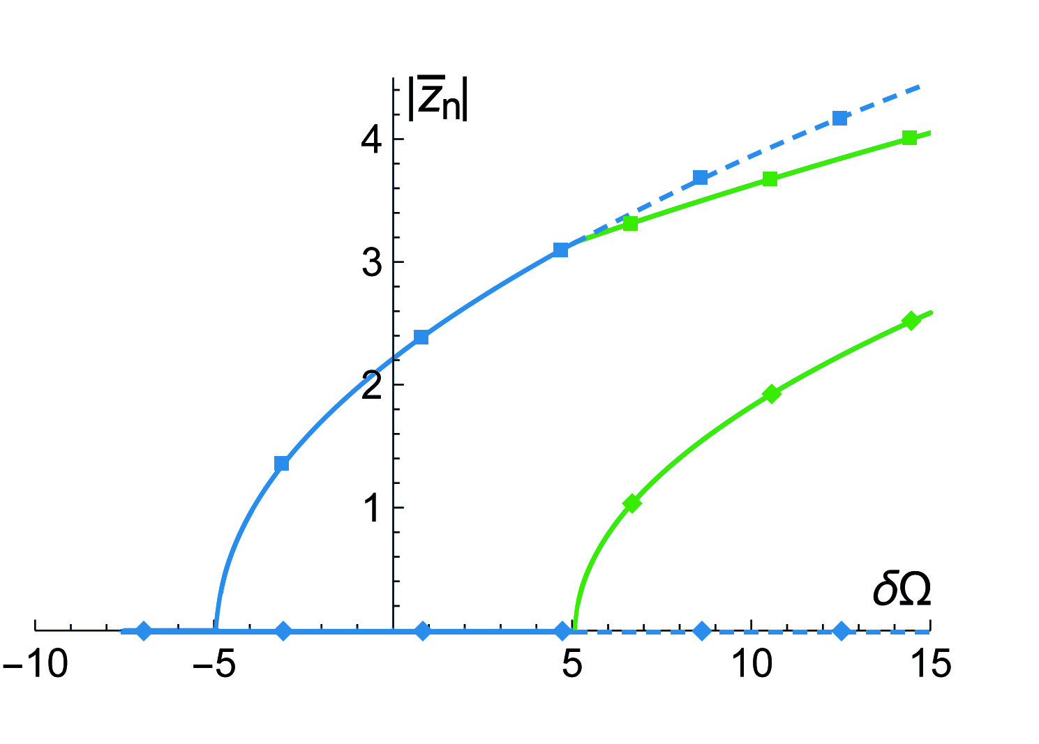
Figure 1: Example of the behavior for a single-driven mode. Legend: The amplitudes of the two different resonators are distinguished by the symbol, i.e., $\blacksquare$ for $|\bar{z}_{1}|$, $\blacklozenge$ for $|\bar{z}_{2}|$. Lines with the same color show solution pairs of the two resonators. Solid lines correspond to stable solutions. Dashed lines correspond to unstable solutions. Parameters: $g=1/2$, $\delta\Omega_{T,1}=5$ and $\delta\Omega_{T,2}=0$. The blue lines show the solution pairs with only one oscillating resonator while the other one is at rest.

IV Finite amplitude solutions for two driven resonators

In this section, we analyze the case of both nonlinear resonators being parametrically driven. We consider the degenerate case, with $\omega_{1}=\omega_{2}$ such that the detuning frequencies are the same $\delta\Omega_{1}=\delta\Omega_{2}=\delta\Omega$.

IV.1 Numerical analysis for asymmetric drive $\delta\Omega_{T,1}\neq\delta\Omega_{T,2}$

We start the analysis when the strengths of the two parametric drives are different $\delta\Omega_{T,1}\neq\delta\Omega_{T,2}$. For this case, we discuss some simple limits, in a qualitative manner, that we have tested numerically and show an example of results.

First of all, in the limit of weak coupling $g\ll 1$, the solutions are connected qualitatively to uncoupled solutions for two noninteracting modes, as expected.

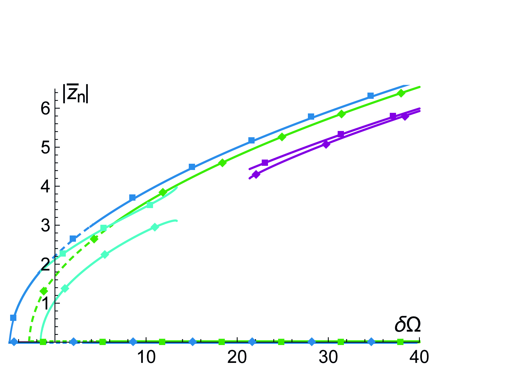
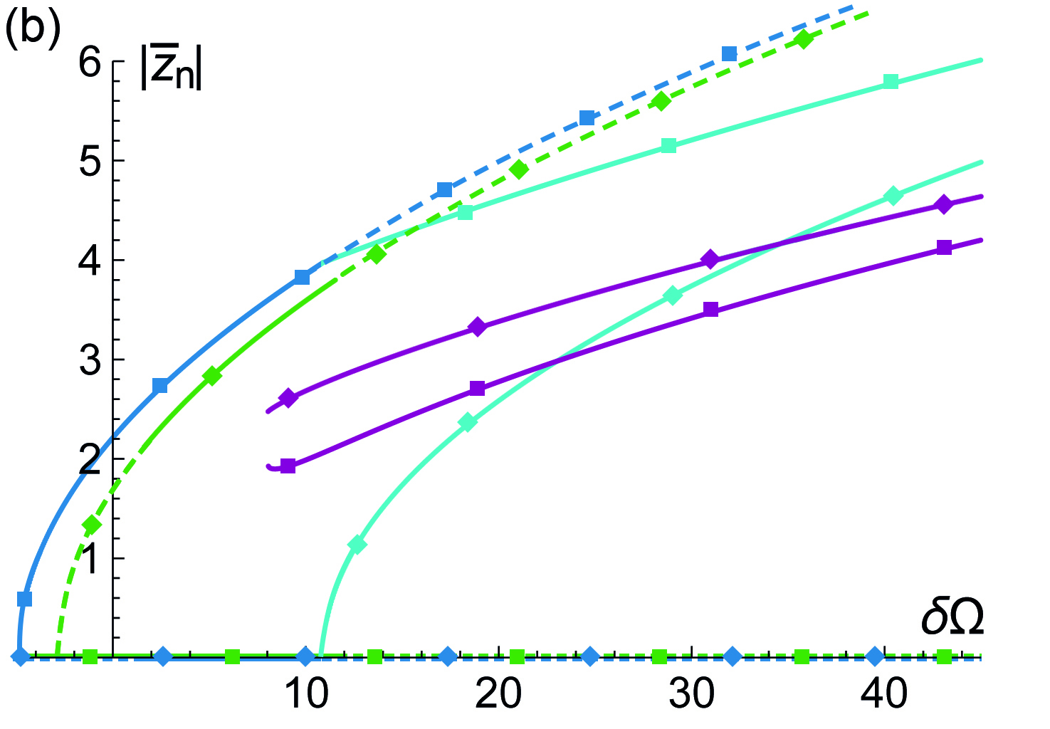
Figure 2: Example of the behavior of the system for two driven modes with different drive strengths. Legend: The amplitudes of the two different resonators are distinguished by the symbol, i.e. $\blacksquare$ for $|\bar{z}_{1}|$, $\blacklozenge$ for $|\bar{z}_{2}|$. Lines with the same color show solution pairs of the two resonators. Solid lines correspond to stable solutions. Dashed lines correspond to unstable solutions. The green and blue lines are the paired solutions with $\bar{z}_{1}=0$ or $\bar{z}_{2}=0$. Parameters: (a) $\delta\Omega_{T,1}=3$, $\delta\Omega_{T,2}=5$, $g=1/8$. (b) $\delta\Omega_{T,1}=10/3$, $\delta\Omega_{T,2}=5$, $g=1/2$.

On the other hand, for $\delta\Omega_{T,1}\gg\delta\Omega_{T,2}$, for moderate force acting on the first resonator $\delta\Omega_{T,1}\gg 1$ and not so small coupling $g$, the solutions are connected qualitatively to ones obtained for the case of a single-driven mode, see Sec. III. One can estimate this regime in the small damping limit in which we have ${|z_{1}|}^{2}\approx\delta\Omega_{T,1}$ at small detuning. Hence the effects of the first resonator dominate on the second drive for $g\delta\Omega_{T,1}\gg\delta\Omega_{T,2}$. In such regime the interaction between the two resonators dominates over the second drive, the amplitude of the second - weakly driven - resonator is determined by its parametric interaction with the first resonator in a way qualitatively similar to the results discussed in Sec. III.

The more interesting regime occurs when the strength of the two drives are comparable, and the interaction strength is also not so small. An example of results in such a regime is shown in Fig. 2 for $g=1/8$ and $g=1/2$. Here the blue and green lines are the paired solutions with $\bar{z}_{2}=0$ or $\bar{z}_{1}=0$, respectively. The solid lines show the stable solutions. As there are many unstable solutions, we include only a few examples of them in the figure corresponding to the dashed lines.

For $g=1/8$ , we have stable solutions of finite amplitudes, $\bar{z}_{1}\neq 0$ and $\bar{z}_{2}\neq 0$, (turquoise lines) up to some detuning, after that they disappear, and two new stable solutions emerge again at larger detuning (purple lines). The system has multistability when we regard the phase since the modulus of the solutions shown in Fig. 2 corresponds to solutions of different phases. One can show that, in total, there are four different paired solutions corresponding to the four possible combinations of the phases.

For the case $g=1/2$, the system shows a multistability even for the modulus, as shown Fig. 2b, in which two paired solutions of different amplitudes (turquoise lines and purple lines) are stable in the same detuning range. In this case, the system admits eight stable paired solutions, e.g. four solutions for a given pair of amplitudes.

IV.2 Numerical analysis for symmetric drive $\delta\Omega_{T,1}=\delta\Omega_{T,2}$

As the most interesting case, we analyze the case in which the strength of the two drives is the same $\delta\Omega_{T,1}=\delta\Omega_{T,2}$. In this case, the system is fully symmetric. An example of results in such a regime is shown in Fig. 3 for $g=1/5$, $g=3/10$ and $g=1/2$, in the limit of negligible damping.

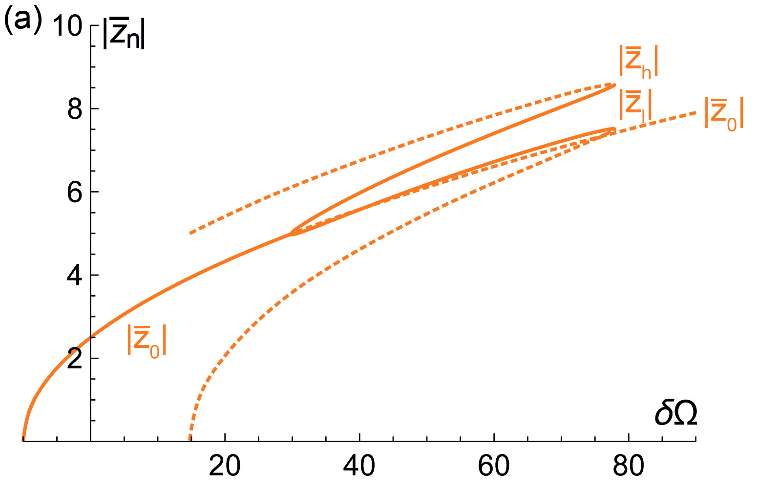
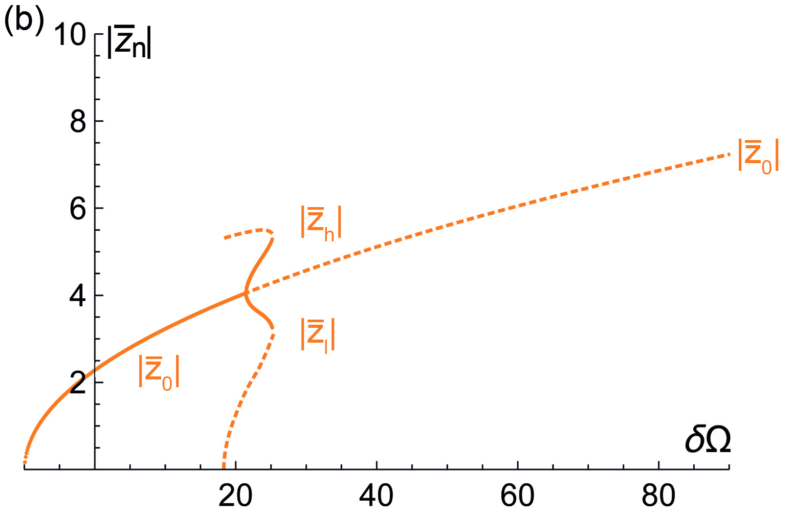
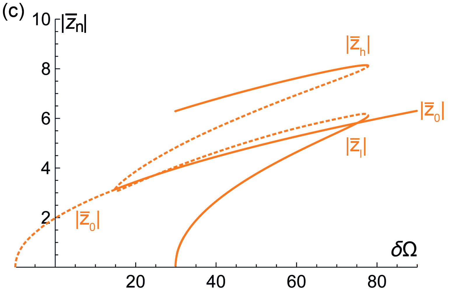
Figure 3: Example of the behavior of the system for two driven modes with symmetric drive. The orange indicates that two solutions overlap/exist with the same amplitude. The solid lines are the stable solutions, whereas the dashed lines correspond to the unstable ones. Parameters: $\delta\Omega_{T,1}=\delta\Omega_{T,2}=10$; (a) $g=1/5$; (b) $g=3/10$; (c) $g=1/2$.

The symmetry of the equations leads to a natural symmetric solution in which the two resonators have the same oscillatory amplitude $|\bar{z}_{1}|=|\bar{z}_{2}|=|\bar{z}_{0}|$. We find that this solution is stable for different ranges, as indicated in Fig. 3. Although the modulus is the same, the system has a multistability related to the combinations of all possible phases of the solutions (similar to the results of the previous section). Denoting the two possible states for each resonator as $|\bar{z}_{0}|e^{i\varphi_{0,+}}$ and $|\bar{z}_{0}|e^{i\varphi_{0,-}}$, we obtain in total four possible solution pairings depending on whether the two resonators have either different or equal phases. They correspond to ($\varphi_{0,+}$,$\varphi_{0,+}$), ($\varphi_{0,+}$,$\varphi_{0,-}$), ($\varphi_{0,-}$,$\varphi_{0,+}$), ($\varphi_{0,-}$,$\varphi_{0,-}$), with $|\varphi_{0,+}-\varphi_{0,-}|=\pi$.

When we increase the coupling, we observe that at $g=1/3$ the region of stability of the symmetric solution changes discontinuously. For $g<1/3$ the symmetric solution is stable from $\delta\Omega>-\delta\Omega_{T}$ up to a critical detuning $\delta\Omega<\delta\Omega_{c,S}$, see Fig. 3a and Fig. 3b, whereas it becomes stable at large detuning $\delta\Omega>\delta\Omega_{c,S}$ for $g>1/3$, see Fig. 3c. We have numerically calculated the critical value $g$ at which the system with broken symmetry switches from the solution types of Fig. 3a and Fig. 3b to the solution types of Fig. 3c, at different values of the drive strength $\delta\Omega_{T}$. Within the range of parameters explored in our numerical solutions, we find that the critical coupling at which the discontinuity occurs is $g_{c}\approx 1/3$ and it is independent of the drive strength $\delta\Omega_{T}$. The latter only affects the critical detunings $\delta\Omega_{c,S}$ at different $g$.

For $g<1/3$, at $\delta\Omega=\delta\Omega_{c,S}$, we have a pitchfork bifurcation of the stable solutions: for $\delta\Omega>\delta\Omega_{c,S}$, the symmetric solution is unstable, and we have a solution with broken symmetry in amplitudes $|\bar{z}_{1}|\neq|\bar{z}_{2}|$, see Fig. 3a and Fig. 3b. For $g>1/3$, the symmetric solution becomes stable for $\delta\Omega>\delta\Omega_{c,S}$ whereas the broken-symmetry solution results are stable at larger detuning, see Fig. 3c, with one of them appearing at finite amplitude in a discontinuous way.

V Symmetric solutions for symmetric drive

In the limit of vanishing damping, the symmetric solutions take the form

$$z_{0}=\pm i\,\frac{\delta\Omega+\delta\Omega_{T}}{1+3g}$$ (11)

where we set $\delta\Omega_{T}=\delta\Omega_{T,1}=\delta\Omega_{T,2}$. Then the coefficients of the matrix associated to the fluctuations Eq. (4) around the stationary points are real and read

$$a =2\left(1+g\right){\left|z_{0}\right|}^{2}-\delta\Omega\,,$$ (12)

$$b =-\left(1+g\right){\left|z_{0}\right|}^{2}+\delta\Omega_{T}\,,$$ (13)

$$c =\pm 4g{\left|z_{0}\right|}^{2}\,,$$ (14)

$$d =\mp 2g{\left|z_{0}\right|}^{2}\,.$$ (15)

with the sign $\pm$ $(\mp)$ depending on the phases of the paired solution, e.g. the same $\bar{z}_{1}=\bar{z}_{2}$ or different phase $\bar{z}_{1}=-\bar{z}_{2}$. Setting $\delta z_{n}=\delta Q_{n}-i\delta P_{n}$ and changing the variables $\delta Q_{\Sigma}=\delta Q_{1}+\delta Q_{2}$, $\delta Q_{\Delta}=\delta Q_{1}-\delta Q_{2}$, $\delta P_{\Sigma}=\delta P_{1}+\delta P_{2}$, $\delta P_{\Delta}=\delta P_{1}-\delta P_{2}$, one can obtain the expansion of the Hamiltonian around the symmetric stable solution as the same of two quadratic Hamiltonian

$$H_{\mathrm{RWA}}^{(2)}=H_{\Sigma}+H_{\Delta}\,.$$ (16)

with

$$H_{\Sigma} =\frac{1}{2}\Omega_{P,\Sigma}\,\,\delta P_{\Sigma}^{2}+\frac{1}{2}\Omega_{Q,\Sigma}\,\,\delta Q_{\Sigma}^{2}\,,$$ (17)

$$H_{\Delta} =\frac{1}{2}\Omega_{P,\Delta}\,\,\delta P_{\Delta}^{2}+\frac{1}{2}\Omega_{Q,\Delta}\,\,\delta Q_{\Delta}^{2}\,.$$ (18)

in which the conjugate variables are $\left(\delta Q_{\Sigma},\delta P_{\Sigma}\right)$ and $\left(\delta Q_{\Delta},\delta P_{\Delta}\right)$ with the following dynamical equations

$$\delta\dot{P}_{\Sigma}=\partial H_{\Sigma}/\partial\delta Q_{\Sigma}\,,\quad\delta\dot{Q}_{\Sigma}=-\partial H_{\Sigma}/\partial\delta\dot{Q}_{\Sigma}\,,$$ (19)

$$\delta\dot{P}_{\Delta}=\partial H_{\Delta}/\partial\delta\dot{Q}_{\Delta}\,,\quad\delta\dot{Q}_{\Delta}=-\partial H_{\Delta}/\delta\dot{P}_{\Delta}\,.$$ (20)

The system is dynamically stable as long as the product of the two coefficients in each quadratic Hamiltonian is positive, namely $\Omega_{P,\Sigma}\Omega_{Q,\Sigma}>0$ and $\Omega_{P,\Delta}\Omega_{Q,\Delta}>0$.

For example, for $\bar{z}_{1}=\bar{z}_{2}$, the coefficients are

$$\Omega_{P,\Sigma} =2\left(\delta\Omega+\delta\Omega_{T}\right)\,,$$ (21)

$$\Omega_{Q,\Sigma} =2\delta\Omega_{T}\,,$$ (22)

and

$$\Omega_{P,\Delta} =2\,\frac{1-3g}{1+3g}\left(\delta\Omega+\delta\Omega_{T}\right)\,,$$ (23)

$$\Omega_{Q,\Delta} =2\,\frac{\delta\Omega_{T}}{1+3g}\left[1-g\left(2\frac{\delta\Omega}{\delta\Omega_{T}}-1\right)\right]\,.$$ (24)

The quadratic Hamiltonian around the stationary point $\bar{z}_{1}=-\bar{z}_{2}$ has a similar form which can be written by exchanging the coefficient $\Omega_{P,\Sigma}$ with $\Omega_{P,\Delta}$ and the coefficient $\Omega_{Q,\Sigma}$ with $\Omega_{Q,\Delta}$.

For positive detuning $\delta\Omega>0$, we observe that only the coefficient Eq. (23) and Eq. (24) can change the sign by varying the detuning and the coupling constant. In particular Eq. (23) is positive for $g<1/3$. The frequency Eq. (24) is always positive in the range $0<g<1$ for for $\delta\Omega<\delta\Omega_{T}/2$ whereas for $\delta\Omega>\delta\Omega_{T}/2$ we have the condition

$$g<\frac{1}{2\frac{\delta\Omega}{\delta\Omega_{T}}-1}\,,\qquad\mbox{for}\quad\delta\Omega>\frac{\delta\Omega_{T}}{2}\,.$$ (25)

In conclusion, when both Eq. (23) and Eq. (24) are positive or negative, the system is stable: the critical line $g_{c}=1/3$ and Eq. (25) determines the stability phase diagram shown in Fig. 5 for the symmetric solution.

VI Broken-symmetry solutions for symmetric drive

We now discuss the behavior of the broken symmetry solutions. At the pitchfork bifurcation, as shown in Fig. 3(a) and Fig. 3(b), we have two stable non-symmetric solutions which we denote $|\bar{z}_{h}|$ and $|\bar{z}_{l}|$. The system has multistability characterized by the possibility of exchanging the amplitudes of the two resonators, i.e. we have a state with $|\bar{z}_{1}|=|\bar{z}_{h}|$ and $|\bar{z}_{2}|=|\bar{z}_{l}|$ and a different state with $|\bar{z}_{1}|=|\bar{z}_{l}|$ and $|\bar{z}_{2}|=|\bar{z}_{h}|$.

Furthermore, even if we fix the modulus of the amplitudes of the two resonators, for example, $|\bar{z}_{1}|=|\bar{z}_{h}|$ and $|\bar{z}_{2}|=|\bar{z}_{l}|$, this state is still characterized by multistability owing to the different phases associated to each solution $\bar{z}_{h}$ and $\bar{z}_{l}$. More explicitly, we have four possible states given by four possible combinations of the phases

$$(1)\qquad\bar{z}_{1}=|\bar{z}_{h}|e^{i\varphi_{h,+}}\,\,\,\,\bar{z}_{2}=|\bar{z}_{l}|e^{i\varphi_{l,+}}\,,$$ (26)

$$(2)\qquad\bar{z}_{1}=|\bar{z}_{h}|e^{i\varphi_{h,+}}\,\,\,\,\bar{z}_{2}=|\bar{z}_{l}|e^{i\varphi_{l,-}}\,,$$ (27)

$$(3)\qquad\bar{z}_{1}=|\bar{z}_{h}|e^{i\varphi_{h,-}}\,\,\,\,\bar{z}_{2}=|\bar{z}_{l}|e^{i\varphi_{l,+}}\,,$$ (28)

$$(4)\qquad\bar{z}_{1}=|\bar{z}_{h}|e^{i\varphi_{h,-}}\,\,\,\,\bar{z}_{2}=|\bar{z}_{l}|e^{i\varphi_{l,-}}\,.$$ (29)

with $|\varphi_{h,+}-\varphi_{h,-}|=|\varphi_{l,+}-\varphi_{l,-}|=\pi$.

We summarize the behavior of the paired solutions in Fig. 4 in which we plot the complex amplitudes of Fig. 3a parametrically as a function of the detuning for the case $g=1/5$.

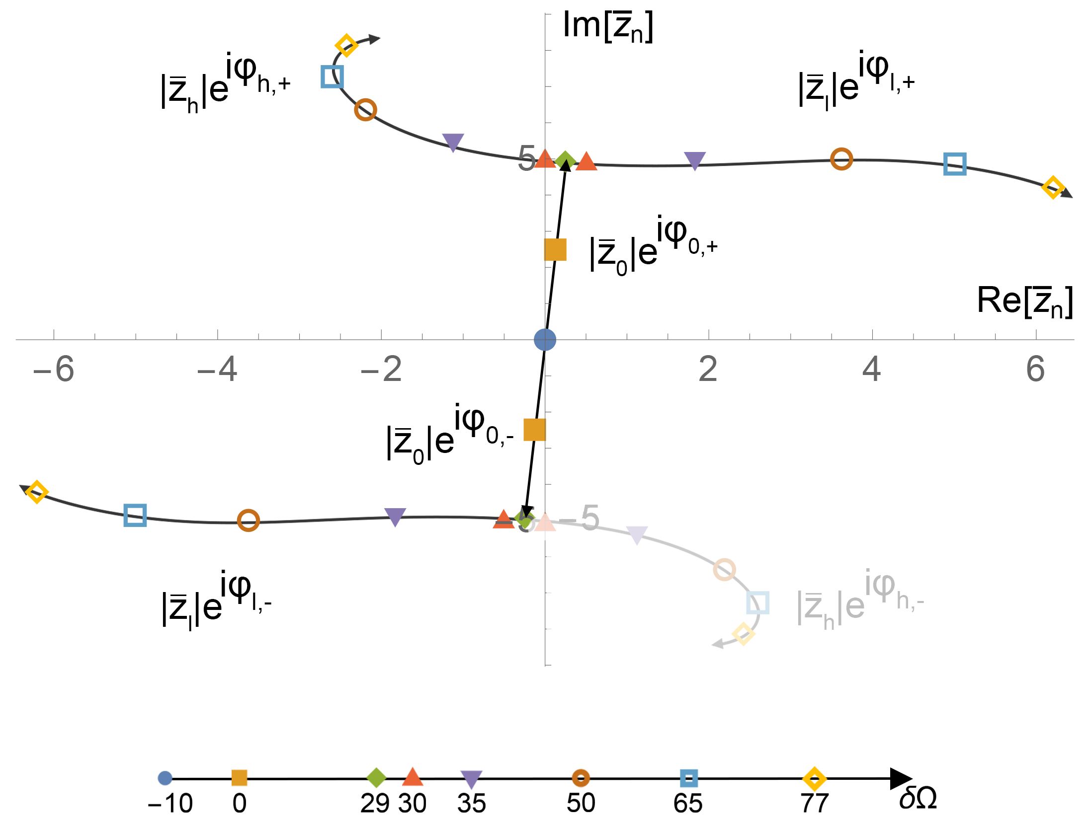
Figure 4: An example of the behavior of the system in the presence of a broken-symmetry solution corresponding to the parameters shown in Fig. 3 (a). Parameters: $g=1/5$, $\delta\Omega_{T,1}=\delta\Omega_{T,2}=10$. The stable solutions for the two amplitudes at different values of the detuning are shown. Before the bifurcation, we have the symmetric solutions $|\bar{z}_{0}|$, which are placed on a diagonal through the origin: the two modes can have either the same phase or a phase shift by $\pi$ (see text). After the bifurcation, we obtained different stable paired solutions. For example the solution $z_{1}=|\bar{z}_{h}|e^{i\varphi_{h,+}}$ in quadrant II can be paired either with $z_{2}=|\bar{z}_{l}|e^{i\varphi_{h,+}}$ in quadrant I or with $z_{2}=|\bar{z}_{l}|e^{i\varphi_{h,-}}$ in quadrant III.

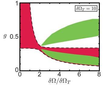
Figure 5: Phase diagram for the symmetric resonators with equal resonant frequency and drive strength $\delta\Omega_{T}=10$. The symmetric solutions $|\bar{z}_{1}|=|\bar{z}_{2}|$ are stable (unstable) in the white (red) region. The broken symmetry solutions are stable in the green region.

In Fig. 5, we show the complete phase diagram. The white areas represent regions where symmetric solutions are dynamically stable. In contrast, red areas indicate regions of dynamic instability for these solutions. Green areas denote the existence and dynamic stability of broken-symmetry solutions. When green overlaps with red, the broken-symmetry solution is the only stable configuration. Conversely, where green overlaps with white, both symmetric and broken-symmetry solutions remain dynamically stable.

We found the stability regions for the broken-symmetry solutions numerically, whereas the symmetric solutions are obtained from analytical formulas discussed in the previous section. A similar phase diagram occurs if we vary the symmetric drive strength $\delta\Omega_{T,1}=\delta\Omega_{T,2}$ where the critical coupling at $g_{c}\approx 1/3$ remains unchanged.

Given the parametric form of the driving and of the coupling, one must not forget that solutions where at least one oscillator is at rest, $z_{1}=0$ or $z_{2}=0$, are always possible.

VII Summary

In conclusion, we have studied the dynamics of a system of two parametrically driven nonlinear oscillators coupled by a nonlinear interaction. Several cases have been identified for which analytic solutions for the stationary state are available, while dynamic stability can be numerically assessed. As a most interesting result, in the symmetric case where the oscillators have equal parameters and are subject to equal driving forces, stationary solutions that spontaneously break the symmetry are found, leading to intriguing multistability phenomena. The natural next step will be to investigate the fluctuation properties around the critical points for this multistability phenomenon and the dependence of the switching rate between different solutions on the distance from the critical point.

Another interesting perspective is given by the recent advances in the field of superconducting circuits [36], where these types of nonlinear oscillators can be implemented by using various Josephson junction-based technologies [1, 37]. In this framework, the system can reach a regime where quantum effects become relevant. The pitchfork bifurcation leading to symmetry breaking in the steady-state solutions can eventually be described by a spontaneous symmetry-breaking dissipative phase transition in the quantum regime where the switching process is triggered by quantum fluctuations. Our findings can thus provide an interesting starting point to explore new types of dissipative phase transition in which the broken symmetry phase is multistable [38, 39, 40, 41, 42, 43].

Appendix A The model Hamiltonian

In this appendix we derive Eqs. (1),(2). We start from the model Hamiltonian that describes two nonlinear resonators of frequency $\omega_{n}$ with $n=1,2$ and Kerr-Duffing parameter $\kappa_{n}$ on which one applies one or two parametric external drives at frequency $2\omega_{d}$ and of strength $\mu_{n}$.

The two modes also have a dispersive interaction of coupling strength $\lambda$. The Hamiltonian of the system reads

$$H=\sum_{n=1}^{2}H_{n}+\frac{\lambda}{2}q_{1}^{2}q_{2}^{2}$$ (30)

with

$$H_{n}=\frac{p_{n}^{2}}{2}+\left(\frac{\omega_{n}^{2}}{2}+\mu_{n}\cos\left(2\omega_{d}t\right)\right)q_{n}^{2}+\frac{\kappa_{n}}{4}q_{n}^{4}$$ (31)

with $q_{n}$ and $p_{n}$ the conjugated variables (i.e. position and momentum) of the two modes. The dynamics equations are given by

$$\frac{\partial q_{n}}{\partial t}=\frac{\partial H}{\partial p_{n}}\,,\qquad\frac{\partial p_{n}}{\partial t}=-\frac{\partial H}{\partial q_{n}}-2\Gamma_{n}\frac{\partial q_{n}}{\partial t}$$ (32)

in which we added a damping force acting on both resonators with damping coefficient $\Gamma_{n}$. We apply a canonical transformation

$$q_{n}(t)=\frac{1}{2}u_{n}(t)e^{i\omega_{d}t}+\mbox{c.c.}\,,\,\,\,p_{n}(t)=\frac{i\omega_{d}}{2}u_{n}(t)e^{i\omega_{d}t}-\mbox{c.c.}$$ (33)

where c.c. means complex conjugate. Here $u_{n}(t)=X_{n}(t)-iY_{n}(t)$ is the complex amplitude whose components represent the two quadratures of the driven motion in the rotating frame, with $X_{n}(t)$ the component in phase with the drive and $Y_{n}(t)$ the component out of phase, namely $q_{n}(t)=X_{n}(t)\cos(\omega_{d}t)+Y_{n}(t)\sin(\omega_{d}t)$.

Using the rotating wave approximation (RWA) with $\omega_{d}\gg|\omega_{d}-\omega_{n}|$, the fast oscillating components of the motion in the rotating frame can be neglected, and the following time-independent equation for the quadratures is obtained

$$\frac{\partial X_{n}}{\partial t}=\frac{\partial H_{\mathrm{RWA}}}{\partial Y_{n}}-\Gamma_{n}X_{n}\,,\quad\frac{\partial Y_{n}}{\partial t}=-\frac{\partial H_{\mathrm{RWA}}}{\partial X_{n}}-\Gamma_{n}Y_{n}\,.$$ (34)

The conservative dynamic is described by the effective Hamiltonian $H_{\mathrm{RWA}}$. Before giving the explicit form of $H_{\mathrm{RWA}}$, it is useful to scale the quadrature according to the following way

$$X_{n}=\sqrt{\frac{8\omega_{d}\Gamma_{n}}{3\kappa_{n}}}Q_{n}\,,\qquad Y_{n}=\sqrt{\frac{8\omega_{d}\Gamma_{n}}{3\kappa_{n}}}P_{n}$$ (35)

where $Q_{n},P_{n}$ are dimensionless. Then, the effective Hamiltonian $H_{\mathrm{RWA}}$ can be cast as

$$\tilde{H}_{\mathrm{RWA}}=\frac{3\sqrt{\gamma_{1}\gamma_{2}}}{8\omega_{d}\Gamma_{1}\Gamma_{2}}H_{\mathrm{RWA}}=\alpha\,\tilde{H}_{1}+\frac{1}{\alpha}\,\tilde{H}_{2}+g\,\tilde{H}_{int}$$ (36)

with the parameters

$$g=\frac{\lambda}{3\sqrt{\kappa_{1}\kappa_{2}}}\,,\quad\alpha=\frac{\Gamma_{1}}{\Gamma_{2}}\sqrt{\frac{\kappa_{2}}{\kappa_{1}}}$$ (37)

$g$ represents the scaled coupling strength for the interaction, whereas $\alpha$ is the asymmetry parameter. The dimensionless Hamiltonians are given by

$$\tilde{H}_{n} =\frac{1}{4}{\left(Q_{n}^{2}+P_{n}^{2}\right)}^{2}-\frac{\delta\Omega_{n}}{2}{\left(Q_{n}^{2}+P_{n}^{2}\right)}$$

$$+\frac{\delta\Omega_{T,n}}{2}{\left(Q_{n}^{2}-P_{n}^{2}\right)}$$ (38)

$$\tilde{H}_{int} ={\left(Q_{1}^{2}+P_{1}^{2}\right)}{\left(Q_{2}^{2}+P_{2}^{2}\right)}+\frac{1}{2}{\left(Q_{1}^{2}-P_{1}^{2}\right)}{\left(Q_{2}^{2}-P_{2}^{2}\right)}$$

$$+2Q_{1}Q_{2}P_{1}P_{2}$$ (39)

and the scaled parameters are

$$\delta\Omega_{n}=\frac{\omega_{d}-\omega_{n}}{\Gamma_{n}}\,,\qquad\delta\Omega_{T,n}=\frac{\mu_{n}}{2\omega_{d}\Gamma_{n}}$$ (40)

with $\delta\Omega_{n}$ representing the scaled detuning for the resonator $n$ and $\delta\Omega_{T,n}$ is associated with the frequency threshold for the oscillatory motion of the resonator $n$ at frequency $\omega_{d}$ in the limit of vanishing damping and no interaction $g=0$. Setting $z_{n}=Q_{n}-iP_{n}$ the dynamical equations read

$$\frac{1}{\Gamma_{1}}\frac{\partial z_{1}}{\partial t} =\left(-i\delta\Omega_{1}+i{|z_{1}|}^{2}-1\right)z_{1}+i\delta\Omega_{T,1}z_{1}^{*}$$

$$+i\frac{g}{\alpha}\left(2{|z_{2}|}^{2}z_{1}+z_{2}^{2}z_{1}^{*}\right)$$ (41)

$$\frac{1}{\Gamma_{2}}\frac{\partial z_{2}}{\partial t} =\left(-i\delta\Omega_{2}+i{|z_{2}|}^{2}-1\right)z_{2}+i\delta\Omega_{T,2}z_{2}^{*}$$

$$+i\alpha g\left(2{|z_{1}|}^{2}z_{2}+z_{2}^{1}z_{2}^{*}\right)\,.$$ (42)

In the main text, we assumed that the resonators are almost equal and the asymmetry factor is $\alpha\approx 1$. More precisely, we consider $\Gamma_{1}\approx\Gamma_{2}$ which implies $\kappa_{1}\approx\kappa_{2}$ for $\alpha=1$. This is valid for $\Gamma_{n}\gg|\Gamma_{1}-\Gamma_{2}|$ and $\kappa_{n}\gg|\kappa_{1}-\kappa_{2}|$, i.e. the difference between the parameters are small corrections. Therefore, to simplify the notation, we set $\Gamma_{1}\approx\Gamma_{2}=\Gamma$ and $\kappa_{1}\approx\kappa_{2}=\kappa$. By scaling the time as $\tau=\Gamma t$ we obtain Eqs. (1),(2).

Appendix B The noninteracting case $g=0$ and the steady-state trivial solution $\bar{z}_{1}=\bar{z}_{2}=0$

In this appendix, we recall the solutions for the noninteracting case $g=0$ and analyze the behavior of the trivial solutions $\bar{z}_{1}=\bar{z}_{2}=0$.
For the uncoupled case $g=0$, we have a single parametrically driven nonlinear resonator. Within the RWA and in the limit of vanishing damping, the equation for the stationary solution for the first resonator reads

$$0=\left({|z_{1}|}^{2}-\delta\Omega_{1}\right)z_{1}+\left(\delta\Omega_{T,1}\right)z_{1}^{*}$$ (43)

and the non-trivial solutions for $z_{1}$ are simply

$$\bar{z}^{(0)}_{1,+}=\pm i\sqrt{\delta\Omega_{1}+\delta\Omega_{T,1}}\,,\,\,\,\,\bar{z}^{(0)}_{1,-}=\pm\sqrt{\delta\Omega_{1}-\delta\Omega_{T,1}}\,,$$ (44)

The solution $\bar{z}^{(0)}_{1,+}$ corresponds to the the resonator state when it starts to oscillate at frequency $\omega_{d}$ above the detuning threshold $\delta\Omega>-\delta\Omega_{T,1}$ and it is completely out of phase with respect to the drive. By analyzing the dynamics of the harmonic fluctuations around the stationary point, this solution is always dynamically stable above the threshold. The solution $\bar{z}^{(0)}_{1,-}$ appears above the detuning threshold $\delta\Omega>\delta\Omega_{T,1}$ and it is in phase respect to the drive: This solution is always dynamically unstable above the corresponding threshold. The trivial solution $\bar{z}^{(0)}_{1}=0$ is unstable in the detuning range $|\delta\Omega|<\delta\Omega_{T,1}$.

The effect of finite damping $\Gamma\neq 0$ is a shift of the detuning threshold $\delta\Omega_{T,1}\rightarrow{(\delta\Omega_{T,1}^{2}-1)}^{1/2}$, which reads, using the bare parameters, as the change from $\mu_{1}/(2\omega_{d})\rightarrow{[{(\mu_{1}/(2\omega_{d}))}^{2}-\Gamma^{2}]}^{1/2}$.

When we switch on the interaction, we discuss the stationary pair solutions. In this case, the trivial solutions $\left(\bar{z}_{1}=0,\bar{z}_{2}=0\right)$ is still a stationary solution which remains unstable for $|\delta\Omega_{i}|<\delta\Omega_{T,i}$ as for the case $g=0$ since the equations for the fluctuations around the stationary points are decoupled and uncorrelated as for the noninteracting case $g=0$.

Appendix C Solutions with $\bar{z}_{2}=0$

In this appendix, we discuss the behavior of the solutions of the type $(\bar{z}_{1}\neq 0,\bar{z}_{2}=0)$, namely when one of the two resonators does not oscillate.
The equations for the fluctuations of the two resonators are decoupled, and in particular, the dynamical equations for the fluctuations of the resonator with $\bar{z}_{1}\neq 0$ remain unchanged respect to the noninteracting case $g=0$.

However, the two resonators are correlated as the finite value of the amplitude of the first resonator $\bar{z}_{1}$ affects the fluctuations $\delta z_{2}$ of the second one with $\bar{z}_{2}=0$. Therefore, the stability range can differ from that of the noninteracting case. As a consequence, the stationary pair solution, which is stable for the case $g=0$ $\left(\bar{z}_{1,+}=\pm i\sqrt{\delta\Omega+\delta\Omega_{T,1}},\bar{z}_{2}=0\right)$ can become unstable. For example, in the regime $\omega_{1}=\omega_{2}$, $\delta\Omega_{T,2}<g\delta\Omega_{T,1}$ and $g<1/2$, the zero amplitude solution for the second resonator $\bar{z}_{2}=0$ becomes unstable in the detuning range $\delta\Omega_{T,2}<\delta\Omega<\left(2g\delta\Omega_{T,1}-\delta\Omega_{T,2}\right)/(1-2g)$, well beyond the range of the noninteracting case $|\delta\Omega|<\delta\Omega_{T,2}$.

Appendix D Analytic solutions for $\delta\Omega_{T,1}>0$ and $\delta\Omega_{T,2}=0$

In this appendix, we analyze in more detail the pair solution $\bar{z}_{1}\neq 0$ $\bar{z}_{2}\neq 0$ when only one resonator is parametrically driven, e.g. $\delta\Omega_{T,1}>0$ and $\delta\Omega_{T,2}=0$. Simple analytical solutions are possible in this case. To simplify the notation we consider degenerate resonators with $\omega_{1}\approx\omega_{2}$, namely $|\omega_{1}-\omega_{2}|\ll\Gamma$. If we consider one of the two equations for vanishing parametric drive for the second resonator, we have a simple equation

$$0=\left({|z_{1}|}^{2}-\delta\Omega+2g{|z_{1}|}^{2}\right)z_{2}+\left(z_{1}^{2}\right)z_{2}^{*}$$ (45)

Comparing Eq. (45) with Eq. (43) we see that the dispersive interaction has two effects: (i) the amplitude of the first resonator $z_{1}$ acts as a parametric drive on the second resonator, (ii) the amplitude of the first resonator $z_{1}$ leads to a dispersive frequency shift of the frequency of the second resonator. This equation can be solved for $z_{2}$ as function of $z_{1}$

$$z_{2,+}(z_{1}) =i\sqrt{\delta\Omega-g{|z_{1}|}^{2}}e^{i\theta_{1}}\,,\,\,\mbox{for}\,\,\delta\Omega-g{|z_{1}|}^{2}>0$$ (46)

$$z_{2,-}(z_{1}) =\sqrt{\delta\Omega-3g{|z_{1}|}^{2}}e^{i\theta_{1}}\,,\,\,\mbox{for}\,\,\delta\Omega-3g{|z_{1}|}^{2}>0$$ (47)

with $z_{1}=|z_{1}|e^{i\theta_{1}}$. As a consequence, these two solutions correspond to the two branches of the single parametrically driven Duffing that we have discussed above, with the difference that these two branches do not start symmetrically with respect to zero detuning, but they are centered at finite detuning $2g{|z_{1}|}^{2}$. Then we insert the two solutions $z_{2,\pm}(z_{1})$ in the equation $F_{1}\left(z_{1},z_{2,\pm}(z_{1})\right)=0$, in the limit of vanishing damping, such that we obtain a close equation for $z_{1}$. According to the value of coupling strength $g$ one obtains a zoo of different pair solutions. The non-trivial analytic solutions are reported in the table 1.

Notice that some solutions exist only in a given range of the coupling strength $g$. In particular different solutions appear in the range $0<g<1/3$, $1/3<g<1$ and $g>1$. The second column of the table 1 gives the frequency detuning threshold for the validity of the solutions, whereas the third column refers to the frequency detuning at which a discontinuity occurs. When the detuning threshold coincides with the detuning of the discontinuity, one of the two solutions is characterized by a jump from zero to the state of finite amplitude solution. When the detuning threshold is determined by the parametric drive $\delta\Omega_{T,1}$, the solutions are continuous and only the first derivative of the solution with respect to the detuning has a discontinuity.

The solutions in table 1 are possible solutions. However, as second step, we analyze the dynamical stability of these stationary solutions. In general, the region of stability does not coincide with the detuning threshold at which the stationary solution appears, and we must hence compute the stability ranges numerically.

In Fig. 1, we reported an example to illustrate the typical behavior of the system with the discontinuity in the first derivative of $\bar{z}_{1}$ as a function of detuning and the parametric-like threshold for $\bar{z}_{2}$.

Condition	Range	Discontinuity	$\bar{z}_{1}$	$\bar{z}_{2}$
$g<1$	$\delta\Omega>-\delta\Omega_{T,1}$	$\delta\Omega_{c,1}=\frac{g}{1-g}\delta\Omega_{T,1}$	$\pm i\sqrt{\delta\Omega+\delta\Omega_{T,1}-\theta\left(\delta\Omega-\delta\Omega_{c,1}\right)\frac{g}{1+g}\left(\delta\Omega-\delta\Omega_{c,1}\right)}$	$\mp\sqrt{\delta\Omega-g{|\bar{z}_{1}|}^{2}}$
$g<1$	$\delta\Omega>\delta\Omega_{c,2}$	$\delta\Omega_{c,2}=\frac{1}{1-g}\delta\Omega_{T,1}$	$\pm\sqrt{\frac{1}{1+g}\left(\delta\Omega-\delta\Omega_{c,2}\right)}$	$\pm i\sqrt{\delta\Omega-g{|\bar{z}_{1}|}^{2}}$
$1<g$	$\delta\Omega>\delta\Omega_{c,1}^{*}$	$\delta\Omega_{c,1}^{*}=\frac{1}{g-1}\delta\Omega_{T,1}$	$\pm i\sqrt{\frac{1}{1+g}\left(\delta\Omega-\delta\Omega_{c,1}^{*}\right)}$	$\mp\sqrt{\delta\Omega-g{|\bar{z}_{1}|}^{2}}$
$1<g$	$\delta\Omega>\delta\Omega_{T,1}$	$\delta\Omega_{c,2}^{*}=\frac{g}{g-1}\delta\Omega_{T,1}$	$\pm\sqrt{\delta\Omega-\delta\Omega_{T,1}-\theta\left(\delta\Omega-\delta\Omega_{c,2}^{*}\right)\frac{g}{1+g}\left(\delta\Omega-\delta\Omega_{c,2}^{*}\right)}$	$\pm i\sqrt{\delta\Omega-g{|\bar{z}_{1}|}^{2}}$
$g<\frac{1}{3}$	$\delta\Omega>-\delta\Omega_{T,1}$	$\delta\Omega_{c,3}=\frac{3g}{1-3g}\delta\Omega_{T,1}$	$\pm i\sqrt{\delta\Omega+\delta\Omega_{T,1}-\theta\left(\delta\Omega-\delta\Omega_{c,3}\right)\frac{3g}{1+3g}\left(\delta\Omega-\delta\Omega_{c,3}\right)}$	$\pm i\sqrt{\delta\Omega-3g{|\bar{z}_{1}|}^{2}}$
$g<\frac{1}{3}$	$\delta\Omega>\delta\Omega_{c,4}$	$\delta\Omega_{c,4}=\frac{1}{1-3g}\delta\Omega_{T,1}$	$\pm\sqrt{\frac{1}{1+3g}\left(\delta\Omega-\delta\Omega_{c,4}\right)}$	$\pm\sqrt{\delta\Omega-3g{|\bar{z}_{1}|}^{2}}$
$\frac{1}{3}<g$	$\delta\Omega>\delta\Omega_{c,3}^{*}$	$\delta\Omega_{c,3}^{*}=\frac{1}{3g-1}\delta\Omega_{T,1}$	$\pm i\sqrt{\frac{1}{1+3g}\left(\delta\Omega-\delta\Omega_{c,3}^{*}\right)}$	$\pm i\sqrt{\delta\Omega-3g{|\bar{z}_{1}|}^{2}}$
$\frac{1}{3}<g$	$\delta\Omega>\delta\Omega_{T,1}$	$\delta\Omega_{c,4}^{*}=\frac{3g}{3g-1}\delta\Omega_{T,1}$	$\pm\sqrt{\delta\Omega-\delta\Omega_{T,1}-\theta\left(\delta\Omega-\delta\Omega_{c,4}^{*}\right)\frac{3g}{1+3g}\left(\delta\Omega-\delta\Omega_{c,4}^{*}\right)}$	$\pm\sqrt{\delta\Omega-3g{|\bar{z}_{1}|}^{2}}$

Table 1: Non-trivial analytic solutions of the stationary state for a single driven mode, for the symmetric case, and in the limit
small damping.

References

- Dykman [2012] M. Dykman, Fluctuating nonlinear oscillators: from nanomechanics to quantum superconducting circuits (Oxford University Press, 2012).
- Cleland [2003] A. Cleland, Foundation of nanomechanics: from solid-state theory to device applications (Springer Berlin, Heidelberg, 2003).
- Schmid et al. [2016] S. Schmid, L. Villanueva, and M. Roukes, Fundamental of nanomechanical resonators (Springer Cham, 2016).
- Cleland and Roukes [2002] A. Cleland and M. Roukes, J. App. Phys. 92, 2758 (2002).
- Lifshitz and Cross [2008a] R. Lifshitz and M. Cross, Nonlinear dynamics of nanomechanical and micromechanical resonators (H.G. Schuster, Wiley Meinheim Press, 2008) Chap. 1 in ”Review of nonlinear dynamics and complexity”.
- Poot and van der Zant [2012] M. Poot and H. van der Zant, Phys. Rep. 511, 273 (2012).
- Rhoads et al. [2010] J. Rhoads, S. Shaw, and K. L. Turner, J. Dyn. Sys. Meas. Control. 132, 034001 (2010).
- Lifshitz and Cross [2008b] R. Lifshitz and M. C. Cross, “Nonlinear dynamics of nanomechanical and micromechanical resonators,” in Reviews of Nonlinear Dynamics and Complexity (John Wiley and Sons, Ltd, 2008) Chap. 1, pp. 1–52.
- Güttinger et al. [2017] J. Güttinger, A. Noury, P. Weber, A. M. Eriksson, C. Lagoin, J. Moser, C. Eichler, A. Wallraff, A. Isacsson, and A. Bachtold, Nature Nanotechnology 12, nnano.2017.86 (2017).
- Chen et al. [2017] C. Chen, D. H. Zanette, D. A. Czaplewski, S. Shaw, and D. Lopez, Nature Communications 8, ncomms15523 (2017).
- Bachtold et al. [2022] A. Bachtold, J. Moser, and M. I. Dykman, Rev. Mod. Phys. 94, 045005 (2022).
- Lugiato [1983] L. A. Lugiato, Contemporary Physics 24, 333 (1983).
- Butcher and Cotter [2008] P. N. Butcher and D. Cotter, The elements of nonlinear optics, Cambridge Studies in Modern Optics (Cambridge University Press, 2008).
- Boyd [2008] R. W. Boyd, Nonlinear Optics (Academic Press, 2008).
- Walls and Milburn [2006] D. F. Walls and G. Milburn, Quantum Optics (Springer Verlag, Berlin, 2006).
- Drummond and Hillery [2014] P. D. Drummond and M. Hillery, The quantum theory of nonlinear optics (Cambridge University Press, 2014).
- Nayfeh and Mook [1979] A. Nayfeh and D. Mook, Nonlinear oscillationss (Wiley-VCH Press, 1979).
- Westra et al. [2010] H. J. R. Westra, M. Poot, H. S. J. van der Zant, and W. J. Venstra, Phys. Rev. Lett. 105, 117205 (2010).
- Lulla et al. [2012] K. J. Lulla, R. B. Cousins, M. J. Venkatesan, A. andPatton, A. D. Armour, C. J. Mellor, and J. R. Owers-Bradley, New J. Phys. 14, 113040 (2012).
- Matheny et al. [2013] M. H. Matheny, L. G. Villanueva, R. B. Karabalin, J. E. Sader, and M. L. Roukes, Nano Lett. 13, 1622 (2013).
- Vinante [2014] A. Vinante, Physical Review B 90, 024308 (2014).
- Mangussi and Zanette [2016] F. Mangussi and D. H. Zanette, PLOS ONE 11, e0162365 (2016).
- Cadeddu et al. [2016] D. Cadeddu, F. R. Braakman, G. Tütüncüoglu, F. Matteini, D. Rüffer, A. Fontcuberta i Morral, and M. Poggio, Nano Lett. 16, 926 (2016).
- Dong et al. [2018] X. Dong, M. Dykman, and H. Chan, Nat. Comm. 9, 3241 (2018).
- Mathew et al. [2018] J. P. Mathew, A. Bhushan, and M. M. Deshmukh, Solid State Communications 282, 17 (2018).
- Gajo et al. [2020] K. Gajo, G. Rastelli, and E. M. Weig, Physical Review B 101, 075420 (2020).
- Valagiannopoulos et al. [2021] C. Valagiannopoulos, A. Sarsen, and A. Alu, IEEE Transactions on Antennas and Propagation 69, 7720 (2021).
- Carusotto and Ciuti [2013] I. Carusotto and C. Ciuti, Rev. Mod. Phys. 85, 299 (2013).
- Abbarchi et al. [2013] M. Abbarchi, A. Amo, V. Sala, D. Solnyshkov, H. Flayac, L. Ferrier, I. Sagnes, E. Galopin, A. Lemaître, G. Malpuech, et al., Nature Physics 9, 275 (2013).
- Wouters and Carusotto [2007] M. Wouters and I. Carusotto, Phys. Rev. B 75, 075332 (2007).
- Sarchi et al. [2008] D. Sarchi, I. Carusotto, M. Wouters, and V. Savona, Phys. Rev. B 77 (2008), 10.1103/PhysRevB.77.125324.
- Cross and Hohenberg [1993] M. C. Cross and P. C. Hohenberg, Rev. Mod. Phys. 65, 851 (1993).
- Fontaine et al. [2022] Q. Fontaine, D. Squizzato, F. Baboux, I. Amelio, A. Lemaître, M. Morassi, I. Sagnes, L. Le Gratiet, A. Harouri, M. Wouters, et al., Nature 608, 687 (2022).
- Claude et al. [2023] F. Claude, M. J. Jacquet, M. Wouters, E. Giacobino, Q. Glorieux, I. Carusotto, and A. Bramati, preprint arXiv:2310.11903 (2023).
- Zamora et al. [2017] A. Zamora, L. M. Sieberer, K. Dunnett, S. Diehl, and M. H. Szymańska, Phys. Rev. X 7, 041006 (2017).
- Blais et al. [2021] A. Blais, A. L. Grimsmo, S. M. Girvin, and A. Wallraff, Rev. Mod. Phys. 93, 025005 (2021).
- Hu et al. [2011] Y. Hu, G.-Q. Ge, S. Chen, X.-F. Yang, and Y.-L. Chen, Phys. Rev. A 84, 012329 (2011).
- Savona [2017] V. Savona, Phys. Rev. A 96, 033826 (2017).
- Nagy and Savona [2018] A. Nagy and V. Savona, Phys. Rev. A 97, 052129 (2018).
- Seibold et al. [2020] K. Seibold, R. Rota, and V. Savona, Phys. Rev. A 101, 033839 (2020).
- Fink et al. [2017] J. M. Fink, A. Dombi, A. Vukics, A. Wallraff, and P. Domokos, Phys. Rev. X 7, 011012 (2017).
- Minganti et al. [2023] F. Minganti, V. Savona, and A. Biella, Quantum 7, 1170 (2023).
- Beaulieu et al. [2023] G. Beaulieu, F. Minganti, S. Frasca, V. Savona, S. Felicetti, R. D. Candia, and P. Scarlino, “Observation of first- and second-order dissipative phase transitions in a two-photon driven kerr resonator,” (2023), arXiv:2310.13636 [quant-ph] .