High harmonic generation from electrons moving on topological spin textures

Abstract

High harmonic generation (HHG) is a striking phenomenon, which reflects the ultrafast dynamics of electrons. Recently, it has been demonstrated that HHG can be used to reconstruct not only the energy band structure but also the geometric structure characterized by the Berry curvature. Here, we numerically investigate HHG arising from electrons coupled with a topological spin texture in a spin scalar chiral state where time reversal symmetry is broken. In this system, a sign change in scalar chirality alters the sign of the Berry curvature while keeping the energy band structure unchanged, allowing us to discuss purely geometrical effects on HHG. Notably, we found that, when the optical frequency is significantly lower than the energy gap, the sign of scalar chirality largely affects the longitudinal response parallel to the optical field rather than the transverse response. Our analysis suggests that this can be attributed to interband currents induced by the recombination of electron–hole pairs whose real-space trajectories are modulated by the anomalous velocity term.

I Introduction

With the advancement of laser technology, ultrafast phenomena in the sub-femtosecond and attosecond domains are being actively researched [1, 2, 3, 4, 5, 6, 7, 8, 9, 10, 11, 12, 13, 14]. High harmonic generation (HHG) and high-order sideband generation (HSG) are representative examples, and recent research has progressed in solids such as semiconductors [15, 16, 17, 18, 19, 20, 21, 22, 23, 24, 25, 26, 27, 28, 29, 30, 31, 32, 33, 34, 35, 36, 37], strongly correlated electron systems [38, 39, 40, 41, 42, 43, 44, 45, 46, 47, 48, 49, 50, 51, 52, 53, 54, 55, 56, 57, 58, 59], and magnetic materials [60, 61, 62, 63, 64, 65, 66, 67, 68, 69]. In HHG and HSG, high-order harmonics are literally generated, and the details of their spectra and chirping have been well captured by the three-step model [70, 71, 72, 73, 74]. According to this model, the elementary processes of HHG, for example, consist of (i) ionization of electrons to the vacuum or excitation to the conduction bands, (ii) acceleration, and (iii) recombination of the electrons or the electron–hole pairs. Therefore, the electronic structure is embedded in the high harmonic spectrum, and using this property, all-optical reconstruction of energy bands through HHG and HSG has been proposed and experimentally demonstrated [75, 76, 77, 78, 79, 74].

Recently, it has become increasingly clear that HHG can be used to extract not only the energy band structure but also the geometric structure of electrons, characterized by the Berry curvature or the Berry phase [80, 81, 82, 83, 84, 85, 86, 87, 88, 89, 90]. As is well known, the Berry curvature appears in systems where either spatial inversion symmetry or time reversal symmetry is broken. Hitherto, high harmonics dependent on the Berry curvature have been observed in systems with broken spatial inversion symmetry, for example, in a monolayer $\mathrm{MoS_{2}}$ [80] and the surface states of a topological insulator $\mathrm{Bi_{2}Te_{3}}$ [81]. Additionally, in a Weyl semimetal $\mathrm{WP_{2}}$ [82], the Berry curvature has been successfully reconstructed in reciprocal space. However, studies on the effects of geometric structures in HHG have been scarce for systems with broken time reversal symmetry.

Systems exhibiting nonzero Berry curvature due to broken time reversal symmetry include those with what are called topological spin textures. For example, in skyrmion crystals, interesting perturbative linear responses such as the topological Hall effect [91] and the magneto-optical effect [92, 93, 94, 95, 96] have been reported and discussed. However, nonperturbative nonlinear responses, such as HHG or HSG, are largely unexplored, even though the magnetic structure is expected to be embedded in the high harmonic spectrum through the dynamics of electrons coupled with topological spin textures.

A spin scalar chiral state can be considered as one of the simplest topological spin textures. It features a four-sublattice magnetic order [Figs. 1(a) and 1(b)], where the Chern number of each energy band takes on an integer value, leading to the emergence of the anomalous (topological) Hall effect [97, 98]. Hence, this state can be viewed as a skyrmion crystal state with the smallest magnetic unit cell. Last year, two groups experimentally reported that the scalar chiral state is realized in $\mathrm{CoTa_{3}S_{6}}$ and $\mathrm{CoNb_{3}S_{6}}$ [99, 100, 101], attracting significant interest. In this study, we numerically analyze HHG in the scalar chiral state. We found that the transverse response, as naively expected to reflect the Berry curvature, indeed appears. Furthermore, we discovered that the sign of the Berry curvature is reflected in the longitudinal response even in cases where it predominates over the transverse response. This finding differs from the effects of anomalous velocity in intraband currents that have been discussed previously. We argue that the anomalous velocity modulates the recombination conditions of electron–hole pairs, potentially changing the interband current spectrum, on the basis of an analysis of the real-space dynamics of electron–hole pairs.

The rest of this paper is organized as follows. In Sec. II, we introduce our model and methods, and in Sec. III, we present numerical results. Sec. III.1 provides an overview of the equilibrium properties, focusing particularly on its geometrical structure, and Sec. III.2 displays the high harmonic spectrum obtained from real-time evolution. The analysis of the real-space dynamics of electron–hole pairs is conducted in Sec. III.3. Sec. III.4 discusses HHG for parameters close to those for $\mathrm{CoTa_{3}S_{6}}$ and $\mathrm{CoNb_{3}S_{6}}$. Secs. IV and V are respectively devoted to the discussion and summary. Appendices A–C present results for near-resonant and circular polarization driving, as well as comparisons with the $120^{\mathrm{\circ}}$ Néel state, where the Berry curvature is absent.

II Model and method

To examine the dynamics of electrons coupled with spin textures, we consider the ferromagnetic Kondo lattice model (FKLM) on a two-dimensional triangular lattice. The Hamiltonian is defined by

$$\mathcal{H}=\sum_{ijs}h_{ij}c_{is}^{\dagger}c_{js}-J_{\mathrm{K}}\sum_{iss^{\prime}}\bm{S}_{i}\cdot\bm{\sigma}_{ss^{\prime}}c_{is}^{\dagger}c_{is^{\prime}},$$ (1)

where $c_{is}^{\dagger}$ is a creation operator of an electron at site $i$ with spin $s$, $\bm{\sigma}$ is a three-component vector of the Pauli matrices, and $\bm{S}_{i}$ is a classical vector describing a localized spin at site $i$. The transfer integral and the exchange interaction strength are denoted by $h_{ij}$ and $J_{\mathrm{K}}$, respectively. Considering that the electron dynamics induced by external fields occur on time scales of the order of subpicoseconds, we assume in this study that a magnetic order of $\{\bm{S}_{i}\}$ is not disturbed by electron motions; that is, each $\bm{S}_{i}$ is frozen during the real-time evolution of the electrons.

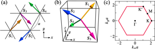
Figure 1: (a) Magnetic unit cell of the four-sublattice spin scalar chiral state and (b) configuration of the four localized spin vectors, adapted from Ref. [102]. (c) Magnetic Brillouin zone.

While the Hamiltonian in Eq. (1) is invariant under the global rotation of $\{\bm{S}_{i}\}$ and $\bm{\sigma}$, we explicitly define the four-sublattice scalar chiral state as

$$\bm{S}_{1}=\frac{(1,1,1)}{\sqrt{3}},\quad\bm{S}_{2}=\frac{(-1,-1,1)}{\sqrt{3}},$$

$$\bm{S}_{3}=\frac{(1,-1,-1)}{\sqrt{3}},\quad\bm{S}_{4}=\frac{(-1,1,-1)}{\sqrt{3}},$$ (2)

where $\bm{S}_{m}$ represents the localized spin of sublattice $m$ instead of site $i$ (see Fig. 1). For this choice of $\{\bm{S}_{m}\}$, the scalar chirality, defined by

$$\chi=\bm{S}_{1}\cdot(\bm{S}_{2}\times\bm{S}_{3})+\bm{S}_{4}\cdot(\bm{S}_{3}\times\bm{S}_{2}),$$ (3)

has a positive value of $\chi=8/(3\sqrt{3})\equiv\chi_{0}$. The sign of $\chi$ is changed by time reversal: $\bm{S}_{m}\mapsto-\bm{S}_{m}$ for all $m$; this operation is equivalent to $J_{\mathrm{K}}\mapsto-J_{\mathrm{K}}$ in the electron system, while the band structure remains unchanged, since the localized spins $\bm{S}_{m}$ are treated classically.

Assuming sublattice structure, we can express the Hamiltonian in reciprocal space as

$$\mathcal{H}=\sum_{\bm{k}}\sum_{ss^{\prime}}\sum_{mm^{\prime}}h_{sm,s^{\prime}m^{\prime}}(\bm{k})c_{\bm{k}sm}^{\dagger}c_{\bm{k}s^{\prime}m^{\prime}},$$ (4)

where $\bm{k}$ denotes momentum, and the indices $s$ and $m$ correspond respectively to the spin and sublattice degrees of freedom. In the four-sublattice scalar chiral state, each energy band is doubly degenerated in the whole magnetic Brillouin zone (BZ) [Fig. 1(c)], and $h(\bm{k})$ is an $8\times 8$ matrix that can be block diagonalized by the unitary transformation:

$$U^{\dagger}h(\bm{k})U=h_{+}(\bm{k})\oplus h_{-}(\bm{k}),$$ (5)

into two $4\times 4$ matrices $h_{+}$ and $h_{-}$. Adopting $\{\bm{S}_{m}\}$ in Eq. (2), we can choose the unitary matrix $U$ as

$$U =\text{(spin)}\otimes\text{(sublattice)}$$

$$=\frac{1}{\sqrt{2}}{\begin{bmatrix}-\mathrm{i}&0&0&0&\mathrm{i}&0&0&0\\ 0&-\mathrm{i}&0&0&0&\mathrm{i}&0&0\\ 0&0&-\mathrm{i}&0&0&0&\mathrm{i}&0\\ 0&0&0&-\mathrm{i}&0&0&0&\mathrm{i}\\ 0&0&0&1&0&0&0&1\\ 0&0&1&0&0&0&1&0\\ 0&1&0&0&0&1&0&0\\ 1&0&0&0&1&0&0&0\end{bmatrix}},$$ (6)

which diagonalizes another unitary matrix $V$ that commutes with $h(\bm{k})$. The latter unitary matrix,

$$V=\sigma_{y}\otimes{\begin{bmatrix}0&0&0&1\\ 0&0&1&0\\ 0&1&0&0\\ 1&0&0&0\end{bmatrix}},$$ (7)

represents a mirror reflection of electron spins with respect to the $zx$ plane and a permutation of sublattice spins: $\bm{S}_{1}\leftrightarrow\bm{S}_{4}$ and $\bm{S}_{2}\leftrightarrow\bm{S}_{3}$, and it is diagonalized as

$$U^{\dagger}VU=\operatorname{diag}(+1,+1,+1,+1,-1,-1,-1,-1).$$ (8)

The explicit form of $h_{\pm}$ is given by

$$h_{\pm}(\bm{k}) =-\frac{J_{\mathrm{K}}}{\sqrt{3}}\sigma_{z}\otimes\sigma_{0}\pm\frac{J_{\mathrm{K}}}{\sqrt{3}}(\sigma_{x}+\sigma_{y})\otimes\sigma_{y}$$

$$\quad-2h_{1}\cos(k_{x})\sigma_{0}\otimes\sigma_{x}$$

$$\quad-2h_{1}\cos\left(\frac{k_{x}+\sqrt{3}k_{y}}{2}\right)\sigma_{x}\otimes\sigma_{0}$$

$$\quad-2h_{1}\cos\left(\frac{k_{x}-\sqrt{3}k_{y}}{2}\right)\sigma_{x}\otimes\sigma_{x},$$ (9)

where $\sigma_{0}$ denotes the identity matrix. Here and throughout the paper, we consider only the transfer integral between the nearest neighbor sites, $h_{ij}=-h_{1}$. Given the above, we can write the Hamiltonian in Eq. (1) as

$$\mathcal{H}=\sum_{\bm{k}}\sum_{n=1}^{4}{\left[\varepsilon_{n}^{+}(\bm{k})a_{\bm{k}n}^{\dagger}a_{\bm{k}n}+\varepsilon_{n}^{-}(\bm{k})b_{\bm{k}n}^{\dagger}b_{\bm{k}n}\right]}$$ (10)

with $\varepsilon_{n}^{+}(\bm{k})=\varepsilon_{n}^{-}(\bm{k})\equiv\varepsilon_{n}(\bm{k})$. Here, $\varepsilon_{n}^{\pm}(\bm{k})$ is the $n$th eigen energy of $h_{\pm}(\bm{k})$, and $a_{\bm{k}n}^{\dagger}$ and $b_{\bm{k}n}^{\dagger}$ are creation operators of electrons associated with $c_{\bm{k}sm}^{\dagger}$ through an unitary transformation. The block diagonal form of $h(\bm{k})$ in Eq. (5) facilitates the efficient computation of real-time dynamics and enables the calculation of the Berry curvature $\bm{B}_{n}=(0,0,B_{n})$ through the following formula:

$$B_{n}(\bm{k})=\sum_{m(\neq n)}\frac{\langle\bm{k}n|v_{x}(\bm{k})|\bm{k}m\rangle\langle\bm{k}m|v_{y}(\bm{k})|\bm{k}n\rangle-\text{c.c.}}{[\varepsilon_{n}(\bm{k})-\varepsilon_{m}(\bm{k})]^{2}}$$ (11)

with $\bm{v}(\bm{k})=\partial_{\bm{k}}h_{+}(\bm{k})\ [=\partial_{\bm{k}}h_{-}(\bm{k})]$, where $|\bm{k}n\rangle$ is an energy eigenstate satisfying $h_{+}(\bm{k})|\bm{k}n\rangle=\varepsilon_{n}(\bm{k})|\bm{k}n\rangle$. Note that $B_{n}(\bm{k})$ remains unchanged even if we adopt the eigenstates of $h_{-}(\bm{k})$, and the Chern number of the doubly degenerated $n$th band is given by

$$\mathcal{C}_{n}=\int_{\text{BZ}}\frac{\mathrm{d}^{2}k}{2\pi}\,2B_{n}(\bm{k}),$$ (12)

where BZ stands for the magnetic BZ depicted in Fig. 1(c). We also introduce the linear optical conductivity [103],

$$\sigma_{\alpha\beta}(\omega) =\frac{\mathrm{i}T_{\alpha\beta}-\mathrm{i}\chi_{\alpha\beta}(\omega+\mathrm{i}\eta)}{\omega+\mathrm{i}\eta},$$ (13)

with $\eta$ being a positive infinitesimal, where

$$T_{\alpha\beta} =\int_{\text{BZ}}\frac{\mathrm{d}^{2}k}{(2\pi)^{2}}\operatorname*{Tr}[\rho_{\bm{k}}\partial_{k_{\alpha}}\partial_{k_{\beta}}h(\bm{k})],$$ (14)

$$\chi_{\alpha\beta}(z) =2\int_{\text{BZ}}\frac{\mathrm{d}^{2}k}{(2\pi)^{2}}\sum_{mn}\frac{f_{n}(\bm{k})-f_{m}(\bm{k})}{\varepsilon_{m}(\bm{k})-\varepsilon_{n}(\bm{k})-z}$$

$$\quad\times\langle\bm{k}n|v_{\alpha}(\bm{k})|\bm{k}m\rangle\langle\bm{k}m|v_{\beta}(\bm{k})|\bm{k}n\rangle.$$ (15)

Here, $\rho_{\bm{k},mn}=\langle c_{\bm{k}n}^{\dagger}c_{\bm{k}m}\rangle$ represents a one-body density matrix of electrons, $f_{n}(\bm{k})=\langle a_{\bm{k}n}^{\dagger}a_{\bm{k}n}\rangle=\langle b_{\bm{k}n}^{\dagger}b_{\bm{k}n}\rangle$ is the Fermi distribution function for the $n$th band, and $T_{\alpha\beta}$ in Eq. (14) is called a stress tensor. The prefactor $2$ in Eq. (15) counts the equal contribution from the eigenstates of $h_{-}$.

The real-time dynamics are governed by the von Neumann equation with a phenomenological relaxation term,

$$\frac{\mathrm{d}\rho_{\bm{k}}}{\mathrm{d}t}=-\mathrm{i}[h(\bm{k}),\rho_{\bm{k}}]-\varGamma(\rho_{\bm{k}}-\rho_{0,\bm{k}}),$$ (16)

with $t$ representing time. Here, $\rho_{0,\bm{k}}$ denotes the one-body density matrix in the ground state for a given $\bm{k}$, and $\varGamma$ represents the relaxation rate. We assume that the initial state is the ground state, that is, $\rho_{\bm{k}}(-\infty)=\rho_{0,\bm{k}}$. Given our focus on the dynamics of electrons driven by optical fields, we consider only the coupling between the electric field and the electrons. The vector potential $\bm{A}(t)$ is introduced through the Peierls substitution: $\bm{k}(t)=\bm{k}-\bm{A}(t)$, and the electric field $\bm{F}$ is determined by $\bm{F}(t)=-\partial_{t}\bm{A}(t)$. In this study, we apply a continuous wave described by the following vector potential:

$$A_{\alpha}(t) =-\frac{\bm{F}_{0,\alpha}}{\varOmega}\sin(\varOmega t-\phi_{\alpha})\times{\left\{\begin{array}[]{cl}\mathrm{e}^{-t^{2}/(2\tau^{2})}&(t<0)\\ 1&(t\geq 0)\end{array}\right.}$$ (19)

for $\alpha=x,y$, where $\bm{F}_{0}=(F_{0,x},F_{0,y})$, $\varOmega$, $\phi_{\alpha}$, and $\tau$ represent the electric field amplitude, frequency, phase, and ramp time, respectively. Linear polarization (LP) is characterized by

$$F_{0,x}=F_{0}\cos\psi,\quad F_{0,y}=F_{0}\sin\psi,\quad\phi_{x}=\phi_{y}=\phi,$$ (20)

where $\psi$ denotes the polarization angle measured from the $x$ axis [see also Fig. 1(a)]. On the other hand, left/right circular polarization (LCP/RCP) is described by

$$F_{0,x}=F_{0,y}=F_{0},\quad(\phi_{x},\phi_{y})={\left\{\begin{array}[]{cl}(-\pi/2,0)&(\text{LCP})\\ (+\pi/2,0)&(\text{RCP}).\end{array}\right.}$$ (23)

The electric current density $\bm{J}(t)$ is defined by

$$\bm{J}(t)=\frac{1}{N\mathcal{A}}\sum_{\bm{k}}\operatorname*{Tr}[\rho_{\bm{k}}\bm{v}(\bm{k})],$$ (24)

where $N$ stands for the number of $\bm{k}$-points. The area of the magnetic unit cell is denoted by $\mathcal{A}$, and in the presence of four-sublattice orders, $\mathcal{A}=2\sqrt{3}a^{2}$ with $a$ being the lattice constant. The intensity of electromagnetic radiation is proportional to

$$I(\omega)=I_{x}(\omega)+I_{y}(\omega),\quad I_{\alpha}(\omega)=\omega^{2}|J_{\alpha}(\omega)|^{2}$$ (25)

for $\alpha=x,y$, where $\bm{J}(\omega)$ is the Fourier transformation of $\bm{J}(t)$.

The von Neumann equation (16) is numerically solved using the fourth-order Runge–Kutta method with a time step of $\delta t=0.01\hbar/h_{1}$. The number of $\bm{k}$-points is set to $N=50^{2}$, for which we confirmed the convergence. In this paper, the nearest neighbor transfer integral $h_{1}$, the Dirac constant $\hbar$, the electric charge $e$, and the lattice constant $a$ are set to one. Energy, time, electric current density, and electric fields are expressed in units of $h_{1}$, $\hbar/h_{1}$, $eh_{1}/(\hbar a)$, and $h_{1}/(ea)$, respectively. For $h_{1}=1\ \mathrm{eV}$ and $a=1\ \mathrm{nm}$, these read $\hbar/h_{1}=0.66\ \mathrm{fs}$, $eh_{1}/(\hbar a)=2.4\ \mathrm{kA\,cm^{-1}}$, and $h_{1}/(ea)=10\ \mathrm{MV\,cm^{-1}}$.

III Results

In this section, we give an overview of the equilibrium properties of the four-sublattice scalar chiral state. Then, we show the numerical results of the HHG when linearly polarized light is applied, and discuss how geometrical effects manifest themselves. Hereafter, we focus mainly on cases where the Kondo coupling is $J_{\mathrm{K}}=3$, and the electron number density is $n_{\mathrm{e}}=0.5$ (half filling) . At half filling, the optical gap increases proportionally with $J_{\mathrm{K}}$, which enables numerical analysis at optical frequencies that are sufficiently small relative to the gap, suppressing the excited electron density in the conduction bands. Additionally, despite the absence of the dc Hall effect at $n_{\mathrm{e}}=0.5$, optical transverse responses due to the nonzero Berry curvature can be observed, as shown in the following sections.

III.1 Equilibrium properties

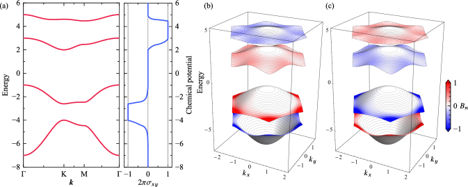
Figure 2: (a) Energy band structure $\varepsilon_{n}(\bm{k})$ (left panel), and the chemical potential dependence of dc Hall conductivity $2\pi\sigma_{xy}(0)$ at zero temperature (right panel), in the four-sublattice scalar chiral state. The conductivity is calculated using Eqs. (13)–(15) with $\eta=0.01$. (b), (c) Berry curvature $B_{n}(\bm{k})$ plotted on the energy-band surfaces, for (b) $\chi=+\chi_{0}$ and (c) $\chi=-\chi_{0}$.

Figure 2(a) displays the energy band structure $\varepsilon_{n}(\bm{k})$ in the magnetic BZ alongside the dc Hall conductivity as a function of the chemical potential. We observe four doubly degenerated bands in the magnetic BZ. The dc Hall conductivity $\sigma_{xy}(\omega=0)$ exhibits a quantized value of $\pm e^{2}/(2\pi\hbar)$ when the electrons are at quarter or three quarter filling, as initially pointed out in Refs. [97, 98]. Since time reversal symmetry is broken while spatial inversion symmetry is preserved, the Berry curvature satisfying $\bm{B}_{n}(-\bm{k})=\bm{B}_{n}(\bm{k})$ can appear in the scalar chiral state. In Figs. 2(b) and 2(c), we present the Berry curvature $B_{n}(\bm{k})$ on the energy-band surfaces for $\chi=+\chi_{0}$ and $\chi=-\chi_{0}$. For the lower two doubly degenerated bands, the Berry curvature takes on large values at and in the vicinity of the K point, while for the upper two bands, the Berry curvature appears more dispersed throughout the BZ. Notably, the sign of the Berry curvature is reversed by changing the sign of $\chi$ without affecting the energy bands $\varepsilon_{n}(\bm{k})$. The Chern number defined in Eq. (12) is numerically confirmed to be $\mathcal{C}_{1}=-1$, $\mathcal{C}_{2}=+1$, $\mathcal{C}_{3}=+1$, and $\mathcal{C}_{4}=-1$ from the bottom to the top band when $\chi=+\chi_{0}$, and their signs are reversed for $\chi=-\chi_{0}$, as is consistent with the chemical potential dependence of the dc Hall conductivity. It should be emphasized that since the sign of scalar chirality alters only the sign of the Berry curvature, if the high harmonic spectrum differs depending on the chirality’s sign, such a difference should be attributed not to the energy bands $\varepsilon_{n}(\bm{k})$ but to a purely geometrical effect originating from the Berry curvatures $\bm{B}_{n}(\bm{k})$.

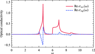
Figure 3: Real part of optical conductivity in the scalar chiral state with $\chi=+\chi_{0}$ at zero temperature. The parameters are set to $J_{\mathrm{K}}=3$, $n_{\mathrm{e}}=0.5$, and $\eta=0.01$.

In the case of $J_{\mathrm{K}}=3$ and $n_{\mathrm{e}}=0.5$, the longitudinal component of the optical conductivity, $\sigma_{xx}(\omega)$, and the transverse component, $\sigma_{xy}(\omega)$, are shown in Fig. 3. Although the direct optical band gap of $\varepsilon_{3}(\bm{k})-\varepsilon_{2}(\bm{k})=4$ is at the $\Gamma$ point, there, the transition dipole moment proportional to $\bm{v}(\bm{k})$ is zero; a significant absorption peak can be seen in $\sigma_{xx}(\omega)$ at $\omega=4.6$, corresponding to the interband transition at the K point. At half filling, since the sum of the Chern numbers of the occupied bands is zero, the transverse conductivity $\sigma_{xy}(\omega)$ vanishes at $\omega=0$, indicating no dc Hall effect. Nonetheless, for $\omega\gtrsim 4$, nonzero $\sigma_{xy}(\omega)$ arises owing to interband transitions, and the sign of $\sigma_{xy}(\omega)$ also depends on the sign of scalar chirality. This can be observed through linear magneto-optical effects, as discussed in Ref. [94]. Even beyond such a linear and perturbative regime, given that the electromagnetic radiation intensity is determined by the expectation value of a one-body electric current operator, we anticipate transverse HHG dependent on scalar chirality.

III.2 Real-time dynamics and HHG

In this section, we examine the real-time dynamics when a continuous wave [Eq. (19)] is applied, and discuss the characteristics of the resulting high harmonic spectrum. First, we consider the case where linearly polarized light parallel to the $x$ axis (i.e., $\psi=0$) is irradiated. The relaxation rate and the optical frequency are set to $\varGamma=0.1$ and $\varOmega=10\times 2\pi/500=0.126$, respectively, with the latter being sufficiently smaller than the optical gap. The ramp time in Eq. (19) and the phase in Eq. (20) are chosen as $\tau=6$ and $\phi=0$, respectively, which do not affect the high harmonic spectrum in a steady state.

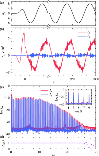
Figure 4: (a), (b) Temporal profiles of (a) the vector potential, $A_{x}(t)$, and (b) the electric currents, $J_{x}(t)$ and $J_{y}(t)$. (c) Power spectra of the electric currents, $I_{x}(\omega)$ and $I_{y}(\omega)$. The inset shows the intensity of low-order harmonics. (d) Phase difference in the transverse current $J_{y}(\omega)$ between states with opposite chiralities, $\delta_{y}=\arg J_{y}(\omega)|_{\chi=-\chi_{0}}-\arg J_{y}(\omega)|_{\chi=+\chi_{0}}$, for odd-order harmonics. The electric field amplitude, frequency, polarization angle, and ramp time are set to $F_{0}=1$, $\varOmega=0.126$, $\psi=0$, and $\tau=6$, respectively.

We show the temporal profiles of the applied vector potential $\bm{A}(t)=(A_{x}(t),0)$ and the electric current density $\bm{J}(t)=(J_{x}(t),J_{y}(t))$ in Figs. 4(a) and 4(b), respectively, when the electric field amplitude is $F_{0}=1$. Given the optical period of $T=2\pi/\varOmega=50$, the system quickly reaches a steady state after a few optical cycles (on a time scale of the order of $\varGamma^{-1}=10$), where not only the longitudinal current $J_{x}$ but also the transverse current $J_{y}$ is induced by the vector potential parallel to the $x$ axis. Although $J_{y}$ is less intense than $J_{x}$, its high-frequency oscillatory components are of similar magnitude to those of $J_{x}$. As becomes clear from the subsequent discussion related to Fig. 4(d), this transverse response is due to $\sigma_{xy}\ (\neq 0)$ arising from scalar chirality, and as shown in Appendix C, it does not occur in the $120^{\mathrm{\circ}}$ Néel state when LP is along a high symmetric direction such as $\psi=0$ and $\pi/6$.

High harmonic spectrum $I(\omega)$ can be obtained using the Fourier transformation of $\bm{J}(t)$. In this study, we extracted real-time data for $500<t\leq 1000$, considering the system to have reached the steady state before $t=500$, and applied the fast Fourier transformation (FFT) to $(1000-500)/\delta t$ data points. The optical frequency of $\varOmega=10\times 2\pi/500$ is consistent with this number of data points, so that the FFT results include data points at frequencies that are exact multiples of $\varOmega$.

Figure 4(c) displays the intensities of the longitudinal and the transverse response, $I_{x}(\omega)$ and $I_{y}(\omega)$, respectively, obtained from $J_{x}(t)$ and $J_{y}(t)$ shown in Fig. 4(b). Since the optical frequency is $\varOmega=0.126$, which is less than $1/30$ of the optical gap, the high harmonic spectrum up to approximately the $200$th order is observed to be clearly separated from a background of $\lesssim 10^{-32}$. Furthermore, as the optical period and the number of data points used for FFT are consistent, sharp peaks appear only at frequencies that are integer multiples of $\varOmega$ as shown in the inset of Fig. 4(c). These high harmonic peaks are observed at odd orders, while the even-order harmonics disappear because of the presence of spatial inversion symmetry. Overall, although the intensity of the transverse component, $I_{y}$, is several orders of magnitude lower than that of the longitudinal component, $I_{x}$, they appear in the same frequency range. Up to about $\omega\lesssim 10$, a plateau appears in the spectrum, which roughly agrees with the frequency range where the optical conductivity is nonzero (see Fig. 3); this is a characteristic widely observed in the HHG in the nonperturbative regime.

Here, we discuss how the transverse response $J_{y}$ changes with respect to the sign of scalar chirality. We confirmed that, for $\chi=-\chi_{0}$, the power spectrum $I_{y}(\omega)$ is exactly the same as in the case of $\chi=+\chi_{0}$ shown in Fig. 4(c) . However, a difference is observed in the phase spectrum. Figure 4(d) shows the difference in the phase component of $J_{y}(\omega)$, defined by $\delta_{y}=\arg J_{y}(\omega)|_{\chi=-\chi_{0}}-\arg J_{y}(\omega)|_{\chi=+\chi_{0}}$, for odd-order harmonics between the cases of $\chi=+\chi_{0}$ and $\chi=-\chi_{0}$. As clearly seen in Fig. 4(d), the transverse component of the odd-order harmonics differ in phases by $\pi$ from each other. This indicates that the sign of the transverse response in the scalar chiral state is inverted by time reversal, implying its association with the presence of scalar chirality, or the Berry curvature.

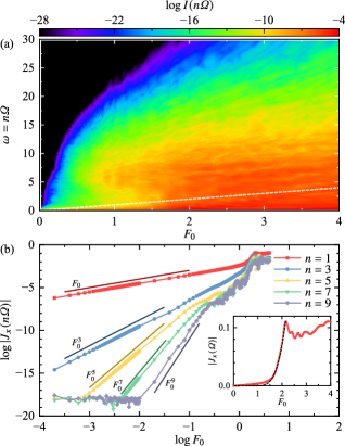
Figure 5: (a) Amplitude dependence of the power spectrum of odd-order harmonics, $I(n\varOmega)\ (n=1,3,\dots)$. The dashed line indicates the upper bound of the Bloch oscillation frequency (see main text). (b) Fourier amplitude of low-order harmonics, $J_{x}(n\varOmega)$, as a function of $F_{0}$. The inset shows $J_{x}(\varOmega)$ on a linear scale, with the dashed curve representing a fitted function, $|J_{x}(\varOmega)|=52.02\exp(-13.22/F_{0})$. The optical frequency and polarization angle are respectively set to $\varOmega=0.126$ and $\psi=0$ in (a) and (b).

We show in Fig. 5 the amplitude dependence of the high harmonic spectrum. Figure 5(a) is a color map displaying the intensity of odd-order harmonics, $I(n\varOmega)$, as a function of the electric field amplitude $F_{0}$. Corresponding to the plateau region observed in Fig. 4(c), the intensity in the region of $\omega\lesssim 10$ is enhanced for $F_{0}\gtrsim 1$. The white dashed line in the figure indicates the upper bound of the Bloch oscillation frequency, which is $\omega=F_{0}$ in the case of $\psi=0$. The frequency domain mainly below this line can include contributions from intraband currents.

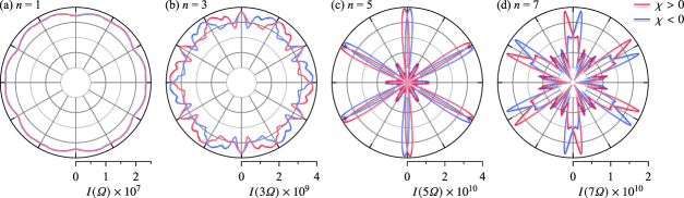
Figure 6: (a)–(d) Polarization angle dependence of the $n$th harmonic intensity $I(n\varOmega)$ for $\chi=+\chi_{0}$ (red) and $\chi=-\chi_{0}$ (blue). The thin dotted curves show the longitudinal component $I_{\parallel}(n\varOmega)$. The electric field amplitude and frequency are set to $F_{0}=1$ and $\varOmega=0.126$, respectively.

The detailed amplitude dependence of the low-order harmonics is plotted in Fig. 5(b). For $F_{0}\lesssim 0.1$, the Fourier amplitude of the $n$th harmonic, $J_{x}(n\varOmega)$, is proportional to the $n$th power of $F_{0}$, indicating that HHG is in the perturbative regime. As $F_{0}$ increases, the higher-order harmonics begin to deviate from the perturbative regime, transitioning to the nonperturbative regime around $F_{0}\sim 1$. The inset of the figure plots the fundamental harmonic amplitude $|J_{x}(\varOmega)|$ on a linear scale. This is well fitted by the exponential function $\exp(-F_{\mathrm{th}}/F_{0})$ with $F_{\mathrm{th}}=13.22$ indicated by the black dashed line, and the excited electron density exhibits similar behavior (not shown), suggesting that interband tunneling excitation dominates for $F_{0}\gtrsim 1.5$. Therefore, for $F_{0}\lesssim 1.5$, tunneling excitation hardly occurs, and the geometrical effects on the tunneling probability discussed in Refs. [106, 107] can be considered negligible.

We examine the polarization angle $\psi$ dependence of the $n$th harmonic intensity for $F_{0}=1$, as shown in Fig. 6. The red and blue lines correspond to the cases of $\chi=+\chi_{0}$ and $\chi=-\chi_{0}$, respectively. For the first-order harmonic, the difference due to the chirality sign is almost negligible, and it is approximately independent of the polarization angle. This partially inherits the property that, in the current system with six-fold symmetry, a linear optical response exhibits continuous rotational symmetry. On the other hand, for the third and higher harmonics, not only does a significant dependence on the incident polarization angle appear, but clear differences are observed depending on the sign of scalar chirality. As previously mentioned, the chirality sign only changes the sign of the Berry curvature and does not alter the energy band structure; hence, this chirality dependence is attributed to purely geometrical effects.

The polarization angle dependence reflecting the sign of scalar chirality is naively expected to arise from the anomalous velocity of intraband currents, as discussed in the literature [80, 81, 82, 83, 84, 85, 86] for systems where spatial inversion symmetry is broken. The intraband current carried by an electron with momentum $\bm{k}$ in the $n$th band is proportional to

$$\dot{\bm{r}}_{n}=\partial_{\bm{k}}\varepsilon_{n}(\bm{k})+\bm{F}(t)\times\bm{B}_{n}(\bm{k}),$$ (26)

where $\bm{r}$ is the position of the electron, and the second term is called the anomalous velocity. Note that the anomalous velocity term always produces a current perpendicular to the electric field $\bm{F}$. Therefore, to extract the contribution of the transverse response, the power spectrum $I(\omega)$ is decomposed into components parallel and perpendicular to $\bm{F}$, denoted as $I_{\parallel}(\omega)$ and $I_{\perp}(\omega)$, respectively. These are related to $I_{x}(\omega)$ and $I_{y}(\omega)$ through the relations:

$$I_{\parallel} =I_{x}\cos^{2}\psi+2\sqrt{I_{x}I_{y}}\cos\psi\sin\psi\cos\delta+I_{y}\sin^{2}\psi,$$ (27)

$$I_{\perp} =I_{x}\sin^{2}\psi-2\sqrt{I_{x}I_{y}}\cos\psi\sin\psi\cos\delta+I_{y}\cos^{2}\psi,$$ (28)

with $\delta(\omega)=\arg J_{y}(\omega)-\arg J_{x}(\omega)$. The thin dotted curves in Fig. 6 show the polarization angle dependence of the intensity of the parallel component $I_{\parallel}(\omega)=I(\omega)-I_{\perp}(\omega)$. Contrary to expectation, for any $\psi$, we observe that $I_{\parallel}\approx I$, indicating that the anomalous velocity (and a component of $\partial_{\bm{k}}\varepsilon_{n}(\bm{k})$ that is perpendicular to $\bm{k}(t)=\bm{k}-\bm{A}(t)$) in the intraband current cannot explain the observed dependence on the sign of scalar chirality. Thus, in the following section, we consider interband currents associated with the recombination of electron–hole pairs.

III.3 Electron–hole dynamics in real space

In the previous section, as shown in Fig. 6, it was revealed that the polarization angle dependence of harmonic intensity changes with the sign of scalar chirality, and that it is mostly due to the contribution of an electric current component parallel to the electric field. Since it is currently difficult to fully understand this cause microscopically, in this section, we discuss interband currents by analyzing a real-space trajectory of an electron–hole pair excited at a wavenumber point $\bm{k}=\bm{k}_{0}$.

At half filling, optical driving primarily excites electrons into the third lowest band $\varepsilon_{3}(\bm{k})$, while creating holes in the second band $\varepsilon_{2}(\bm{k})$. Interband currents are induced when these electrons and holes recombine. In the saddle-point approximation [70, 71, 72, 73, 74], this condition is expressed as $\|\delta\bm{r}\|=0$, where $\delta\bm{r}$ represents the relative displacement of the electron–hole pair excited at time $t=0$. This displacement is given by

$$\delta\bm{r}(t)=\int_{0}^{t}\delta\dot{\bm{r}}(t^{\prime})\,\mathrm{d}t^{\prime},$$ (29)

where $\delta\dot{\bm{r}}$ denotes the relative velocity of the electron–hole pair with momentum $\bm{k}$:

$$\delta\dot{\bm{r}} =\partial_{\bm{k}}[\varepsilon_{3}(\bm{k})-\varepsilon_{2}(\bm{k})]+\bm{F}(t)\times[\bm{B}_{3}(\bm{k})-\bm{B}_{2}(\bm{k})].$$ (30)

The optical vector potential is introduced through the Peierls substitution: $\bm{k}(t)=\bm{k}_{0}+\bm{A}(0)-\bm{A}(t)$ with $\bm{A}(t)=-(\bm{F}_{0}/\varOmega)\sin(\varOmega t-\phi)$. Therefore, by finding the phase $\phi$ for which $\|\delta\bm{r}\|=0$ at time $t>0$, we can determine the real-space trajectory of the electron–hole pair until recombination.

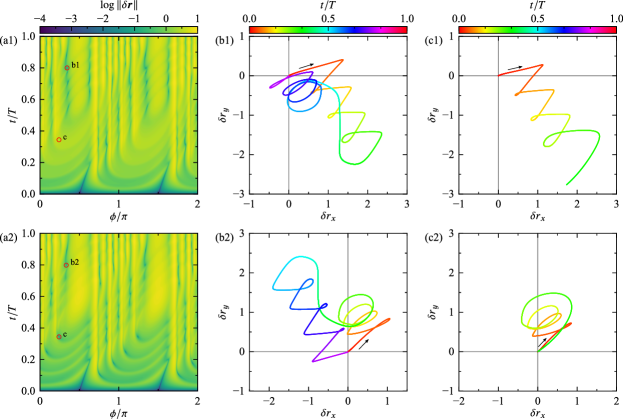
Figure 7: Real-space dynamics of electron–hole pair excited at $t=0$ with $\bm{k}=(0,0)$, for $\chi=+\chi_{0}$ (upper panels) and $\chi=-\chi_{0}$ (lower panels). The electric field amplitude, frequency, polarization angle are set to $F_{0}=1$, $\varOmega=0.126$, and $\psi=32^{\mathrm{\circ}}$, respectively. (a) Color map of the norm of the relative displacement, $\|\delta\bm{r}\|$, in the $\phi$-$t$ plane. (b) Real-space trajectory of $\delta\bm{r}$ until recombination for an initial phase indicated by the red circle, ‘b1’ and ‘b2’, in (a). (c) Same as (b) but for a different initial phase indicated by ‘c’ in (a); point ‘c’ in (a1) is not a local minimum of $\|\delta\bm{r}\|$, and thus in (c1), the pair does not recombine (see main text).

Analyzing all trajectories of electron–hole pairs for every $\bm{k}_{0}$ would only complicate the problem. Thus, here, we specifically show representative cases for a pair excited at $\bm{k}_{0}=(0,0)$, that is, at the $\Gamma$ point. Figure 7(a) displays the relative displacement $\|\delta\bm{r}\|$ on a logarithmic scale as a function of the initial phase $\phi$ and time $t$, with Fig. 7(a1) for $\chi=+\chi_{0}$ and Fig. 7(a2) for $\chi=-\chi_{0}$. The polarization angle is set to $\psi=32^{\mathrm{\circ}}$, for which the $5$th-order harmonic intensity for $\chi=+\chi_{0}$ nearly reaches its maximum [see Fig. 6(c)]. Overall, both cases exhibit similar behaviors, but, reflecting the sign of scalar chirality (i.e., the sign of the Berry curvature), the details differ. There are specifically two cases in which the electron–hole pair can recombine: (i) for both $\chi=+\chi_{0}$ and $\chi=-\chi_{0}$, the pair recombines at almost the same phase $\phi$ and time $t$ (indicated by points ‘b1’ and ‘b2’), and (ii) the pair recombines only for either $\chi=+\chi_{0}$ or $\chi=-\chi_{0}$ (indicated by point ‘c’). We discuss these two cases in detail.

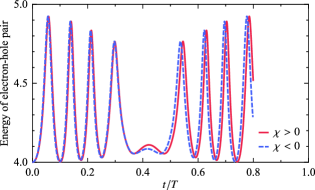
Figure 8: Temporal profiles of the energy of electron–hole pair until the recombination, with the initial phases indicated by ‘b1’ for $\chi=+\chi_{0}$ and by ‘b2’ for $\chi=-\chi_{0}$ in Figs. 7(a1) and 7(a2) (see main text). The other parameters are the same as those in Fig. 7.

Case (i). The phase and the recombination time of points ‘b1’ and ‘b2’ in Figs. 7(a1) and 7(a2) are $\phi/\pi=0.344$ and $t/T=0.800$ for $\chi=+\chi_{0}$, and $\phi/\pi=0.333$ and $t/T=0.799$ for $\chi=-\chi_{0}$. Here, $T=2\pi/\varOmega=50$ represents the optical period. The corresponding trajectories in real space are shown in Figs. 7(b1) and 7(b2). Although these trajectories are close to what would be expected if the time was reversed for the other, the contribution from the anomalous velocity term modifies the conditions for recombination. This results in a slight difference in a recombination energy. Figure 8 shows the temporal profile of the electron–hole pair’s energy, $\varepsilon_{3}\text{{(}}\bm{k}(t)\text{{)}}-\varepsilon_{2}\text{{(}}\bm{k}(t)\text{{)}}$, where we in fact observe the slight difference. Thus, in this case, while the electron–hole pair recombines for both $\chi=+\chi_{0}$ and $\chi=-\chi_{0}$, their different recombination energies at $t\approx 0.8$ yield a different harmonic intensity.

Case (ii). When $\phi/\pi=0.2416$ and $t/T=0.344$, indicated as ‘c’ in Fig. 7(a), pair recombination occurs only for $\chi=-\chi_{0}$. The trajectories for this case are shown in Figs. 7(c1) and 7(c2). For $\chi=+\chi_{0}$, the electron–hole pair does not return to the coordinate origin, and thus, this pair does not contribute to interband currents.

From the two cases above, the reason why the dependence of chirality sign, as shown in Fig. 6, appears as a longitudinal response can be inferred to be due to the difference in the dynamics of electron–hole pairs in real space. This difference is caused by the anomalous velocity, which also changes the recombination conditions. Furthermore, even in a case where recombination occur for both $\chi=+\chi_{0}$ and $\chi=-\chi_{0}$, the difference in the recombination energy results in variations in harmonic intensity. However, it is also important to note that the analysis conducted here is significantly simplified and does not consider crucial factors such as temporal changes in the carrier density and interference with other pairs excited at different $\bm{k}$’s, necessitating more comprehensive analyses as conducted in Ref. [89] in future work.

III.4 HHG with parameters for real materials

In the previous sections, we discussed the case where $J_{\mathrm{K}}=3$ and $n_{\mathrm{e}}=0.5$. Recently, some experiments reported that the four-sublattice scalar chiral state is realized in $\mathrm{CoTa_{3}S_{6}}$ and $\mathrm{CoNb_{3}S_{6}}$ [99, 100, 101]. Here, we discuss the high harmonic spectrum and its polarization angle dependence for parameters close to these materials, with $J_{\mathrm{K}}=0.4$ and $n_{\mathrm{e}}=0.75$. We will see that the aforementioned conclusion regarding the dominance of the longitudinal response depending on chirality sign also holds in this case.

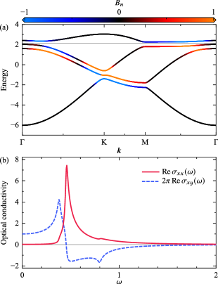
Figure 9: (a) Energy band structure $\varepsilon_{n}(\bm{k})$ for $J_{\mathrm{K}}=0.4\ (\chi=+\chi_{0})$. The color variation along the lines indicates the Berry curvature $B_{n}(\bm{k})$. The gray horizontal line shows the chemical potential $\mu=2.137$ for $n_{\mathrm{e}}=0.75$. (b) Real part of optical conductivity in the scalar chiral state with $\chi=+\chi_{0}$ at zero temperature. The parameters are set to $J_{\mathrm{K}}=0.4$, $n_{\mathrm{e}}=0.75$, and $\eta=0.01$.

Before moving on to the discussion of HHG, we present the equilibrium properties. Figure 9(a) shows the energy band structure and Berry curvature in the ground state for $J_{\mathrm{K}}=0.4$. Only at three-quarter filling ($n_{\mathrm{e}}=0.75$), the ground state is insulating. The optical conductivity is shown in Fig. 9(b). A significant absorption peak in $\sigma_{xx}(\omega)$ is observed near $\omega=0.42$, corresponding to the transition between the upper two bands on the $\Gamma$–M line. Hereafter, the optical frequency will continue to be set at $\varOmega=0.126$, which is still lower than the optical gap. Furthermore, reflecting the Berry curvature, the optical Hall conductivity $\sigma_{xy}(\omega)$ also appears, and it reaches the quantized value of $+e^{2}/(2\pi\hbar)$ in the dc limit ($\omega\to 0$).

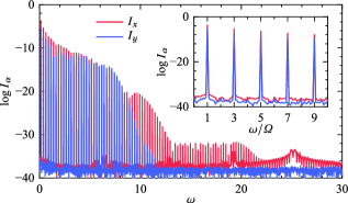
Figure 10: Power spectra of the electric currents, $I_{x}(\omega)$ and $I_{y}(\omega)$. The inset shows the intensity of low-order harmonics. The parameters are set to $J_{\mathrm{K}}=0.4$, $n_{\mathrm{e}}=0.75$, $F_{0}=0.1$, and $\varOmega=0.126$.

In Fig. 10, we show the power spectrum $I_{\alpha}(\omega)$ for $F_{0}=0.1$ and $\varOmega=0.126$. Similarly to Fig. 4(c), the transverse response $I_{y}$ appears with the same order of magnitude as or several orders of magnitude smaller than the longitudinal response $I_{x}(\omega)$. As the energy range from the bottom to the top band edge is approximately $9$ [see Fig. 9(a)], we observe the cutoff energy (i.e., the upper end of the plateau region) to be at the same energy $\sim 8$ in the spectrum. While harmonic peaks and a plateau are also seen in $I_{x}$ in the high energy region of $\omega\gtrsim 9$, interpreting their origin is difficult; we speculate that they may be artifacts of numerical calculations.

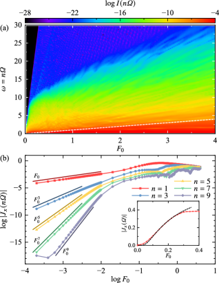
Figure 11: (a) Amplitude dependence of the power spectrum of odd-order harmonics, $I(n\varOmega)\ (n=1,3,\dots)$. The dashed line indicates the upper bound of the Bloch oscillation frequency. (b) Fourier amplitude of low-order harmonics, $J_{x}(n\varOmega)$, as a function of $F_{0}$. The inset shows $J_{x}(\varOmega)$ on a linear scale, with the dashed curve representing a fitted function, $|J_{x}(\varOmega)|=0.7709\exp(-0.2043/F_{0})$. The parameters are set to $J_{\mathrm{K}}=0.4$, $n_{\mathrm{e}}=0.75$, $\varOmega=0.126$, and $\psi=0$ in (a) and (b).

Figure 11(a) shows the color map of the intensity of odd-order harmonics as a function of the electric field amplitude. Reflecting the observation in Fig. 2(b) that the optical gap is about an order of magnitude smaller than that in the case of $J_{\mathrm{K}}=3$, the transition from the perturbative to the nonperturbative region occurs at a lower $F_{0}$. The intensity $I(\omega)$ is particularly strong in the region of $\omega\lesssim 10$, consistent with the bandwidth of the electrons. In addition, in the region below the white dashed line in Fig. 11(a), a significant contribution from intraband currents associated with the Bloch oscillation is also apparent.

The $F_{0}$ dependence of the harmonic intensities up to the $9$th order is shown in Fig. 11(b). For the fundamental harmonics ($n=1$), a deviation from the perturbative line $J_{x}(\varOmega)\propto F_{0}$ can be seen above $F_{0}\sim 0.1$, and for higher harmonics, this deviation can be seen at a smaller $F_{0}$. To consider the same situation as in the previous sections, the following discusses the polarization angle dependence for $F_{0}=0.1$.

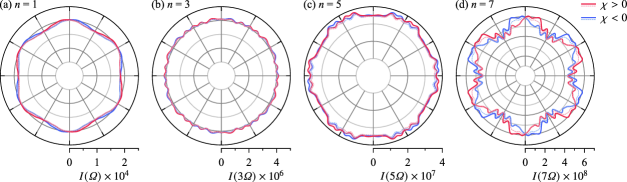
Figure 12: (a)–(d) Polarization angle dependence of the $n$th harmonic intensity $I(n\varOmega)$ for $\chi=+\chi_{0}$ (red) and $\chi=-\chi_{0}$ (blue). The thin dotted curves show the longitudinal component $I_{\parallel}(n\varOmega)$. The parameters are set to $J_{\mathrm{K}}=0.4$, $n_{\mathrm{e}}=0.75$, $F_{0}=0.1$, and $\varOmega=0.126$.

We present the polarization angle dependence of harmonic intensity in Fig. 12. Similarly to the case of $J_{\mathrm{K}}=3$ and $n_{\mathrm{e}}=0.5$, the harmonic intensities depend on the polarization anlge $\psi$, reflecting the sign of chirality. However, for harmonics up to the $5$th order at $F_{0}=0.1$, the significant angle dependence shown in Figs. 6(c) and 6(d) are not observed. Additionally, the thin dashed lines in the figure indicates the longitudinal intensity $I_{\parallel}$ parallel to the electric field $\bm{F}_{0}$, which, as in the previous case, satisfies $I_{\parallel}\approx I$, indicating the dominance of the longitudinal response depending on the chirality sign. Therefore, we consider that the results and discussions in the previous sections do not qualitatively depend on details such as model parameters or electron density.

IV Discussion

In Sec. III, we have focused particularly on a case where the optical frequency is significantly lower than the energy gap. Previous studies [80, 81, 82, 83, 84, 85, 86] have mainly discussed the effects of anomalous velocity in intraband currents; however, our results reveal that despite the dominance of the longitudinal response over the transverse response, the polarization angle dependence of harmonic intensity strongly reflects the sign of scalar chirality. While this behavior might also be observed in systems with broken spatial inversion symmetry and nonzero Berry curvature, note that the sign of the Berry curvature can be easily switched by an external magnetic field in systems with broken time reversal symmetry.

It is also a natural question whether the anomalous velocity term in intraband currents (i.e., the transverse response) could dominate in the present system. In Appendix A, we show results on the polarization angle dependence in the case of near-resonant driving. There, indeed, the transverse response can become comparable to or greater than the longitudinal response. Besides, it is noteworthy that the longitudinal response still exhibits a dependence on the chirality sign. In addition, Appendices B and C respectively present brief summaries of the high harmonic spectrum in the case with circular polarization driving, and of the polarization angle dependence of the harmonic intensities in the $120^{\mathrm{\circ}}$ Néel state, where the Berry curvature is zero.

As already mentioned, the linear optical Hall effect with topological spin textures has been discussed in the literature [92, 93, 94, 95, 96]. In systems with six-fold symmetry like the one considered here, the linear conductivity exhibits continuous rotational symmetry, and thus shows no polarization angle dependence, unlike what is observed in Figs. 6 and 12. Therefore, to verify the results presented in this paper, experiments need to be conducted on single crystals without grain boundaries. Additionally, the scalar chiral state in $\mathrm{CoTa_{3}S_{6}}$ and $\mathrm{CoNb_{3}S_{6}}$ is metallic [99, 100, 101], leading to the enhancement of the intraband-current response. Thus, examining harmonics in a frequency range higher than the Bloch oscillation frequency would facilitate a clearer observation of the contribution from interband currents.

V Summary

In this paper, we numerically analyzed HHG arising from electrons in the spin scalar chiral state. Reflecting the presence of the Berry curvature, the transverse response emerges, which is of the same order of magnitude as, or several orders of magnitude smaller than, the longitudinal response; its phase inversion depends on the sign of scalar chirality. Furthermore, we observed a marked variation in harmonic intensity with respect to the incident polarization angle, dependent on the chirality sign, with the dominant component being the longitudinal response rather than the transverse one. Since the anomalous velocity term in intraband currents produces only the transverse currents, this longitudinal response can be attributed to interband currents induced by the recombination of electron–hole pairs whose trajectories are modulated by the anomalous velocity. This modulation changes the recombination energies of the pairs and thus can alter the spectrum of interband currents. These results indicate that the magnetic structure with scalar chirality is, in fact, reflected in the high harmonic spectrum through the electron dynamics, which can be verified in experiments with materials such as $\mathrm{CoTa_{3}S_{6}}$ and $\mathrm{CoNb_{3}S_{6}}$, where the sign of scalar chirality can be switched by a magnetic field. Further research is expected to extend to HHG and HSG in systems with other topological spin textures, such as skyrmion lattice and hedgehog lattice states. Additionally, while the localized spins are fixed in this study, considering the dynamics resulting from the coupling between electrons and magnons would present an interesting direction [102, 108, 109, 110].

Appendix A Near-resonant driving

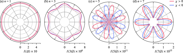
Figure 13: (a)–(d) Polarization angle dependence of the $n$th harmonic intensity $I(n\varOmega)$ for $\chi=+\chi_{0}$ (red) and $\chi=-\chi_{0}$ (blue). The thin dotted curves show the longitudinal component $I_{\parallel}(n\varOmega)$, and $I_{\parallel}(5\varOmega)$ is additionally shaded for visibility. The electric field amplitude and frequency are set to $F_{0}=1$ and $\varOmega=4.02$, respectively.

In the main text, we set the optical frequency to $\varOmega=0.126$ and discussed the situation where it is significantly lower than the optical gap of $4$ for $J_{\mathrm{K}}=3$. Here, we present in Fig. 13 the polarization angle dependence of harmonic intensity for a near-resonant case with $\varOmega=320\times 2\pi/500=4.02$ and $F_{0}=1$. Since $\varOmega$ is near resonant, the intensity of the fundamental harmonic is six orders of magnitude larger than that in Fig. 6(a), but the angle dependence is small, suggesting that its deviation from the perturbative regime is small. The higher order harmonics show a pronounced $\psi$ dependence similar to the case of $\varOmega=0.126$, and changes relative to the sign of scalar chirality can be similarly observed. Among the higher order harmonics shown in Fig. 13, the $3$rd- and $7$th-order longitudinal response satisfies $I_{\parallel}\approx I$, but for the $5$th harmonic, the transverse response $I_{\perp}$ becomes comparable to or greater than $I_{\parallel}$. This large transverse response can be attributed to the anomalous velocity term in intraband currents, as discussed in the literature. Nevertheless, $I_{\parallel}$ still clearly depends on the chirality sign, indicating that $I(\omega)$ contains interband-current contributions discussed in Sec. III.3.

Appendix B Circular polarization driving

Here, we briefly discuss HHG when circularly polarized light defined in Eq. (23) is applied. Before that, we present the relationship between the parameters of an ellipse and the electric current’s amplitude and phase. When the electric current corresponding to the $n$th harmonic is given by

$$J_{\alpha}(t)=J_{0,\alpha}\cos(n\varOmega t-\phi_{\alpha})$$ (31)

with $J_{0,\alpha}=|J_{\alpha}(n\varOmega)|$ and $\phi_{\alpha}=\arg J_{\alpha}(n\varOmega)$, the trajectory on the $J_{x}$-$J_{y}$ plane is an ellipse. Its semi-major axis $J_{+}$ and semi-minor axis $J_{-}$ are respectively given by

$$J_{+}=\max\{\tilde{J}_{x},\tilde{J}_{y}\},\quad J_{-}=\operatorname{sgn}(\delta)\min\{\tilde{J}_{x},\tilde{J}_{y}\},$$ (32)

where $\delta=\phi_{y}-\phi_{x}$ represents the relative phase, $\operatorname{sgn}$ denotes a sign function, and $\tilde{J}_{x}$ and $\tilde{J}_{y}$ are defined by

$$\tilde{J}_{x} =|\sin\delta\,|\left[\frac{\cos^{2}\varphi}{J_{0,x}^{2}}-\frac{\sin 2\varphi\cos\delta}{J_{0,x}J_{0,y}}+\frac{\sin^{2}\varphi}{J_{0,y}^{2}}\right]^{-\frac{1}{2}},$$ (33)

$$\tilde{J}_{y} =|\sin\delta\,|\left[\frac{\sin^{2}\varphi}{J_{0,x}^{2}}+\frac{\sin 2\varphi\cos\delta}{J_{0,x}J_{0,y}}+\frac{\cos^{2}\varphi}{J_{0,y}^{2}}\right]^{-\frac{1}{2}}.$$ (34)

Here, $\varphi$ represents the inclination angle of the ellipse’s major axis with respect to the $x$ axis, which is given by

$$\varphi=\frac{1}{2}\arctan\frac{2J_{0,x}J_{0,y}\cos\delta}{J_{0,x}^{2}-J_{0,y}^{2}}.$$ (35)

The ellipticity $\epsilon$ is defined by

$$\epsilon=-\frac{J_{-}}{J_{+}},$$ (36)

such that it equals $+1$ for RCP and $-1$ for LCP.

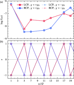
Figure 14: (a) Power spectrum $I(\omega)$ and (b) ellipticity $\epsilon$, for $(6l\pm 1)$th-order harmonics. RCP and LCP correspond to $\epsilon=+1$ and $\epsilon=-1$, respectively. The parameters are set to $J_{\mathrm{K}}=3$, $n_{\mathrm{e}}=0.5$, $F_{0}=0.1$, and $\varOmega=0.126$.

Figure 14(a) shows the power spectrum $I(\omega)$ for harmonics with intensity sufficiently separated from the background ($\lesssim 10^{-30}$). It is established that the allowed harmonics for a given crystal symmetry and optical-field waveform are described by a theory of dynamical symmetry [111, 112, 113, 35, 114, 115]. In the present system, which exhibits six-fold symmetry, only the $(6l\pm 1)$th-order harmonics ($l\in\mathbb{Z}$) are allowed when circularly polarized light is applied, and our results are in agreement with this theoretical prediction. Additionally, Fig. 14(b) demonstrates that the ellipticity $\epsilon$ of each harmonic is determined solely by the handedness of the circular polarization, regardless of the sign of chirality. Furthermore, a kind of circular dichroism is observed; that is, for $\chi=+\chi_{0}$, the intensity of the $5$th- to $13$th-order harmonics under LCP is more pronounced than those under RCP, and this difference in intensities is inverted when the sign of chirality is altered.

Appendix C Comparison with the 120^∘ Néel state

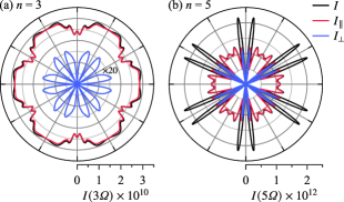
Figure 15: Polarization angle dependence of the (a) $3$rd and (b) $5$th harmonic intensity. The red and blue lines represent the longitudinal ($I_{\parallel}$) and transverse ($I_{\perp}$) component, respectively. For visibility, $I_{\perp}(3\varOmega)$ in (a) is multiplied by $20$.

The $120^{\mathrm{\circ}}$ Néel state exhibits a three-sublattice magnetic order, which is stabilized at $n_{\mathrm{e}}=0.5$ in the present model [98]. The vector of the $m$th sublattice spin is defined by $\bm{S}_{m}=(\cos\theta_{m},\sin\theta_{m},0)$ with $\theta_{1}=0$, $\theta_{2}=2\pi/3$, and $\theta_{3}=-2\pi/3$. Given this configuration, the electron system is invariant under the combination of a mirror reflection with respect to the $xy$ plane and the time reversal operation; thereby the Berry curvature $\bm{B}_{n}(\bm{k})$ satisfies $B_{n}^{z}(-k_{x},-k_{y},k_{z})=-B_{n}^{z}(k_{x},k_{y},k_{z})$ [116], or in two dimensions, $B_{n}(-k_{x},-k_{y})=-B_{n}(k_{x},k_{y})$. Additionally, the presence of spatial inversion symmetry imposes $B_{n}(-k_{x},-k_{y})=B_{n}(k_{x},k_{y})$. Therefore, the Berry curvature $B_{n}(\bm{k})$ turns out to be zero for any $\bm{k}$. In the case with $J_{\mathrm{K}}=3$ and $n_{\mathrm{e}}=0.5$ as adopted in the main text, the ground state is insulating, and the optical gap is $2J_{\mathrm{K}}=6$.

In Fig. 15, we present the polarization angle dependence of the $3$rd- and $5$th-order harmonic intensities for $F_{0}=1$ and $\varOmega=0.126$, along with their longitudinal and transverse components. Similarly to the case in the four-sublattice scalar chiral state, six-fold symmetric harmonic intensity is observed, with the $5$th harmonic showing more pronounced angle dependence. The transverse component $I_{\perp}$, shown in blue lines in the figure, appears except in the high symmetric directions such as $\psi=0$ and $\psi=\pi/6$, and it does not depend on the sign of $J_{\mathrm{K}}$ unlike in the scalar chiral state. Such transverse response can be attributed to the first term of Eq. (26), $\partial_{\bm{k}}\varepsilon_{n}(\bm{k})$, having components that are not parallel to the momentum $\bm{k}$.

References

- Agostini and DiMauro [2004] P. Agostini and L. F. DiMauro, The physics of attosecond light pulses, Rep. Prog. Phys. 67, 813 (2004).
- Gallmann et al. [2012] L. Gallmann, C. Cirelli, and U. Keller, Attosecond Science: Recent Highlights and Future Trends, Annu. Rev. Phys. Chem. 63, 447 (2012).
- Krausz and Ivanov [2009] F. Krausz and M. Ivanov, Attosecond physics, Rev. Mod. Phys. 81, 163 (2009).
- Kruchinin et al. [2018] S. Y. Kruchinin, F. Krausz, and V. S. Yakovlev, Colloquium: Strong-field phenomena in periodic systems, Rev. Mod. Phys. 90, 021002 (2018).
- Ghimire and Reis [2019] S. Ghimire and D. A. Reis, High-harmonic generation from solids, Nat. Phys. 15, 10 (2019).
- Amini et al. [2019] K. Amini, J. Biegert, F. Calegari, A. Chacón, M. F. Ciappina, A. Dauphin, D. K. Efimov, C. Figueira de Morisson Faria, K. Giergiel, P. Gniewek, A. S. Landsman, M. Lesiuk, M. Mandrysz, A. S. Maxwell, R. Moszyński, L. Ortmann, J. Antonio Pérez-Hernández, A. Picón, E. Pisanty, J. Prauzner-Bechcicki, K. Sacha, N. Suárez, A. Zaïr, J. Zakrzewski, and M. Lewenstein, Symphony on strong field approximation, Rep. Prog. Phys. 82, 116001 (2019).
- Li et al. [2023] L. Li, P. Lan, X. Zhu, and P. Lu, High harmonic generation in solids: particle and wave perspectives, Rep. Prog. Phys. 86, 116401 (2023).
- Borsch et al. [2023] M. Borsch, M. Meierhofer, R. Huber, and M. Kira, Lightwave electronics in condensed matter, Nat. Rev. Mater. 8, 668 (2023).
- Na et al. [2023] M. Na, A. K. Mills, and D. J. Jones, Advancing time- and angle-resolved photoemission spectroscopy: The role of ultrafast laser development, Phys. Rep. 1036, 1 (2023).
- de la Torre et al. [2021] A. de la Torre, D. M. Kennes, M. Claassen, S. Gerber, J. W. McIver, and M. A. Sentef, Colloquium: Nonthermal pathways to ultrafast control in quantum materials, Rev. Mod. Phys. 93, 041002 (2021).
- Filippetto et al. [2022] D. Filippetto, P. Musumeci, R. K. Li, B. J. Siwick, M. R. Otto, M. Centurion, and J. P. F. Nunes, Ultrafast electron diffraction: Visualizing dynamic states of matter, Rev. Mod. Phys. 94, 045004 (2022).
- Boschini et al. [2024] F. Boschini, M. Zonno, and A. Damascelli, Time-resolved ARPES studies of quantum materials, Rev. Mod. Phys. 96, 015003 (2024).
- Oka and Kitamura [2019] T. Oka and S. Kitamura, Floquet Engineering of Quantum Materials, Annu. Rev. Condens. Matter Phys. 10, 387 (2019).
- [14] Y. Murakami, D. Golež, M. Eckstein, and P. Werner, Photo-induced nonequilibrium states in Mott insulators, arXiv:2310.05201 .
- Ghimire et al. [2011] S. Ghimire, A. D. DiChiara, E. Sistrunk, P. Agostini, L. F. DiMauro, and D. A. Reis, Observation of high-order harmonic generation in a bulk crystal, Nat. Phys. 7, 138 (2011).
- Schubert et al. [2014] O. Schubert, M. Hohenleutner, F. Langer, B. Urbanek, C. Lange, U. Huttner, D. Golde, T. Meier, M. Kira, S. W. Koch, and R. Huber, Sub-cycle control of terahertz high-harmonic generation by dynamical Bloch oscillations, Nat. Photonics 8, 119 (2014).
- Hohenleutner et al. [2015] M. Hohenleutner, F. Langer, O. Schubert, M. Knorr, U. Huttner, S. W. Koch, M. Kira, and R. Huber, Real-time observation of interfering crystal electrons in high-harmonic generation, Nature 523, 572 (2015).
- Garg et al. [2016] M. Garg, M. Zhan, T. T. Luu, H. Lakhotia, T. Klostermann, A. Guggenmos, and E. Goulielmakis, Multi-petahertz electronic metrology, Nature 538, 359 (2016).
- Langer et al. [2016] F. Langer, M. Hohenleutner, C. P. Schmid, C. Poellmann, P. Nagler, T. Korn, C. Schüller, M. S. Sherwin, U. Huttner, J. T. Steiner, S. W. Koch, M. Kira, and R. Huber, Lightwave-driven quasiparticle collisions on a subcycle timescale, Nature 533, 225 (2016).
- Langer et al. [2017] F. Langer, M. Hohenleutner, U. Huttner, S. W. Koch, M. Kira, and R. Huber, Symmetry-controlled temporal structure of high-harmonic carrier fields from a bulk crystal, Nat. Photonics 11, 227 (2017).
- Yoshikawa et al. [2017] N. Yoshikawa, T. Tamaya, and K. Tanaka, High-harmonic generation in graphene enhanced by elliptically polarized light excitation, Science 356, 736 (2017).
- Mrudul and Dixit [2021] M. S. Mrudul and G. Dixit, High-harmonic generation from monolayer and bilayer graphene, Phys. Rev. B 103, 094308 (2021).
- Xia et al. [2021] P. Xia, T. Tamaya, C. Kim, F. Lu, T. Kanai, N. Ishii, J. Itatani, H. Akiyama, and T. Kato, High-harmonic generation in GaAs beyond the perturbative regime, Phys. Rev. B 104, L121202 (2021).
- Tamaya et al. [2016] T. Tamaya, A. Ishikawa, T. Ogawa, and K. Tanaka, Diabatic Mechanisms of Higher-Order Harmonic Generation in Solid-State Materials under High-Intensity Electric Fields, Phys. Rev. Lett. 116, 016601 (2016).
- Sato et al. [2021] S. A. Sato, H. Hirori, Y. Sanari, Y. Kanemitsu, and A. Rubio, High-order harmonic generation in graphene: Nonlinear coupling of intraband and interband transitions, Phys. Rev. B 103, L041408 (2021).
- Murakami and Schüler [2022] Y. Murakami and M. Schüler, Doping and gap size dependence of high-harmonic generation in graphene: Importance of consistent formulation of light-matter coupling, Phys. Rev. B 106, 035204 (2022).
- Murakami et al. [2023] Y. Murakami, K. Nagai, and A. Koga, Efficient control of high harmonic terahertz generation in carbon nanotubes using the Aharonov-Bohm effect, Phys. Rev. B 108, L241202 (2023).
- Floss et al. [2018] I. Floss, C. Lemell, G. Wachter, V. Smejkal, S. A. Sato, X.-M. Tong, K. Yabana, and J. Burgdörfer, Ab initio multiscale simulation of high-order harmonic generation in solids, Phys. Rev. A 97, 011401 (2018).
- Sekiguchi et al. [2023] F. Sekiguchi, M. Sakamoto, K. Nakagawa, H. Tahara, S. A. Sato, H. Hirori, and Y. Kanemitsu, Enhancing high harmonic generation in GaAs by elliptically polarized light excitation, Phys. Rev. B 108, 205201 (2023).
- Kono et al. [1997] J. Kono, M. Y. Su, T. Inoshita, T. Noda, M. S. Sherwin, S. J. Allen, Jr., and H. Sakaki, Resonant Terahertz Optical Sideband Generation from Confined Magnetoexcitons, Phys. Rev. Lett. 79, 1758 (1997).
- Zaks et al. [2012] B. Zaks, R. B. Liu, and M. S. Sherwin, Experimental observation of electron–hole recollisions, Nature 483, 580 (2012).
- Langer et al. [2018] F. Langer, C. P. Schmid, S. Schlauderer, M. Gmitra, J. Fabian, P. Nagler, C. Schüller, T. Korn, P. G. Hawkins, J. T. Steiner, U. Huttner, S. W. Koch, M. Kira, and R. Huber, Lightwave valleytronics in a monolayer of tungsten diselenide, Nature 557, 76 (2018).
- Uchida et al. [2018] K. Uchida, T. Otobe, T. Mochizuki, C. Kim, M. Yoshita, K. Tanaka, H. Akiyama, L. N. Pfeiffer, K. W. West, and H. Hirori, Coherent detection of THz-induced sideband emission from excitons in the nonperturbative regime, Phys. Rev. B 97, 165122 (2018).
- Borsch et al. [2020] M. Borsch, C. P. Schmid, L. Weigl, S. Schlauderer, N. Hofmann, C. Lange, J. T. Steiner, S. W. Koch, R. Huber, and M. Kira, Super-resolution lightwave tomography of electronic bands in quantum materials, Science 370, 1204 (2020).
- Nagai et al. [2020] K. Nagai, K. Uchida, N. Yoshikawa, T. Endo, Y. Miyata, and K. Tanaka, Dynamical symmetry of strongly light-driven electronic system in crystalline solids, Commun. Phys. 3, 137 (2020).
- Costello et al. [2021] J. B. Costello, S. D. O’Hara, Q. Wu, D. C. Valovcin, L. N. Pfeiffer, K. W. West, and M. S. Sherwin, Reconstruction of Bloch wavefunctions of holes in a semiconductor, Nature 599, 57 (2021).
- [37] K. Uchida and K. Tanaka, High harmonic interferometer:For probing sub-laser-cycle electron dynamics in solids, arXiv:2304.14704 .
- Silva et al. [2018] R. E. F. Silva, I. V. Blinov, A. N. Rubtsov, O. Smirnova, and M. Ivanov, High-harmonic spectroscopy of ultrafast many-body dynamics in strongly correlated systems, Nat. Photonics 12, 266 (2018).
- Murakami et al. [2018] Y. Murakami, M. Eckstein, and P. Werner, High-Harmonic Generation in Mott Insulators, Phys. Rev. Lett. 121, 057405 (2018).
- Imai et al. [2020] S. Imai, A. Ono, and S. Ishihara, High Harmonic Generation in a Correlated Electron System, Phys. Rev. Lett. 124, 157404 (2020).
- Tancogne-Dejean et al. [2018] N. Tancogne-Dejean, M. A. Sentef, and A. Rubio, Ultrafast Modification of Hubbard in a Strongly Correlated Material: Ab initio High-Harmonic Generation in NiO, Phys. Rev. Lett. 121, 097402 (2018).
- Grånäs et al. [2022] O. Grånäs, I. Vaskivskyi, X. Wang, P. Thunström, S. Ghimire, R. Knut, J. Söderström, L. Kjellsson, D. Turenne, R. Y. Engel, M. Beye, J. Lu, D. J. Higley, A. H. Reid, W. Schlotter, G. Coslovich, M. Hoffmann, G. Kolesov, C. Schüßler-Langeheine, A. Styervoyedov, N. Tancogne-Dejean, M. A. Sentef, D. A. Reis, A. Rubio, S. S. P. Parkin, O. Karis, J.-E. Rubensson, O. Eriksson, and H. A. Dürr, Ultrafast modification of the electronic structure of a correlated insulator, Phys. Rev. Res. 4, L032030 (2022).
- Nag et al. [2019] T. Nag, R.-j. Slager, T. Higuchi, and T. Oka, Dynamical synchronization transition in interacting electron systems, Phys. Rev. B 100, 134301 (2019).
- Murakami et al. [2021] Y. Murakami, S. Takayoshi, A. Koga, and P. Werner, High-harmonic generation in one-dimensional Mott insulators, Phys. Rev. B 103, 035110 (2021).
- Orthodoxou et al. [2021] C. Orthodoxou, A. Zaïr, and G. H. Booth, High harmonic generation in two-dimensional Mott insulators, npj Quantum Mater. 6, 76 (2021).
- Lysne et al. [2020] M. Lysne, Y. Murakami, and P. Werner, Signatures of bosonic excitations in high-harmonic spectra of Mott insulators, Phys. Rev. B 101, 195139 (2020).
- Bionta et al. [2021] M. R. Bionta, E. Haddad, A. Leblanc, V. Gruson, P. Lassonde, H. Ibrahim, J. Chaillou, N. Émond, M. R. Otto, Á. Jiménez-Galán, R. E. F. Silva, M. Ivanov, B. J. Siwick, M. Chaker, and F. Légaré, Tracking ultrafast solid-state dynamics using high harmonic spectroscopy, Phys. Rev. Res. 3, 023250 (2021).
- Shao et al. [2022] C. Shao, H. Lu, X. Zhang, C. Yu, T. Tohyama, and R. Lu, High-Harmonic Generation Approaching the Quantum Critical Point of Strongly Correlated Systems, Phys. Rev. Lett. 128, 047401 (2022).
- Udono et al. [2022] M. Udono, K. Sugimoto, T. Kaneko, and Y. Ohta, Excitonic effects on high-harmonic generation in Mott insulators, Phys. Rev. B 105, L241108 (2022).
- Hansen et al. [2022] T. Hansen, S. V. B. Jensen, and L. B. Madsen, Correlation effects in high-order harmonic generation from finite systems, Phys. Rev. A 105, 053118 (2022).
- Hansen and Madsen [2022] T. Hansen and L. B. Madsen, Doping effects in high-harmonic generation from correlated systems, Phys. Rev. B 106, 235142 (2022).
- Uchida et al. [2022] K. Uchida, G. Mattoni, S. Yonezawa, F. Nakamura, Y. Maeno, and K. Tanaka, High-Order Harmonic Generation and Its Unconventional Scaling Law in the Mott-Insulating , Phys. Rev. Lett. 128, 127401 (2022).
- Murakami et al. [2022] Y. Murakami, K. Uchida, A. Koga, K. Tanaka, and P. Werner, Anomalous Temperature Dependence of High-Harmonic Generation in Mott Insulators, Phys. Rev. Lett. 129, 157401 (2022).
- Kofuji and Peters [2023] A. Kofuji and R. Peters, Unconventional gap dependence of high-order harmonic generation in the extremely strong light-matter-coupling regime, Phys. Rev. A 108, 023521 (2023).
- Alcalà et al. [2022] J. Alcalà, U. Bhattacharya, J. Biegert, M. Ciappina, U. Elu, T. Graß, P. T. Grochowski, M. Lewenstein, A. Palau, T. P. H. Sidiropoulos, T. Steinle, and I. Tyulnev, High-harmonic spectroscopy of quantum phase transitions in a high-Tc superconductor, Proc. Natl. Acad. Sci. 119, e2207766119 (2022).
- Zhu et al. [2021] W. Zhu, B. Fauseweh, A. Chacon, and J.-x. Zhu, Ultrafast laser-driven many-body dynamics and Kondo coherence collapse, Phys. Rev. B 103, 224305 (2021).
- Fauseweh and Zhu [2020] B. Fauseweh and J.-X. Zhu, Laser pulse driven control of charge and spin order in the two-dimensional Kondo lattice, Phys. Rev. B 102, 165128 (2020).
- [58] A. Nakano, K. Uchida, Y. Tomioka, M. Takaya, Y. Okimoto, and K. Tanaka, Dominant role of charge ordering on high harmonic generation in , arXiv:2309.06537 .
- Lange et al. [2024] C. S. Lange, T. Hansen, and L. B. Madsen, Electron-correlation-induced nonclassicality of light from high-order harmonic generation, Phys. Rev. A 109, 033110 (2024).
- Zhang et al. [2018] G. P. Zhang, M. S. Si, M. Murakami, Y. H. Bai, and T. F. George, Generating high-order optical and spin harmonics from ferromagnetic monolayers, Nat. Commun. 9, 3031 (2018).
- Takayoshi et al. [2019] S. Takayoshi, Y. Murakami, and P. Werner, High-harmonic generation in quantum spin systems, Phys. Rev. B 99, 184303 (2019).
- Ikeda and Sato [2019] T. N. Ikeda and M. Sato, High-harmonic generation by electric polarization, spin current, and magnetization, Phys. Rev. B 100, 214424 (2019).
- Pattanayak et al. [2022] A. Pattanayak, S. Pujari, and G. Dixit, Role of Majorana fermions in high-harmonic generation from Kitaev chain, Sci. Rep. 12, 6722 (2022).
- Kanega et al. [2021] M. Kanega, T. N. Ikeda, and M. Sato, Linear and nonlinear optical responses in Kitaev spin liquids, Phys. Rev. Res. 3, L032024 (2021).
- [65] N. M. Allafi, M. H. Kolodrubetz, M. Bukov, V. Oganesyan, and M. Yarmohammadi, Spin high-harmonic generation through terahertz laser-driven phonons, arXiv:2404.05830 .
- Ly [2023] O. Ly, Noncollinear antiferromagnetic textures driven high-harmonic generation from magnetic dynamics in the absence of spin-orbit coupling, J. Phys. Condens. Matter 35, 125802 (2023).
- Ly and Manchon [2022] O. Ly and A. Manchon, Spin-orbit coupling induced ultrahigh-harmonic generation from magnetic dynamics, Phys. Rev. B 105, L180415 (2022).
- Varela-Manjarres and Nikolić [2023] J. Varela-Manjarres and B. K. Nikolić, High-harmonic generation in spin and charge current pumping at ferromagnetic or antiferromagnetic resonance in the presence of spin–orbit coupling, J. Phys. Mater. 6, 045001 (2023).
- Okumura et al. [2021] S. Okumura, T. Morimoto, Y. Kato, and Y. Motome, Quadratic optical responses in a chiral magnet, Phys. Rev. B 104, L180407 (2021).
- Corkum [1993] P. B. Corkum, Plasma perspective on strong field multiphoton ionization, Phys. Rev. Lett. 71, 1994 (1993).
- Lewenstein et al. [1994] M. Lewenstein, P. Balcou, M. Y. Ivanov, A. L’Huillier, and P. B. Corkum, Theory of high-harmonic generation by low-frequency laser fields, Phys. Rev. A 49, 2117 (1994).
- Vampa et al. [2015a] G. Vampa, C. R. McDonald, G. Orlando, P. B. Corkum, and T. Brabec, Semiclassical analysis of high harmonic generation in bulk crystals, Phys. Rev. B 91, 064302 (2015a).
- Nayak et al. [2019] A. Nayak, M. Dumergue, S. Kühn, S. Mondal, T. Csizmadia, N. Harshitha, M. Füle, M. Upadhyay Kahaly, B. Farkas, B. Major, V. Szaszkó-Bogár, P. Földi, S. Majorosi, N. Tsatrafyllis, E. Skantzakis, L. Neoričić, M. Shirozhan, G. Vampa, K. Varjú, P. Tzallas, G. Sansone, D. Charalambidis, and S. Kahaly, Saddle point approaches in strong field physics and generation of attosecond pulses, Phys. Rep. 833, 1 (2019).
- Imai et al. [2022] S. Imai, A. Ono, and S. Ishihara, Energy-band echoes: Time-reversed light emission from optically driven quasiparticle wave packets, Phys. Rev. Res. 4, 043155 (2022).
- Luu et al. [2015] T. T. Luu, M. Garg, S. Y. Kruchinin, A. Moulet, M. T. Hassan, and E. Goulielmakis, Extreme ultraviolet high-harmonic spectroscopy of solids, Nature 521, 498 (2015).
- Vampa et al. [2015b] G. Vampa, T. J. Hammond, N. Thiré, B. E. Schmidt, F. Légaré, C. R. McDonald, T. Brabec, D. D. Klug, and P. B. Corkum, All-Optical Reconstruction of Crystal Band Structure, Phys. Rev. Lett. 115, 193603 (2015b).
- Yu et al. [2018] C. Yu, S. Jiang, T. Wu, G. Yuan, Z. Wang, C. Jin, and R. Lu, Two-dimensional imaging of energy bands from crystal orientation dependent higher-order harmonic spectra in , Phys. Rev. B 98, 085439 (2018).
- Li et al. [2020] L. Li, P. Lan, L. He, W. Cao, Q. Zhang, and P. Lu, Determination of Electron Band Structure using Temporal Interferometry, Phys. Rev. Lett. 124, 157403 (2020).
- Uzan-Narovlansky et al. [2022] A. J. Uzan-Narovlansky, Á. Jiménez-Galán, G. Orenstein, R. E. F. Silva, T. Arusi-Parpar, S. Shames, B. D. Bruner, B. Yan, O. Smirnova, M. Ivanov, and N. Dudovich, Observation of light-driven band structure via multiband high-harmonic spectroscopy, Nat. Photonics 16, 428 (2022).
- Liu et al. [2016a] H. Liu, Y. Li, Y. S. You, S. Ghimire, T. F. Heinz, and D. A. Reis, High-harmonic generation from an atomically thin semiconductor, Nat. Phys. 13, 262 (2016a).
- Schmid et al. [2021] C. P. Schmid, L. Weigl, P. Grössing, V. Junk, C. Gorini, S. Schlauderer, S. Ito, M. Meierhofer, N. Hofmann, D. Afanasiev, J. Crewse, K. A. Kokh, O. E. Tereshchenko, J. Güdde, F. Evers, J. Wilhelm, K. Richter, U. Höfer, and R. Huber, Tunable non-integer high-harmonic generation in a topological insulator, Nature 593, 385 (2021).
- Lv et al. [2021] Y.-y. Lv, J. Xu, S. Han, C. Zhang, Y. Han, J. Zhou, S.-h. Yao, X.-p. Liu, M.-h. Lu, H. Weng, Z. Xie, Y. B. Chen, J. Hu, Y.-f. Chen, and S. Zhu, High-harmonic generation in Weyl semimetal - crystals, Nat. Commun. 12, 6437 (2021).
- Luu and Wörner [2018] T. T. Luu and H. J. Wörner, Measurement of the Berry curvature of solids using high-harmonic spectroscopy, Nat. Commun. 9, 916 (2018).
- Bai et al. [2021] Y. Bai, F. Fei, S. Wang, N. Li, X. Li, F. Song, R. Li, Z. Xu, and P. Liu, High-harmonic generation from topological surface states, Nat. Phys. 17, 311 (2021).
- Silva et al. [2019] R. E. F. Silva, Á. Jiménez-Galán, B. Amorim, O. Smirnova, and M. Ivanov, Topological strong-field physics on sub-laser-cycle timescale, Nat. Photonics 13, 849 (2019).
- Lou et al. [2021] Z. Lou, Y. Zheng, C. Liu, Z. Zeng, R. Li, and Z. Xu, Controlling of the harmonic generation induced by the Berry curvature, Opt. Express 29, 37809 (2021).
- Banks et al. [2017] H. B. Banks, Q. Wu, D. C. Valovcin, S. Mack, A. C. Gossard, L. Pfeiffer, R.-B. Liu, and M. S. Sherwin, Dynamical Birefringence: Electron-Hole Recollisions as Probes of Berry Curvature, Phys. Rev. X 7, 041042 (2017).
- Yue and Gaarde [2023] L. Yue and M. B. Gaarde, Characterizing Anomalous High-Harmonic Generation in Solids, Phys. Rev. Lett. 130, 166903 (2023).
- Uzan-Narovlansky et al. [2024] A. J. Uzan-Narovlansky, L. Faeyrman, G. G. Brown, S. Shames, V. Narovlansky, J. Xiao, T. Arusi-Parpar, O. Kneller, B. D. Bruner, O. Smirnova, R. E. F. Silva, B. Yan, Á. Jiménez-Galán, M. Ivanov, and N. Dudovich, Observation of interband Berry phase in laser-driven crystals, Nature 626, 66 (2024).
- Wu et al. [2017] L. Wu, S. Patankar, T. Morimoto, N. L. Nair, E. Thewalt, A. Little, J. G. Analytis, J. E. Moore, and J. Orenstein, Giant anisotropic nonlinear optical response in transition metal monopnictide Weyl semimetals, Nat. Phys. 13, 350 (2017).
- Nagaosa and Tokura [2013] N. Nagaosa and Y. Tokura, Topological properties and dynamics of magnetic skyrmions, Nat. Nanotechnol. 8, 899 (2013).
- Hayashi et al. [2021] Y. Hayashi, Y. Okamura, N. Kanazawa, T. Yu, T. Koretsune, R. Arita, A. Tsukazaki, M. Ichikawa, M. Kawasaki, Y. Tokura, and Y. Takahashi, Magneto-optical spectroscopy on Weyl nodes for anomalous and topological Hall effects in chiral MnGe, Nat. Commun. 12, 5974 (2021).
- Sorn et al. [2021] S. Sorn, L. Yang, and A. Paramekanti, Resonant optical topological Hall conductivity from skyrmions, Phys. Rev. B 104, 134419 (2021).
- Feng et al. [2020] W. Feng, J.-p. Hanke, X. Zhou, G.-y. Guo, S. Blügel, Y. Mokrousov, and Y. Yao, Topological magneto-optical effects and their quantization in noncoplanar antiferromagnets, Nat. Commun. 11, 118 (2020).
- Kato et al. [2023] Y. D. Kato, Y. Okamura, M. Hirschberger, Y. Tokura, and Y. Takahashi, Topological magneto-optical effect from skyrmion lattice, Nat. Commun. 14, 5416 (2023).
- Li et al. [2024] X. Li, C. Liu, Y. Zhang, S. Zhang, H. Zhang, Y. Zhang, W. Meng, D. Hou, T. Li, C. Kang, F. Huang, R. Cao, D. Hou, P. Cui, W. Zhang, T. Min, Q. Lu, X. Xu, Z. Sheng, B. Xiang, and Z. Zhang, Topological Kerr effects in two-dimensional magnets with broken inversion symmetry, Nat. Phys. 10.1038/s41567-024-02465-5 (2024).
- Martin and Batista [2008] I. Martin and C. D. Batista, Itinerant Electron-Driven Chiral Magnetic Ordering and Spontaneous Quantum Hall Effect in Triangular Lattice Models, Phys. Rev. Lett. 101, 156402 (2008).
- Akagi and Motome [2010] Y. Akagi and Y. Motome, Spin Chirality Ordering and Anomalous Hall Effect in the Ferromagnetic Kondo Lattice Model on a Triangular Lattice, J. Phys. Soc. Jpn. 79, 083711 (2010).
- Takagi et al. [2023] H. Takagi, R. Takagi, S. Minami, T. Nomoto, K. Ohishi, M.-T. Suzuki, Y. Yanagi, M. Hirayama, N. D. Khanh, K. Karube, H. Saito, D. Hashizume, R. Kiyanagi, Y. Tokura, R. Arita, T. Nakajima, and S. Seki, Spontaneous topological Hall effect induced by non-coplanar antiferromagnetic order in intercalated van der Waals materials, Nat. Phys. 19, 961 (2023).
- Park et al. [2023] P. Park, W. Cho, C. Kim, Y. An, Y.-g. Kang, M. Avdeev, R. Sibille, K. Iida, R. Kajimoto, K. H. Lee, W. Ju, E.-J. Cho, H.-J. Noh, M. J. Han, S.-S. Zhang, C. D. Batista, and J.-G. Park, Tetrahedral triple-Q magnetic ordering and large spontaneous Hall conductivity in the metallic triangular antiferromagnet , Nat. Commun. 14, 8346 (2023).
- Park et al. [2024] P. Park, W. Cho, C. Kim, Y. An, M. Avdeev, K. Iida, R. Kajimoto, and J.-G. Park, Composition dependence of bulk properties in the Co-intercalated transition metal dichalcogenide , Phys. Rev. B 109, L060403 (2024).
- Ono and Akagi [2023] A. Ono and Y. Akagi, Photocontrol of spin scalar chirality in centrosymmetric itinerant magnets, Phys. Rev. B 108, L100407 (2023).
- Maekawa et al. [2004] S. Maekawa, T. Tohyama, S. E. Barnes, S. Ishihara, W. Koshibae, and G. Khaliullin, Physics of Transition Metal Oxides (Springer, Berlin, 2004).
- Note [1] In a minimal FKLM defined in Eq. (1\@@italiccorr) only with the nearest neighbor transfer integral, the scalar chiral state is not stable at [98]. On the other hand, we can stabilize the scalar chiral state by introducing superexchange interactions [98, 117, 118] or Dzyaloshinskii–Moriya interactions between localized spins, although such magnetic interactions do not directly affect the electronic structure. Since we are currently interested in HHG in the presence of topological spin textures, we do not delve into the mechanisms stabilizing the scalar chiral state [119], and instead, we fix the localized spins to analyze the real-time evolution of electrons.
- Note [2] As shown in Fig. 6, the power spectrum also differs with the chirality sign for other polarization angles.
- Kitamura et al. [2020] S. Kitamura, N. Nagaosa, and T. Morimoto, Nonreciprocal Landau–Zener tunneling, Commun. Phys. 3, 63 (2020).
- Takayoshi et al. [2021] S. Takayoshi, J. Wu, and T. Oka, Nonadiabatic nonlinear optics and quantum geometry — Application to the twisted Schwinger effect, SciPost Phys. 11, 075 (2021).
- Ono and Ishihara [2017] A. Ono and S. Ishihara, Double-Exchange Interaction in Optically Induced Nonequilibrium State: A Conversion from Ferromagnetic to Antiferromagnetic Structure, Phys. Rev. Lett. 119, 207202 (2017).
- Ono and Ishihara [2018] A. Ono and S. Ishihara, Photocontrol of magnetic structure in an itinerant magnet, Phys. Rev. B 98, 214408 (2018).
- [110] K. Hattori, H. Watanabe, J. Iguchi, T. Nomoto, and R. Arita, Effect of collective spin excitation on electronic transport in topological spin texture, arXiv:2404.05204 .
- Alon et al. [1998] O. E. Alon, V. Averbukh, and N. Moiseyev, Selection Rules for the High Harmonic Generation Spectra, Phys. Rev. Lett. 80, 3743 (1998).
- Liu et al. [2016b] X. Liu, X. Zhu, L. Li, Y. Li, Q. Zhang, P. Lan, and P. Lu, Selection rules of high-order-harmonic generation: Symmetries of molecules and laser fields, Phys. Rev. A 94, 033410 (2016b).
- Neufeld et al. [2019] O. Neufeld, D. Podolsky, and O. Cohen, Floquet group theory and its application to selection rules in harmonic generation, Nat. Commun. 10, 405 (2019).
- Ikeda [2020] T. N. Ikeda, High-order nonlinear optical response of a twisted bilayer graphene, Phys. Rev. Res. 2, 032015 (2020).
- [115] M. Kanega and M. Sato, High-harmonic generation in graphene under the application of a DC electric current: From perturbative to non-perturbative regimes, arXiv:2403.03523 .
- Suzuki et al. [2017] M.-T. Suzuki, T. Koretsune, M. Ochi, and R. Arita, Cluster multipole theory for anomalous Hall effect in antiferromagnets, Phys. Rev. B 95, 094406 (2017).
- Akagi and Motome [2011] Y. Akagi and Y. Motome, Noncoplanar spin canting in lightly-doped ferromagnetic Kondo lattice model on a triangular lattice, J. Phys. Conf. Ser. 320, 012059 (2011).
- Akagi and Motome [2015] Y. Akagi and Y. Motome, Spontaneous formation of kagome network and Dirac half-semimetal on a triangular lattice, Phys. Rev. B 91, 155132 (2015).
- Akagi et al. [2012] Y. Akagi, M. Udagawa, and Y. Motome, Hidden Multiple-Spin Interactions as an Origin of Spin Scalar Chiral Order in Frustrated Kondo Lattice Models, Phys. Rev. Lett. 108, 096401 (2012).