Improved weak convergence for the long time simulation of Mean-field Langevin equations

Abstract. We study the weak convergence behaviour of the Leimkuhler–Matthews method, a non-Markovian Euler-type scheme with the same computational cost as the Euler scheme, for the approximation of the stationary distribution of a one-dimensional McKean–Vlasov Stochastic Differential Equation (MV-SDE). The particular class under study is known as mean-field (overdamped) Langevin equations (MFL). We provide weak and strong error results for the scheme in both finite and infinite time. We work under a strong convexity assumption.

Based on a careful analysis of the variation processes and the Kolmogorov backward equation for the particle system associated with the MV-SDE, we show that the method attains a higher-order approximation accuracy in the long-time limit (of weak order convergence rate $3/2$) than the standard Euler method (of weak order $1$). While we use an interacting particle system (IPS) to approximate the MV-SDE, we show the convergence rate is independent of the dimension of the IPS and this includes establishing uniform-in-time decay estimates for moments of the IPS, the Kolmogorov backward equation and their derivatives. The theoretical findings are supported by numerical tests.

Key words. Weak error, higher-order schemes, non-Markovian Euler, stationary distribution, mean-field Langevin equations

AMS subject classifications. 65C30, 60H35, 37M25

1 Introduction

In this paper, for $t\geq 0$, we consider a class of McKean–Vlasov Stochastic Differential Equations (MV-SDE), specifically the one-dimensional mean-field Langevin (MFL) equation:

$$X_{t}=\xi-\int_{0}^{t}\Big{(}\nabla U(X_{s})+\nabla V*\mu_{s}(X_{s})\Big{)}\mathrm{d}s+\sigma W_{t},$$ (1.1)

where $\mu_{t}$ is the law of $X_{t}$, $\sigma\in\mathbb{R}$ and $\xi\in L^{p}(\Omega,\mathbb{R})$ for some given $p\geq 2$ (i.e. the initial state is an $\mathcal{F}_{0}$-measurable random variable with finite $p$-th moments). Following a statistical physics interpretation [13], the map $U:\mathbb{R}\rightarrow\mathbb{R}$ is labelled the confining potential and $V:\mathbb{R}\rightarrow\mathbb{R}$ the interaction potential. $*$ denotes the usual convolution operator given by $(f*\mu)(\cdot)=\int_{\mathbb{R}}f(\cdot-y)\mu(\mathrm{d}y)$ for some given integrable function $f:\mathbb{R}\rightarrow\mathbb{R}$. Of particular interest is the equation’s stationary distribution $\mu^{*}$ and specifically how to efficiently generate samples from it. The latter problem has garnered additional interest due to its role in the study of training neural networks (via stochastic gradient descent algorithms) in the mean-field regime [48, 25, 23, 22, 43, 34]. We consider the case where the functions $U,V$ satisfy suitable regularity and convexity assumptions (Assumption H.1), thus the process described in (1.1) admits a unique stationary distribution $\mu^{*}$ (e.g., [13, 21]) with a well-known implicit form satisfying

$$\mu^{*}(x)\propto\exp\Big{(}-\frac{2}{\sigma^{2}}U(x)-\frac{2}{\sigma^{2}}\int_{\mathbb{R}}V(x-y)\mu^{*}(\mathrm{d}y)\Big{)}.$$ (1.2)

The mainstream method to sample from $\mu^{*}$ is to simulate the weakly-interacting $N$-particle SDE system (IPS) that approximates (1.1) in the mean-field limit. That is, the law of the solution to (1.1) is approximated, for some sufficiently large $N$, by the empirical distribution associated with the IPS $(\bm{X}^{N}_{t})_{t\geq 0}\coloneqq(X_{t}^{1,N},\ldots,X_{t}^{N,N})_{t\geq 0}$ with components defined by

$$X_{t}^{i,N} =\xi^{i}-\int_{0}^{t}\Big{(}\nabla U(X^{i,N}_{s})+\frac{1}{N}\sum_{j=1}^{N}\nabla V(X^{i,N}_{s}-X^{j,N}_{s})\Big{)}\mathrm{d}s+\sigma W^{i}_{t},\qquad i\in\{1,\ldots,N\},$$ (1.3)

where $(\xi^{i},W^{i})_{i\in\{1,\ldots,N\}}$ are a collection of i.i.d. copies of $(\xi,W)$. We briefly review some important results providing quantitative convergence guarantees for the approximation of (1.1) through its IPS. Broadly speaking, the error of approximating (1.1) by an $N$-particle system (1.3) has been widely studied in the literature of Propagation of Chaos (PoC), stemming from the seminal works [50, 44]. In a nutshell, the accuracy of the $N$-particle approximation is known to behave like $\mathcal{O}(1/N)$ in the squared $L^{2}$-norm (under Lipschitz type assumptions on the interaction and confining potentials). These quantitative convergence results are often referred to as strong PoC [50, 44, 10]. More recently, [38, Theorem 2.2] shows that the PoC convergence rate for models of the form (1.1) (in relative entropy and finite time) can be improved from $\mathcal{O}(1/N)$ to $\mathcal{O}(1/N^{2})$ (under certain smallness conditions), with [38, Example 2.8] showing that the rate is optimal. We refer the reader to the introductions of the papers [38, 39] and review articles [15, 14] for a holistic discussion on this topic.

When the PoC holds up to $T=\infty$, e.g., [13, 39], it is called uniform in time PoC – see our Proposition 2.1 for a formulation in the strong sense. Uniform in time PoC results for the model (1.1) have received significant attention in the last few years; see e.g. [39, 19, 28, 13] and references cited therein.

In the context of quantitative weak PoC results (i.e. the absolute difference between expectations), we refer to the recent work [16] establishing finite-time higher order weak PoC results via techniques from differential calculus on the space of measures along with the study of Kolmogorov backward PDEs written on the Wasserstein space. Also, [33, Theorem 3.1] establishes a finite-time weak PoC result of rate $\mathcal{O}(1/N)$ based on a more classical approach, via a Talay–Tubaro expansion and an analysis of a Kolmogorov backward PDE associated with the whole IPS.

Once (1.3) and a PoC rate is established, the sampling from $\mu^{*}$ (1.2) is obtained via discretization of (1.3) with a convenient numerical scheme (also called numerical integrator or sampler). There is a growing body of contributions on the topic of sampling from the (overdamped) MFL stationary distribution using this method [49, 37]. Although said works provide a variety of quantitative PoC rate type results (under a variety of conditions), the time discretization schemes used are all of Euler type – see [49, Theorem 3 and 4] or [37, Section 4] – the final error rates or sampling guarantees encase a leading order $1$ dependence on the time-discretization stepsize. We also mention two recent contributions on unadjusted Hamiltonian Monte Carlo for the simulation of the (underdamped or kinetic) MFL [11, 12]. The main emphasis of the present work is to improve the weak convergence order (to the stationary distribution) of the standard Euler scheme using a non-Markovian version of it.

We briefly mention some (recent) contributions on numerical schemes for MV-SDEs. The seminal works [9, 10] investigate the convergence rates of the particle system’s and Euler scheme’s approximation accuracy of the cumulative distribution (in $L^{1}$-norm) for the Burger’s type MV-SDE using density estimates or using a Malliavin calculus approach [2]. In the context of finite time-horizon simulation there are many recent contributions (e.g., Euler and Milstein schemes) focusing on the approximation error stemming from the time discretization of the IPS [20, 21, 27, 6, 8]. Cubature type algorithms, a class of weak approximation algorithms, for (Stratonovich) MV-SDEs have been proposed in [17, 24, 46]. Lastly, we mention [1] and its references for numerical methods to approximate MV-SDEs directly fully avoiding the IPS approach.

Motivation, weak convergence schemes and the non-Markovian Euler scheme for SDEs.

The classical Euler scheme is an easy to implement and ubiquitous method for the numerical approximation of solutions to SDEs. In the classic overdamped Langevin context, i.e. if one sets $\nabla V=0$ in (1.3), the Euler scheme attains a strong and weak rate $\mathcal{O}(h)$ (where $h$ is the time-discretization stepsize) in either finite or infinite time horizon [45, 47]. Informally, under certain conditions the Euler scheme’s weak error at time $T=Mh$ and stepsize $h>0$ ($M\in{\mathbb{N}}$) can be expressed (see, Talay–Tubaru [52, 45]) in the form

$$\textrm{Weak Error}^{\textrm{Euler}}(h;T)=C_{T}h+\mathcal{O}(h^{2})\qquad\textrm{where}\quad\lim_{T\rightarrow\infty}C_{T}=\textrm{Const}>0.$$ (1.4)

In [40] (for general dimension), setting $\nabla V$=0 in (1.1) and denoting by $X^{h}_{t_{m}}$ the numerical approximation to $X_{t_{m}}$, the following variant of the Euler scheme was analyzed (for any $m\in{\mathbb{N}}$, $t_{m}=mh$):

$$X^{h}_{t_{m+1}}=X^{h}_{t_{m}}-\nabla U(X^{h}_{t_{m}})h+\frac{\sigma}{2}(\Delta W_{m}+\Delta W_{m+1})\quad\textrm{where}\quad\Delta W_{m+1}=W_{t_{m+1}}-W_{t_{m}}.$$ (1.5)

This scheme is called the Leimkuhler–Matthews method or the non-Markovian Euler scheme since $X^{h}_{t_{m+1}}$ is computed using the current and past Brownian increments, $\Delta W_{m+1}$ and $\Delta W_{m}$. It is shown in [40] that (1.4) holds for $T<\infty$ (with a different $C_{T}$), but as $T\rightarrow\infty$ one has

$$\lim_{T\rightarrow\infty}C_{T}=0\quad\Rightarrow\quad\lim_{T\rightarrow\infty}\textrm{Weak Error}^{\textrm{non-Mark.~{}Euler}}(h;T)=\mathcal{O}(h^{2}),$$

and thus the non-Markovian Euler scheme is a weak order-2 method as $T\rightarrow\infty$. An intuition behind the result is offered by [53] through the concept of Postprocessed integrators. There, (1.5) is re-written as a two-step method where the second step corrects the $\mathcal{O}(h)$ bias of the first step in such a way that in the long time limit the weak error is $\mathcal{O}(h^{2})$; see [53, Equation (2.4)].

The focus of this work is to study the non-Markovian Euler scheme (1.5) in the context of the overdamped MFL dynamics (1.1) as way to simulate (1.2) via a higher-order weak scheme. As described, the MFL (1.1) is first approximated by the IPS (1.3) and then the IPS is time-discretized using the non-Markovian scheme (1.5).

In terms of proof methodologies for weak errors, for either SDEs or MV-SDEs, it is well known since the seminal work [52], that weak error analysis can be tackled via the Kolmogorov backward PDE [45, Chap. 2]. This approach for MV-SDEs and the IPS is well-reviewed in [33] and is the approach we take. An alternative method is the use of Malliavin Calculus [3, 36, 46] as it offers a path to completely bypass the analysis of the Kolmogorov backward equation. In addition, we highlight the classic backward error analysis approach drawing on Itô- or Stratonovich–Taylor expansions [35, 45, 30]. In a different spirit, results showing density approximations, via Fokker–Plank PDE analysis or Malliavin calculus have been obtained in [10, 9, 4, 5].

The scheme’s convergence results for the MFL class.

The main contribution of this paper is to establish the techniques needed to understand and quantify the weak errors for the non-Markovian Euler scheme applied to (1.3) in a way such that the convergence rate is independent of the number of particles $N$ in the IPS. In terms of the convergence results, for any $T>0$, the weak approximation error for smooth test functions $g:\mathbb{R}^{N}\rightarrow\mathbb{R}$ (satisfying Assumption H.2) is defined as

$$\textrm{Weak Error}:=\mathbb{E}\big{[}g\big{(}\bm{X}_{T}^{N}\big{)}\big{]}-\mathbb{E}\big{[}g\big{(}\bm{X}^{N,h}_{T}\big{)}\big{]},\qquad\textrm{ with $T=Mh$ for $h>0,M\in{\mathbb{N}}$},$$ (1.6)

where $\bm{X}_{T}^{N}$ denotes the solution of (1.3) and $\bm{X}^{N,h}_{T}$ denotes the ${\mathbb{R}}^{N}$-valued output of $M$-steps ($T=Mh$) of the non-Markovian Euler scheme applied to (1.3) (and explicitly given in (2.6)). Informally, our main result (Theorem 3.3) states that

$$\big{|}\,\mathbb{E}[g(\bm{X}^{N}_{T})] -\mathbb{E}[g(\bm{X}^{N,h}_{T})]\,\big{|}\leq C_{0}(T)h+Kh^{3/2}\quad\textrm{where}\quad|C_{0}(T)|\leq K\exp(-\lambda_{0}T)+Kh^{1/2},$$ (1.7)

for some positive constants $\lambda_{0},K$ independent of $h,T,M$ and $N$. In other words, the scheme is uniformly (in the number of particles) of weak order $\mathcal{O}(h^{3/2})$ as $T\rightarrow\infty$ and has standard weak order $\mathcal{O}(h)$ for $T<\infty$. We provide an in-depth technical discussion (Remarks 3.1 and 6.1) on the missing $h^{1/2}$ order in the convergence rate when comparing this to the second order weak convergence result obtained in [40, 53].

A secondary contribution of this work (Proposition 2.2 below), is the clarification of the nuance that the higher-order weak convergence of the non-Markovian Euler scheme comes at the cost of having a uniform in time strong $L^{2}$-convergence order of $\mathcal{O}(h^{1/2})$. It is lower than the $\mathcal{O}(h)$ strong $L^{2}$-convergence of the classical Euler scheme.

Methodology, contributions and existing literature.

The main methodology we follow is an involved variant of the Talay–Tubaro approach to the study of weak convergence [52, 45], which is also the approach used by [40] (for SDEs) and [33, 16] (to study weak quantitative PoC over $T<\infty$). At its core, this method relates the expectations appearing in the definition of the weak error (1.6) to a Kolmogorov backward PDE with terminal condition given by the function $g$ – see the PDE (3.4) linked to the driving SDE (1.3), which in flow form is given in (3.3) and written as $(\bm{X}^{t,\bm{x},N}_{s})_{s\geq t\geq 0}$, for $\bm{x}\in\mathbb{R}^{N}$ denoting the starting point of the IPS at time $t\geq 0$. This analysis involves establishing certain bounds for the variation processes of the IPS (1.3), or more precisely for the flow process $(\bm{X}^{t,\bm{x},N}_{s})_{s\geq t\geq 0}$. In this regard, our approach is closest in spirit to that of [33] as we work with Kolmogorov backward PDEs connected to the full particle system. However, our focus is on the time-discretization analysis uniformly in $N$ over infinite time as opposed to the weak error analysis in the number of particles [33, 26, 16] (these works consider $T<\infty$ and deal only with the continuous time IPS equation). Our case has therefore fundamental added complexities in relation to the mentioned works, as we require estimates which are not only uniform in $N$ but also in time.

Technical challenges. As mentioned, (1.7) is proved via a Talay–Tubaro type expansion which, for the case of the non-Markovian Euler scheme, is an involved collection of terms arising from Taylor expansions using the Kolmogorov backward equation associated with the flow equation for the IPS (1.3). This expansion has been given in [40, Equation (3.17)] for SDEs and we recast it to our setting (in Lemma 3.2 and also in Section 6 and in Appendix A.4). In the following, we highlight several technical elements of our work and point out crucial differences to [40, 33]:

• The terms arising from said Taylor expansions involve up to $6$-th order (cross)-derivatives in the spatial variable of the solution to the Kolmogorov backward PDE (see our Assumption H.2 and Lemma 5.2). Critically, the usual pointwise estimates from PDE theory e.g. [40, Equation (3.3)] (or [51, 53]), do not directly apply to our case as those would not be independent of the number of particles. It is not clear how the right-hand side in [40, Equality (3.3)] depends on the problem’s dimension. Therefore, we derive suitable new estimates in $L^{p}$-norm of the solution to the Kolmogorov backward equation that decay exponentially in time in a non-explosive way in $N$ (see, Lemma 5.2 for an intermediate pointwise result and Lemma 5.3 for the final $L^{p}$-estimates used to show the main theorem) – this is in stark contrast to [33] (in particular their Appendix B) which establishes pointwise estimates. For clarity, the derivatives of the solution to the Kolmogorov backward equation are intrinsically linked to certain moment estimates for variation processes of the IPS’ flow SDE $(\bm{X}^{t,\bm{x},N}_{s})_{s\geq t}$ (see Lemma 5.2). In order to control the time dependence of the implied constants for the moment estimates of the variation processes, a careful analysis of the terms involving the convolution kernel is needed. Consequently, we are only able to establish the bounds in Lemma 5.3 in an $L^{p}$-sense. The estimates of Lemma 5.3 are obtained in [33] in a pointwise sense but crucially without the exponential time decay component (see RHS of (5.16) and (5.17)); their analysis is carried out in finite time for which this issue is not a concern.

  Further, our analysis requires to study the time regularity of the solution to the Kolmogorov backward PDE, which needs estimates for the differences of the IPS’ flow SDE process, $(\bm{X}^{t,\bm{x},N}_{s})_{s\geq t}$, concretely differences of the form $|\bm{X}^{t,\bm{x},N}_{u}-\bm{X}^{s,\bm{x},N}_{u}|$ for $0\leq t\leq s\leq u$.

  Lastly, it is noteworthy to highlight that the weak error test function $g$ in (1.6) depends on the whole IPS (as in [33] but not as in [7]) making the analysis much more involved.

• Before addressing the estimates for the Kolmogorov backward equation, we derive $L^{p}$-norm estimates for the variation processes of the flow of the IPS (decaying over time uniformly over $N$) up to general $n$-order (although only $6$-orders are needed). This is done in Section 4. Our approach shows a way to analyze the terms arising from the interacting kernel and their recurring contributions across the different orders of the variation processes and across different particle indices – compare (4.11) and (4.12) for the first order case and check Lemma 4.5 for general cases. A further crucial component of the analysis is to establish the correct decay in terms of number of particles across different orders of variation processes. This, in particular, subsequently allows to control the growth of the derivatives of the solution to the Kolmogorov backward equation. The depth of the analysis is well beyond the results of [33] who carry out a related approach over finite time (or in [26] over the torus over infinite time horizon).

• Regarding the strong convergence analysis of the non-Markovian Euler scheme, the one-timestep error propagation analysis requires analysing 3 sub-steps of the scheme which is in contrast to such analysis for the standard Euler scheme (loosely speaking, only 1 sub-step is analyzed) and thus, the analysis is lengthier than usual – see e.g. the proof of Proposition 2.2.

Gaps, conjectures and pathways for further study.

Our analysis addresses MFL dynamics in ${\mathbb{R}}$ through ${\mathbb{R}}^{N}$-valued IPS. It is believed that our results could be established in the multi-dimensional case $d>1$ if the measure dependence in (1.1) was of the form $\mathbb{E}[h(X_{t})]$ instead of an interaction kernel. The tools and techniques we have employed to show our main result do not use measure derivatives (due to the simplicity of the underlying model) or concentration inequalities. It seems possible, although presently unclear, that drawing on Log-Sobolev inequalities and related machinery would provide means to lift the technical constraint in dimension arising from the convolution term. Overall, to establish higher $L^{p}$-moments for the variation processes in Section 4, we require the symmetrization trick (in Remark 4.1 to deal with (4.5)) and an inequality of the type $(|x|^{p-2}x-|y|^{p-2}y)\cdot\left(x-y\right)\geq 0$ to hold – this would not naturally hold in the $d>1$ case (this issued is hinted at in [20] and appears explicitly in [21]). A possible alternative methodology to establish our main result is the postprocessed integrators machinery presented in [53]. To use it, we benefit from all the results shown in this work. However, some others would still need to be established, e.g. one has to derive results that imply Assumption 2.3 or Theorem 4.1 of [53] in the IPS (1.3) setting that remain uniform in the particle number; this is yet to be explored and left for future research. In addition, it would be interesting to see if techniques from Malliavin calculus could be used [3, 36, 46], even in the standard SDE context, to establish the weak convergence results shown in this article. It is interesting to question if the weak results in our manuscript could be extended to the difference between the densities of (1.1) and (1.3) as in [5, Corollary 2.1] (as the diffusion of (1.3) is uniformly elliptic) – in fact, the question is also pertinent in the context of standard SDEs itself (do the results of [40, 53] also hold for densities as in [5]).

Further afield and more broadly is if these results could be established under the setting of common-noise MFL dynamics [41], or in the context of the kinetic/underdamped MFL [32, 18]. It appears to be possible to combine portions of the methodology here with that in [33] to extend their finite-time weak PoC result to the $T\rightarrow\infty$ setting. Our work also paves the way to study stochastic gradient descent convergence [49, 37] but using the non-Markovian Euler scheme as the update instead of the standard Euler one.

Paper organization.

This paper is organized as follows. In Section 2, we state the main assumptions, introduce the non-Markovian scheme and state basic results regarding wellposedness of the underlying model. In Section 3, we present our weak error expansions based on the result in [40]. We state the main technical difficulties when applying the scheme to the IPS and explain why we cannot reach weak rate of order $2$ in the case for classical SDEs. All proofs of Section 2 and 3 are postponed to the final part of the paper. Section 4 contains the results relating to the analysis of several variation processes, while Section 5 contains the decay estimates for the solution to the Kolmogorov backward equation. Section 6 contains the proof of the weak error result (of Section 3). An illustrative numerical example is provided in Section 7.

Acknowledgements.

The authors are very grateful to (in no particular order): B. Leimkuhler (U. of Edinburgh), A. Teckentrup (U. of Edinburgh), D. Higham (U. of Edinburgh), M. Tretyakov (U. of Nottingham), F. Delarue (U. Côte d’Azur) and A.-L. Haji-Ali (Heriot-Watt U.) for the helpful discussions.

2 Framework and numerical scheme

2.1 Notation and spaces

For a vector in $\mathbb{R}^{d}$, $d\geq 1$, we will write $\bm{x}\coloneqq(x_{1},\ldots,x_{d})\in\mathbb{R}^{d}$. The inner product of two vectors $\bm{a},\bm{b}\in\mathbb{R}^{d}$ is denoted by $\left\langle\bm{a},\bm{b}\right\rangle$ and for standard Euclidean norm we will use the notation $|\cdot|$. Throughout this article $\mathcal{O}(\cdot)$ refers to the standard Landau (big ‘O’) notation. For a twice continuously differentiable function $f:\mathbb{R}^{d}\rightarrow\mathbb{R}$, we denote by $\partial_{x_{i}}f:\mathbb{R}^{d}\rightarrow\mathbb{R}$ the partial derivative with respect to the $i$-th component, by $\nabla f:\mathbb{R}^{d}\rightarrow\mathbb{R}^{d}$ its gradient $\nabla f=(\partial_{x_{1}}f,\ldots,\partial_{x_{d}}f)$, and by $\nabla^{2}f:\mathbb{R}^{d}\rightarrow\mathbb{R}^{d\times d}$ its Hessian. For a multi-index $\ell=(\ell_{1},\ldots,\ell_{d})\in\mathbb{N}^{d}$, we denote higher-order derivatives as

$$\partial^{d}_{x_{\ell_{1}},\ldots,x_{\ell_{d}}}f.$$

The sup-norm of $f$ will be denoted by $|f|_{\infty}\coloneqq\sup_{\bm{x}\in\mathbb{R}^{d}}|f(\bm{x})|$.

Let our probability space be a completion of $(\Omega,\mathbb{F},\mathcal{F},\mathbb{P})$ with $\mathbb{F}=\{\mathcal{F}_{t}\}_{t\geq 0}$ being the natural filtration of the one-dimensional Brownian motion $W=(W_{t})_{t\geq 0}$, augmented with a sufficiently rich sub $\sigma$-algebra $\mathcal{F}_{0}$ independent of $W$. We denote by $\mathbb{E}[\cdot]=\mathbb{E}^{\mathbb{P}}[\cdot]$, the expectation with respect to $\mathbb{P}$.

For any $p\geq 2$, we define $L^{p}(\Omega,\mathbb{R}^{d})$ as the space of $\mathbb{R}^{d}$-valued measurable random variables such that $\mathbb{E}[\,|X|^{p}]^{\frac{1}{p}}<\infty$. Let $\mathcal{P}_{p}(\mathbb{R}^{d})$ denote the space of probability measures $\mu$ on $\mathbb{R}^{d}$ such that $\int_{\mathbb{R}^{d}}|x|^{p}\mu(\mathrm{d}x)<\infty$. Let

$$W^{(p)}(\mu,\nu):=\inf_{\pi\in\Pi(\mu,\nu)}\Big{(}\int_{\mathbb{R}^{d}\times\mathbb{R}^{d}}|x-y|^{p}\pi(\mathrm{d}x,\mathrm{d}y)\Big{)}^{\frac{1}{p}},\quad\mu,\nu\in\mathcal{P}_{p}(\mathbb{R}^{d}),$$

be the Wasserstein distance, where $\Pi(\mu,\nu)$ is the set of couplings for $\mu$ and $\nu$ such that $\pi\in\Pi(\mu,\nu)$ is a probability measure on $\mathbb{R}^{d}\times\mathbb{R}^{d}$ with $\pi(\cdot\times\mathbb{R}^{d})=\mu$ and $\pi(\mathbb{R}^{d}\times\cdot)=\nu$.

2.2 Theoretical framework and preliminary results

We consider the following one-dimensional MV-SDE, for $t\geq 0$,

$$X_{t}=\xi-\int_{0}^{t}\Big{(}\nabla U(X_{s})+\nabla V*\mu_{s}(X_{s})\Big{)}\mathrm{d}s+\sigma W_{t},$$ (2.1)

where $\sigma\in\mathbb{R}$, and $\xi\in L^{p}(\Omega,\mathbb{R})$ for some given $p\geq 2$. $U:\mathbb{R}\rightarrow\mathbb{R}$ is the confining potential and $V:\mathbb{R}\rightarrow\mathbb{R}$ is the interaction potential, with $*$ denoting the usual convolution operator where $(f*\mu)(\cdot)=\int_{\mathbb{R}}f(\cdot-y)\mu(\mathrm{d}y)$. We impose the following standard assumptions on $U$ and $V$.

Assumption H.​​ 1.

Let $U:\mathbb{R}\rightarrow\mathbb{R}$ and $V:\mathbb{R}\rightarrow\mathbb{R}$ be twice continuously differentiable functions with globally Lipschitz continuous gradients. Further suppose that

1. $U$ is uniformly convex in the sense that there exists $\lambda>0$ such that for all $x,y\in\mathbb{R}$,

   $$\big{(}\nabla U(x)-\nabla U(y)\big{)}\big{(}x-y\big{)}\geq\lambda|x-y|^{2},$$ (2.2)

   which implies $\nabla^{2}U\geq\lambda$.

2. $V$ is even (thus $\nabla V$ is odd), and convex, i.e., for all $x,y\in\mathbb{R}$,

   $$\big{(}\nabla V(x)-\nabla V(y)\big{)}(x-y)\geq 0,$$

   and there exists $K_{V}>0$ such that $|\nabla^{2}V|_{\infty}\leq K_{V}$.

The Interacting particle system (IPS).

Define the $\mathbb{R}^{N}$-valued map $B$ as

$$\mathbb{R}^{N}\ni\bm{x}=(x_{1},\ldots,x_{N})\mapsto B(\bm{x}):=\big{(}B_{1}(x_{1},\ldots,x_{N}),\ldots,B_{N}(x_{1},\ldots,x_{N})\big{)},$$

where

$$B_{i}(\bm{x})=B_{i}(x_{1},\ldots,x_{N})\coloneqq-\nabla U(x_{i})-\frac{1}{N}\sum_{j=1}^{N}\nabla V(x_{i}-x_{j}).$$ (2.3)

Let $(\xi^{i},W^{i})$ for $i\in\{1,\ldots,N\}$ be i.i.d. copies of $(\xi,W)$ and define the IPS associated with (2.1) to be

$$X_{t}^{i,N} =\xi^{i}+\int_{0}^{t}B_{i}(X^{1,N}_{s},\ldots,X^{N,N}_{s})\mathrm{d}s+\sigma W^{i}_{t},$$ (2.4)

$$\bm{X}_{t}^{N} =\bm{\xi}+\int_{0}^{t}B(\bm{X}_{s}^{N})\mathrm{d}s+\sigma\bm{W}_{t},$$ (2.5)

with solution process $(\bm{X}^{N}_{t})_{t\geq 0}\coloneqq(X_{t}^{1,N},\ldots,X_{t}^{N,N})_{t\geq 0}$, where we introduced $\bm{\xi}=(\xi^{1},\ldots,\xi^{N})$ and $(\bm{W}_{t})_{t\geq 0}:=(W^{1}_{t},\ldots,W^{N}_{t})_{t\geq 0}$.

Preliminary results.

The next proposition collects some basic properties of the MFL equation (2.1) and the IPS (2.4).

Proposition 2.1.

Let Assumption H.1 hold and let $\xi\in L^{p}(\Omega,\mathbb{R})$ for some $p\geq 2$. Then the following hold:

1. The MV-SDE (2.1) and the IPS (2.4) each admit a unique strong solution. There exist constants $\kappa\in(0,\lambda)$ and $K\geq 0$ ($K,\kappa$ are independent of $t$ and $N$) such that for any $t\geq 0$

   $$\mathbb{E}\big{[}\,|X_{t}|^{p}\big{]}\leq K\big{(}1+\mathbb{E}[\,|\xi|^{p}]e^{-p\kappa t}\big{)}\quad\textrm{and}\quad\max_{i\in\{1,\ldots,N\}}\mathbb{E}\big{[}\,|X_{t}^{i,N}|^{p}\big{]}\leq K\big{(}1+\mathbb{E}[\,|\xi|^{p}]e^{-p\kappa t}\big{)}.$$

2. Uniform propagation of chaos (PoC) holds, i.e., there exists $K\geq 0$ such that for every $N\geq 1$

   $$\max_{i\in\{1,\ldots,N\}}\sup_{t\geq 0}\mathbb{E}\big{[}\,|X^{i}_{t}-X_{t}^{i,N}|^{2}\big{]}\leq\frac{K}{N},$$

   where $X^{i}$ is the solution of (2.1) with $(\xi,W)$ replaced by $(\xi^{i},W^{i})$ (i.e., the so-called non-interacting particle system).

3. There exists a unique stationary distribution for (2.1) and (2.4), denoted by $\mu^{*}$ and $\mu^{N,*}$, respectively. Moreover, $W^{(2)}(\mu_{t},\mu^{*})\rightarrow 0$ and $W^{(2)}(\mu_{t}^{N},\mu^{N,*})\rightarrow 0$ as $t\rightarrow\infty$.

Proof.

See Appendix A.1. ∎

2.3 The non-Markovian Euler scheme

Let $h\in(0,1)$ denote the timestep and take $m\in\{0,\ldots,M-1\}$ for a given $M\in\mathbb{N}$. Inspired by [40, Equation (1.7)] (also [53]), we introduce the following non-Markovian Euler scheme

$$X^{i,N,h}_{t_{m+1}}=X^{i,N,h}_{t_{m}}-\Big{(}\nabla U(X^{i,N,h}_{t_{m}})+\frac{1}{N}\sum_{j=1}^{N}\nabla V(X_{t_{m}}^{i,N,h}-X_{t_{m}}^{j,N,h})\Big{)}h+\frac{\sigma}{2}(\Delta W_{m}^{i}+\Delta W_{m+1}^{i}),$$ (2.6)

with $X^{i,N,h}_{t_{0}}=X^{i,N}_{t_{0}}$, to approximate the IPS (2.4), where we set the time grid points as $t_{m}:=mh$ up to some time $T:=t_{M}=Mh$, and the random increments as $\Delta W_{m+1}^{i}=W^{i}_{t_{m+1}}-W^{i}_{t_{m}}$ with $\Delta W^{i}_{0}=0$. In analogy to the IPS, we write for the solution process $(\bm{X}^{N,h}_{t_{m}})_{m\in\{0,\ldots,M\}}\coloneqq(X^{1,N,h}_{t_{m}},\ldots,X^{N,N,h}_{t_{m}})_{m\in\{0,\ldots,M\}}$. We aim to analyze the behaviour of this scheme as $T\rightarrow\infty$.

The following result establishes some fundamental properties for the non-Markovian Euler scheme (2.6): moment estimates and $L^{2}$-strong convergence (we were unable to find a proof in the literature regarding the $L^{2}$-strong convergence for this scheme (even for SDEs) and we thus provide it here). Critically, the moment estimates obtained are independent of the time horizon (i.e., the constant $K$ appearing below is independent of $T$). Lastly, as in [40] or [53], the result holds for a sufficiently small timestep $h$.

Proposition 2.2.

Let Assumption H.1 hold, let $\xi\in L^{p}(\Omega,\mathbb{R})$ for some $p\geq 2$, and let $N,M\in\mathbb{N}$. Then the following statements hold for the process defined in (2.6).

1. There exist $\kappa,K>0$ (both are independent of $h,T,M$ and $N$) such that for any sufficiently small timestep $0<h\ll\min\{1/2\lambda,1\}$ and $m\in\{0,\ldots,M\}$,

   $$\max_{i\in\{1,\ldots,N\}}\mathbb{E}\big{[}\,|X_{t_{m}}^{i,N,h}|^{p}\big{]}\leq K\big{(}1+\mathbb{E}\big{[}\,|\xi|^{p}\big{]}e^{-\kappa t_{m}}\big{)}.$$

2. $L^{2}$-strong error. There exists $K>0$ independent of $h,T,M$ and $N$ such that for any sufficiently small timestep $0<h\ll\min\{1/2\lambda,1\}$,

   $$\max_{i\in\{1,\ldots,N\}}\max_{m\in\{0,\ldots,M\}}\mathbb{E}\big{[}\,|X_{t_{m}}^{i,N}-X_{t_{m}}^{i,N,h}|^{2}\big{]}\leq Kh,$$

   where $X^{i,N}$ and $X^{i,N,h}$ are the processes defined in (2.4) and (2.6) respectively.

Proof.

See Appendix A.2. ∎

3 The weak error expansion

Before presenting the framework for the weak error analysis and our main result, we require the following definition which will be helpful to characterize and analyze the higher-order variation processes.

Definition 3.1.

Let $n,m,N\in\mathbb{N}$ with $N\gg n,m$ be given integers. Define the set of multi-indices

$$\Pi_{n}^{N}:=\big{\{}\gamma=(\gamma_{1},\dots,\gamma_{n}):\gamma_{i}\in\{1,\ldots,N\}~{}\textit{for all}~{}i\in\{1,\ldots,n\}\big{\}},$$

with $\Pi_{0}^{N}\coloneqq\emptyset$ denoting the empty set. For a subset $\overline{\gamma}\subseteq\gamma$, let $|\overline{\gamma}|$ be its length.

For a given $\gamma\in\Pi_{n}^{N}$, let $\hat{\gamma}$ be a set of length $N$ counting the frequency of each $j\in\{1,\ldots,N\}$ in $\gamma$, and define $\hat{\mathcal{O}}(\gamma):=\{\text{number of non-zero values in}~{}\hat{\gamma}\}$. We also use the following two operations for the multi-indices: for $\gamma^{(1)}\in\Pi_{n}^{N}$ and $\gamma^{(2)}\in\Pi_{m}^{N}$, the difference $\gamma^{(1)}\setminus\gamma^{(2)}\in\Pi_{k}^{N}$ is specified through the counting set (as $|\hat{\gamma}^{(1)}|=|\hat{\gamma}^{(2)}|=N$)

$$\hat{\gamma}^{\textrm{diff}}\coloneqq\{\max\{\hat{\gamma}^{(1)}_{1}-\hat{\gamma}^{(2)}_{1},0\},\ldots,\max\{\hat{\gamma}^{(1)}_{N}-\hat{\gamma}^{(2)}_{N},0\}\},$$

where $k$ is the number of non-zero elements in $\hat{\gamma}^{\textrm{diff}}$.

The union is defined by

$$\gamma^{(1)}\bigcup\gamma^{(2)}=(\gamma^{(1)}_{1},\dots,\gamma^{(1)}_{n},\gamma^{(2)}_{1},\dots,\gamma^{(2)}_{m})\in\Pi_{n+m}^{N}.$$

For two sets of multi-indices, $\Pi_{n}^{N}$ and $\Pi_{m}^{N}$, with $n\neq m$, the union is defined as

$$\Pi_{n}^{N}\bigcup\Pi_{m}^{N}=\{\gamma:\gamma\in\Pi_{n}^{N}\text{ or }\gamma\in\Pi_{m}^{N}\}.$$

The shuffle product (see, [29]) for two multi-indices $\gamma^{(1)}\in\Pi_{n}^{N}$ and $\gamma^{(2)}\in\Pi_{m}^{N}$ is denoted by $\gamma^{(1)}\shuffle\gamma^{(2)}$. We write $\gamma^{(1)}\simeq\gamma^{(2)}$ if $m=n$ and there exists a permutation $\pi\in S_{n}$ such that $(\gamma^{(1)}_{1},\ldots,\gamma^{(1)}_{n})=(\gamma^{(2)}_{\pi(1)},\ldots,\gamma^{(2)}_{\pi(n)})$, where $S_{n}$ is the symmetric group on the set $\{1,\ldots,N\}$.

Example 3.1.

We present the following examples to make Definition 3.1 clearer: For $N=3$, we have:

$$\Pi_{1}^{3}=\big{\{}(1 ),(2),(3)\big{\}},\quad\Pi_{2}^{3}=\big{\{}(1,1),(1,2),(1,3),(2,1),(2,2),(2,3),(3,1),(3,2),(3,3)\big{\}}.$$

For $N\geq 3$, let $(1,1,1)$ (i.e., $\hat{\gamma}=(3,0,\dots,0),~{}|\hat{\gamma}|=N$), $(1,1,2)$ (i.e., $\hat{\gamma}=(2,1,0,\dots,0)$) , $(1,2,2)\in\Pi_{3}^{N}$ (i.e., $\hat{\gamma}=(1,2,0,\dots,0)$). Then we have

$$\hat{\mathcal{O}}\big{(}(1,1,1)\big{)}=1,\quad\hat{\mathcal{O}}\big{(}(1,1,2)\big{)}=2,\quad\hat{\mathcal{O}}\big{(}(1,2,3)\big{)}=3.$$

With regards to the set operations, we present an example for $\alpha=(1,2,3,3),\beta=(3,5)$:

$$\alpha\setminus\beta=(1,2,3),\quad\alpha\bigcup\beta=(1,2,3,3,3,5).$$

In regards to the shuffle product, take for example $\alpha=(1,2),\beta=(3)$:

$$\alpha\shuffle\beta=\big{\{}(3,1,2),(1,3,2),(1,2,3)\big{\}},\quad(1,2,3)\simeq(1,3,2)\simeq(2,1,3)\simeq(2,3,1)\simeq(3,1,2)\simeq(3,2,1).$$

The following summation of the elements in an $N\times N$ matrix with elements $a_{i,j}$ for $i,j\in\{1,\ldots,N\}$, demonstrates the meaning of $\hat{\mathcal{O}}(\cdot)$ in the definition for the case $n=2$:

$$\sum_{i=1}^{N}\sum_{j=1}^{N}a_{i,j}=\sum_{\gamma\in\Pi_{2}^{N}}a_{{\gamma_{1}},{\gamma_{2}}}=\sum_{\begin{subarray}{c}\gamma\in\Pi_{2}^{N},\hat{\mathcal{O}}(\gamma)=1\end{subarray}}a_{{\gamma_{1}},{\gamma_{2}}}+\sum_{\begin{subarray}{c}\gamma\in\Pi_{2}^{N},\hat{\mathcal{O}}(\gamma)=2\end{subarray}}a_{{\gamma_{1}},{\gamma_{2}}},$$

where we partitioned the summation into diagonal and off-diagonal elements.

For our analysis, we impose the following assumption.

Assumption H.​​ 2.

Assumption H.1 holds. Further, suppose that:

1. The potentials $U,V\in\mathcal{C}^{7}(\mathbb{R})$, and all derivatives of $\nabla U,\nabla V$ are uniformly bounded. (This in particular implies that $\nabla U,\nabla V$ are Lipschitz continuous.)

2. The convexity parameters $\lambda,K_{V}$ satisfy $\lambda\geq 7K_{V}$.

3. Let $N\in\mathbb{N}$ with $N\gg 6$. For any $n\in\{1,\ldots,6\}$ and $(\gamma_{1},\dots,\gamma_{|\gamma|})=\gamma\in\bigcup_{k=1}^{n}\Pi_{k}^{N}$, with integers $\gamma_{j}\in\{1,\ldots,N\}$, the function $g:\mathbb{R}^{N}\rightarrow\mathbb{R}$, satisfies $|\partial^{|\gamma|}_{{x_{\gamma_{1}},\dots,x_{\gamma_{|\gamma|}}}}g|_{\infty}=\mathcal{O}(N^{-\hat{\mathcal{O}}(\gamma)})$, with an implied constant independent of $N$.

4. The function $g$ and its derivatives up to order $n$ are Lipschitz. (Note that item (3) implies that the function $g$ and its derivatives up to order $n-1$ are Lipschitz.)

Remark 3.1.

(On point (1) of Assumption H.2): Our analysis has a small reduction regarding the order of regularity when compared to [40] who require the drift of the underlying model to be 8-times continuously differentiable. In [40], in an intermediate step, weak convergence of order $\mathcal{O}(h)$ is first established for the non-Markovian Euler scheme (which only requires the drift to be 6-times continuously differentiable).

The intermediate result is then employed to show weak convergence of a certain term where the test function involves 2nd order derivatives of the drift and the solution to the Kolmogorov PDE. In our notation this test function is denoted by $L$ and is precisely defined in (3.7) below. Since $L$ already involves second order derivatives (of the potentials), the higher regularity is needed. We are not able to show that $L$ possesses sufficient regularity properties (i.e., item (3) in Assumption H.2) to apply the intermediate result concerning the first order weak convergence and resort to a strong convergence result instead (as a consequence we only derive the weak convergence rate 1.5 instead of 2); see Remark 6.1 for full details.

Remark 3.2 (On point (2) of Assumption H.2).

The constraint $\lambda\geq 7K_{V}$ is not sharp and relates to the need of sufficient convexity as we analyze the $n$-th order variation processes (for the process defined in (3.3)). For instance, Lemma 4.4 establishes moment bounds of the $2$nd variation processes of (3.3) and for it we require $\lambda>(2+1/N)K_{V}$ in (4.56). For the moment bounds of the $6$-th variation processes (in Lemma 4.5), the requirement ends up being $\lambda>(6+1/N)K_{V}$ and we streamline it to $\lambda\geq 7K_{V}$. This is a technical constraint of the analysis stemming from the interplay between the confinement potential and the interaction kernel functions and will be made more precise in the proofs of the lemmas. Lastly, this assumption is not comparable to those in [40] or [53] as neither have interaction kernels; only confining potentials (see (2.1)).

Remark 3.3 (On point (3) of Assumption H.2).

Typical examples for $g$ satisfying the above assumptions would be $g(\bm{x})=\tilde{g}\left(\frac{1}{N}\sum_{i=1}^{N}f(x_{i})\right)$, for some functions $f,\tilde{g}:\mathbb{R}\rightarrow\mathbb{R}$ that are sufficiently often differentiable with bounded derivatives. For instance, consider the case $n=3$ and let $\gamma\in\Pi_{1}^{N}\bigcup\Pi_{2}^{N}\bigcup\Pi_{3}^{N}$ for which $\hat{\mathcal{O}}(\gamma)=3$ (e.g., $\gamma=(1,2,3)$). Therefore, our assumption requires $|\partial^{3}_{x_{1},x_{2},x_{3}}{g}|_{\infty}=\mathcal{O}(N^{-3})$, which is satisfied for regular enough functions $\tilde{g}$ and $f$. As a further example, consider $\gamma=(1,1,3)$ for which $\hat{\mathcal{O}}(\gamma)=2$, and hence, $|\partial^{3}_{x_{1},x_{1},x_{3}}{g}|_{\infty}=\mathcal{O}(N^{-2})$. As a last example, if $f=\textrm{id}$ then for any $|\gamma|$-order derivative, one has automatically $|\partial^{|\gamma|}_{{x_{\gamma_{1}},\dots,x_{\gamma_{|\gamma|}}}}{g}|_{\infty}=\mathcal{O}(N^{-|\gamma|})$.

Weak error.

We define the weak error induced by the non-Markovian scheme (see, (2.6)) approximating the IPS $\bm{X}_{T}^{N}$ (2.4) as follows: Let the test function $g:\mathbb{R}^{N}\rightarrow\mathbb{R}$ satisfy Assumption H.2. For any $T>0$, the weak approximation error satisfies

$$\textrm{Weak Error}:=\mathbb{E}\big{[}g\big{(}\bm{X}_{T}^{N}\big{)}\big{]}-\mathbb{E}\big{[}g\big{(}\bm{X}^{N,h}_{T}\big{)}\big{]}.$$ (3.1)

The Kolmogorov backward equation for the flow and the weak error expansion.

We study the weak error (3.1) via an analysis of the Kolmogorov backward equation for the stochastic flow equation associated with the dynamics of (2.5). Concretely, let $N\in\mathbb{N}$, $\bm{x}\in\mathbb{R}^{N}$, and $0\leq t\leq s$. Then we introduce $\bm{X}^{t,\bm{x},N}_{s}=(X^{t,x_{1},1,N}_{s},\ldots,X^{t,x_{N},N,N}_{s})$, where

$$X^{t,x_{i},i,N}_{s} =x_{i}+\int_{t}^{s}B_{i}(X^{t,x_{1},1,N}_{u},\ldots,X^{t,x_{N},N,N}_{u})\mathrm{d}u+\sigma(W^{i}_{s}-W^{i}_{t}),\qquad i\in\{1,\ldots,N\},$$ (3.2)

$$\bm{X}_{s}^{t,\bm{x},N} =\bm{x}+\int_{t}^{s}B(\bm{X}_{r}^{t,\bm{x},N})\mathrm{d}r+\sigma(\bm{W}_{s}-\bm{W}_{t}).$$ (3.3)

The wellposedness of (3.2) or (3.3) under our assumptions is clear. The generator for (3.3) is defined by

$$\mathcal{L}_{N} =\sum_{i=1}^{N}B_{i}\partial_{x_{i}}+\frac{1}{2}\sigma^{2}\partial^{2}_{x_{i},x_{i}},$$

where $B_{i}$ is the drift term for the $i$-th particle as in (3.2). Now, for $u:[0,T]\times\mathbb{R}^{N}\rightarrow\mathbb{R}$, we introduce the Kolmogorov backward equation:

$$\partial_{t}u+\mathcal{L}_{N}u=0,\quad t\in[0,T),\quad u(T,\bm{x})=g(\bm{x}),$$ (3.4)

for the above test function $g:\mathbb{R}^{N}\rightarrow\mathbb{R}$. Under the above assumptions, the solution of the above PDE is given by the Feynman-Kac formula [45, 31]:

$$u(t,\bm{x})=\mathbb{E}\left[g(\bm{X}_{T}^{N})|X_{t}^{i,N}=x_{i},i\in\{1,\ldots,N\}\right].$$ (3.5)

To analyze the weak error (3.1), we need to expand it akin to a Talay–Tubaru expansion [52] (see also [45, 33]), but with certain fundamental differences. The following expansion is shown in [40].

Lemma 3.2 (Weak error expansion, Equation (3.17) in [40]).

Let Assumption H.2 hold. Then the following expansion of the weak error holds for the processes defined in (2.4) and (2.6): for any sufficiently small timestep $0<h\ll\min\{1/2\lambda,1\}$ and $m\in\{0,\ldots,M-1\}$ for a given $M\in\mathbb{N}$ (recall $T=t_{M}=Mh$), we have

$$\mathbb{E}[g(\bm{X}^{N}_{T})]-\mathbb{E}[g(\bm{X}^{N,h}_{T})] =h^{2}\mathbb{E}\left[\sum_{m=0}^{M-1}L(t_{m},\bm{X}^{N,h}_{t_{m}})\right]+\mathbb{E}\left[\sum_{m=0}^{M-1}R(t_{m},\bm{X}^{N,h}_{t_{m}})\right],$$ (3.6)

where $L:\mathbb{R}_{+}\times\mathbb{R}^{N}\rightarrow\mathbb{R}$ is defined via the map $u$ defined in (3.5) and the drifts $(B_{i})_{i\in\{1,\ldots,N\}}$ in (2.4) as

$$L(t,\bm{x}) =\frac{1}{2}\Big{[}\sum_{i,j=1}^{N}B_{j}(\bm{x})\partial_{x_{j}}B_{i}(\bm{x})\partial_{x_{i}}u(t,\bm{x})+\frac{\sigma^{2}}{2}\sum_{i,j=1}^{N}\partial_{x_{j}}B_{i}(\bm{x})\partial^{2}_{x_{i},x_{j}}u(t,\bm{x})$$

$$\quad\quad\quad+\frac{\sigma^{2}}{2}\sum_{i,j=1}^{N}\partial^{2}_{x_{j},x_{j}}B_{i}(\bm{x})\partial_{x_{i}}u(t,\bm{x})\Big{]},\quad t\geq 0,~{}\bm{x}\in\mathbb{R}^{N},$$ (3.7)

and $R(\cdot,\cdot)$ is a collection of remainder terms (discussed and analyzed in Section 6.2).

Proof.

This expansion is derived and presented in [40, Equation (3.17)] and we do not reproduce it here. Our function $L$ given in (3.7) is denoted as $B_{0}$ in [40] (see their Theorem 3.4). The sum of remainders $R(t_{m},\cdot)$ in (3.6) corresponds to the second sum of remainders $h^{3}r(t_{m},\cdot)$ in [40, Equation (3.17)] – where the $h^{3}r(t_{m},\cdot)$ itself is a linear combination of remainders $h^{3}r_{j}$ for $j\in\{1,\ldots,8\}$ appearing in Equations (3.8), (3.10)–(3.16) in [40, p7-9]. This derivation is discussed in more depth in Section 6.2. ∎

We aim to control the growth of $L$ and the remainder $R$ in terms of quantities that do not grow in $N$ – this is a central technical difference to [40]. A key point in the growth analysis for $L$ (and $R$) is the suitable control of moment bounds for the variation processes of $(\bm{X}^{t,\bm{x},N}_{s})_{s\geq t\geq 0}$, which will be discussed in the next section. We end this section with this manuscript’s main result. Its proof is given in Section 6 after establishing a large collection of auxiliary results in Sections 4 and 5, and the appendix.

Theorem 3.3.

Let Assumption H.2 hold, let $\xi\in L^{10}(\Omega,\mathbb{R})$ and let $0<h\ll\min\{1/2\lambda,1\}$. Then the following expansion for the weak error for the processes defined in (2.4) and (2.6) holds: for any $N,M\in\mathbb{N}$ (with $T=Mh$),

$$\mathbb{E}[g(\bm{X}^{N}_{T})] -\mathbb{E}[g(\bm{X}^{N,h}_{T})]=C_{0}(T)h+Kh^{3/2},$$

where

$$C_{0}(T) \coloneqq\mathbb{E}\left[\int_{0}^{T}L(t,\bm{X}^{N}_{t})\mathrm{d}t\right],$$

and

$$|C_{0}(T)|\leq K\exp(-\lambda_{0}T)+Kh^{1/2},$$

for some positive constants $\lambda_{0},K$ independent of $h,T,M$ and $N$.

Proof.

This result follows as a consequence of Lemmas 6.1 and 6.2 in Section 6. ∎

It is clear from the main statement that, as $T\rightarrow\infty$, the weak error is of order ${3/2}$ uniformly in $N$, and at finite time $T<\infty$ it is of order $1$ uniformly in $N$. We flag that for standard SDEs (without concern for uniformity in $N$), both [40, 53] obtain an error of order $h^{2}$ (as $T\rightarrow\infty$). This gap in our result is of technical nature (appearing in Section 6) and is detailed in Remark 6.1. The assumption that $\xi\in L^{10}(\Omega,\mathbb{R})$ stems from the analysis of the remainder terms $R$ appearing in the weak error expansion (3.6) (see Section 6.2). The analysis of the $L$ term only requires $\xi\in L^{4}(\Omega,\mathbb{R})$ (see Section 6.1).

4 Analysis of Variation processes

The results for the variation processes established below are key to studying the uniform-in-$N$ and uniform-in-time decay of the solution to the Kolmogorov backward equation. For completeness, we state the following lemma regarding wellposedness of the multiple variation process used throughout this section and drawing from classical SDE theory. The subsequent results of the section are devoted to establishing $L^{p}$-estimates of these processes that decay exponentially in time in a non-explosive way in $N$.

Lemma 4.1.

Let Assumption H.2 hold, and let $\mathbb{N}\ni n\leq 6$ and $T>0$. For any $\bm{x}\in\mathbb{R}^{N}$, and $T\geq s\geq t\geq 0$, let $\bm{X}^{t,\bm{x},N}_{s}$ be defined by (3.2). Then its first $n$-variation processes given by (4.1), (4.2), and (4.57) have unique solutions.

Proof.

For any fixed $N$ and $T>0$, Assumption H.2 implies Assumption (A) (p108), condition (5.12) and condition (5.15) (at any higher-order; see pages 120 and 122, respectively) in [31]. This suffices to ensure the wellposedness of the first (4.1), second (4.2) and higher-order (4.57) variation processes via Theorem 5.3 and Theorem 5.4 in [31] (see the comment after the proof of [31, Theorem 5.5 (p123)] regarding the extension of Theorem 5.4 to higher order derivatives). Note that the analysis in the later sections of this article is carried out for an arbitrary $T>0$, and $T\rightarrow\infty$ is only considered in the final step; in particular, a wellposedness result for the variation processes in finite time suffices for our purposes. ∎

4.1 First Variation process

Here and below let $T>0$ be an arbitrary terminal time and let $T\geq s\geq t\geq 0$, $N\in\mathbb{N}$. The first variation process of $(\bm{X}^{t,\bm{x},N}_{s})_{s\geq t\geq 0}$ defined in (3.2), is given by

$$X^{t,x_{i},i,N}_{s,x_{j}}=\delta_{i,j}+\int_{t}^{s}\sum_{l=1}^{N}\partial_{x_{l}}B_{i}(\bm{X}_{u}^{t,\bm{x},N})X^{t,x_{l},l,N}_{u,x_{j}}\mathrm{d}u,$$ (4.1)

where $\delta_{i,j}$ is the usual Kronecker symbol. The subindex $x_{j}$ in $X^{t,x_{i},i,N}_{s,x_{j}}$ indicates the perturbation with respect to the $j$-th component of the initial data $\bm{x}\in\mathbb{R}^{N}$ of the flow process $(\bm{X}^{t,\bm{x},N}_{s})_{s\geq t\geq 0}$. Note that the processes $(X^{t,x_{i},i,N}_{s,x_{j}})_{s\geq t\geq 0}$ (for different indices $i,j$) are, in general, not identically distributed. However, if the starting positions $x_{i}$, for $i\in\{1,\ldots,N\}$, are all sampled from the same distribution, then the ‘diagonal’ elements of $(\bm{X}^{t,\bm{x},N}_{s})_{s\geq t\geq 0}$ are identically distributed. (The same argument applies to the off-diagonal ones). This first lemma accounts for the different behaviours of $L^{p}$-moments for (4.1).

Lemma 4.2.

Let Assumption H.2 hold and let $p\geq 2$. Consider the first variation process $(X^{t,x_{i},i,N}_{s,x_{j}})_{i,j\in\{1,\ldots,N\}}$ defined by (4.1) for $T\geq s\geq t\geq 0$. Then there exist constants $\lambda_{1}\in(0,\lambda)$ and $K>0$ (both are independent of $s,t,T$ and $N$) such that for any $T\geq s\geq t\geq 0$

$$\sum_{i=1}^{N}\mathbb{E}\Big{[}|X^{t,x_{i},i,N}_{s,x_{j}}|^{p}\Big{]}\leq Ke^{-{\lambda p}(s-t)}\qquad\textrm{and}\qquad\sum_{i=1,i\neq j}^{N}\mathbb{E}\Big{[}|X^{t,x_{i},i,N}_{s,x_{j}}|^{p}\Big{]}\leq\frac{K}{N^{p-1}}e^{-\lambda_{1}p(s-t)}.$$ (4.2)

This lemma and the earlier Remark 3.3 highlight the main difficulty faced in this manuscript’s analysis. The above inequalities suggest that the term $i=j$ delivers the $\mathcal{O}(1)$ behaviour while all other (cross-derivative $i\neq j$) elements decay proportionally to the number of particles. Our analysis throughout this section is involved, as this behaviour needs to be tracked across higher-order variation processes.

Lastly, since (4.1) is a linear ODE with random coefficients (bounded in $\bm{X}^{t,\bm{x},N}$) and initial condition $\delta_{i,j}$ we are able to obtain all $L^{p}$-moments without imposing further constraints on the integrability of $\bm{X}^{t,\bm{x},N}$.

Remark 4.1 (The ‘symmetrization trick’).

We employ a recurring argument in this proof which we coin as the symmetrization trick. This trick exploits that $\nabla^{2}V$ is an even function. That is, for any $x\in\mathbb{R}$ we have $\nabla^{2}V(x)=\frac{1}{2}(\nabla^{2}V(x)+\nabla^{2}V(-x))$.

Proof.

Note that in the following proof, the positive constant $K$ is independent of $s,t,T,N$ and may change line by line. The essence of this proof is the application of Itô’s formula followed by standard domination arguments.

Applying Itô’s formula yields for any $i,j\in\{1,\ldots,N\}$

$$e^{\lambda p(s-t)}\mathbb{E}\Big{[}|X^{t,x_{i},i,N}_{s,x_{j}}|^{p}\Big{]}$$

$$\leq\delta_{i,j}+p\int_{t}^{s}e^{\lambda p(u-t)}\bigg{(}\mathbb{E}\Big{[}X^{t,x_{i},i,N}_{u,x_{j}}\cdot\Big{(}\sum_{l=1}^{N}\partial_{x_{l}}B_{i}(\bm{X}_{u}^{t,\bm{x},N})X^{t,x_{l},l,N}_{u,x_{j}}\Big{)}|X^{t,x_{i},i,N}_{u,x_{j}}|^{p-2}\Big{]}+\lambda\mathbb{E}\Big{[}|X^{t,x_{i},i,N}_{u,x_{j}}|^{p}\Big{]}\bigg{)}\mathrm{d}u$$

$$=\delta_{i,j}-p\int_{t}^{s}e^{\lambda p(u-t)}\bigg{(}\mathbb{E}\Big{[}X^{t,x_{i},i,N}_{u,x_{j}}\cdot\Big{(}\nabla^{2}U(X^{t,x_{i},i,N}_{u})X^{t,x_{i},i,N}_{u,x_{j}}\Big{)}|X^{t,x_{i},i,N}_{u,x_{j}}|^{p-2}\Big{]}-\lambda\mathbb{E}\Big{[}|X^{t,x_{i},i,N}_{u,x_{j}}|^{p}\Big{]}\bigg{)}\mathrm{d}u$$

$$\quad-p\int_{t}^{s}e^{\lambda p(u-t)}\mathbb{E}\Big{[}X^{t,x_{i},i,N}_{u,x_{j}}\cdot\Big{(}\sum_{l=1}^{N}\frac{1}{N}\sum_{k=1}^{N}\partial_{x_{l}}\nabla V(X^{t,x_{i},i,N}_{u}-X^{t,x_{k},k,N}_{u})X^{t,x_{l},l,N}_{u,x_{j}}\Big{)}|X^{t,x_{i},i,N}_{u,x_{j}}|^{p-2}\Big{]}\mathrm{d}u$$

$$\leq\delta_{i,j}-p\int_{t}^{s}e^{\lambda p(u-t)}\mathbb{E}\Big{[}X^{t,x_{i},i,N}_{u,x_{j}}\cdot\Big{(}\sum_{l=1}^{N}\frac{1}{N}\sum_{k=1}^{N}\partial_{x_{l}}\nabla V(X^{t,x_{i},i,N}_{u}-X^{t,x_{k},k,N}_{u})X^{t,x_{l},l,N}_{u,x_{j}}\Big{)}|X^{t,x_{i},i,N}_{u,x_{j}}|^{p-2}\Big{]}\mathrm{d}u,$$

where we used (2.2) of Assumption H.1 to obtain

$$-X^{t,x_{i},i,N}_{u,x_{j}}\cdot\Big{(}\nabla^{2}U(X^{t,x_{i},i,N}_{u})X^{t,x_{i},i,N}_{u,x_{j}}\Big{)}\leq-\lambda|X^{t,x_{i},i,N}_{u,x_{j}}|^{2}.$$ (4.3)

We further note that by the chain rule,

$$\sum_{l=1}^{N}\frac{1}{N}\sum_{k=1}^{N}\partial_{x_{l}}\nabla V(X^{t,x_{i},i,N}_{u} -X^{t,x_{k},k,N}_{u})X^{t,x_{l},l,N}_{u,x_{j}}$$

$$=\frac{1}{N}\sum_{l=1}^{N}\nabla^{2}V(X^{t,x_{i},i,N}_{u}-X^{t,x_{l},l,N}_{u})(X^{t,x_{i},i,N}_{u,x_{j}}-X^{t,x_{l},l,N}_{u,x_{j}}).$$ (4.4)

Hence taking summation over $i\in\{1,\ldots,N\}$ in (4.1), we have

$$\sum_{i=1}^{N}\mathbb{E}\Big{[}X^{t,x_{i},i,N}_{u,x_{j}}\cdot\Big{(}\sum_{l=1}^{N}\frac{1}{N}\sum_{k=1}^{N}\partial_{x_{l}}\nabla V(X^{t,x_{i},i,N}_{u}-X^{t,x_{k},k,N}_{u})X^{t,x_{l},l,N}_{u,x_{j}}\Big{)}|X^{t,x_{i},i,N}_{u,x_{j}}|^{p-2}\Big{]}$$

$$=\mathbb{E}\Big{[}\frac{1}{N}\sum_{i=1}^{N}\sum_{l=1}^{N}\Big{(}|X^{t,x_{i},i,N}_{u,x_{j}}|^{p-2}X^{t,x_{i},i,N}_{u,x_{j}}\cdot\nabla^{2}V(X^{t,x_{i},i,N}_{u}-X^{t,x_{l},l,N}_{u})(X^{t,x_{i},i,N}_{u,x_{j}}-X^{t,x_{l},l,N}_{u,x_{j}})\Big{)}\Big{]}$$

$$=\mathbb{E}\Big{[}\frac{1}{2N}\sum_{i=1}^{N}\sum_{l=1}^{N}\Big{(}|X^{t,x_{i},i,N}_{u,x_{j}}|^{p-2}X^{t,x_{i},i,N}_{u,x_{j}}\cdot\nabla^{2}V(X^{t,x_{i},i,N}_{u}-X^{t,x_{l},l,N}_{u})(X^{t,x_{i},i,N}_{u,x_{j}}-X^{t,x_{l},l,N}_{u,x_{j}})\Big{)}\Big{]}$$

$$\quad+\mathbb{E}\Big{[}\frac{1}{2N}\sum_{l=1}^{N}\sum_{i=1}^{N}\Big{(}|X^{t,x_{l},l,N}_{u,x_{j}}|^{p-2}X^{t,x_{l},l,N}_{u,x_{j}}\cdot\nabla^{2}V(X^{t,x_{l},l,N}_{u}-X^{t,x_{i},i,N}_{u})(X^{t,x_{l},l,N}_{u,x_{j}}-X^{t,x_{i},i,N}_{u,x_{j}})\Big{)}\Big{]}$$ (4.5)

$$=\mathbb{E}\Big{[}\frac{1}{2N}\sum_{i=1}^{N}\sum_{l=1}^{N}\Big{(}~{}\big{(}|X^{t,x_{i},i,N}_{u,x_{j}}|^{p-2}X^{t,x_{i},i,N}_{u,x_{j}}-|X^{t,x_{l},l,N}_{u,x_{j}}|^{p-2}X^{t,x_{l},l,N}_{u,x_{j}}\big{)}$$

$$\hskip 142.26378pt\cdot\nabla^{2}V(X^{t,x_{i},i,N}_{u}-X^{t,x_{l},l,N}_{u})(X^{t,x_{i},i,N}_{u,x_{j}}-X^{t,x_{l},l,N}_{u,x_{j}})\Big{)}\Big{]}\geq 0,$$ (4.6)

where in (4.6), we used the inequality $\left(|x|^{p-2}x-|y|^{p-2}y\right)\cdot\left(x-y\right)\geq 0$ for all $x,y\in\mathbb{R}$ and the fact that $\nabla^{2}V(x)\geq 0$, for all $x\in\mathbb{R}$. In accordance to Remark 4.1, we used the symmetrization trick to derive (4.5). Hence, taking summation over $i\in\{1,\ldots,N\}$, we deduce that

$$e^{\lambda p(s-t)}\sum_{i=1}^{N}\mathbb{E}\Big{[}|X^{t,x_{i},i,N}_{s,x_{j}}|^{p}\Big{]} \leq\sum_{i=1}^{N}\delta_{i,j}=1$$

and consequently for all $j\in\{1,\ldots,N\}$, we have

$$\sum_{i=1}^{N}\mathbb{E}\Big{[}|X^{t,x_{i},i,N}_{s,x_{j}}|^{p}\Big{]}\leq e^{-\lambda p(s-t)}.$$ (4.7)

To prove the claim of the second result in (4.1), we first derive for any $j\in\{1,\ldots,N\}$ , $\lambda_{1}\in(0,\lambda)$ (using Itô’s formula and (4.3)),

$$e^{\lambda_{1}p(s-t)} \sum_{i=1,i\neq j}^{N}\mathbb{E}\Big{[}|X^{t,x_{i},i,N}_{s,x_{j}}|^{p}\Big{]}\leq p\int_{t}^{s}(\lambda_{1}-\lambda)e^{\lambda_{1}(u-t)}\sum_{i=1,i\neq j}^{N}\mathbb{E}\Big{[}|X^{t,x_{i},i,N}_{u,x_{j}}|^{p}\Big{]}$$

$$-e^{\lambda_{1}(u-t)}\sum_{i=1,i\neq j}^{N}\mathbb{E}\Big{[}|X^{t,x_{i},i,N}_{u,x_{j}}|^{p-2}X^{t,x_{i},i,N}_{u,x_{j}}\cdot\Big{(}\sum_{l=1}^{N}\frac{1}{N}\sum_{k=1}^{N}\partial_{x_{l}}\nabla V(X^{t,x_{i},i,N}_{u}-X^{t,x_{k},k,N}_{u})X^{t,x_{l},l,N}_{u,x_{j}}\Big{)}\Big{]}\mathrm{d}u.$$

For the last term above, we note that

$$-\sum_{i=1,i\neq j}^{N}\mathbb{E}\Big{[}|X^{t,x_{i},i,N}_{u,x_{j}}|^{p-2}X^{t,x_{i},i,N}_{u,x_{j}}\cdot\Big{(}\sum_{l=1}^{N}\frac{1}{N}\sum_{k=1}^{N}\partial_{x_{l}}\nabla V(X^{t,x_{i},i,N}_{u}-X^{t,x_{k},k,N}_{u})X^{t,x_{l},l,N}_{u,x_{j}}\Big{)}\Big{]}$$

$$=-\mathbb{E}\Big{[}\frac{1}{N}\sum_{i=1,i\neq j}^{N}\sum_{l=1,l\neq j}^{N}\Big{(}|X^{t,x_{i},i,N}_{u,x_{j}}|^{p-2}X^{t,x_{i},i,N}_{u,x_{j}}\cdot\nabla^{2}V(X^{t,x_{i},i,N}_{u}-X^{t,x_{l},l,N}_{u})(X^{t,x_{i},i,N}_{u,x_{j}}-X^{t,x_{l},l,N}_{u,x_{j}})\Big{)}\Big{]}$$

$$\quad-\mathbb{E}\Big{[}\frac{1}{N}\sum_{i=1,i\neq j}^{N}\Big{(}|X^{t,x_{i},i,N}_{u,x_{j}}|^{p-2}\cdot X^{t,x_{i},i,N}_{u,x_{j}},\nabla^{2}V(X^{t,x_{i},i,N}_{u}-X^{t,x_{j},j,N}_{u})(X^{t,x_{i},i,N}_{u,x_{j}}-X^{t,x_{j},j,N}_{u,x_{j}})\Big{)}\Big{]}$$

$$\leq-\mathbb{E}\Big{[}\frac{1}{2N}\sum_{i=1,i\neq j}^{N}\sum_{l=1,l\neq j}^{N}\Big{(}~{}\big{(}|X^{t,x_{i},i,N}_{u,x_{j}}|^{p-2}X^{t,x_{i},i,N}_{u,x_{j}}-|X^{t,x_{l},l,N}_{u,x_{j}}|^{p-2}X^{t,x_{l},l,N}_{u,x_{j}}\big{)}\cdot\nabla^{2}V(X^{t,x_{i},i,N}_{u}-X^{t,x_{l},l,N}_{u})$$

$$\quad\cdot(X^{t,x_{i},i,N}_{u,x_{j}}-X^{t,x_{l},l,N}_{u,x_{j}})\Big{)}\Big{]}+\mathbb{E}\Big{[}\frac{1}{N}\sum_{i=1,i\neq j}^{N}|\nabla^{2}V(X^{t,x_{i},i,N}_{u}-X^{t,x_{j},j,N}_{u})|~{}|X^{t,x_{i},i,N}_{u,x_{j}}|^{p-1}~{}|X^{t,x_{j},j,N}_{u,x_{j}}|\Big{]}$$ (4.8)

$$\leq K_{V}\mathbb{E}\Big{[}\sum_{i=1,i\neq j}^{N}~{}|X^{t,x_{i},i,N}_{u,x_{j}}|^{p-1}~{}\frac{|X^{t,x_{j},j,N}_{u,x_{j}}|}{N}\Big{]}$$ (4.9)

$$\leq\varepsilon\Big{(}\sum_{i=1,i\neq j}^{N}\mathbb{E}\Big{[}|X^{t,x_{i},i,N}_{u,x_{j}}|^{p}\Big{]}\Big{)}+\frac{K}{N^{p-1}}\mathbb{E}\Big{[}|X^{t,x_{j},j,N}_{u,x_{j}}|^{p}\Big{]},$$ (4.10)

where in (4.8), we used the symmetrization trick again. (4.9) follows from Assumption H.1(2) and (4.10) is a consequence of Young’s inequality, where $\varepsilon$ is some positive constant which can be chosen to be arbitrarily small. Note that one can choose $\varepsilon,K$ to be positive constants (both independent of $s,t,N$) satisfying $\varepsilon\in(0,\lambda-\lambda_{1})$ for any $\lambda_{1}\in(0,\lambda)$. Thus, we conclude that

$$e^{\lambda_{1}p(s-t)} \sum_{i=1,i\neq j}^{N}\mathbb{E}\Big{[}|X^{t,x_{i},i,N}_{s,x_{j}}|^{p}\Big{]}$$

$$\leq p\int_{t}^{s}e^{\lambda_{1}p(u-t)}\bigg{(}(\lambda_{1}+\varepsilon-\lambda)\sum_{i=1,i\neq j}^{N}\mathbb{E}\Big{[}|X^{t,x_{i},i,N}_{u,x_{j}}|^{p}\Big{]}+\frac{K}{N^{p-1}}\mathbb{E}\Big{[}|X^{t,x_{j},j,N}_{u,x_{j}}|^{p}\Big{]}\bigg{)}\mathrm{d}u$$

$$\leq\frac{Kp}{N^{p-1}}\int_{t}^{s}e^{p(\lambda_{1}-\lambda)(u-t)}\mathrm{d}u\leq\frac{K}{N^{p-1}(\lambda-\lambda_{1})},$$

where we noted that $\varepsilon$ can be chosen to be arbitrarily small, such that $\lambda_{1}+\varepsilon-\lambda$ remains negative (so the summation term can be upper bounded by zero). We used (4.7) to bound $\mathbb{E}\big{[}|X^{t,x_{j},j,N}_{u,x_{j}}|^{p}\big{]}$ and then noted that $\int_{t}^{s}e^{p(\lambda_{1}-\lambda)(u-t)}\mathrm{d}u\leq 1/p(\lambda-\lambda_{1})$ to conclude the result.

Therefore, for all $\lambda_{1}\in(0,\lambda)$, we have

$$\sum_{i=1,i\neq j}^{N}\mathbb{E}\Big{[}|X^{t,x_{i},i,N}_{s,x_{j}}|^{p}\Big{]}\leq\frac{K}{N^{p-1}}e^{-\lambda_{1}p(s-t)}.$$

∎

The following proposition provides $L^{2}$-estimates for the differences of the processes defined in (4.1) with the same initial points, but at different starting times. The results are used in Section 6.1 to establish time-regularity estimates for the derivatives of the function $u$.

Proposition 4.3.

Let Assumption H.2 hold. Consider the first variation process with components $(X^{t,x_{i},i,N}_{s,x_{j}})_{s\geq t\geq 0}$ defined by (4.1) for $i,j\in\{1,\ldots,N\}$ and assume that the starting positions $x_{i}\in L^{4}(\Omega,\mathbb{R})$ are $\mathcal{F}_{t}$-measurable random variables that are identically distributed over all $i\in\{1,\ldots,N\}$. Then there exist $\lambda_{2}\in(0,\min\{\lambda-2K_{V},\lambda_{1}\})$, $\lambda_{3}\in(0,\min\{\lambda-2K_{V},\lambda_{2}\})$, and $K>0$ (all independent of $s,t,T,N$) such that for all $T\geq s\geq t\geq 0$ with $s-t<1$ ,

$$\sum_{i=1}^{N}\mathbb{E}\Big{[}|X^{t,x_{i},i,N}_{T,x_{j}}-X^{s,x_{i},i,N}_{T,x_{j}}|^{2}\Big{]} \leq K(s-t)e^{-2{\lambda_{2}}(T-s)},$$ (4.11)

$$\sum_{i=1,i\neq j}^{N}\mathbb{E}\Big{[}|X^{t,x_{i},i,N}_{T,x_{j}}-X^{s,x_{i},i,N}_{T,x_{j}}|^{2}\Big{]} \leq\frac{K(s-t)}{N}e^{-2\lambda_{3}(T-s)}.$$ (4.12)

Proof.

Note that in the following proof, the positive constant $K$ is independent of $s,t,T,N$ and may change line by line.

Part 1: Preliminary manipulations. Similar to the calculations in the proof of Lemma 4.2, we derive that (recalling that (4.1) is an ODE with random coefficients), for all $i,j\in\{1,\dots,N\},~{}T\geq s\geq t\geq 0$, $\lambda_{2}\in(0,\min\{\lambda-2K_{V},\lambda_{1}\})$,

$$e^{2\lambda_{2}(T-s)} |X^{t,x_{i},i,N}_{T,x_{j}}-X^{s,x_{i},i,N}_{T,x_{j}}|^{2}=|X^{t,x_{i},i,N}_{s,x_{j}}-X^{s,x_{i},i,N}_{s,x_{j}}|^{2}+2\lambda_{2}\int_{0}^{T-s}e^{2\lambda_{2}u}|X^{t,x_{i},i,N}_{s+u,x_{j}}-X^{s,x_{i},i,N}_{s+u,x_{j}}|^{2}\mathrm{d}u$$

$$-2\int_{0}^{T-s}e^{2\lambda_{2}u}\Big{(}X^{t,x_{i},i,N}_{s+u,x_{j}}-X^{s,x_{i},i,N}_{s+u,x_{j}}\Big{)}\cdot\Big{(}\nabla^{2}U(X^{t,x_{i},i,N}_{s+u})X^{t,x_{i},i,N}_{s+u,x_{j}}-\nabla^{2}U(X^{s,x_{i},i,N}_{s+u})X^{s,x_{i},i,N}_{s+u,x_{j}}\Big{)}\mathrm{d}u$$

$$-2\int_{0}^{T-s}e^{2\lambda_{2}u}\Big{(}X^{t,x_{i},i,N}_{s+u,x_{j}}-X^{s,x_{i},i,N}_{s+u,x_{j}}\Big{)}\cdot\Big{(}\frac{1}{N}\sum_{l=1}^{N}\nabla^{2}V(X^{t,x_{i},i,N}_{s+u}-X^{t,x_{l},l,N}_{s+u})(X^{t,x_{i},i,N}_{{s+u},x_{j}}-X^{t,x_{l},l,N}_{{s+u},x_{j}})$$

$$\quad\qquad\qquad-\frac{1}{N}\sum_{l=1}^{N}\nabla^{2}V(X^{s,x_{i},i,N}_{s+u}-X^{s,x_{l},l,N}_{s+u})(X^{s,x_{i},i,N}_{{s+u},x_{j}}-X^{s,x_{l},l,N}_{{s+u},x_{j}})\Big{)}\mathrm{d}u.$$

Therefore, using (2.2), we have

$$e^{2\lambda_{2}(T-s)}|X^{t,x_{i},i,N}_{T,x_{j}}-X^{s,x_{i},i,N}_{T,x_{j}}|^{2}\leq|X^{t,x_{i},i,N}_{s,x_{j}}-X^{s,x_{i},i,N}_{s,x_{j}}|^{2}+2(\lambda_{2}-\lambda)\int_{0}^{T-s}e^{2\lambda_{2}u}|X^{t,x_{i},i,N}_{s+u,x_{j}}-X^{s,x_{i},i,N}_{s+u,x_{j}}|^{2}\mathrm{d}u$$

$$\quad-2\int_{0}^{T-s}e^{2\lambda_{2}u}\Big{(}X^{t,x_{i},i,N}_{s+u,x_{j}}-X^{s,x_{i},i,N}_{s+u,x_{j}}\Big{)}\cdot\Big{(}\nabla^{2}U(X^{t,x_{i},i,N}_{s+u})X^{s,x_{i},i,N}_{s+u,x_{j}}-\nabla^{2}U(X^{s,x_{i},i,N}_{s+u})X^{s,x_{i},i,N}_{s+u,x_{j}}\Big{)}\mathrm{d}u$$ (4.13)

$$\quad-2\int_{0}^{T-s}e^{2\lambda_{2}u}\Big{(}X^{t,x_{i},i,N}_{s+u,x_{j}}-X^{s,x_{i},i,N}_{s+u,x_{j}}\Big{)}\cdot\bigg{(}~{}\Big{(}\frac{1}{N}\sum_{l=1}^{N}\nabla^{2}V(X^{t,x_{i},i,N}_{s+u}-X^{t,x_{l},l,N}_{s+u})(X^{t,x_{i},i,N}_{{s+u},x_{j}}-X^{t,x_{l},l,N}_{{s+u},x_{j}})$$

$$\qquad-R^{i,t,s}_{s+u}\Big{)}+\Big{(}R^{i,t,s}_{s+u}-\frac{1}{N}\sum_{l=1}^{N}\nabla^{2}V(X^{s,x_{i},i,N}_{s+u}-X^{s,x_{l},l,N}_{s+u})(X^{s,x_{i},i,N}_{{s+u},x_{j}}-X^{s,x_{l},l,N}_{{s+u},x_{j}})\Big{)}~{}\bigg{)}\mathrm{d}u,$$ (4.14)

where we added and subtract the following auxiliary term:

$$R^{i,t,s}_{s+u}\coloneqq\frac{1}{N}\sum_{l=1}^{N}\left[\nabla^{2}V(X^{t,x_{i},i,N}_{s+u}-X^{t,x_{l},l,N}_{s+u})(X^{s,x_{i},i,N}_{{s+u},x_{j}}-X^{s,x_{l},l,N}_{{s+u},x_{j}})\right].$$

The result in (4.2) and the fact that the starting positions $x_{i}$ are identically distributed, yield that for all $i,j\in\{1,\dots,N\},i\neq j$, $\lambda_{1}\in(0,\lambda)$

$$\mathbb{E}\Big{[}\big{|}X^{s,x_{i},i,N}_{s+u,x_{i}}\big{|}^{4}\Big{]}\leq Ke^{-4\lambda_{1}u},\qquad\mathbb{E}\Big{[}\big{|}X^{s,x_{i},i,N}_{s+u,x_{j}}\big{|}^{4}\Big{]}\leq\frac{K}{N^{4}}e^{-4\lambda_{1}u}.$$ (4.15)

Part 2: Establishing (4.11). We further estimate the term involving $\nabla^{2}U$, (4.13): under Assumption H.1, we have

$$\sum_{i=1}^{N}\mathbb{E}\Big{[} \Big{(}X^{t,x_{i},i,N}_{s+u,x_{j}}-X^{s,x_{i},i,N}_{s+u,x_{j}}\Big{)}\cdot\Big{(}\nabla^{2}U(X^{t,x_{i},i,N}_{s+u})X^{s,x_{i},i,N}_{s+u,x_{j}}-\nabla^{2}U(X^{s,x_{i},i,N}_{s+u})X^{s,x_{i},i,N}_{s+u,x_{j}}\Big{)}\Big{]}$$

$$\leq\sum_{i=1}^{N}\lambda\mathbb{E}\Big{[}\big{|}X^{t,x_{i},i,N}_{s+u,x_{j}}-X^{s,x_{i},i,N}_{s+u,x_{j}}\big{|}~{}\big{|}X^{t,x_{i},i,N}_{s+u}-X^{s,x_{i},i,N}_{s+u}\big{|}~{}\big{|}X^{s,x_{i},i,N}_{s+u,x_{j}}\big{|}\Big{]}$$

$$\leq\varepsilon\sum_{i=1}^{N}\mathbb{E}\Big{[}\big{|}X^{t,x_{i},i,N}_{s+u,x_{j}}-X^{s,x_{i},i,N}_{s+u,x_{j}}\big{|}^{2}\Big{]}+K\sum_{i=1}^{N}\sqrt{\mathbb{E}\Big{[}\big{|}X^{t,x_{i},i,N}_{s+u}-X^{s,x_{i},i,N}_{s+u}\big{|}^{4}\Big{]}\mathbb{E}\Big{[}\big{|}X^{s,x_{i},i,N}_{s+u,x_{j}}\big{|}^{4}\Big{]},}$$ (4.16)

where we employed Young’s inequality (with constants $\varepsilon,K>0$ independent of $s,t$ and $N$) and the Cauchy–Schwarz inequality. We further bound (4.16) by applying Lemma A.2

$$\eqref{eq: first var diff V } \leq\varepsilon\sum_{i=1}^{N}\mathbb{E}\Big{[}\big{|}X^{t,x_{i},i,N}_{s+u,x_{j}}-X^{s,x_{i},i,N}_{s+u,x_{j}}\big{|}^{2}\Big{]}+K(s-t)e^{-2\lambda_{2}u}\bigg{(}\sqrt{\mathbb{E}\Big{[}\big{|}X^{s,x_{j},j,N}_{s+u,x_{j}}\big{|}^{4}\Big{]}}+\sum_{i=1,i\neq j}^{N}\sqrt{\mathbb{E}\Big{[}\big{|}X^{s,x_{i},i,N}_{s+u,x_{j}}\big{|}^{4}\Big{]}}\bigg{)}$$

$$\leq\varepsilon\sum_{i=1}^{N}\mathbb{E}\Big{[}\big{|}X^{t,x_{i},i,N}_{s+u,x_{j}}-X^{s,x_{i},i,N}_{s+u,x_{j}}\big{|}^{2}\Big{]}+K(s-t)e^{-2\lambda_{2}u}\Big{(}e^{-2\lambda_{1}u}+\frac{1}{N^{2}}\sum_{i=1,i\neq j}^{N}e^{-2\lambda_{1}u}\Big{)}$$ (4.17)

$$\leq\varepsilon\sum_{i=1}^{N}\mathbb{E}\Big{[}\big{|}X^{t,x_{i},i,N}_{s+u,x_{j}}-X^{s,x_{i},i,N}_{s+u,x_{j}}\big{|}^{2}\Big{]}+K(s-t)e^{-4\lambda_{2}u},$$ (4.18)

for some $\lambda_{2}\in(0,\min\{\lambda-2K_{V},\lambda_{1}\})$, where we injected the estimate (4.15) and used that the processes $(X^{t,x_{i},i,N}_{s})_{s\geq t\geq 0}$ for $i\in\{1,\ldots,N\}$ are identically distributed (due to the assumption in 4.3 on the starting positions $x_{i}$ being identically distributed over $i\in\{1,\ldots,N\}$) in the second inequality.

As for the term involving $\nabla^{2}V$, (4.14), after taking the expectation and summing over $i\in\{1,\ldots,N\}$,

$$-\sum_{i=1}^{N}\mathbb{E}\Big{[}\Big{(}X^{t,x_{i},i,N}_{s+u,x_{j}}-X^{s,x_{i},i,N}_{s+u,x_{j}}\Big{)}\cdot\Big{(}\frac{1}{N}\sum_{l=1}^{N}\nabla^{2}V(X^{t,x_{i},i,N}_{s+u}-X^{t,x_{l},l,N}_{s+u})(X^{t,x_{i},i,N}_{{s+u},x_{j}}-X^{t,x_{l},l,N}_{{s+u},x_{j}})-R^{i,t,s}_{s+u}\Big{)}\Big{]}$$

$$=-\frac{1}{2N}\sum_{i=1}^{N}\sum_{l=1}^{N}\mathbb{E}\Big{[}\Big{(}\big{(}X^{t,x_{i},i,N}_{s+u,x_{j}}-X^{s,x_{i},i,N}_{s+u,x_{j}}\big{)}-\big{(}X^{t,x_{l},l,N}_{s+u,x_{j}}-X^{s,x_{l},l,N}_{s+u,x_{j}}\big{)}\Big{)}\cdot\nabla^{2}V(X^{t,x_{i},i,N}_{s+u}-X^{t,x_{l},l,N}_{s+u})$$

$$\qquad\qquad\cdot\Big{(}\big{(}X^{t,x_{i},i,N}_{{s+u},x_{j}}-X^{t,x_{l},l,N}_{{s+u},x_{j}}\big{)}-\big{(}X^{s,x_{i},i,N}_{{s+u},x_{j}}-X^{s,x_{l},l,N}_{{s+u},x_{j}}\big{)}\Big{)}\Big{]}\leq 0,$$ (4.19)

where we once again use the symmetrization trick and that $\nabla^{2}V(x)\geq 0$ for all $x\in\mathbb{R}$. Similar to the analysis involving $\nabla^{2}U$, we obtain

$$\sum_{i=1}^{N}\mathbb{E}\Big{[}\Big{(}X^{t,x_{i},i,N}_{s+u,x_{j}}-X^{s,x_{i},i,N}_{s+u,x_{j}}\Big{)}\cdot\Big{(}R^{i,t,s}_{s+u}-\frac{1}{N}\sum_{l=1}^{N}\nabla^{2}V(X^{s,x_{i},i,N}_{s+u}-X^{s,x_{l},l,N}_{s+u})(X^{s,x_{i},i,N}_{{s+u},x_{j}}-X^{s,x_{l},l,N}_{{s+u},x_{j}})\Big{)}\Big{]}$$

$$\leq\frac{1}{N}\sum_{i=1}^{N}\sum_{l=1}^{N}K_{V}\mathbb{E}\Big{[}\big{|}X^{t,x_{i},i,N}_{s+u,x_{j}}-X^{s,x_{i},i,N}_{s+u,x_{j}}\big{|}~{}\big{|}(X^{t,x_{i},i,N}_{s+u}-X^{t,x_{l},l,N}_{s+u})-(X^{s,x_{i},i,N}_{s+u}-X^{s,x_{l},l,N}_{s+u})\big{|}$$

$$\quad\cdot~{}\big{|}X^{s,x_{i},i,N}_{{s+u},x_{j}}-X^{s,x_{l},l,N}_{{s+u},x_{j}}\big{|}\Big{]}\leq\varepsilon\sum_{i=1}^{N}\mathbb{E}\Big{[}\big{|}X^{t,x_{i},i,N}_{s+u,x_{j}}-X^{s,x_{i},i,N}_{s+u,x_{j}}\big{|}^{2}\Big{]}+K(s-t)e^{-4\lambda_{2}u},$$ (4.20)

where we applied similar calculations as in (4.17) and (4.18). After taking the expectation, summing over $i\in\{1,\ldots,N\}$, and injecting our established estimates (4.18), (4.19) and (4.20), we have for an arbitrary small $\varepsilon>0$,

$$e^{2\lambda_{2}(T-s)}\sum_{i=1}^{N}\mathbb{E}\Big{[}|X^{t,x_{i},i,N}_{T,x_{j}} -X^{s,x_{i},i,N}_{T,x_{j}}|^{2}\Big{]}\leq\sum_{i=1}^{N}\mathbb{E}\Big{[}|X^{t,x_{i},i,N}_{s,x_{j}}-X^{s,x_{i},i,N}_{s,x_{j}}|^{2}\Big{]}+K(s-t)\int_{0}^{T-s}e^{(2\lambda_{2}-4\lambda_{2})u}\mathrm{d}u$$

$$+2(2\varepsilon+\lambda_{2}-\lambda)\int_{0}^{T-s}e^{2\lambda_{2}u}\sum_{i=1}^{N}\mathbb{E}\Big{[}|X^{t,x_{i},i,N}_{s+u,x_{j}}-X^{s,x_{i},i,N}_{s+u,x_{j}}|^{2}\Big{]}\mathrm{d}u.$$ (4.21)

Further notice that for the first summation term of (4.21), we obtain

$$\sum_{i=1}^{N} \mathbb{E}\Big{[}|X^{t,x_{i},i,N}_{s,x_{j}}-X^{s,x_{i},i,N}_{s,x_{j}}|^{2}\Big{]}$$

$$=\sum_{i=1}^{N}\mathbb{E}\bigg{[}\bigg{|}\int_{0}^{s-t}\Big{(}\frac{1}{N}\sum_{l=1}^{N}\nabla^{2}V(X_{t+u}^{t,x_{i},i,N}-X_{t+u}^{t,x_{l},l,N})(X^{t,x_{i},i,N}_{t+u,x_{j}}-X^{t,x_{l},l,N}_{t+u,x_{j}})$$

$$\hskip 113.81102pt+\nabla^{2}U(X_{t+u}^{t,x_{i},i,N})X^{t,x_{i},i,N}_{t+u,x_{j}}\Big{)}\mathrm{d}u\bigg{|}^{2}\bigg{]}$$

$$\leq K(s-t)\int_{0}^{s-t}\bigg{(}\frac{1}{N}\sum_{i=1}^{N}\sum_{l=1}^{N}\mathbb{E}\Big{[}|\nabla^{2}V(X_{t+u}^{t,x_{i},i,N}-X_{t+u}^{t,x_{l},l,N})|^{2}~{}|X^{t,x_{i},i,N}_{t+u,x_{j}}-X^{t,x_{l},l,N}_{t+u,x_{j}}|^{2}\Big{]}$$

$$\hskip 113.81102pt+\sum_{i=1}^{N}\mathbb{E}\Big{[}|\nabla^{2}U(X_{t+u}^{t,x_{i},i,N})|^{2}~{}|X^{t,x_{i},i,N}_{t+u,x_{j}}|^{2}\Big{]}~{}\bigg{)}~{}\mathrm{d}u$$ (4.22)

$$\leq K\big{(}4K_{V}+\lambda\big{)}\int_{0}^{s-t}\sum_{i=1}^{N}\mathbb{E}\Big{[}|X^{t,x_{i},i,N}_{t+u,x_{j}}|^{2}\Big{]}\mathrm{d}u$$ (4.23)

$$\leq K(s-t)\int_{0}^{s-t}e^{-2\lambda_{1}u}\mathrm{d}u\leq K(s-t),$$ (4.24)

where we used Jensen’s inequality in (4.22), Assumption H.1 in (4.23) and Lemma 4.2 with $\lambda_{1}\in(0,\lambda)$ to establish (4.24). Consequently, for all $j\in\{1,\ldots,N\}$, we have (by choosing $\varepsilon$ arbitrarily small)

$$e^{2\lambda_{2}(T-s)}\sum_{i=1}^{N}\mathbb{E}\Big{[}|X^{t,x_{i},i,N}_{T,x_{j}}-X^{s,x_{i},i,N}_{T,x_{j}}|^{2}\Big{]}$$

$$\quad~{}\leq K(s-t)+K(s-t)\int_{0}^{T-s}e^{-2\lambda_{2}u}\mathrm{d}u+2(2\varepsilon+\lambda_{2}-\lambda)\int_{0}^{T-s}e^{2\lambda_{2}u}\sum_{i=1}^{N}\mathbb{E}\Big{[}|X^{t,x_{i},i,N}_{s+u,x_{j}}-X^{s,x_{i},i,N}_{s+u,x_{j}}|^{2}\Big{]}.$$

Using $\int_{0}^{T-s}e^{-2\lambda_{2}u}\mathrm{d}u\leq{1}/{(2\lambda_{2})}$ and $(2\varepsilon+\lambda_{2}-\lambda)<0$, we deduce that

$$\sum_{i=1}^{N}\mathbb{E}\Big{[}|X^{t,x_{i},i,N}_{T,x_{j}}-X^{s,x_{i},i,N}_{T,x_{j}}|^{2}\Big{]} \leq K(s-t)e^{-{2\lambda_{2}}(T-s)}.$$ (4.25)

This concludes the first part of the statement (4.11).

Part 3: Establishing (4.12). Mimicking the estimates in (4.8)–(4.10), we first establish a result to deal with the term involving $\nabla^{2}V$:

$$-\sum_{i=1,i\neq j}^{N}\mathbb{E}\Big{[}\Big{(}X^{t,x_{i},i,N}_{s+u,x_{j}}-X^{s,x_{i},i,N}_{s+u,x_{j}}\Big{)}\cdot\Big{(}\frac{1}{N}\sum_{l=1}^{N}\nabla^{2}V(X^{t,x_{i},i,N}_{s+u}-X^{t,x_{l},l,N}_{s+u})(X^{t,x_{i},i,N}_{{s+u},x_{j}}-X^{t,x_{l},l,N}_{{s+u},x_{j}})-R^{i,t,s}_{s+u}\Big{)}\Big{]}$$

$$=-\frac{1}{2N}\sum_{i=1,i\neq j}^{N}\sum_{l=1,l\neq j}^{N}\mathbb{E}\Big{[}\Big{(}\big{(}X^{t,x_{i},i,N}_{s+u,x_{j}}-X^{s,x_{i},i,N}_{s+u,x_{j}}\big{)}-\big{(}X^{t,x_{l},l,N}_{s+u,x_{j}}-X^{s,x_{l},l,N}_{s+u,x_{j}}\big{)}\Big{)}\cdot\Big{(}\nabla^{2}V(X^{t,x_{i},i,N}_{s+u}-X^{t,x_{l},l,N}_{s+u})$$

$$\qquad\qquad\big{(}X^{t,x_{i},i,N}_{{s+u},x_{j}}-X^{t,x_{l},l,N}_{{s+u},x_{j}}-X^{s,x_{i},i,N}_{{s+u},x_{j}}+X^{s,x_{l},l,N}_{{s+u},x_{j}}\big{)}\Big{)}\Big{]}$$

$$\quad-\frac{1}{N}\sum_{i=1,i\neq j}^{N}\mathbb{E}\Big{[}\Big{(}X^{t,x_{i},i,N}_{s+u,x_{j}}-X^{s,x_{i},i,N}_{s+u,x_{j}}\Big{)}\cdot\nabla^{2}V(X^{t,x_{i},i,N}_{s+u}-X^{t,x_{j},l,N}_{s+u})$$

$$\hskip 142.26378pt\cdot\Big{(}\big{(}X^{t,x_{i},i,N}_{{s+u},x_{j}}-X^{t,x_{j},j,N}_{{s+u},x_{j}}\big{)}-\big{(}X^{s,x_{i},i,N}_{{s+u},x_{j}}-X^{s,x_{j},j,N}_{{s+u},x_{j}}\big{)}~{}\Big{)}\Big{]}$$ (4.26)

$$\leq K_{V}\sum_{i=1,i\neq j}^{N}\mathbb{E}\Big{[}\Big{(}\big{|}X^{t,x_{i},i,N}_{s+u,x_{j}}-X^{s,x_{i},i,N}_{s+u,x_{j}}\big{|}\Big{)}\cdot\Big{(}\frac{1}{N}\big{|}X^{t,x_{j},j,N}_{{s+u},x_{j}}-X^{s,x_{j},j,N}_{{s+u},x_{j}}\big{|}\Big{)}\Big{]}$$ (4.27)

$$\leq\varepsilon\sum_{i=1,i\neq j}^{N}\mathbb{E}\Big{[}\big{|}X^{t,x_{i},i,N}_{s+u,x_{j}}-X^{s,x_{i},i,N}_{s+u,x_{j}}\big{|}^{2}\Big{]}+\frac{K}{N^{2}}\sum_{i=1,i\neq j}^{N}\mathbb{E}\Big{[}\big{|}X^{t,x_{j},j,N}_{s+u,x_{j}}-X^{s,x_{j},j,N}_{s+u,x_{j}}\big{|}^{2}\Big{]},$$ (4.28)

where we once again used the symmetrization trick in (4.26), H.1(2) in (4.27) and Young’s inequality with constants $\varepsilon,K$ chosen such that $\varepsilon\ll\lambda$ in (4.28). Similarly, we have

$$-\sum_{i=1,i\neq j}^{N}\mathbb{E}\Big{[}\Big{(}X^{t,x_{i},i,N}_{s+u,x_{j}}-X^{s,x_{i},i,N}_{s+u,x_{j}}\Big{)}\cdot\Big{(}R^{i,t,s}_{s+u}-\frac{1}{N}\sum_{l=1}^{N}\nabla^{2}V(X^{s,x_{i},i,N}_{s+u}-X^{s,x_{l},l,N}_{s+u})(X^{s,x_{i},i,N}_{{s+u},x_{j}}-X^{s,x_{l},l,N}_{{s+u},x_{j}})\Big{)}\Big{]}$$

$$\leq\frac{1}{N}\sum_{i=1,i\neq j}^{N}\sum_{l=1,l\neq j}^{N}K_{V}\mathbb{E}\Big{[}\big{|}X^{t,x_{i},i,N}_{s+u,x_{j}}-X^{s,x_{i},i,N}_{s+u,x_{j}}\big{|}~{}\big{|}(X^{t,x_{i},i,N}_{s+u}-X^{t,x_{l},l,N}_{s+u})-(X^{s,x_{i},i,N}_{s+u}-X^{s,x_{l},l,N}_{s+u})\big{|}$$

$$\quad\hskip 99.58464pt\cdot\big{|}X^{s,x_{i},i,N}_{{s+u},x_{j}}-X^{s,x_{l},l,N}_{{s+u},x_{j}}\big{|}\Big{]}$$

$$\quad+\frac{1}{N}\sum_{i=1,i\neq j}^{N}K_{V}\mathbb{E}\Big{[}\big{|}X^{t,x_{i},i,N}_{s+u,x_{j}}-X^{s,x_{i},i,N}_{s+u,x_{j}}\big{|}~{}\big{|}(X^{t,x_{i},i,N}_{s+u}-X^{t,x_{j},j,N}_{s+u})-(X^{s,x_{i},i,N}_{s+u}-X^{s,x_{j},j,N}_{s+u})\big{|}$$

$$\quad\hskip 85.35826pt\cdot\big{|}X^{s,x_{i},i,N}_{{s+u},x_{j}}-X^{s,x_{j},j,N}_{{s+u},x_{j}}\big{|}\Big{]}$$

$$\leq\frac{1}{N}\sum_{i=1,i\neq j}^{N}\sum_{l=1,l\neq j}^{N}\Big{(}\varepsilon\mathbb{E}\Big{[}\big{|}X^{t,x_{i},i,N}_{s+u,x_{j}}-X^{s,x_{i},i,N}_{s+u,x_{j}}\big{|}^{2}\Big{]}+\frac{K(s-t)}{N^{2}}e^{-4\lambda_{2}u}\Big{)}$$

$$\quad+\sum_{i=1,i\neq j}^{N}\Big{(}\varepsilon\mathbb{E}\Big{[}\big{|}X^{t,x_{i},i,N}_{s+u,x_{j}}-X^{s,x_{i},i,N}_{s+u,x_{j}}\big{|}^{2}\Big{]}+\frac{K(s-t)}{N^{2}}e^{-4\lambda_{2}u}\Big{)}$$ (4.29)

$$\leq 2\varepsilon\Big{(}\sum_{i=1,i\neq j}^{N}\mathbb{E}\Big{[}\big{|}X^{t,x_{i},i,N}_{s+u,x_{j}}-X^{s,x_{i},i,N}_{s+u,x_{j}}\big{|}^{2}\Big{]}~{}\Big{)}+\frac{K(s-t)}{N}e^{-4\lambda_{2}u},$$ (4.30)

where we used the moment bounds established in (4.15) to get (4.29) and applied similar calculations as in (4.18). Taking summation over $i,i\neq j$ and collecting the estimates in (4.28) and (4.30),

$$e^{2\lambda_{3}(T-s)} \sum_{i=1,i\neq j}^{N}\mathbb{E}\Big{[}|X^{t,x_{i},i,N}_{T,x_{j}}-X^{s,x_{i},i,N}_{T,x_{j}}|^{2}\Big{]}\leq\sum_{i=1,i\neq j}^{N}\mathbb{E}\Big{[}|X^{t,x_{i},i,N}_{s,x_{j}}-X^{s,x_{i},i,N}_{s,x_{j}}|^{2}\Big{]}$$

$$+2(\lambda_{3}+2\varepsilon-\lambda)\int_{0}^{T-s}e^{2\lambda_{3}u}\sum_{i=1,i\neq j}^{N}\mathbb{E}\Big{[}|X^{t,x_{i},i,N}_{s+u,x_{j}}-X^{s,x_{i},i,N}_{s+u,x_{j}}|^{2}\Big{]}\mathrm{d}u$$ (4.31)

$$+\frac{2K}{N^{2}}\int_{0}^{T-s}e^{2\lambda_{3}u}\sum_{i=1,i\neq j}^{N}\mathbb{E}\Big{[}|X^{t,x_{j},j,N}_{s+u,x_{j}}-X^{s,x_{j},j,N}_{s+u,x_{j}}|^{2}\Big{]}\mathrm{d}u+\frac{K(s-t)}{N}\int_{0}^{T-s}e^{2\lambda_{3}-4\lambda_{2}u}\mathrm{d}u.$$ (4.32)

Note that (4.31)$\leq 0$ since $\lambda_{3}<\lambda$ and $\varepsilon$ can be chosen to be arbitrarily small, so that this term remains negative. Implementing a crude upper bound (4.25) and using that $\lambda_{3}<\lambda_{2}$ (hence the integrals remain bounded as $T$ gets large), we have

$$\eqref{eq: 1/N^2 sum term}\leq\frac{K^{2}(s-t)}{N(\lambda_{2}-\lambda_{3})}+\frac{K(s-t)}{2N(2\lambda_{2}-\lambda_{3})}.$$

Amalgamating these terms, we have

$$e^{2\lambda_{3}(T-s)}\sum_{i=1,i\neq j}^{N}\mathbb{E}\Big{[}|X^{t,x_{i},i,N}_{T,x_{j}}-X^{s,x_{i},i,N}_{T,x_{j}}|^{2}\Big{]}\leq\sum_{i=1,i\neq j}^{N}\mathbb{E}\Big{[}|X^{t,x_{i},i,N}_{s,x_{j}}-X^{s,x_{i},i,N}_{s,x_{j}}|^{2}\Big{]}+\frac{K(s-t)}{N}.$$ (4.33)

To analyze the summation term in (4.33), we first provide the following estimate: For all $u\geq 0$ and $i\in\{1,\dots,N\}$:

$$\mathbb{E}\bigg{[} \bigg{|}\frac{1}{N}\sum_{l=1}^{N}\nabla^{2}V(X_{t+u}^{t,x_{i},i,N}-X_{t+u}^{t,x_{l},l,N})~{}(X^{t,x_{i},i,N}_{t+u,x_{j}}-X^{t,x_{l},l,N}_{t+u,x_{j}})\bigg{|}^{2}\bigg{]}$$

$$\leq 2\mathbb{E}\bigg{[}\bigg{|}\frac{1}{N}\sum_{l=1,l\neq j}^{N}\nabla^{2}V(X_{t+u}^{t,x_{i},i,N}-X_{t+u}^{t,x_{l},l,N})~{}(X^{t,x_{i},i,N}_{t+u,x_{j}}-X^{t,x_{l},l,N}_{t+u,x_{j}})\bigg{|}^{2}\bigg{]}$$

$$\quad+\frac{2}{N^{2}}\mathbb{E}\bigg{[}\bigg{|}\nabla^{2}V(X_{t+u}^{t,x_{i},i,N}-X_{t+u}^{t,x_{j},j,N})~{}(X^{t,x_{i},i,N}_{t+u,x_{j}}-X^{t,x_{j},j,N}_{t+u,x_{j}})\bigg{|}^{2}\bigg{]}$$

$${\color[rgb]{0,0,0}\leq\frac{K}{N}\sum_{l=1,l\neq j}^{N}\mathbb{E}\Big{[}\Big{|}\nabla^{2}V(X_{t+u}^{t,x_{i},i,N}-X_{t+u}^{t,x_{l},l,N})~{}(X^{t,x_{i},i,N}_{t+u,x_{j}}-X^{t,x_{l},l,N}_{t+u,x_{j}})\Big{|}^{2}\Big{]}+\frac{K}{N^{2}}\mathbb{E}\Big{[}\Big{|}X^{t,x_{i},i,N}_{t+u,x_{j}}-X^{t,x_{j},j,N}_{t+u,x_{j}}\Big{|}^{2}\Big{]}}$$

$$\leq{\color[rgb]{0,0,0}\frac{K}{N}\sum_{i=1,i\neq j}^{N}\mathbb{E}\Big{[}|X^{t,x_{i},i,N}_{t+u,x_{j}}|^{2}\Big{]}+\frac{K}{N^{2}}\mathbb{E}\Big{[}|X^{t,x_{j},j,N}_{t+u,x_{j}}|^{2}\Big{]}\leq\frac{K}{N^{2}}e^{-2\lambda_{1}u}},$$

where we isolated the $l=j$ term, applied $(a+b)^{2}\leq 2(a^{2}+b^{2})$ for $a,b\in\mathbb{R}$, before applying Jensen’s inequality and Assumption H.1. Therefore, for the summation term in (4.33):

$$\sum_{i=1,i\neq j}^{N}\mathbb{E}\Big{[}|X^{t,x_{i},i,N}_{s,x_{j}}-X^{s,x_{i},i,N}_{s,x_{j}}|^{2}\Big{]}$$

$$\leq K(s-t)\int_{0}^{s-t}\bigg{(}\sum_{i=1,i\neq j}^{N}\mathbb{E}\bigg{[}\bigg{|}\frac{1}{N}\sum_{l=1}^{N}\nabla^{2}V(X_{t+u}^{t,x_{i},i,N}-X_{t+u}^{t,x_{l},l,N})~{}(X^{t,x_{i},i,N}_{t+u,x_{j}}-X^{t,x_{l},l,N}_{t+u,x_{j}})\bigg{|}^{2}\bigg{]}$$

$$\hskip 142.26378pt+\sum_{i=1,i\neq j}^{N}\mathbb{E}\Big{[}|\nabla^{2}U(X_{t+u}^{t,x_{i},i,N})|^{2}~{}|X^{t,x_{i},i,N}_{t+u,x_{j}}|^{2}\Big{]}~{}\bigg{)}~{}\mathrm{d}u$$

$$\leq K(s-t)\int_{0}^{s-t}\bigg{(}\Big{(}\sum_{i=1,i\neq j}^{N}\frac{e^{-2\lambda_{1}u}}{N^{2}}\Big{)}+\frac{e^{-2\lambda_{1}u}}{N}\bigg{)}~{}\mathrm{d}u\leq\frac{K(s-t)}{N}\int_{0}^{s-t}e^{-2\lambda_{1}u}\mathrm{d}u\leq\frac{K(s-t)}{N},$$ (4.34)

where we used Lemma 4.2 in the last line. Consequently, substituting (4.34) into (4.33), we conclude

$$\sum_{i=1,i\neq j}^{N}\mathbb{E}\big{[}\,|X^{t,x_{i},i,N}_{T,x_{j}}-X^{s,x_{i},i,N}_{T,x_{j}}|^{2}\big{]}\leq\frac{K(s-t)}{N}e^{-2\lambda_{3}(T-s)}.$$

∎

4.2 Second Variation process

Let $T\geq s\geq t\geq 0$, $N\in\mathbb{N}$. The second variation process of $(\bm{X}^{t,\bm{x},N}_{s})_{s\geq t\geq 0}$ is defined, for $i,j\in\{1,\ldots,N\}$, as

$$X^{t,x_{i},i,N}_{s,x_{j},x_{k}} =\int_{t}^{s}\sum_{l=1}^{N}\partial_{x_{l}}B_{i}(\bm{X}_{u}^{t,\bm{x},N})X^{t,x_{l},l,N}_{u,x_{j},x_{k}}\mathrm{d}u$$

$$\qquad\qquad+\int_{t}^{s}\sum_{l=1}^{N}\sum_{l^{\prime}=1}^{N}\partial^{2}_{x_{l},x_{l^{\prime}}}B_{i}(\bm{X}_{u}^{t,\bm{x},N})X^{t,x_{l},l,N}_{u,x_{j}}X^{t,x_{l^{\prime}},l^{\prime},N}_{u,x_{k}}\mathrm{d}u.$$ (4.35)

The following lemma proceeds the results in Lemma 4.2 and accounts for the different behaviours of $L^{p}$-moments for the second order variation processes defined in (4.2), which is needed in Lemma 4.5 and contributes to the analysis in Section 6.

Lemma 4.4.

Let Assumption H.2 hold and let $p\geq 2$. Consider the second variation process (4.2) and assume that the starting positions $x_{i}\in L^{2}(\Omega,\mathbb{R})$ are $\mathcal{F}_{t}$-measurable random variables that are identically distributed over all $i\in\{1,\ldots,N\}$. Then there exist $\lambda_{4}\in(0,\min\{\lambda-(2+1/N)K_{V},\lambda_{3}\})$ and $K>0$ (both independent of $s,t,T$ and $N$) such that for any $T\geq s\geq t\geq 0$ and $i\in\{1,\ldots,N\}$

$$\ \mathbb{E}\Big{[}|X^{t,x_{i},i,N}_{s,x_{i},x_{i}}|^{p}\Big{]}\leq Ke^{-\lambda_{4}p(s-t)},\qquad\quad\sum_{i,j,k=1,~{}i\neq j\neq k}^{N}\mathbb{E}\Big{[}|X^{t,x_{i},i,N}_{s,x_{j},x_{k}}|^{p}\Big{]} \leq\frac{K}{N^{2p-3}}e^{-\lambda_{4}p(s-t)},$$

$$\textrm{and}\quad\sum_{i,k=1,~{}i\neq k}^{N}\Big{(}\mathbb{E}\Big{[}|X^{t,x_{i},i,N}_{s,x_{k},x_{k}}|^{p}\Big{]}+\mathbb{E}\Big{[}|X^{t,x_{i},i,N}_{s,x_{i},x_{k}}|^{p}\Big{]}+\mathbb{E}\Big{[}|X^{t,x_{i},i,N}_{s,x_{k},x_{i}}|^{p}\Big{]}\Big{)} \leq\frac{K}{N^{p-2}}e^{-\lambda_{4}p(s-t)}.$$

Remark 4.2.

This lemma continues to highlight the main difficulty faced in this manuscript’s analysis. The above inequalities suggest that the second-order variation process, where $\hat{\mathcal{O}}((i,j,k))=1$, i.e., $i=j=k$, yields the $\mathcal{O}(1)$ behaviour, while all other elements (i.e., the cross-derivatives with $\hat{\mathcal{O}}((i,j,k))\geq 2$) decay differently with respect to the number of particles. We refer to Lemma 4.5 for a general result.

Proof.

Let $p\geq 2$ be a given integer. Note that in the following proof, the positive constant $K$ is independent of $s,t,T,N$ and may change line by line.

Part 1: Preliminary manipulations. For $\lambda_{4}\in(0,\min\{\lambda-(2+1/N)K_{V},\lambda_{3}\})$, we define $I_{t,s}^{2,p}$ for all $s\geq t\geq 0$ as

$$I_{t,s}^{2,p}:=e^{p\lambda_{4}(s-t)}\bigg{(}\frac{1}{N} \sum_{i=1}^{N}\mathbb{E}\Big{[}|X^{t,x_{i},i,N}_{s,x_{i},x_{i}}|^{p}\Big{]}$$

$$+N^{p-2}\sum_{i,k=1,~{}i\neq k}^{N}\Big{(}\mathbb{E}\Big{[}|X^{t,x_{i},i,N}_{s,x_{k},x_{k}}|^{p}\Big{]}+\mathbb{E}\Big{[}|X^{t,x_{i},i,N}_{s,x_{i},x_{k}}|^{p}\Big{]}+\mathbb{E}\Big{[}|X^{t,x_{i},i,N}_{s,x_{k},x_{i}}|^{p}\Big{]}\Big{)}$$

$$\qquad+N^{2p-3}\sum_{i,j,k=1,~{}i\neq j\neq k}^{N}\mathbb{E}\Big{[}|X^{t,x_{i},i,N}_{s,x_{j},x_{k}}|^{p}\Big{]}\bigg{)},$$ (4.36)

for which we will aim to show that we can upper bound $I_{t,s}^{2,p}\leq K$. We start by analysing each of the second variation processes: For any $i,j,k\in\{1,\ldots,N\}$, $\lambda_{4}\in(0,\min\{\lambda-(2+1/N)K_{V},\lambda_{3}\})$, $s\geq t\geq 0$, we have that

$$e^{p\lambda_{4}(s-t)}\mathbb{E}\Big{[}|X^{t,x_{i},i,N}_{s,x_{j},x_{k}}|^{p}\Big{]}$$

$$=-p\int_{t}^{s}e^{p\lambda_{4}(u-t)}\mathbb{E}\bigg{[}\big{(}X^{t,x_{i},i,N}_{u,x_{j},x_{k}}\big{)}\cdot\big{(}\nabla^{2}U(X^{t,x_{i},i,N}_{u})X^{t,x_{i},i,N}_{u,x_{j},x_{k}}\big{)}|X^{t,x_{i},i,N}_{u,x_{j},x_{k}}|^{p-2}\bigg{]}\mathrm{d}u$$

$$\quad-p\int_{t}^{s}e^{p\lambda_{4}(u-t)}\mathbb{E}\bigg{[}\Big{(}X^{t,x_{i},i,N}_{u,x_{j},x_{k}}\Big{)}\cdot\Big{(}\sum_{l=1}^{N}\partial_{x_{l}}\frac{1}{N}\sum_{q=1}^{N}\nabla V(X^{t,x_{i},i,N}_{u}-X^{t,x_{q},q,N}_{u})X^{t,x_{l},l,N}_{u,x_{j},x_{k}}\Big{)}|X^{t,x_{i},i,N}_{u,x_{j},x_{k}}|^{p-2}\bigg{]}\mathrm{d}u$$

$$\quad+p\int_{t}^{s}\lambda_{4}e^{p\lambda_{4}(u-t)}\mathbb{E}\Big{[}|X^{t,x_{i},i,N}_{u,x_{j},x_{k}}|^{p}\Big{]}\mathrm{d}u$$

$$\quad+p\int_{t}^{s}e^{p\lambda_{4}(u-t)}\mathbb{E}\bigg{[}\Big{(}X^{t,x_{i},i,N}_{u,x_{j},x_{k}}\Big{)}\cdot\Big{(}\sum_{l=1}^{N}\sum_{l^{\prime}=1}^{N}\partial_{x_{l},x_{l^{\prime}}}^{2}B_{i}(\bm{X}_{u}^{t,\bm{x},N})X^{t,x_{l},l,N}_{u,x_{j}}X^{t,x_{l^{\prime}},l^{\prime},N}_{u,x_{k}}\Big{)}|X^{t,x_{i},i,N}_{u,x_{j},x_{k}}|^{p-2}\bigg{]}\mathrm{d}u$$

$$\leq p\int_{t}^{s}(-\lambda+\lambda_{4})e^{p\lambda_{4}(u-t)}\mathbb{E}\Big{[}|X^{t,x_{i},i,N}_{u,x_{j},x_{k}}|^{p}\Big{]}\mathrm{d}u$$ (4.37)

$$\quad-p\int_{t}^{s}e^{p\lambda_{4}(u-t)}\mathbb{E}\bigg{[}\Big{(}X^{t,x_{i},i,N}_{u,x_{j},x_{k}}\Big{)}\cdot\Big{(}\frac{1}{N}\sum_{l=1}^{N}\nabla V(X^{t,x_{i},i,N}_{u}-X^{t,x_{l},l,N}_{u})(X^{t,x_{i},i,N}_{u,x_{j},x_{k}}-X^{t,x_{l},l,N}_{u,x_{j},x_{k}})\Big{)}$$ (4.38)

$$\hskip 113.81102pt\cdot|X^{t,x_{i},i,N}_{u,x_{j},x_{k}}|^{p-2}\bigg{]}\mathrm{d}u$$

$$\quad+p\int_{t}^{s}e^{p\lambda_{4}(u-t)}\mathbb{E}\Big{[}|X^{t,x_{i},i,N}_{u,x_{j},x_{k}}|^{p-1}\sum_{l=1}^{N}\sum_{l^{\prime}=1}^{N}|\partial_{x_{l},x_{l^{\prime}}}^{2}B_{i}(\bm{X}_{u}^{t,\bm{x},N})|~{}|X^{t,x_{l},l,N}_{u,x_{j}}|~{}|X^{t,x_{l^{\prime}},l^{\prime},N}_{u,x_{k}}|\Big{]}\mathrm{d}u,$$ (4.39)

where we used Assumption H.1 on the first term to obtain (4.37). In what follows, the last two terms, which we will refer to as the convolution term (4.38) and the lower order variation term (4.39), will be investigated in more detail.

Part 2: Analysis of the convolution term (4.38). We analyze the convolution term (4.38) by considering five different cases: $i=j=k,~{}i\neq j=k,~{}~{}i=j\neq k,~{}~{}i=k\neq j$ and $i\neq j\neq k$, where we will see that different methodologies need to be implemented based on the values $\hat{\mathcal{O}}((i,j,k))$ of the second variation processes.

Case $i=j=k$: The convolution term, after summing over all $i\in\{1,\ldots,N\}$, simplifies to

$$-\sum_{i=1}^{N}\frac{1}{N}\sum_{l=1}^{N}\mathbb{E}\left[\Big{(}|X^{t,x_{i},i,N}_{u,x_{i},x_{i}}|^{p-2}X^{t,x_{i},i,N}_{u,x_{i},x_{i}}\Big{)}\cdot\Big{(}\nabla^{2}V(X^{t,x_{i},i,N}_{u}-X^{t,x_{l},l,N}_{u})(X^{t,x_{i},i,N}_{u,x_{i},x_{i}}-X^{t,x_{l},l,N}_{u,x_{i},x_{i}})\Big{)}\right]$$

$$=-\frac{1}{N}\sum_{i,l=1,~{}i\neq l}^{N}\mathbb{E}\Big{[}\Big{(}|X^{t,x_{i},i,N}_{u,x_{i},x_{i}}|^{p-2}X^{t,x_{i},i,N}_{u,x_{i},x_{i}}\Big{)}\cdot\Big{(}\nabla^{2}V(X^{t,x_{i},i,N}_{u}-X^{t,x_{l},l,N}_{u})X^{t,x_{i},i,N}_{u,x_{i},x_{i}}\Big{)}\Big{]}$$

$$\quad+\frac{1}{N}\sum_{i,l=1,~{}i\neq l}^{N}\mathbb{E}\Big{[}\Big{(}|X^{t,x_{i},i,N}_{u,x_{i},x_{i}}|^{p-2}X^{t,x_{i},i,N}_{u,x_{i},x_{i}}\Big{)}\cdot\Big{(}\nabla^{2}V(X^{t,x_{i},i,N}_{u}-X^{t,x_{l},l,N}_{u})X^{t,x_{l},l,N}_{u,x_{i},x_{i}}\Big{)}\Big{]}$$

$$\leq{\color[rgb]{0,0,0}\frac{K_{V}}{N}\sum_{i,l=1,~{}i\neq l}^{N}\mathbb{E}\Big{[}|X^{t,x_{i},i,N}_{u,x_{i},x_{i}}|^{p-1}\ \cdot|X^{t,x_{l},l,N}_{u,x_{i},x_{i}}|\Big{]}}$$ (4.40)

$$\leq\frac{K_{V}(p-1)}{p}\sum_{i=1}^{N}\mathbb{E}\Big{[}|X^{t,x_{i},i,N}_{u,x_{i},x_{i}}|^{p}\Big{]}+\frac{K_{V}}{Np}\sum_{i,l=1,~{}i\neq l}^{N}\mathbb{E}\Big{[}|X^{t,x_{l},l,N}_{u,x_{i},x_{i}}|^{p}\Big{]},$$ (4.41)

where we used $\nabla^{2}V(x)\geq 0$ for all $x\in\mathbb{R}$ and Assumption H.1 to derive (4.40) and (4.41) is a consequence of Young’s inequality.

Case $i\neq j=k$: In this situation, after summing over all $i,k\in\{1,\ldots,N\},~{}i\neq k$ and splitting the summation over $l$, we derive using the symmetrization trick that

$$-\sum_{i,k=1,~{}i\neq k}^{N}\mathbb{E}\bigg{[}\frac{1}{N}\sum_{l=1}^{N}\Big{(}|X^{t,x_{i},i,N}_{u,x_{k},x_{k}}|^{p-2}X^{t,x_{i},i,N}_{u,x_{k},x_{k}}\Big{)}\cdot\Big{(}\nabla^{2}V(X^{t,x_{i},i,N}_{u}-X^{t,x_{l},l,N}_{u})(X^{t,x_{i},i,N}_{u,x_{k},x_{k}}-X^{t,x_{l},l,N}_{u,x_{k},x_{k}})\Big{)}\bigg{]}$$

$$=-\frac{1}{2N}\sum_{i,k,l=1,~{}i,l\neq k}^{N}\mathbb{E}\Big{[}\Big{(}|X^{t,x_{i},i,N}_{u,x_{k},x_{k}}|^{p-2}X^{t,x_{i},i,N}_{u,x_{k},x_{k}}-|X^{t,x_{l},l,N}_{u,x_{k},x_{k}}|^{p-2}X^{t,x_{l},l,N}_{u,x_{k},x_{k}}\Big{)}$$

$$\qquad\qquad\cdot\Big{(}\nabla^{2}V(X^{t,x_{i},i,N}_{u}-X^{t,x_{l},l,N}_{u})(X^{t,x_{i},i,N}_{u,x_{k},x_{k}}-X^{t,x_{l},l,N}_{u,x_{k},x_{k}})\Big{)}\Big{]}$$

$$\quad-\mathbb{E}\bigg{[}\frac{1}{N}\sum_{i,k=1,~{}i\neq k}^{N}\Big{(}|X^{t,x_{i},i,N}_{u,x_{k},x_{k}}|^{p-2}X^{t,x_{i},i,N}_{u,x_{k},x_{k}}\Big{)}\cdot\Big{(}\nabla^{2}V(X^{t,x_{i},i,N}_{u}-X^{t,x_{k},k,N}_{u})(X^{t,x_{i},i,N}_{u,x_{k},x_{k}}-X^{t,x_{k},k,N}_{u,x_{k},x_{k}})\Big{)}\bigg{]}$$

$$\leq{\color[rgb]{0,0,0}K_{V}\sum_{i,k=1,~{}i\neq k}^{N}\mathbb{E}\Big{[}|X^{t,x_{i},i,N}_{u,x_{k},x_{k}}|^{p-1}\cdot\frac{|X^{t,x_{k},k,N}_{u,x_{k},x_{k}}|}{N}\Big{]}}$$ (4.42)

$$\leq\frac{K_{V}(p-1)}{p}\sum_{i,k=1,~{}i\neq k}^{N}\mathbb{E}\Big{[}|X^{t,x_{i},i,N}_{u,x_{k},x_{k}}|^{p}\Big{]}+\frac{K_{V}}{pN^{p-1}}\sum_{k=1}^{N}\mathbb{E}\Big{[}|X^{t,x_{k},k,N}_{u,x_{k},x_{k}}|^{p}\Big{]},$$ (4.43)

where we used $\nabla^{2}V(x)\geq 0$ for all $x\in\mathbb{R}$ and Assumption H.1 to derive (4.42). (4.43) is a consequence of Young’s inequality.

Cases $i=j\neq k$ and $i=k\neq j$: These two cases share similar calculations and we show the first of these. Summing over all $i,k\in\{1,\ldots,N\},~{}i\neq k$, we have

$$-\sum_{i,k=1,~{}i\neq k}^{N}\mathbb{E}\bigg{[}\frac{1}{N}\sum_{l=1}^{N}\Big{(}|X^{t,x_{i},i,N}_{u,x_{i},x_{k}}|^{p-2}X^{t,x_{i},i,N}_{u,x_{i},x_{k}}\Big{)}\cdot\Big{(}\nabla^{2}V(X^{t,x_{i},i,N}_{u}-X^{t,x_{l},l,N}_{u})(X^{t,x_{i},i,N}_{u,x_{i},x_{k}}-X^{t,x_{l},l,N}_{u,x_{i},x_{k}})\Big{)}\bigg{]}$$

$$\leq-\frac{1}{N}\sum_{i,k,l=1,~{}i\neq l\neq k}^{N}\mathbb{E}\Big{[}\left|\Big{(}|X^{t,x_{i},i,N}_{u,x_{i},x_{k}}|^{p-2}X^{t,x_{i},i,N}_{u,x_{i},x_{k}}\Big{)}\cdot\Big{(}\nabla^{2}V(X^{t,x_{i},i,N}_{u}-X^{t,x_{l},l,N}_{u})X^{t,x_{l},l,N}_{u,x_{i},x_{k}}\Big{)}\right|\Big{]}$$

$$\qquad+\frac{1}{N}\sum_{i,k=1,~{}i\neq k}^{N}\mathbb{E}\left[\left|\Big{(}|X^{t,x_{i},i,N}_{u,x_{i},x_{k}}|^{p-2}X^{t,x_{i},i,N}_{u,x_{i},x_{k}}\Big{)}\cdot\Big{(}\nabla^{2}V(X^{t,x_{i},i,N}_{u}-X^{t,x_{k},k,N}_{u})X^{t,x_{k},k,N}_{u,x_{i},x_{k}}\Big{)}\right|\right]$$

$$\leq\frac{K_{V}}{N}\sum_{i,k,l=1,~{}i\neq l\neq k}^{N}\bigg{(}\frac{p-1}{p}\mathbb{E}\Big{[}|X^{t,x_{i},i,N}_{u,x_{i},x_{k}}|^{p}\Big{]}+\frac{1}{p}\mathbb{E}\Big{[}|X^{t,x_{l},l,N}_{u,x_{i},x_{k}}|^{p}\Big{]}\bigg{)}$$

$$\hskip 142.26378pt+\frac{K_{V}}{N}\sum_{i,k=1,~{}i\neq k}^{N}\bigg{(}\frac{p-1}{p}\mathbb{E}\Big{[}|X^{t,x_{i},i,N}_{u,x_{i},x_{k}}|^{p}\Big{]}+\frac{1}{p}\mathbb{E}\Big{[}|X^{t,x_{k},k,N}_{u,x_{i},x_{k}}|^{p}\Big{]}\bigg{)}$$ (4.44)

$$\leq\frac{K_{V}(p-1)}{p}\sum_{i,k=1,~{}i\neq k}^{N}\mathbb{E}\Big{[}|X^{t,x_{i},i,N}_{u,x_{i},x_{k}}|^{p}\Big{]}+\frac{K_{V}}{Np}\sum_{i,k,l=1,~{}i\neq l\neq k}^{N}\mathbb{E}\Big{[}|X^{t,x_{l},l,N}_{u,x_{i},x_{k}}|^{p}\Big{]}$$

$$\qquad+\frac{K_{V}}{N}\sum_{i,k=1,~{}i\neq k}^{N}\bigg{(}\frac{p-1}{p}\mathbb{E}\Big{[}|X^{t,x_{i},i,N}_{u,x_{i},x_{k}}|^{p}\Big{]}+\frac{1}{p}\mathbb{E}\Big{[}|X^{t,x_{k},k,N}_{u,x_{i},x_{k}}|^{p}\Big{]}\bigg{)},$$ (4.45)

where once again, we split up the summation over $l$ and repeatedly apply Assumption H.1 and Young’s inequality to obtain (4.44) and merely rearranging terms yields (4.45).

Case $i\neq j\neq k$: Summing over all $i,j,k\in\{1,\ldots,N\},~{}i\neq j\neq k$, we obtain

$$-\sum_{i,j,k=1,~{}i\neq j\neq k}^{N}\mathbb{E}\bigg{[}\frac{1}{N}\sum_{l=1}^{N}\Big{(}|X^{t,x_{i},i,N}_{u,x_{j},x_{k}}|^{p-2}X^{t,x_{i},i,N}_{u,x_{j},x_{k}}\Big{)}\cdot\Big{(}\nabla^{2}V(X^{t,x_{i},i,N}_{u}-X^{t,x_{l},l,N}_{u})(X^{t,x_{i},i,N}_{u,x_{j},x_{k}}-X^{t,x_{l},l,N}_{u,x_{j},x_{k}})\Big{)}\bigg{]}$$

$$=-\frac{1}{2N}\sum_{i,j,k,l=1,~{}i\neq j\neq k,~{}l\neq j\neq k}^{N}\mathbb{E}\Big{[}\Big{(}|X^{t,x_{i},i,N}_{u,x_{j},x_{k}}|^{p-2}X^{t,x_{i},i,N}_{u,x_{j},x_{k}}-|X^{t,x_{l},l,N}_{u,x_{j},x_{k}}|^{p-2}X^{t,x_{l},l,N}_{u,x_{j},x_{k}}\Big{)}$$

$$\qquad\qquad\cdot\Big{(}\nabla^{2}V(X^{t,x_{i},i,N}_{u}-X^{t,x_{l},l,N}_{u})(X^{t,x_{i},i,N}_{u,x_{j},x_{k}}-X^{t,x_{l},l,N}_{u,x_{j},x_{k}})\Big{)}\Big{]}$$

$$\quad-\mathbb{E}\bigg{[}\frac{1}{N}\sum_{i,j,k=1,~{}i\neq j\neq k}^{N}\Big{(}|X^{t,x_{i},i,N}_{u,x_{j},x_{k}}|^{p-2}X^{t,x_{i},i,N}_{u,x_{j},x_{k}}\Big{)}\cdot\Big{(}\nabla^{2}V(X^{t,x_{i},i,N}_{u}-X^{t,x_{j},j,N}_{u})(X^{t,x_{i},i,N}_{u,x_{j},x_{k}}-X^{t,x_{j},j,N}_{u,x_{j},x_{k}})\Big{)}\bigg{]}$$

$$\quad-\mathbb{E}\bigg{[}\frac{1}{N}\sum_{i,j,k=1,~{}i\neq j\neq k}^{N}\Big{(}|X^{t,x_{i},i,N}_{u,x_{j},x_{k}}|^{p-2}X^{t,x_{i},i,N}_{u,x_{j},x_{k}}\Big{)}\cdot\Big{(}\nabla^{2}V(X^{t,x_{i},i,N}_{u}-X^{t,x_{k},k,N}_{u})(X^{t,x_{i},i,N}_{u,x_{j},x_{k}}-X^{t,x_{k},k,N}_{u,x_{j},x_{k}})\Big{)}\bigg{]}$$ (4.46)

$$\leq{\color[rgb]{0,0,0}K_{V}\sum_{i,j,k=1,~{}i\neq j\neq k}^{N}\mathbb{E}\Big{[}|X^{t,x_{i},i,N}_{u,x_{j},x_{k}}|^{p-1}\cdot\Big{(}\frac{1}{N}|X^{t,x_{j},j,N}_{u,x_{j},x_{k}}|+\frac{1}{N}|X^{t,x_{k},k,N}_{u,x_{j},x_{k}}|\Big{)}\Big{]}}$$ (4.47)

$$\leq K_{V}\sum_{i,j,k=1,~{}i\neq j\neq k}^{N}\bigg{(}\frac{2(p-1)}{p}\mathbb{E}\Big{[}|X^{t,x_{i},i,N}_{u,x_{j},x_{k}}|^{p}\Big{]}+\frac{1}{pN^{p}}\Big{(}\mathbb{E}\Big{[}|X^{t,x_{j},j,N}_{u,x_{j},x_{k}}|^{p}\Big{]}+\mathbb{E}\Big{[}|X^{t,x_{k},k,N}_{u,x_{j},x_{k}}|^{p}\Big{]}\Big{)}\bigg{)}$$ (4.48)

$$\leq\frac{2K_{V}(p-1)}{p}\sum_{i,j,k=1,~{}i\neq j\neq k}^{N}\mathbb{E}\Big{[}|X^{t,x_{i},i,N}_{u,x_{j},x_{k}}|^{p}\Big{]}+\frac{K_{V}}{pN^{p-1}}\sum_{j,k=1,j\neq k}^{N}\Big{(}\mathbb{E}\Big{[}|X^{t,x_{j},j,N}_{u,x_{j},x_{k}}|^{p}\Big{]}+\mathbb{E}\Big{[}|X^{t,x_{k},k,N}_{u,x_{j},x_{k}}|^{p}\Big{]}\Big{)}.$$ (4.49)

This is once again established via splitting up the sum over $l\in\{1,\ldots,N\}$ and using the symmetrization trick to obtain (4.46) and Assumption H.1 to obtain (4.47). Young’s inequality yields (4.48) before a final rearrangement of terms provides the final inequality (4.49).

Part 3: Analysis of the lower order variation term (4.39). Lemma 4.2 with $\lambda_{1}\in(\lambda_{2},\lambda)$ implies that there exists $K>0$ such that for all $i,j\in\{1,\ldots,N\},i\neq j,~{}s\geq t\geq 0$,

$$\mathbb{E}[|X^{t,x_{i},i,N}_{s,x_{i}}|^{p}] \leq\sum_{k=1}^{N}\mathbb{E}[|X^{t,x_{k},k,N}_{s,x_{i}}|^{p}]\leq Ke^{-\lambda_{1}p(s-t)},$$ (4.50)

$$\quad\mathbb{E}[|X^{t,x_{i},i,N}_{s,x_{j}}|^{p}] =\frac{1}{N-1}\sum_{k=1,~{}k\neq j}^{N}\mathbb{E}[|X^{t,x_{k},k,N}_{s,x_{j}}|^{p}]\leq\frac{K}{N^{p}}e^{-\lambda_{1}p(s-t)},$$

where for the equality in the second line we used that the starting points $x_{i}$ are identically distributed. For the lower-order variation terms (4.39), using Hölder’s inequality, we have that for all $i,j,k\in\{1,\ldots,N\}$ and $u\geq t\geq 0$,

$$e^{p\lambda_{4}(u-t)} \mathbb{E}\Big{[}|X^{t,x_{i},i,N}_{u,x_{j},x_{k}}|^{p-1}\sum_{l=1}^{N}\sum_{l^{\prime}=1}^{N}|\partial_{x_{l},x_{l^{\prime}}}^{2}B_{i}(\bm{X}_{u}^{t,\bm{x},N})|~{}|X^{t,x_{l},l,N}_{u,x_{j}}|~{}|X^{t,x_{l^{\prime}},l^{\prime},N}_{u,x_{k}}|\Big{]}$$

$$\leq e^{p\lambda_{4}(u-t)}\sum_{l=1}^{N}\sum_{l^{\prime}=1}^{N}|\partial_{x_{l},x_{l^{\prime}}}^{2}B_{i}|_{\infty}\left(\mathbb{E}\left[|X^{t,x_{i},i,N}_{u,x_{j},x_{k}}|^{p}\right]\right)^{(p-1)/p}\cdot\left(\mathbb{E}\left[|X^{t,x_{l},l,N}_{u,x_{j}}|^{p}\ |X^{t,x_{l^{\prime}},l^{\prime},N}_{u,x_{k}}|^{p}\right]\right)^{1/p}$$

$$=:e^{p\lambda_{4}(u-t)}\left(\mathbb{E}\left[|X^{t,x_{i},i,N}_{u,x_{j},x_{k}}|^{p}\right]\right)^{(p-1)/p}\cdot I^{1,i,j,k}_{t,u}.$$ (4.51)

For all $i,j,k\in\{1,\ldots,N\},~{}u\geq t\geq 0$, we defined the following:

$$I^{1,i,j,k}_{t,u} :=\sum_{l=1}^{N}\sum_{l^{\prime}=1}^{N}|\partial_{x_{l},x_{l^{\prime}}}^{2}B_{i}|_{\infty}\left(\mathbb{E}\left[|X^{t,x_{l},l,N}_{u,x_{j}}|^{p}\ |X^{t,x_{l^{\prime}},l^{\prime},N}_{u,x_{k}}|^{p}\right]\right)^{1/p}$$

$$\leq \sum_{l=1}^{N}\sum_{l^{\prime}=1}^{N}|\partial_{x_{l},x_{l^{\prime}}}^{2}B_{i}|_{\infty}\left(\mathbb{E}\left[|X^{t,x_{l},l,N}_{u,x_{j}}|^{2p}\right]\ \mathbb{E}\left[|X^{t,x_{l^{\prime}},l^{\prime},N}_{u,x_{k}}|^{2p}\right]\right)^{1/2p}$$

$$= |\partial_{x_{i},x_{i}}^{2}B_{i}|_{\infty}\left(\mathbb{E}\left[|X^{t,x_{i},i,N}_{u,x_{j}}|^{2p}\right]\ \mathbb{E}\left[|X^{t,x_{i},i,N}_{u,x_{k}}|^{2p}\right]\right)^{1/2p}$$

$$+\sum_{l^{\prime}=1,l^{\prime}\neq i}^{N}|\partial^{2}_{x_{i},x_{l^{\prime}}}B_{i}|_{\infty}\left(\mathbb{E}\left[|X^{t,x_{i},N}_{u,x_{j}}|^{2p}\right]\ \mathbb{E}\left[|X^{t,x_{l^{\prime}},l^{\prime},N}_{u,x_{k}}|^{2p}\right]\right)^{1/2p}$$

$$+\sum_{l=1,l\neq i}^{N}|\partial^{2}_{x_{l},x_{i}}B_{i}|_{\infty}\left(\mathbb{E}\left[|X^{t,x_{l},N}_{u,x_{j}}|^{2p}\right]\ \mathbb{E}\left[|X^{t,x_{i},i,N}_{u,x_{k}}|^{2p}\right]\right)^{1/2p}$$

$$+\sum_{l=1,~{}i\neq l}^{N}\sum_{l^{\prime}=1,~{}i\neq l^{\prime}}^{N}|\partial^{2}_{x_{l},x_{l^{\prime}}}B_{i}|_{\infty}\left(\mathbb{E}\left[|X^{t,x_{l},l,N}_{u,x_{j}}|^{2p}\right]\ \mathbb{E}\left[|X^{t,x_{l^{\prime}},l^{\prime},N}_{u,x_{k}}|^{2p}\right]\right)^{1/2p},$$

where we implemented the Cauchy–Schwarz inequality in the first inequality. Now using Assumption H.2,

$$|\partial^{2}_{x_{l},x_{l^{\prime}}}B_{i}|_{\infty}=\begin{cases}\mathcal{O}(1),\quad&i=l=l^{\prime},\\ \mathcal{O}(N^{-1}),\quad&i=l\neq l^{\prime}~{}\textit{or}~{}i=l^{\prime}\neq l~{}\textit{or}~{}i\neq l=l^{\prime},\\ 0,\quad&i\neq l\neq l^{\prime},\end{cases}$$

and the results in (4.50) show that there exists $K>0$ such that

$$I^{1,i,j,k}_{t,u}\leq Ke^{-2\lambda_{1}(u-t)}\cdot\begin{cases}1,\quad&i=j=k,\\ N^{-1},\quad&i=j\neq k~{}\textit{or}~{}i=k\neq j~{}\textit{or}~{}i\neq j=k,\\ N^{-2},\quad&i\neq j\neq k.\end{cases}$$ (4.52)

Having established this general estimate for $I^{1,i,j,k}_{t,u}$ in (4.51), we distinguish the following scenarios:

Case 1: $i=j=k$. We have

$$\sum_{i=1}^{N}e^{p\lambda_{4}(u-t)} \left(\mathbb{E}\left[|X^{t,x_{i},i,N}_{u,x_{i},x_{i}}|^{p}\right]\right)^{(p-1)/p}\cdot I^{1,i,i,i}_{t,u}$$

$$\leq Ke^{p\lambda_{4}(u-t)}\sum_{i=1}^{N}\left(\mathbb{E}\left[|X^{t,x_{i},i,N}_{u,x_{i},x_{i}}|^{p}\right]\right)^{(p-1)/p}\cdot e^{-2\lambda_{1}(u-t)}$$

$$=Ke^{(\lambda_{4}-2\lambda_{1})(u-t)}\cdot\sum_{i=1}^{N}\left(\mathbb{E}\left[|X^{t,x_{i},i,N}_{u,x_{i},x_{i}}|^{p}\right]\right)^{(p-1)/p}e^{(p-1)\lambda_{4}(u-t)}$$

$$\leq Ke^{(\lambda_{4}-2\lambda_{1})(u-t)}\cdot\Big{(}N+e^{p\lambda_{4}(u-t)}\sum_{i=1}^{N}\mathbb{E}\left[|X^{t,x_{i},i,N}_{u,x_{i},x_{i}}|^{p}\right]\Big{)},$$ (4.53)

where we deploy (4.52) to obtain the first inequality. Using Young’s inequality $ab\leq a^{q_{1}}/q_{1}+b^{q_{2}}/q_{2}$ with $a=\left(\mathbb{E}\left[|X^{t,x_{i},i,N}_{u,x_{i},x_{i}}|^{p}\right]\right)^{(p-1)/p}e^{(p-1)\lambda_{4}(u-t)}$, $b=1$, $q_{1}=p/(p-1)$, $q_{2}=p$ yields (4.53).

Case 2: $i\neq j=k$. We have

$$\sum_{i,k=1,~{}i\neq k}^{N}e^{p\lambda_{4}(u-t)} \left(\mathbb{E}\left[|X^{t,x_{i},i,N}_{u,x_{k},x_{k}}|^{p}\right]\right)^{(p-1)/p}\cdot I^{1,i,k,k}_{t,u}$$

$$\leq e^{p\lambda_{4}(u-t)}\sum_{i,k=1,~{}i\neq k}^{N}\left(\mathbb{E}\left[|X^{t,x_{i},i,N}_{u,x_{k},x_{k}}|^{p}\right]\right)^{(p-1)/p}\cdot\frac{K}{N}e^{-2\lambda_{1}(u-t)}$$

$$\leq Ke^{(\lambda_{4}-2\lambda_{1})(u-t)}\cdot\Big{(}\frac{1}{N^{p-2}}+e^{p\lambda_{4}(u-t)}\sum_{i,k=1,~{}i\neq k}^{N}\mathbb{E}\left[|X^{t,x_{i},i,N}_{u,x_{k},x_{k}}|^{p}\right]\Big{)},$$ (4.54)

where we used Young’s inequality $ab\leq a^{q_{1}}/q_{1}+b^{q_{2}}/q_{2}$ with $a=\left(\mathbb{E}\left[|X^{t,x_{i},i,N}_{u,x_{k},x_{k}}|^{p}\right]\right)^{(p-1)/p}e^{(p-1)\lambda_{1}(u-t)}$, $b=1/N$, $q_{1}=p/(p-1)$, $q_{2}=p$ to derive (4.54).

Similar calculations apply to the cases $i=j\neq k$ and $i=k\neq j$:

$$\sum_{i,k=1,~{}i\neq k}^{N}e^{p\lambda_{4}(u-t)} \left(\mathbb{E}\left[|X^{t,x_{i},i,N}_{u,x_{i},x_{k}}|^{p}\right]\right)^{(p-1)/p}\cdot I^{1,i,i,k}_{t,u} \leq Ke^{(\lambda_{4}-2\lambda_{1})(u-t)}\cdot\Big{(}\frac{1}{N^{p-2}}+e^{p\lambda_{4}(u-t)}\sum_{i,k=1,~{}i\neq k}^{N}\mathbb{E}\left[|X^{t,x_{i},i,N}_{u,x_{i},x_{k}}|^{p}\right]\Big{)},$$

$$\sum_{i,j=1,~{}i\neq j}^{N}e^{p\lambda_{4}(u-t)} \left(\mathbb{E}\left[|X^{t,x_{i},i,N}_{u,x_{j},x_{j}}|^{p}\right]\right)^{(p-1)/p}\cdot I^{1,i,j,i}_{t,u} \leq Ke^{(\lambda_{4}-2\lambda_{1})(u-t)}\cdot\Big{(}\frac{1}{N^{p-2}}+e^{p\lambda_{4}(u-t)}\sum_{i,k=j,~{}i\neq j}^{N}\mathbb{E}\left[|X^{t,x_{i},i,N}_{u,x_{j},x_{i}}|^{p}\right]\Big{)}.$$

Case 3: $i\neq j\neq k$. We have

$$\sum_{i,j,k=1,~{}i\neq j\neq k}^{N}e^{p\lambda_{4}(u-t)} \left(\mathbb{E}\left[|X^{t,x_{i},i,N}_{u,x_{j},x_{k}}|^{p}\right]\right)^{(p-1)/p}\cdot I^{1,i,j,k}_{t,u}$$

$$\leq e^{p\lambda_{4}(u-t)}\sum_{i,j,k=1,~{}i\neq j\neq k}^{N}\left(\mathbb{E}\left[|X^{t,x_{i},i,N}_{u,x_{j},x_{k}}|^{p}\right]\right)^{(p-1)/p}\cdot\frac{K}{N^{2}}e^{-2\lambda_{1}(u-t)}$$

$$\leq Ke^{(\lambda_{4}-2\lambda_{1})(u-t)}\cdot\Big{(}\frac{1}{N^{2p-3}}+e^{p\lambda_{4}(u-t)}\sum_{i,j,k=1,~{}i\neq j\neq k}^{N}\mathbb{E}\left[|X^{t,x_{i},i,N}_{u,x_{j},x_{k}}|^{p}\right]\Big{)},$$ (4.55)

where we used Young’s inequality $ab\leq a^{q_{1}}/q_{1}+b^{q_{2}}/q_{2}$ with $a=(\mathbb{E}[|X^{t,x_{i},i,N}_{u,x_{j},x_{k}}|^{p}])^{(p-1)/p}e^{(p-1)\lambda_{4}(u-t)}$, $b=1/N^{2}$, $q_{1}=p/(p-1)$, $q_{2}=p$ to derive (4.55).

Part 4: Collecting estimates and conclusion. Gathering up all the results in (4.41)–(4.55) and recalling the definition of $I_{t,s}^{2,p}$ in (4.36), we have for all $\lambda_{4}\in(0,\min\{\lambda-(2+1/N)K_{V},\lambda_{3}\})$,

$$I_{t,s}^{2,p} \leq p\int_{t}^{s}\Big{(}-\lambda+\lambda_{4}+\frac{2K_{V}(p-1)}{p}+Ke^{(\lambda_{4}-2\lambda_{1})(u-t)}\Big{)}I_{t,u}^{p}\mathrm{d}u+pK\int_{t}^{s}e^{(\lambda_{4}-2\lambda_{1})(u-t)}\mathrm{d}u$$

$$\quad+p\int_{t}^{s}\frac{K_{V}}{N^{2}p}\sum_{i,k=1,~{}i\neq k}^{N}\mathbb{E}\Big{[}|X^{t,x_{i},i,N}_{u,x_{k},x_{k}}|^{p}\Big{]}\mathrm{d}u+p\int_{t}^{s}\frac{K_{V}}{Np}\sum_{i=1}^{N}\mathbb{E}\Big{[}|X^{t,x_{i},i,N}_{u,x_{i},x_{i}}|^{p}\Big{]}\mathrm{d}u$$

$$\quad+p\int_{t}^{s}\bigg{(}\frac{2K_{V}N^{p-3}}{p}\sum_{i,j,k=1,~{}i\neq j\neq k}^{N}\mathbb{E}\Big{[}|X^{t,x_{i},i,N}_{u,x_{j},x_{k}}|^{p}\Big{]}$$

$$\hskip 142.26378pt+K_{V}N^{p-3}\sum_{i,k=1,~{}i\neq k}^{N}\Big{(}\mathbb{E}\Big{[}|X^{t,x_{i},i,N}_{u,x_{i},x_{k}}|^{p}\Big{]}+\mathbb{E}\Big{[}|X^{t,x_{i},i,N}_{u,x_{k},x_{i}}|^{p}\Big{]}\Big{)}~{}\bigg{)}~{}\mathrm{d}u$$

$$\quad+p\int_{t}^{s}\frac{K_{V}}{p}N^{p-2}\sum_{i,k=1,~{}i\neq k}^{N}\Big{(}\mathbb{E}\Big{[}|X^{t,x_{i},i,N}_{u,x_{i},x_{k}}|^{p}\Big{]}+\mathbb{E}\Big{[}|X^{t,x_{k},k,N}_{u,x_{i},x_{k}}|^{p}\Big{]}\Big{)}\mathrm{d}u.$$

Combining the terms above, we further have

$$I_{t,s}^{2,p} \leq p\int_{t}^{s}\Big{(}-\lambda+\lambda_{4}+\frac{2K_{V}(p-1)}{p}+Ke^{(\lambda_{4}-2\lambda_{1})(u-t)}\Big{)}I_{t,u}^{p}\mathrm{d}u+pK\int_{t}^{s}e^{(\lambda_{4}-2\lambda_{1})(u-t)}\mathrm{d}u$$

$$\quad+p\int_{t}^{s}\frac{K_{V}}{p}\bigg{(}\frac{1}{N}\sum_{i=1}^{N}\mathbb{E}\Big{[}|X^{t,x_{i},i,N}_{u,x_{i},x_{i}}|^{p}\Big{]}+N^{p-2}\sum_{i,k=1,~{}i\neq k}^{N}\Big{(}\mathbb{E}\Big{[}|X^{t,x_{i},i,N}_{u,x_{i},x_{k}}|^{p}\Big{]}+\mathbb{E}\Big{[}|X^{t,x_{k},k,N}_{u,x_{i},x_{k}}|^{p}\Big{]}\Big{)}\bigg{)}\mathrm{d}u$$

$$\quad+p\int_{t}^{s}\frac{K_{V}}{N}\bigg{(}N^{p-2}\sum_{i,k=1,~{}i\neq k}^{N}\Big{(}\mathbb{E}\Big{[}|X^{t,x_{i},i,N}_{u,x_{k},x_{k}}|^{p}\Big{]}+\mathbb{E}\Big{[}|X^{t,x_{i},i,N}_{u,x_{i},x_{k}}|^{p}\Big{]}+\mathbb{E}\Big{[}|X^{t,x_{i},i,N}_{u,x_{k},x_{i}}|^{p}\Big{]}\Big{)}$$

$$\quad\qquad\qquad\qquad\qquad\qquad+\frac{2}{pN^{p-1}}N^{2p-3}\sum_{i,j,k=1,~{}i\neq j\neq k}^{N}\mathbb{E}\Big{[}|X^{t,x_{i},i,N}_{u,x_{j},x_{k}}|^{p}\Big{]}\bigg{)}\mathrm{d}u.$$

Hence, using $I^{2,p}_{t,s}$ in (4.36) to dominate the sums of expectations (in each integral) we have

$$I_{t,s}^{2,p} \leq p\int_{t}^{s}\Big{(}-\lambda+\lambda_{4}+2K_{V}+\frac{K_{V}}{N}+Ke^{(\lambda_{4}-2\lambda_{1})(u-t)}\Big{)}I_{t,u}^{2,p}\mathrm{d}u+pK\int_{t}^{s}e^{(\lambda_{4}-2\lambda_{1})(u-t)}\mathrm{d}u.$$ (4.56)

Recalling that is $\lambda_{4}$ chosen such that $\lambda_{4}\in(0,\min\{\lambda-(2+1/N)K_{V},\lambda_{3}\})$ and $0<\lambda_{3}<\lambda_{1}<\lambda$, which in turn implies $\lambda_{4}-2\lambda_{1}<0$, we have

$$I_{t,s}^{2,p} \leq pK\int_{t}^{s}e^{(\lambda_{4}-2\lambda_{1})(u-t)}I_{t,u}^{2,p}\mathrm{d}u+pK\int_{t}^{s}e^{(\lambda_{4}-2\lambda_{1})(u-t)}\mathrm{d}u\leq K,$$

where for the last inequality, we used Gronwall’s inequality (see Lemma A.6) with

$$\alpha(s)=pKe^{(\lambda_{4}-2\lambda_{1})(s-t)},\quad\beta(s)=pK\int_{t}^{s}e^{(\lambda_{4}-2\lambda_{1})(u-t)}\mathrm{d}u\leq{pK}/({2\lambda_{1}-\lambda_{4}})\quad\textrm{and}\quad u(s)=I_{t,s}^{2,p},$$

in combination with the estimate $\int_{t}^{u}\alpha(s)\mathrm{d}s\leq{pK}/({2\lambda_{1}-\lambda_{4}})$.

∎

4.3 The n-Variation process

Let $T\geq s\geq t\geq 0$, $N\in\mathbb{N}$ and $1<n\leq 6$ be an integer. Recalling the quantity $\Pi_{n}^{N}$ in Definition 3.1, the $n$-variation process of $(\bm{X}^{t,\bm{x},N}_{s})_{s\geq t\geq 0}$ is given for $i\in\{1,\ldots,N\}$, $s\geq t$, $\gamma\in\Pi_{n}^{N}$, by

$$X^{t,x_{i},i,N}_{s,x_{\gamma_{1}},\dots,x_{\gamma_{n}}} =\int_{t}^{s}\Big{(}\sum_{l=1}^{N}\partial_{x_{l}}B_{i}(\bm{X}_{u}^{t,\bm{x},N})X^{t,x_{l},l,N}_{u,x_{\gamma_{1}}}\Big{)}_{x_{\gamma_{2}},\dots,x_{\gamma_{n}}}\mathrm{d}u$$ (4.57)

$$=\int_{t}^{s}\sum_{l=1}^{N}\partial_{x_{l}}B_{i}(\bm{X}_{u}^{t,\bm{x},N})X^{t,x_{l},l,N}_{u,x_{\gamma_{1}},\dots,x_{\gamma_{n}}}\mathrm{d}u$$

$$\qquad+\sum_{\begin{subarray}{c}\alpha,\beta\in\bigcup_{k=0}^{n-1}\Pi_{k}^{N},\\ |\alpha|>0,~{}\gamma\setminus(\gamma_{1})\in\alpha\shuffle\beta\end{subarray}}\int_{t}^{s}\sum_{l=1}^{N}\Big{(}\partial_{x_{l}}B_{i}(\bm{X}_{u}^{t,\bm{x},N})\Big{)}_{x_{\alpha_{1}},\dots,x_{\alpha_{|\alpha|}}}\Big{(}X^{t,x_{l},l,N}_{u,x_{\gamma_{1}}}\Big{)}_{x_{\beta_{1}},\dots,x_{\beta_{|\beta|}}}\mathrm{d}u,$$

where $\alpha=(\alpha_{1},\dots,\alpha_{|\alpha|}),~{}\beta=(\beta_{1},\dots,\beta_{|\beta|})$ with $\alpha_{i}\in\{1,\dots,N\}$, and $\beta_{i}\in\{1,\dots,N\}$ for $i\in\{1,\dots,|\beta|\}$. To clarify the notation, we present the following examples for $n\in\{2,3\}$:

$$\Big{\{} \alpha,\beta\in\bigcup_{k=0}^{1}\Pi_{k}^{N}:|\alpha|>0,~{}\gamma\setminus(\gamma_{1})\in\alpha\shuffle\beta\Big{\}}=\Big{\{}\big{\{}\alpha=(\gamma_{2}),\beta=\emptyset\big{\}}\Big{\}},\quad\gamma=(\gamma_{1},\gamma_{2});$$

$$\Big{\{} \alpha,\beta\in\bigcup_{k=0}^{2}\Pi_{k}^{N}:|\alpha|>0,~{}\gamma\setminus(\gamma_{1})\in\alpha\shuffle\beta\Big{\}}$$

$$\qquad=\Big{\{}\big{\{}\alpha=(\gamma_{2},\gamma_{3}),\beta=\emptyset\big{\}},\big{\{}\alpha=(\gamma_{2}),\beta=(\gamma_{3})\big{\}},\big{\{}\alpha=(\gamma_{3}),\beta=(\gamma_{2})\big{\}}\Big{\}},\quad\gamma=(\gamma_{1},\gamma_{2},\gamma_{3}).$$

The following lemma is a generalization of Lemma 4.2 and Lemma 4.4, which describes the behaviour of the higher-order variation processes and is needed in the proofs in Section 5 and Section 6.

Lemma 4.5.

Let the assumptions of Lemma 4.4 hold and let $p\geq 2$ be given. Consider the $n$-variation process with components $(X^{t,x_{\gamma_{1}},\gamma_{1},N}_{s,x_{\gamma_{2}},\dots,x_{\gamma_{n+1}}})_{s\geq t\geq 0}$ defined by (4.57) for $T\geq s\geq t\geq 0$, $n,N\in\mathbb{N}$, $\gamma\in\Pi_{n+1}^{N}$, $1\leq n\leq 6$. Then for each $1\leq n\leq 6$, there exist constants $\lambda_{0}^{(n)}\in(0,\lambda)$ and $K>0$ (both independent of $s,t,T$ and $N$) such that for any $m\in\{1,\ldots,n+1\}$, we have

$$\sum_{\gamma\in\Pi_{n+1}^{N},~{}\hat{\mathcal{O}}(\gamma)=m}\mathbb{E}\Big{[}|X^{t,x_{\gamma_{1}},\gamma_{1},N}_{s,x_{\gamma_{2}},\dots,x_{\gamma_{n+1}}}|^{p}\Big{]}\leq\frac{K}{N^{p(m-1)-m}}e^{-\lambda_{0}^{(n)}p(s-t)}.$$

In particular, this implies that, for all $\gamma\in\Pi_{n+1}^{N}$, such that $\hat{\mathcal{O}}(\gamma)=m,~{}m\in\{1,\dots,n+1\}$, we have

$$\mathbb{E}\Big{[}|X^{t,x_{\gamma_{1}},\gamma_{1},N}_{s,x_{\gamma_{2}},\dots,x_{\gamma_{n+1}}}|^{p}\Big{]}\leq\frac{K}{N^{p(m-1)}}e^{-\lambda_{0}^{(n)}p(s-t)}.$$

Remark 4.3.

We take $\gamma\in\Pi_{n+1}^{N}$ here in Lemma 4.5: this still corresponds to the highest order of the derivatives remaining as 6. We add the extra index since $\gamma_{1}$ corresponds to the index of the starting position, not an index which corresponds to any derivatives being taken.

Remark 4.4.

As in Lemma 4.2, where the constant appearing in the bound of the second variation process $\lambda_{4}$ was strictly less than $\lambda_{1}$ (the constant which arose bounding the first variation process), we choose $\lambda_{0}^{(n)}$ such that the sequence $\lambda_{0}^{(i)}$, $i\in\{1,\ldots,6\}$ is a strictly decreasing sequence. Note that here, our $\lambda_{0}^{(1)}$ and $\lambda_{0}^{(2)}$ subsumes our $\lambda_{1}$ and $\lambda_{4}$ in the previous proofs respectively.

Proof.

Note that in the following proof, the positive constant $K$ is independent of $s,t,T,N$ and may change line by line.

Part 1: Preliminary manipulations. We shall prove this by induction. The result follows for $n=1$ and $n=2$, from Lemma 4.2 and Lemma 4.4 respectively.

Now, suppose that the claim holds for some $n_{1}\in\mathbb{N},~{}n_{1}<6$, i.e., there exists a sufficiently small constant $\lambda_{0}^{(n_{1})}\in(0,\lambda)$, such that for $m\in\{1,\ldots,n_{1}+1\}$,

$$\sum_{\gamma\in\Pi_{n_{1}+1}^{N},~{}\hat{\mathcal{O}}(\gamma)=m}\mathbb{E}\Big{[}|X^{t,x_{\gamma_{1}},\gamma_{1},N}_{s,x_{\gamma_{2}},\dots,x_{\gamma_{n_{1}+1}}}|^{p}\Big{]}\leq\frac{K}{N^{p(m-1)-m}}e^{-\lambda_{0}^{(n_{1})}p(s-t)}.$$ (4.58)

We need to prove the statement for $m\in\{1,\ldots,n_{1}+2\}$, i.e., there exists some constant $\lambda_{0}^{(n_{1}+1)}\in(0,\lambda^{(n_{1})})$ such that

$$\sum_{\gamma\in\Pi_{n_{1}+2}^{N},~{}\hat{\mathcal{O}}(\gamma)=m}\mathbb{E}\Big{[}|X^{t,x_{\gamma_{1}},\gamma_{1},N}_{s,x_{\gamma_{2}},\dots,x_{\gamma_{n_{1}+2}}}|^{p}\Big{]}\leq\frac{K}{N^{p(m-1)-m}}e^{-\lambda_{0}^{(n_{1}+1)}p(s-t)}.$$

We shall use the induction hypothesis (4.58) in Part 2.2.

From (4.57), we have for all $\gamma\in\Pi_{n_{1}+2}^{N}$

$$X^{t,x_{\gamma_{1}},\gamma_{1},N}_{s,x_{\gamma_{2}},\dots,x_{\gamma_{n_{1}+2}}} =\int_{t}^{s}\Big{(}\sum_{l=1}^{N}\partial_{x_{l}}B_{\gamma_{1}}(\bm{X}_{u}^{t,\bm{x},N})X^{t,x_{l},l,N}_{u,x_{\gamma_{2}}}\Big{)}_{x_{\gamma_{3}},\dots,x_{\gamma_{n_{1}+2}}}\mathrm{d}u$$

$$=\int_{t}^{s}\sum_{l=1}^{N}\partial_{x_{l}}B_{\gamma_{1}}(\bm{X}_{u}^{t,\bm{x},N})X^{t,x_{l},l,N}_{u,x_{\gamma_{2}},\dots,x_{\gamma_{n_{1}+2}}}\mathrm{d}u$$

$$\qquad+\sum_{\begin{subarray}{c}\alpha,\beta\in\bigcup_{k=0}^{n_{1}}\Pi_{k}^{N},\\ |\alpha|>0,~{}\gamma\setminus(\gamma_{1},\gamma_{2})\in\alpha\shuffle\beta\end{subarray}}\int_{t}^{s}\sum_{l=1}^{N}\Big{(}\partial_{x_{l}}B_{\gamma_{1}}(\bm{X}_{u}^{t,\bm{x},N})\Big{)}_{x_{\alpha_{1}},\dots,x_{\alpha_{|\alpha|}}}\Big{(}X^{t,x_{l},l,N}_{u,x_{\gamma_{2}}}\Big{)}_{x_{\beta_{1}},\dots,x_{\beta_{|\beta|}}}\mathrm{d}u.$$

An application of Itô’s formula yields for all $s\geq t$, $\lambda_{0}^{(n_{1}+1)}>0$,

$$e {}^{p\lambda_{0}^{(n_{1}+1)}(s-t)}\mathbb{E}\Big{[}|X^{t,x_{\gamma_{1}},{\gamma_{1}},N}_{s,x_{\gamma_{2}},\dots,x_{\gamma_{n_{1}+2}}}|^{p}\Big{]}$$

$$=p\int_{t}^{s}e^{p\lambda_{0}^{(n_{1}+1)}(u-t)}\mathbb{E}\bigg{[}|X^{t,x_{\gamma_{1}},{\gamma_{1}},N}_{u,x_{\gamma_{2}},\dots,x_{\gamma_{n_{1}+2}}}|^{p-2}\Big{(}X^{t,x_{\gamma_{1}},{\gamma_{1}},N}_{u,x_{\gamma_{2}},\dots,x_{\gamma_{n_{1}+2}}}\Big{)}\cdot\Big{(}\sum_{l=1}^{N}\partial_{x_{l}}B_{\gamma_{1}}(\bm{X}_{u}^{t,\bm{x},N})X^{t,x_{l},l,N}_{u,x_{\gamma_{2}},\dots,x_{\gamma_{n_{1}+2}}}$$

$$\qquad+\sum_{\begin{subarray}{c}\alpha,\beta\in\bigcup_{k=0}^{n_{1}}\Pi_{k}^{N},\\ |\alpha|>0,~{}\gamma\setminus(\gamma_{1},\gamma_{2})\in\alpha\shuffle\beta\end{subarray}}\sum_{l=1}^{N}\Big{(}\partial_{x_{l}}B_{\gamma_{1}}(\bm{X}_{u}^{t,\bm{x},N})\Big{)}_{x_{\alpha_{1}},\dots,x_{\alpha_{|\alpha|}}}\Big{(}X^{t,x_{l},l,N}_{u,x_{\gamma_{2}}}\Big{)}_{x_{\beta_{1}},\dots,x_{\beta_{|\beta|}}}\Big{)}\bigg{]}\mathrm{d}u$$

$$\qquad+p\lambda_{0}^{(n_{1}+1)}\int_{t}^{s}e^{p\lambda_{0}^{(n_{1}+1)}(u-t)}\mathbb{E}\Big{[}|X^{t,x_{\gamma_{1}},{\gamma_{1}},N}_{u,x_{\gamma_{2}},\dots,x_{\gamma_{n_{1}+2}}}|^{p}\Big{]}\mathrm{d}u$$

$$\leq p\int_{t}^{s}(\lambda_{0}^{(n_{1}+1)}-\lambda)e^{p\lambda_{0}^{(n_{1}+1)}(u-t)}\mathbb{E}\Big{[}|X^{t,x_{\gamma_{1}},{\gamma_{1}},N}_{u,x_{\gamma_{2}},\dots,x_{\gamma_{n_{1}+2}}}|^{p}\Big{]}\mathrm{d}u$$ (4.59)

$$\qquad-p\int_{t}^{s}e^{p\lambda_{0}^{(n_{1}+1)}(u-t)}\mathbb{E}\bigg{[}|X^{t,x_{\gamma_{1}},{\gamma_{1}},N}_{u,x_{\gamma_{2}},\dots,x_{\gamma_{n_{1}+2}}}|^{p-2}\Big{(}X^{t,x_{\gamma_{1}},{\gamma_{1}},N}_{u,x_{\gamma_{2}},\dots,x_{\gamma_{n_{1}+2}}}\Big{)}$$

$$\qquad\qquad\cdot\bigg{(}\frac{1}{N}\sum_{l=1}^{N}\nabla^{2}V(X^{t,x_{\gamma_{1}},{\gamma_{1}},N}_{u}-X^{t,x_{l},l,N}_{u})\ \big{(}X^{t,x_{\gamma_{1}},{\gamma_{1}},N}_{u,x_{\gamma_{2}},\dots,x_{\gamma_{n_{1}+2}}}-X^{t,x_{l},l,N}_{u,x_{\gamma_{2}},\dots,x_{\gamma_{n_{1}+2}}}\big{)}\bigg{)}\bigg{]}\mathrm{d}u$$ (4.60)

$$\qquad-p\int_{t}^{s}e^{p\lambda_{0}^{(n_{1}+1)}(u-t)}\mathbb{E}\bigg{[}|X^{t,x_{\gamma_{1}},{\gamma_{1}},N}_{u,x_{\gamma_{2}},\dots,x_{\gamma_{n_{1}+2}}}|^{p-2}\Big{(}X^{t,x_{\gamma_{1}},{\gamma_{1}},N}_{u,x_{\gamma_{2}},\dots,x_{\gamma_{n_{1}+2}}}\Big{)}$$

$$\qquad\qquad\cdot\bigg{(}\sum_{\begin{subarray}{c}\alpha,\beta\in\bigcup_{k=0}^{n_{1}}\Pi_{k}^{N},\\ |\alpha|>0,~{}\gamma\setminus(\gamma_{1},\gamma_{2})\in\alpha\shuffle\beta\end{subarray}}\sum_{l=1}^{N}\Big{(}\partial_{x_{l}}B_{\gamma_{1}}(\bm{X}_{u}^{t,\bm{x},N})\Big{)}_{x_{\alpha_{1}},\dots,x_{\alpha_{|\alpha|}}}\Big{(}X^{t,x_{l},l,N}_{u,x_{\gamma_{2}}}\Big{)}_{x_{\beta_{1}},\dots,x_{\beta_{|\beta|}}}\bigg{)}\bigg{]}\mathrm{d}u.$$ (4.61)

The analysis of the convolution term (4.60) and the lower order variation term (4.61), mimic that of the proof of Lemma 4.4 - all arguments are complete generalizations. We present these for clarity.

For a given $p\geq 2$, we define the process $I_{t,s}^{n_{1}+1,p}$ (similar to the term $I_{t,s}^{2,p}$ from (4.36)):

$$I_{t,s}^{n_{1}+1,p}:= e^{p\lambda_{0}^{(n_{1}+1)}(s-t)}\sum_{m=1}^{n_{1}+2}\bigg{(}N^{(m-1)p-m}\sum_{\gamma\in\Pi_{n_{1}+2}^{N},~{}\hat{\mathcal{O}}(\gamma)=m}\mathbb{E}\Big{[}|X^{t,x_{\gamma_{1}},\gamma_{1},N}_{s,x_{\gamma_{2}},\dots,x_{\gamma_{n_{1}+2}}}|^{p}\Big{]}\bigg{)}$$ (4.62)

$$\leq\sum_{m=1}^{n_{1}+2}\bigg{(}N^{(m-1)p-m}\sum_{\gamma\in\Pi_{n_{1}+2}^{N},~{}\hat{\mathcal{O}}(\gamma)=m}\eqref{eq: aux first integral term lambda0-lambda}+\eqref{eq: n-var - convolution }+\eqref{eq: n-var - lower var }\bigg{)},$$

which we now work towards bounding $I_{t,s}^{n_{1}+1,p}\leq K$, by separating our analysis into that of the convolution term (4.60) and the lower order variation term (4.61).

Part 2.1: Analysis of the convolution term (4.60). We highlight the main steps that deal specifically with the convolution term (4.60) (similar to (4.41)–(4.49) in the proof steps for $n=2$). Summing over $\gamma\in\Pi_{n_{1}+2}^{N},~{}\hat{\mathcal{O}}(\gamma)=m$, gives

$$- \sum_{\gamma\in\Pi_{n_{1}+2}^{N},~{}\hat{\mathcal{O}}(\gamma)=m}\mathbb{E}\bigg{[}\frac{1}{N}\sum_{l=1}^{N}\Big{(}|X^{t,x_{\gamma_{1}},\gamma_{1},N}_{s,x_{\gamma_{2}},\dots,x_{\gamma_{n_{1}+2}}}|^{p-2}X^{t,x_{\gamma_{1}},\gamma_{1},N}_{s,x_{\gamma_{2}},\dots,x_{\gamma_{n_{1}+2}}}\Big{)}$$

$$\qquad\qquad\cdot\Big{(}\nabla^{2}V(X^{t,x_{\gamma_{1}},\gamma_{1},N}_{s}-X^{t,x_{l},l,N}_{s})(X^{t,x_{\gamma_{1}},\gamma_{1},N}_{s,x_{\gamma_{2}},\dots,x_{\gamma_{n_{1}+2}}}-X^{t,x_{l},l,N}_{s,x_{\gamma_{2}},\dots,x_{\gamma_{n_{1}+2}}})\Big{)}\bigg{]}$$

$$=- \bigg{(}\sum_{\begin{subarray}{c}\gamma\in\Pi_{n_{1}+2}^{N},~{}\hat{\mathcal{O}}(\gamma)=m\\ \hat{\mathcal{O}}(\gamma\setminus(\gamma_{1}))=m\end{subarray}}+\sum_{\begin{subarray}{c}\gamma\in\Pi_{n_{1}+2}^{N},~{}\hat{\mathcal{O}}(\gamma)=m\\ \hat{\mathcal{O}}(\gamma\setminus(\gamma_{1}))=m-1\end{subarray}}\bigg{)}\mathbb{E}\bigg{[}\frac{1}{N}\sum_{l=1}^{N}\Big{(}|X^{t,x_{\gamma_{1}},\gamma_{1},N}_{s,x_{\gamma_{2}},\dots,x_{\gamma_{n_{1}+2}}}|^{p-2}X^{t,x_{\gamma_{1}},\gamma_{1},N}_{s,x_{\gamma_{2}},\dots,x_{\gamma_{n_{1}+2}}}\Big{)}$$

$$\qquad\qquad\cdot\Big{(}\nabla^{2}V(X^{t,x_{\gamma_{1}},\gamma_{1},N}_{s}-X^{t,x_{l},l,N}_{s})(X^{t,x_{\gamma_{1}},\gamma_{1},N}_{s,x_{\gamma_{2}},\dots,x_{\gamma_{n_{1}+2}}}-X^{t,x_{l},l,N}_{s,x_{\gamma_{2}},\dots,x_{\gamma_{n_{1}+2}}})\Big{)}\bigg{]}.$$ (4.63)

To continue from (4.63), we need to consider whether or not $\gamma_{1}$ is a unique index in $\gamma$, i.e., the two sums appearing in (4.63).

Case 1: $\gamma_{1}$ is not a unique index in $\gamma$ (i.e., $\hat{\mathcal{O}}(\gamma)=\hat{\mathcal{O}}(\gamma\setminus(\gamma_{1}))=m$). Note that this case is only meaningful for $m\in\{1,\ldots,n_{1}+1\}$, as $\gamma$ has at most $n_{1}+1$ different elements (note that $\gamma_{1}$ appears at least twice). Further, we remark that $\hat{\mathcal{O}}(\gamma)=m$ but $\hat{\mathcal{O}}(\gamma\setminus(\gamma_{1})\bigcup(l))\in\{m,m+1\}$, and therefore we need to consider $X^{t,x_{\gamma_{1}},\gamma_{1},N}_{\cdot}$ and $X^{t,x_{l},l,N}_{\cdot}$ separately (in a similar fashion to (4.41) and (4.45)). Hence, we write

$$- \sum_{\begin{subarray}{c}\gamma\in\Pi_{n_{1}+2}^{N},~{}\hat{\mathcal{O}}(\gamma)=m\\ \hat{\mathcal{O}}(\gamma\setminus(\gamma_{1}))=m\end{subarray}}\mathbb{E}\bigg{[}\frac{1}{N}\sum_{l=1}^{N}\Big{(}|X^{t,x_{\gamma_{1}},\gamma_{1},N}_{s,x_{\gamma_{2}},\dots,x_{\gamma_{n_{1}+2}}}|^{p-2}X^{t,x_{\gamma_{1}},\gamma_{1},N}_{s,x_{\gamma_{2}},\dots,x_{\gamma_{n_{1}+2}}}\Big{)}$$

$$\qquad\qquad\cdot\Big{(}\nabla^{2}V(X^{t,x_{\gamma_{1}},\gamma_{1},N}_{s}-X^{t,x_{l},l,N}_{s})(X^{t,x_{\gamma_{1}},\gamma_{1},N}_{s,x_{\gamma_{2}},\dots,x_{\gamma_{n_{1}+2}}}-X^{t,x_{l},l,N}_{s,x_{\gamma_{2}},\dots,x_{\gamma_{n_{1}+2}}})\Big{)}\bigg{]}$$

$$=-\frac{1}{N}\sum_{\begin{subarray}{c}\gamma\in\Pi_{n_{1}+2}^{N},~{}\hat{\mathcal{O}}(\gamma)=m\\ \hat{\mathcal{O}}(\gamma\setminus(\gamma_{1}))=m\end{subarray}}\bigg{(}\sum_{\begin{subarray}{c}l=1,\\ \hat{\mathcal{O}}(\gamma\setminus(\gamma_{1})\bigcup(l))=m\end{subarray}}^{N}+\sum_{\begin{subarray}{c}l=1,\\ \hat{\mathcal{O}}(\gamma\setminus(\gamma_{1})\bigcup(l))=m+1\end{subarray}}^{N}\bigg{)}\mathbb{E}\bigg{[}\Big{(}|X^{t,x_{\gamma_{1}},\gamma_{1},N}_{s,x_{\gamma_{2}},\dots,x_{\gamma_{n_{1}+2}}}|^{p-2}X^{t,x_{\gamma_{1}},\gamma_{1},N}_{s,x_{\gamma_{2}},\dots,x_{\gamma_{n_{1}+2}}}\Big{)}$$

$$\qquad\qquad\cdot\Big{(}\nabla^{2}V(X^{t,x_{\gamma_{1}},\gamma_{1},N}_{s}-X^{t,x_{l},l,N}_{s})(X^{t,x_{\gamma_{1}},\gamma_{1},N}_{s,x_{\gamma_{2}},\dots,x_{\gamma_{n_{1}+2}}}-X^{t,x_{l},l,N}_{s,x_{\gamma_{2}},\dots,x_{\gamma_{n_{1}+2}}})\Big{)}\bigg{]}.$$ (4.64)

We address each of the inner sums over $l$ in (4.64) separately. Concretely: for the first inner sum, where the summation is over $\hat{\mathcal{O}}(\gamma\setminus(\gamma_{1})\bigcup(l))=m$ with $l$ taking values in $\gamma\setminus(\gamma_{1})$ (as per the outer summation), we use the symmetrization trick to get (4.65) and we substitute the upper indices $\gamma_{1}\mapsto l_{1}$ and $l\mapsto l_{2}$ for added clarity. For the second inner sum, where the summation is over $\hat{\mathcal{O}}(\gamma\setminus(\gamma_{1})\bigcup(l))=m+1$ with $l\notin\gamma$, we apply Young’s inequality to get (4.66). We point out that similar arguments were employed in the estimation of the second variation process – refer to (4.41) and (4.45) for example. We then have,

$$\eqref{eq: gamma1 not unique hessV term}$$

$$~{}\leq-\frac{1}{2N}\sum_{\begin{subarray}{c}\gamma\in\Pi_{n_{1}+1}^{N},~{}\hat{\mathcal{O}}(\gamma)=m\\ l_{1},l_{2}\in\gamma\end{subarray}}\mathbb{E}\bigg{[}\Big{(}|X^{t,x_{l_{1}},l_{1},N}_{s,x_{\gamma_{1}},\dots,x_{\gamma_{n_{1}+1}}}|^{p-2}X^{t,x_{l_{1}},l_{1},N}_{s,x_{\gamma_{1}},\dots,x_{\gamma_{n_{1}+1}}}-|X^{t,x_{l_{2}},l_{2},N}_{s,x_{\gamma_{1}},\dots,x_{\gamma_{n_{1}+1}}}|^{p-2}X^{t,x_{l_{2}},l_{2},N}_{s,x_{\gamma_{1}},\dots,x_{\gamma_{n_{1}+1}}}\Big{)}$$

$$\qquad\qquad\cdot\Big{(}\nabla^{2}V(X^{t,x_{l_{1}},l_{1},N}_{s}-X^{t,x_{l_{2}},l_{2},N}_{s})(X^{t,x_{l_{1}},l_{1},N}_{s,x_{\gamma_{1}},\dots,x_{\gamma_{n_{1}+1}}}-X^{t,x_{l_{2}},l_{2},N}_{s,x_{\gamma_{1}},\dots,x_{\gamma_{n_{1}+1}}})\Big{)}\bigg{]}$$ (4.65)

$$\quad+\frac{K_{V}}{N}\sum_{\begin{subarray}{c}\gamma\in\Pi_{n_{1}+2}^{N},~{}\hat{\mathcal{O}}(\gamma)=m\\ \hat{\mathcal{O}}(\gamma\setminus(\gamma_{1}))=m\end{subarray}}\sum_{\begin{subarray}{c}l=1,\\ \hat{\mathcal{O}}(\gamma\setminus(\gamma_{1})\bigcup(l))=m+1\end{subarray}}^{N}\Big{(}\frac{p-1}{p}\mathbb{E}\Big{[}\Big{|}X^{t,x_{\gamma_{1}},\gamma_{1},N}_{s,x_{\gamma_{2}},\dots,x_{\gamma_{n_{1}+2}}}\Big{|}^{p}\Big{]}+\frac{1}{p}\mathbb{E}\Big{[}\Big{|}X^{t,x_{l},l,N}_{s,x_{\gamma_{2}},\dots,x_{\gamma_{n_{1}+2}}}\Big{|}^{p}\Big{]}\Big{)}$$ (4.66)

$$~{}\leq\frac{K_{V}(p-1)}{p}\sum_{\begin{subarray}{c}\gamma\in\Pi_{n_{1}+2}^{N},~{}\hat{\mathcal{O}}(\gamma)=m\\ \hat{\mathcal{O}}(\gamma\setminus(\gamma_{1}))=m\end{subarray}}\mathbb{E}\Big{[}\Big{|}X^{t,x_{\gamma_{1}},\gamma_{1},N}_{s,x_{\gamma_{2}},\dots,x_{\gamma_{n_{1}+2}}}\Big{|}^{p}\Big{]}+\frac{K_{V}}{Np}\sum_{\begin{subarray}{c}\gamma\in\Pi_{n_{1}+2}^{N},~{}\hat{\mathcal{O}}(\gamma)=m+1\\ \hat{\mathcal{O}}(\gamma\setminus(\gamma_{1}))=m\end{subarray}}\mathbb{E}\Big{[}\Big{|}X^{t,x_{\gamma_{1}},\gamma_{1},N}_{s,x_{\gamma_{2}},\dots,x_{\gamma_{n_{1}+2}}}\Big{|}^{p}\Big{]},$$ (4.67)

where (4.67) follows from the fact $\nabla^{2}V(x)\geq 0$ for all $x\in\mathbb{R}$ (implying that (4.65) is bounded above by zero), and an application of Jensen’s inequality is used to get (4.66). This will provide acceptable weights in (4.72) below.

Case 2: $\gamma_{1}$ is a unique index in $\gamma$ (i.e., $\hat{\mathcal{O}}(\gamma)=m,~{}\hat{\mathcal{O}}(\gamma\setminus(\gamma_{1}))=m-1$). Note that this case is only meaningful for $m\in\{2,\ldots,n_{1}+2\}$, as $\gamma$ has at least $2$ distinct elements (at least one of $\gamma_{2},\ldots,\gamma_{n_{1}+2}$ has to be different to $\gamma_{1}$). Further, we remark that $\hat{\mathcal{O}}(\gamma)=m$ but $\hat{\mathcal{O}}(\gamma\setminus(\gamma_{1})\bigcup(l))\in\{m,m-1\}$, and therefore we need to consider $X^{t,x_{\gamma_{1}},\gamma_{1},N}_{\cdot}$ and $X^{t,x_{l},l,N}_{\cdot}$ separately (in a similar fashion to (4.43) and (4.49)). Hence, we write

$$- \sum_{\begin{subarray}{c}\gamma\in\Pi_{n_{1}+2}^{N},~{}\hat{\mathcal{O}}(\gamma)=m\\ \hat{\mathcal{O}}(\gamma\setminus(\gamma_{1}))=m-1\end{subarray}}\mathbb{E}\bigg{[}\frac{1}{N}\sum_{l=1}^{N}\Big{(}|X^{t,x_{\gamma_{1}},\gamma_{1},N}_{s,x_{\gamma_{2}},\dots,x_{\gamma_{n_{1}+2}}}|^{p-2}X^{t,x_{\gamma_{1}},\gamma_{1},N}_{s,x_{\gamma_{2}},\dots,x_{\gamma_{n_{1}+2}}}\Big{)}$$

$$\qquad\qquad\cdot\Big{(}\nabla^{2}V(X^{t,x_{\gamma_{1}},\gamma_{1},N}_{s}-X^{t,x_{l},l,N}_{s})(X^{t,x_{\gamma_{1}},\gamma_{1},N}_{s,x_{\gamma_{2}},\dots,x_{\gamma_{n_{1}+2}}}-X^{t,x_{l},l,N}_{s,x_{\gamma_{2}},\dots,x_{\gamma_{n_{1}+2}}})\Big{)}\bigg{]}$$

$$=-\frac{1}{N}\sum_{\begin{subarray}{c}\gamma\in\Pi_{n_{1}+2}^{N},~{}\hat{\mathcal{O}}(\gamma)=m\\ \hat{\mathcal{O}}(\gamma\setminus(\gamma_{1}))=m-1\end{subarray}}\bigg{(}\sum_{\begin{subarray}{c}l=1,\\ \hat{\mathcal{O}}(\gamma\setminus(\gamma_{1})\bigcup(l))=m\end{subarray}}^{N}+\sum_{\begin{subarray}{c}l=1,\\ \hat{\mathcal{O}}(\gamma\setminus(\gamma_{1})\bigcup(l))=m-1\end{subarray}}^{N}\bigg{)}\mathbb{E}\bigg{[}\Big{(}|X^{t,x_{\gamma_{1}},\gamma_{1},N}_{s,x_{\gamma_{2}},\dots,x_{\gamma_{n_{1}+2}}}|^{p-2}$$

$$\qquad\qquad\cdot X^{t,x_{\gamma_{1}},\gamma_{1},N}_{s,x_{\gamma_{2}},\dots,x_{\gamma_{n_{1}+2}}}\Big{)}\cdot\Big{(}\nabla^{2}V(X^{t,x_{\gamma_{1}},\gamma_{1},N}_{s}-X^{t,x_{l},l,N}_{s})(X^{t,x_{\gamma_{1}},\gamma_{1},N}_{s,x_{\gamma_{2}},\dots,x_{\gamma_{n_{1}+2}}}-X^{t,x_{l},l,N}_{s,x_{\gamma_{2}},\dots,x_{\gamma_{n_{1}+2}}})\Big{)}\bigg{]}.$$ (4.68)

We exploit the symmetrization trick for the summation over $\hat{\mathcal{O}}(\gamma\setminus(\gamma_{1})\bigcup(l))=m$ where $l$ takes values out of $\gamma\setminus(\gamma_{1})$, and Young’s inequality for the summation over $\hat{\mathcal{O}}(\gamma\setminus(\gamma_{1})\bigcup(l))=m-1$ where $l\in(\gamma\setminus(\gamma_{1}))$ (check (4.43) and (4.49) for example). As before, substitute the new upper indices (4.68): $\gamma_{1}\mapsto l_{1}$ and $l\mapsto l_{2}$ to obtain

$$\eqref{eq: n-var convolution syme2-old}\leq-\frac{1}{2N}\sum_{\begin{subarray}{c}\gamma\in\Pi_{n_{1}+1}^{N},~{}\hat{\mathcal{O}}(\gamma)=m-1\\ l_{1},l_{2}\notin\gamma\end{subarray}}\mathbb{E}\bigg{[}\Big{(}|X^{t,x_{l_{1}},l_{1},N}_{s,x_{\gamma_{1}},\dots,x_{\gamma_{n_{1}+1}}}|^{p-2}X^{t,x_{l_{1}},l_{1},N}_{s,x_{\gamma_{1}},\dots,x_{\gamma_{n_{1}+1}}}-|X^{t,x_{l_{2}},l_{2},N}_{s,x_{\gamma_{1}},\dots,x_{\gamma_{n_{1}+1}}}|^{p-2}$$

$$\qquad\qquad\cdot X^{t,x_{l_{2}},l_{2},N}_{s,x_{\gamma_{1}},\dots,x_{\gamma_{n_{1}+1}}}\Big{)}\cdot\Big{(}\nabla^{2}V(X^{t,x_{l_{1}},l_{1},N}_{s}-X^{t,x_{l_{2}},l_{2},N}_{s})(X^{t,x_{l_{1}},l_{1},N}_{s,x_{\gamma_{1}},\dots,x_{\gamma_{n_{1}+1}}}-X^{t,x_{l_{2}},l_{2},N}_{s,x_{\gamma_{1}},\dots,x_{\gamma_{n_{1}+1}}})\Big{)}\bigg{]}$$ (4.69)

$$\quad+K_{V}\sum_{\begin{subarray}{c}\gamma\in\Pi_{n_{1}+2}^{N},~{}\hat{\mathcal{O}}(\gamma)=m\\ \hat{\mathcal{O}}(\gamma\setminus(\gamma_{1}))=m-1\end{subarray}}\sum_{\begin{subarray}{c}l=1,\\ \hat{\mathcal{O}}(\gamma\setminus(\gamma_{1})\bigcup(l))=m-1\end{subarray}}^{N}\Big{(}\frac{p-1}{p}\mathbb{E}\Big{[}\Big{|}X^{t,x_{\gamma_{1}},\gamma_{1},N}_{s,x_{\gamma_{2}},\dots,x_{\gamma_{n_{1}+2}}}\Big{|}^{p}\Big{]}+\frac{1}{pN^{p}}\mathbb{E}\Big{[}\Big{|}X^{t,x_{l},l,N}_{s,x_{\gamma_{2}},\dots,x_{\gamma_{n_{1}+2}}}\Big{|}^{p}\Big{]}\Big{)}$$ (4.70)

$$\leq\frac{6K_{V}(p-1)}{p}\sum_{\begin{subarray}{c}\gamma\in\Pi_{n_{1}+2}^{N},~{}\hat{\mathcal{O}}(\gamma)=m\\ \hat{\mathcal{O}}(\gamma\setminus(\gamma_{1}))=m-1\end{subarray}}\mathbb{E}\Big{[}\Big{|}X^{t,x_{\gamma_{1}},\gamma_{1},N}_{s,x_{\gamma_{2}},\dots,x_{\gamma_{n_{1}+2}}}\Big{|}^{p}\Big{]}+\frac{6K_{V}}{pN^{p}}\sum_{\begin{subarray}{c}\gamma\in\Pi_{n_{1}+2}^{N},~{}\hat{\mathcal{O}}(\gamma)=m-1\\ \hat{\mathcal{O}}(\gamma\setminus(\gamma_{1}))=m-1\end{subarray}}\mathbb{E}\Big{[}\Big{|}X^{t,x_{\gamma_{1}},\gamma_{1},N}_{s,x_{\gamma_{2}},\dots,x_{\gamma_{n_{1}+2}}}\Big{|}^{p}\Big{]},$$ (4.71)

where we used $\nabla^{2}V(x)\geq 0$ to bound (4.69) above by 0, then apply Jensen’s inequality to (4.70) to match the acceptable weights on $N$ in (4.72). The constant 6 arises from the fact that there are at most 6 different values for $l\in\gamma\setminus(\gamma_{1}),m\leq n_{1}+2\leq 7$ such that $\hat{\mathcal{O}}(\gamma\setminus(\gamma_{1})\bigcup(l))=\hat{\mathcal{O}}(\gamma\setminus(\gamma_{1}))=m-1$.

Combining case 1 and case 2: We inject the established estimates in (4.67) and (4.71) into (4.63) and consider the summation (4.62), (noting the inclusion of the $N^{(m-1)p-m}$ term in the summand) to obtain

$$\sum_{m=1}^{n_{1}+2}\Bigg{(}N^{(m-1)p-m}\sum_{\gamma\in\Pi_{n_{1}+2}^{N},~{}\hat{\mathcal{O}}(\gamma)=m}\mathbb{E}\bigg{[}\frac{1}{N}\sum_{l=1}^{N}\Big{(}|X^{t,x_{\gamma_{1}},\gamma_{1},N}_{s,x_{\gamma_{2}},\dots,x_{\gamma_{n_{1}+2}}}|^{p-2}X^{t,x_{\gamma_{1}},\gamma_{1},N}_{s,x_{\gamma_{2}},\dots,x_{\gamma_{n_{1}+2}}}\Big{)}$$

$$\qquad\qquad\cdot\Big{(}\nabla^{2}V(X^{t,x_{\gamma_{1}},\gamma_{1},N}_{s}-X^{t,x_{l},l,N}_{s})(X^{t,x_{\gamma_{1}},\gamma_{1},N}_{s,x_{\gamma_{2}},\dots,x_{\gamma_{n_{1}+2}}}-X^{t,x_{l},l,N}_{s,x_{\gamma_{2}},\dots,x_{\gamma_{n_{1}+2}}})\Big{)}\bigg{]}\quad\Bigg{)}$$

$$\leq\Big{(}\frac{6K_{V}(p-1)}{p}+\frac{K_{V}}{Np}+\frac{6K_{V}}{Np}\Big{)}\sum_{m=1}^{n_{1}+2}\bigg{(}N^{(m-1)p-m}\sum_{\gamma\in\Pi_{n_{1}+2}^{N},~{}\hat{\mathcal{O}}(\gamma)=m}\mathbb{E}\Big{[}\Big{|}X^{t,x_{\gamma_{1}},\gamma_{1},N}_{s,x_{\gamma_{2}},\dots,x_{\gamma_{n_{1}+2}}}\Big{|}^{p}\Big{]}\bigg{)}$$

$$\leq K_{V}\Big{(}6+\frac{1}{Np}\Big{)}\sum_{m=1}^{n_{1}+2}\bigg{(}N^{(m-1)p-m}\sum_{\gamma\in\Pi_{n_{1}+2}^{N},~{}\hat{\mathcal{O}}(\gamma)=m}\mathbb{E}\Big{[}\Big{|}X^{t,x_{\gamma_{1}},\gamma_{1},N}_{s,x_{\gamma_{2}},\dots,x_{\gamma_{n_{1}+2}}}\Big{|}^{p}\Big{]}\bigg{)}$$ (4.72)

$$=K_{V}\Big{(}6+\frac{1}{Np}\Big{)}e^{-\lambda_{0}^{(n_{1}+1)}(s-t)}I_{s,t}^{n_{1}+1,p}.$$ (4.73)

Part 2.2: Analysis of the lower order variation term (4.61). We provide the following details on the derivatives of the function $B_{\gamma_{1}}$: We notice that, from Assumption H.2, for any $\bm{x}\in\mathbb{R}^{N}$,

$$\partial_{x_{l}}B_{\gamma_{1}}=\begin{cases}-\nabla^{2}U(x_{\gamma_{1}})-\frac{1}{N}\partial_{x_{l}}\sum_{j=1}^{N}\nabla V(x_{\gamma_{1}}-x_{j})=-\nabla^{2}U(x_{\gamma_{1}})-\frac{1}{N}\sum_{j=1}^{N}\nabla^{2}V(x_{\gamma_{1}}-x_{j}),&{\gamma_{1}}=l,\\ -\frac{1}{N}\partial_{x_{l}}\sum_{j=1}^{N}\nabla V(x_{\gamma_{1}}-x_{j})=\frac{1}{N}\nabla^{2}V(x_{\gamma_{1}}-x_{l}),&{\gamma_{1}}\neq l.\end{cases}$$

Thus, we have

$$|\partial_{x_{l}}B_{\gamma_{1}}|_{\infty}\leq\begin{cases}|\nabla^{2}U|_{\infty}+\frac{1}{N}\sum_{j=1}^{N}|\nabla^{2}V|_{\infty}=\mathcal{O}(1),&{\gamma_{1}}=l,\\ \frac{1}{N}|\nabla^{2}V|_{\infty}=\mathcal{O}(N^{-1}),&{\gamma_{1}}\neq l,\end{cases}$$ (4.74)

and

$$|\partial^{2}_{x_{l},x_{l^{\prime}}}B_{\gamma_{1}}|_{\infty}\leq\begin{cases}|\nabla^{3}U|_{\infty}+\frac{1}{N}\sum_{j=1}^{N}|\nabla^{3}V|_{\infty}=\mathcal{O}(1),\quad&{\gamma_{1}}=l=l^{\prime},\\ \frac{1}{N}|\nabla^{3}V|_{\infty}=\mathcal{O}(N^{-1}),\quad&{\gamma_{1}}=l\neq l^{\prime},\\ \frac{1}{N}|\nabla^{3}V|_{\infty}=\mathcal{O}(N^{-1}),\quad&{\gamma_{1}}=l^{\prime}\neq l,\\ \frac{1}{N}|\nabla^{3}V|_{\infty}=\mathcal{O}(N^{-1}),\quad&{\gamma_{1}}\neq l=l^{\prime},\\ 0,\quad&{\gamma_{1}}\neq l\neq l^{\prime}.\end{cases}$$

Using this methodology, one can easily establish that for $n\geq 1,~{}\eta\in\Pi_{n}^{N}$

$$|\partial^{n}_{x_{\eta_{1}},\dots,x_{\eta_{n}}}B_{\gamma_{1}}|_{\infty} =\begin{cases}\mathcal{O}(N^{1-\hat{\mathcal{O}}(\eta\bigcup(\gamma_{1}))}),\qquad&\hat{\mathcal{O}}(\eta\bigcup(\gamma_{1}))\in\{1,2\},\\ 0,\qquad&\hat{\mathcal{O}}(\eta\bigcup(\gamma_{1}))\geq 3,\end{cases}$$ (4.75)

with an implied constant independent of $N$, since only tuples of the form $(\gamma_{1},\eta_{1},\ldots,\eta_{n})$, where elements take at most two different values yield a non-zero contribution in (4.75). Proceeding exactly as in the manner of (4.52)–(4.55), applying our induction hypothesis (4.58), we can establish the existence of positive constants $K$ and $\alpha$ such that

$$\sum_{m=1}^{n_{1}+2}\bigg{(}N^{(m-1)p-m}\sum_{\gamma\in\Pi_{n_{1}+2}^{N},~{}\hat{\mathcal{O}}(\gamma)=m}\eqref{eq: n-var - lower var }\bigg{)}\leq K\int_{t}^{s}e^{-\alpha(u-t)}\mathrm{d}u+K\int_{t}^{s}e^{-\alpha(u-t)}I_{t,u}^{n_{1}+1,p}\mathrm{d}u.$$ (4.76)

Part 3: Collecting terms and conclusion. By collecting (4.59), (4.73) and (4.76), we have that

$$I_{t,s}^{n_{1}+1,p}\leq K\int_{t}^{s}e^{-\alpha(u-t)}\mathrm{d}u+p\Big{(}\lambda_{0}^{(n_{1}+1)}-\lambda+K_{V}(6+\frac{1}{Np})\Big{)}\int_{t}^{s}I_{t,u}^{n_{1}+1,p}\mathrm{d}u+K\int_{t}^{s}e^{-\alpha(u-t)}I_{t,u}^{n_{1}+1,p}\mathrm{d}u.$$

Using the convexity assumption $\lambda\geq 7K_{V}$, we can conclude the existence of $\lambda_{0}^{(n_{1}+1)}\in(0,\lambda)$ such that the term in front of the second integral remains negative. The result follows from Gronwall’s inequality (as was done in the case $n=2$). ∎

5 Decay estimates for the Kolmogorov backward equation

We establish the following estimates for the derivatives of the solution to the Kolmogorov backward equation in terms of moments of the variation processes. This will further help us to apply the results developed in Section 4 to the weak error analysis in Section 6.

Lemma 5.1.

Let $u$ be the solution to the Kolmogorov backward equation (3.4) with $g$ as in Assumption H.2 and let $T\geq t\geq 0,N\in\mathbb{N}$. Then there exists a constant $K>0$ (independent of $t,T,N$), such that for any $j\in\{1,\ldots,N\}$ and $\bm{x}\in\mathbb{R}^{N}$

$$|\partial_{x_{j}}u(t,\bm{x})|^{2}\leq\frac{K}{N^{2}}\mathbb{E}\Big{[}|X_{T,x_{j}}^{t,x_{j},j,N}|^{2}\Big{]}+\frac{K}{N}\sum_{i=1,~{}i\neq j}^{N}\mathbb{E}\left[|X_{T,x_{j}}^{t,x_{i},i,N}|^{2}\right].$$

Proof.

From the definition of $u$, using [31, Theorem 5.5 in Chapter 5] as in [33, Proposition B.3], we deduce

$$|\partial_{x_{j}}u(t,\bm{x})|^{2} =\Big{|}\mathbb{E}\Big{[}~{}\sum_{i=1}^{N}\big{(}\partial_{x_{i}}g(\bm{X}_{T}^{t,\bm{x},N})\big{)}\cdot\big{(}X_{T,x_{j}}^{t,x_{i},i,N}\big{)}\Big{]}\Big{|}^{2}$$

$$\leq 2\Big{|}\mathbb{E}\Big{[}|\partial_{x_{j}}g(\bm{X}_{T}^{t,\bm{x},N})|\ |X_{T,x_{j}}^{t,x_{j},j,N}|\Big{]}\Big{|}^{2}+2\Big{|}\mathbb{E}\Big{[}~{}\sum_{i=1,~{}i\neq j}^{N}\big{(}\partial_{x_{i}}g(\bm{X}_{T}^{t,\bm{x},N})\big{)}\cdot\big{(}X_{T,x_{j}}^{t,x_{i},i,N}\big{)}\Big{]}\Big{|}^{2}$$

$$\leq\frac{K}{N^{2}}\mathbb{E}\Big{[}|X_{T,x_{j}}^{t,x_{j},j,N}|^{2}\Big{]}+KN\sum_{i=1,~{}i\neq j}^{N}\mathbb{E}\left[\Big{|}|\partial_{x_{i}}g(\bm{X}_{T}^{t,\bm{x},N})|\ |X_{T,x_{j}}^{t,x_{i},i,N}|\Big{|}^{2}\right]$$

$$\leq\frac{K}{N^{2}}\mathbb{E}\Big{[}|X_{T,x_{j}}^{t,x_{j},j,N}|^{2}\Big{]}+\frac{K}{N}\sum_{i=1,~{}i\neq j}^{N}\mathbb{E}\left[|X_{T,x_{j}}^{t,x_{i},i,N}|^{2}\right],$$

where we used Jensen’s inequality and the growth of derivatives of $g$ in Assumption H.2. ∎

The next result, Lemma 5.2, generalizes Lemma 5.1 to derivatives of order $1<n\leq 6$, whose proof is involved and relies on carefully applying Jensen’s inequality. The next calculations aim to clarify that partitioning summations in particular ways before the application of Jensen’s inequality can yield sharper upper bounds.

For each $\gamma=(\gamma_{1},\ldots,\gamma_{n})\in\Pi_{n}^{N}$, let $x_{\gamma_{1},\ldots,\gamma_{n}}$ be a real number. Then applying Jensen’s inequality directly we have

$$\Big{|}\sum_{\gamma\in\Pi_{1}^{N}}x_{\gamma_{1}}\Big{|}^{2} =\Big{|}\sum_{i=1}^{N}x_{i}\Big{|}^{2}=N^{2}\Big{|}\frac{1}{N}\sum_{i=1}^{N}x_{i}\Big{|}^{2}\leq N\sum_{i=1}^{N}|x_{i}|^{2},$$

$$\Big{|}\sum_{\gamma\in\Pi_{n}^{N}}x_{\gamma_{1},\dots,\gamma_{n}}\Big{|}^{2} =N^{2n}\Big{|}\frac{1}{N^{n}}\sum_{\gamma\in\Pi_{n}^{N}}x_{\gamma_{1},\dots,\gamma_{n}}\Big{|}^{2}\leq\frac{N^{2n}}{N^{n}}\sum_{\gamma\in\Pi_{n}^{N}}|x_{\gamma_{1},\dots,\gamma_{n}}|^{2}=N^{n}\sum_{\gamma\in\Pi_{n}^{N}}|x_{\gamma_{1},\dots,\gamma_{n}}|^{2}.$$ (5.1)

Consider now the specific two-dimensional example of $x_{\gamma_{1},\gamma_{2}}=N^{1-\hat{\mathcal{O}}(\gamma)}$ (corresponding to a $2\times 2$ matrix with diagonal entries $1$ and otherwise $1/N$). Using (5.1) we have that

$$\Big{|}\sum_{\gamma\in\Pi_{2}^{N}}x_{\gamma_{1},\gamma_{2}}\Big{|}^{2} \leq N^{2}\sum_{i,j=1}^{N}|x_{i,j}|^{2}=N^{2}\sum_{i=1}^{N}|x_{i,i}|^{2}+N^{2}\sum_{i,j=1,i\neq j}^{N}|x_{i,j}|^{2}=N^{3}+N^{2}\leq 2N^{3}.$$

This estimate is too naive and can be improved, as we can instead consider

$$\Big{|}\sum_{\gamma\in\Pi_{2}^{N}}x_{\gamma_{1},\gamma_{2}}\Big{|}^{2} \leq 2\Big{|}\sum_{i=1}^{N}x_{i,i}\Big{|}^{2}+2\Big{|}\sum_{i,j=1,i\neq j}^{N}x_{i,j}\Big{|}^{2}\leq 2N\sum_{i=1}^{N}|x_{i,i}|^{2}+2N^{2}\sum_{i,j=1,i\neq j}^{N}|x_{i,j}|^{2}$$

$$=2N^{2}+\frac{2N^{3}(N-1)}{N^{2}}\leq 4N^{2},$$

which is indeed a sharper upper bound.

This argument can be extended to the general $n$-dimensional case; that is, take $x_{\gamma_{1},\ldots,\gamma_{n}}=N^{1-\hat{\mathcal{O}}(\gamma)}$ as the entries of a $\bigotimes_{i=1}^{n}\mathbb{R}^{N}$-valued $n$-tensor. Observe that

$$|\{\gamma\in\Pi_{n}^{N}:\hat{\mathcal{O}}(\gamma)=m\}|=\mathcal{O}(N^{m}),$$ (5.2)

a result which follows from a simple combinatorial argument: regardless of the length $n$ of $\gamma$, we have $m$ distinct values chosen out of the range $\{1,\ldots,N\}$; that is $\mathcal{O}(N^{m})$ possibilities. We have

$$\Big{|}\sum_{\gamma\in\Pi_{n}^{N}}x_{\gamma_{1},\dots,\gamma_{n}}\Big{|}^{2} =\Big{|}\sum_{m=1}^{n}\sum_{\begin{subarray}{c}\gamma\in\Pi_{n}^{N},\\ \hat{\mathcal{O}}(\gamma)=m\end{subarray}}x_{\gamma_{1},\dots,\gamma_{n}}\Big{|}^{2}\leq K\sum_{m=1}^{n}\Big{|}\sum_{\begin{subarray}{c}\gamma\in\Pi_{n}^{N},\\ \hat{\mathcal{O}}(\gamma)=m\end{subarray}}x_{\gamma_{1},\dots,\gamma_{n}}\Big{|}^{2}$$

$$\leq K\sum_{m=1}^{n}N^{m}\sum_{\begin{subarray}{c}\gamma\in\Pi_{n}^{N},\\ \hat{\mathcal{O}}(\gamma)=m\end{subarray}}|x_{\gamma_{1},\dots,\gamma_{n}}|^{2}\leq K\sum_{m=1}^{n}N^{2m}N^{2-2m}\leq KN^{2},$$

with $K$ a constant, changing across the inequalities, independent of $N$ but dependent on $n$ where $n\leq 6$. This is also a sharper upper bound than applying Jensen’s inequality directly. We now state the generalization of Lemma 5.1 for $1\leq n\leq 6$.

Lemma 5.2.

Let $u$ satisfy the Kolmogorov backward equation (3.4) with $g$ as in Assumption H.2 and let $T\geq t\geq 0,N\in\mathbb{N}$. Then there exists a constant $K>0$ (independent of $t,T,N$), such that for any $n\in\mathbb{N},1\leq n\leq 6$, $\gamma\in\Pi_{n}^{N}$, and $\bm{x}\in\mathbb{R}^{N}$

$$|\partial {}_{x_{\gamma_{1}},\dots,x_{\gamma_{n}}}^{n}u(t,\bm{x})|^{2}$$

$$\leq K\sum_{m=0}^{n}~{}~{}\sum_{\begin{subarray}{c}\ell\in\bigcup_{k=1}^{n}\Pi_{k}^{N},\\ \hat{\mathcal{O}}(\ell\bigcup\gamma)=\hat{\mathcal{O}}(\gamma)+m\end{subarray}}~{}N^{m-2\hat{\mathcal{O}}(\ell)}~{}{\color[rgb]{0,0,0}\sum_{\begin{subarray}{c}\alpha_{1},\dots,\alpha_{|\ell|}\in\bigcup_{k=1}^{n}\Pi_{k}^{N},\\ \bigcup_{i=1}^{|\ell|}\alpha_{i}\simeq\gamma\end{subarray}}~{}\mathbb{E}\Big{[}~{}\prod_{i=1}^{|\ell|}\Big{|}X_{T,\alpha_{i,1},\dots,\alpha_{i,|\alpha_{i}|}}^{t,x_{\ell_{i}},\ell_{i},N}\Big{|}^{2}~{}\Big{]}},$$ (5.3)

where $\alpha_{i}=(\alpha_{i,1},\dots,\alpha_{i,|\alpha_{i}|})$ and $\alpha_{i,j}\in\{1,\dots,N\}$ for $j\in\{1,\dots,|\alpha_{i}|\}$. Further, we have

$$|\partial {}_{x_{\gamma_{1}},\dots,x_{\gamma_{n}}}^{n}u(t,\bm{x})|^{4}$$

$$\leq K\sum_{m=0}^{n}~{}~{}\sum_{\begin{subarray}{c}\ell\in\bigcup_{k=1}^{n}\Pi_{k}^{N},\\ \hat{\mathcal{O}}(\ell\bigcup\gamma)=\hat{\mathcal{O}}(\gamma)+m\end{subarray}}~{}N^{3m-4\hat{\mathcal{O}}(\ell)}~{}\sum_{\begin{subarray}{c}\alpha_{1},\dots,\alpha_{|\ell|}\in\bigcup_{k=1}^{n}\Pi_{k}^{N},\\ \bigcup_{i=1}^{|\ell|}\alpha_{i}\simeq\gamma\end{subarray}}~{}\mathbb{E}\Big{[}~{}\prod_{i=1}^{|\ell|}\Big{|}X_{T,\alpha_{i,1},\dots,\alpha_{i,|\alpha_{i}|}}^{t,x_{\ell_{i}},\ell_{i},N}\Big{|}^{4}~{}\Big{]}.$$ (5.4)

Proof.

Note that in the following proof, the positive constant $K$ is independent of $t,T,N$ and may change line by line. Before establishing the main results (Part 2 and Part 3), we present (Part 1) a study for the second derivatives of $u$ (i.e., for the case $n=2$) to demonstrate the approach used and its nuances in regards to estimate (5.3) of the lemma.

Part 1: Comparing the direct calculation with (5.3) for the example case $n=2$. For all $j,k\in\{1,\dots,N\}$, $j\neq k$, using [31, Theorem 5.5 in Chapter 5], we have

$$|\partial_{x_{j},x_{k}}^{2}u(t,\bm{x})|^{2}$$

$$=\bigg{|}\mathbb{E}\Big{[}\sum_{i=1}^{N}\partial_{x_{i}}g(\bm{X}_{T}^{t,\bm{x},N})X^{t,x_{i},i,N}_{T,x_{j},x_{k}}\Big{]}+\mathbb{E}\Big{[}\sum_{i=1}^{N}\sum_{i^{\prime}=1}^{N}\partial^{2}_{x_{i},x_{i^{\prime}}}g(\bm{X}_{T}^{t,\bm{x},N})X^{t,x_{i},i,N}_{T,x_{j}}X^{t,x_{i^{\prime}},{i^{\prime}},N}_{T,x_{k}}\Big{]}\bigg{|}^{2}$$

$$\leq K\Bigg{(}\bigg{|}\mathbb{E}\Big{[}\partial_{x_{j}}g(\bm{X}_{T}^{t,\bm{x},N})X^{t,x_{j},j,N}_{T,x_{j},x_{k}}+\partial_{x_{k}}g(\bm{X}_{T}^{t,\bm{x},N})X^{t,x_{k},k,N}_{T,x_{j},x_{k}}\Big{]}\bigg{|}^{2}$$ (5.5)

$$\quad+\bigg{|}\mathbb{E}\Big{[}\sum_{i=1,~{}i\neq j\neq k}^{N}\partial_{x_{i}}g(\bm{X}_{T}^{t,\bm{x},N})X^{t,x_{i},i,N}_{T,x_{j},x_{k}}~{}\Big{]}\bigg{|}^{2}$$ (5.6)

$$\quad+\bigg{|}\mathbb{E}\Big{[}\partial^{2}_{x_{j},x_{j}}g(\bm{X}_{T}^{t,\bm{x},N})X^{t,x_{j},j,N}_{T,x_{j}}X^{t,x_{j},{j},N}_{T,x_{k}}+\partial^{2}_{x_{k},x_{k}}g(\bm{X}_{T}^{t,\bm{x},N})X^{t,x_{k},k,N}_{T,x_{j}}X^{t,x_{k},{k},N}_{T,x_{k}}\Big{]}\bigg{|}^{2}$$ (5.7)

$$\quad+\bigg{|}\mathbb{E}\Big{[}\partial^{2}_{x_{j},x_{k}}g(\bm{X}_{T}^{t,\bm{x},N})X^{t,x_{j},j,N}_{T,x_{j}}X^{t,x_{k},{k},N}_{T,x_{k}}+\partial^{2}_{x_{k},x_{j}}g(\bm{X}_{T}^{t,\bm{x},N})X^{t,x_{k},k,N}_{T,x_{j}}X^{t,x_{j},{j},N}_{T,x_{k}}\Big{]}\bigg{|}^{2}$$ (5.8)

$$\quad+\bigg{|}\mathbb{E}\Big{[}\sum_{i=1,~{}i\neq j\neq k}^{N}\partial^{2}_{x_{i},x_{i}}g(\bm{X}_{T}^{t,\bm{x},N})X^{t,x_{i},i,N}_{T,x_{j}}X^{t,x_{i},{i},N}_{T,x_{k}}\Big{]}\bigg{|}^{2}$$ (5.9)

$$\quad+\bigg{|}\mathbb{E}\Big{[}\sum_{i=1,~{}i\neq j\neq k}^{N}\Big{(}\partial^{2}_{x_{j},x_{i}}g(\bm{X}_{T}^{t,\bm{x},N})X^{t,x_{j},j,N}_{T,x_{j}}X^{t,x_{i},{i},N}_{T,x_{k}}+\partial^{2}_{x_{i},x_{j}}g(\bm{X}_{T}^{t,\bm{x},N})X^{t,x_{i},i,N}_{T,x_{j}}X^{t,x_{j},{j},N}_{T,x_{k}}$$

$$\hskip 85.35826pt+\partial^{2}_{x_{k},x_{i}}g(\bm{X}_{T}^{t,\bm{x},N})X^{t,x_{k},k,N}_{T,x_{j}}X^{t,x_{i},{i},N}_{T,x_{k}}+\partial^{2}_{x_{i},x_{k}}g(\bm{X}_{T}^{t,\bm{x},N})X^{t,x_{i},i,N}_{T,x_{j}}X^{t,x_{k},{k},N}_{T,x_{k}}\Big{)}\Big{]}\bigg{|}^{2}$$ (5.10)

$$\quad+\bigg{|}\mathbb{E}\Big{[}\sum_{i,i^{\prime}=1,~{}j\neq i\neq i^{\prime}\neq k}^{N}\partial^{2}_{{x_{i},x_{i^{\prime}}}}g(\bm{X}_{T}^{t,\bm{x},N})X^{t,x_{i},i,N}_{T,x_{j}}X^{t,x_{i^{\prime}},{i^{\prime}},N}_{T,x_{k}}\Big{]}\bigg{|}^{2}\bigg{)},$$ (5.11)

where the inequality follows simply by separating the summation terms by number of distinct derivatives of $g$ matching also to the order of decay in $N$, and then applying Jensen’s inequality (but still leaving the square outside the expectations).

Under Assumption H.2 on the derivatives of $g$ and observing that (5.6), (5.9) and (5.10) have $\mathcal{O}(N)$ terms and that (5.11) has $\mathcal{O}(N^{2})$ terms in the summand, we apply Jensen’s inequality once more to get

$$\eqref{eq: lemma5.2 line 3}+\eqref{eq: lemma5.2 line 5}+\eqref{eq: lemma5.2 line 11} \leq\frac{K}{N^{2}}\mathbb{E}\Big{[}|X^{t,x_{j},j,N}_{T,x_{j},x_{k}}|^{2}+|X^{t,x_{k},k,N}_{T,x_{j},x_{k}}|^{2}+|X^{t,x_{j},j,N}_{T,x_{j}}X^{t,x_{j},{j},N}_{T,x_{k}}|^{2}+|X^{t,x_{k},k,N}_{T,x_{j}}X^{t,x_{k},{k},N}_{T,x_{k}}|^{2}\Big{]}$$

$$\hskip 89.626pt+\sum_{i,i^{\prime}=1,~{}j\neq i\neq i^{\prime}\neq k}^{N}\Big{[}|X^{t,x_{i},i,N}_{T,x_{j}}X^{t,x_{i^{\prime}},{i^{\prime}},N}_{T,x_{k}}|^{2}\Big{]}$$

$$\eqref{eq: lemma5.2 line 4}+\eqref{eq: lemma5.2 line 8} \leq\frac{K}{N}\sum_{i=1,~{}i\neq j\neq k}^{N}\mathbb{E}\Big{[}|X^{t,x_{i},i,N}_{T,x_{j},x_{k}}|^{2}+|X^{t,x_{i},i,N}_{T,x_{j}}X^{t,x_{i},{i},N}_{T,x_{k}}|^{2}\Big{]}$$

$$\eqref{eq: lemma5.2 line 7} \leq\frac{K}{N^{4}}\mathbb{E}\Big{[}|X^{t,x_{j},j,N}_{T,x_{j}}X^{t,x_{k},{k},N}_{T,x_{k}}|^{2}+|X^{t,x_{k},k,N}_{T,x_{j}}X^{t,x_{j},{j},N}_{T,x_{k}}|^{2}\Big{]}$$

$$\eqref{eq: lemma5.2 line 10} \leq\frac{K}{N^{3}}\sum_{i=1,~{}i\neq j\neq k}^{N}\mathbb{E}\Big{[}|X^{t,x_{j},j,N}_{T,x_{j}}X^{t,x_{i},{i},N}_{T,x_{k}}|^{2}+|X^{t,x_{i},i,N}_{T,x_{j}}X^{t,x_{j},{j},N}_{T,x_{k}}|^{2}$$

$$\hskip 89.626pt+|X^{t,x_{k},k,N}_{T,x_{j}}X^{t,x_{i},i,N}_{T,x_{k}}|^{2}+|X^{t,x_{i},i,N}_{T,x_{j}}X^{t,x_{k},{k},N}_{T,x_{k}}|^{2}\Big{]}.$$

We now demonstrate how these estimates (5.5)–(5.11), when combined together, can be upper bounded by the form given in (5.3) for $n=2$, $\gamma=(j,k),~{}j\neq k$:

$$|\partial {}_{x_{j},x_{k}}^{2}u(t,\bm{x})|^{2}$$

$$\leq K\sum_{m=0}^{2}~{}~{}\sum_{\begin{subarray}{c}\ell\in\bigcup_{k=1}^{2}\Pi_{k}^{N},\\ \hat{\mathcal{O}}(\ell\bigcup\gamma)=\hat{\mathcal{O}}(\gamma)+m\end{subarray}}~{}N^{m-2\hat{\mathcal{O}}(\ell)}~{}{\color[rgb]{0,0,0}\sum_{\begin{subarray}{c}\alpha_{1},\dots,\alpha_{|\ell|}\in\bigcup_{k=1}^{2}\Pi_{k}^{N},\\ \bigcup_{i=1}^{|\ell|}\alpha_{i}\simeq\gamma\end{subarray}}~{}\mathbb{E}\Big{[}~{}\prod_{i=1}^{|\ell|}\Big{|}X_{T,\alpha_{i,1},\dots,\alpha_{i,|\alpha_{i}|}}^{t,x_{\ell_{i}},\ell_{i},N}\Big{|}^{2}~{}\Big{]}}$$

$$=K\bigg{(}\frac{1}{N^{2}}\mathbb{E}\Big{[}|X^{t,x_{j},j,N}_{T,x_{j},x_{k}}|^{2}+|X^{t,x_{k},k,N}_{T,x_{j},x_{k}}|^{2}\Big{]}+\frac{1}{N^{2}}\mathbb{E}\Big{[}|X^{t,x_{j},j,N}_{T,x_{j}}|^{2}~{}|X^{t,x_{j},j,N}_{T,x_{k}}|^{2}+|X^{t,x_{j},j,N}_{T,x_{k}}|^{2}~{}|X^{t,x_{j},j,N}_{T,x_{j}}|^{2}$$

$$\quad+|X^{t,x_{k},k,N}_{T,x_{j}}|^{2}~{}|X^{t,x_{k},k,N}_{T,x_{k}}|^{2}+|X^{t,x_{k},k,N}_{T,x_{k}}|^{2}~{}|X^{t,x_{k},k,N}_{T,x_{j}}|^{2}\Big{]}+\frac{1}{N^{4}}\mathbb{E}\Big{[}|X^{t,x_{j},j,N}_{T,x_{j}}|^{2}~{}|X^{t,x_{k},k,N}_{T,x_{k}}|^{2}$$

$$\quad+|X^{t,x_{j},j,N}_{T,x_{k}}|^{2}~{}|X^{t,x_{k},k,N}_{T,x_{j}}|^{2}+|X^{t,x_{k},k,N}_{T,x_{j}}|^{2}~{}|X^{t,x_{j},k,N}_{T,x_{k}}|^{2}+|X^{t,x_{k},k,N}_{T,x_{k}}|^{2}~{}|X^{t,x_{j},j,N}_{T,x_{j}}|^{2}\Big{]}$$

$$\quad+\frac{1}{N}\sum_{i=1,i\neq j\neq k}^{N}\mathbb{E}\Big{[}|X^{t,x_{i},i,N}_{T,x_{j},x_{k}}|^{2}+|X^{t,x_{i},i,N}_{T,x_{k},x_{j}}|^{2}\Big{]}+\frac{1}{N^{3}}\sum_{i=1,i\neq j\neq k}^{N}\mathbb{E}\Big{[}|X^{t,x_{j},j,N}_{T,x_{j}}|^{2}~{}|X^{t,x_{i},i,N}_{T,x_{k}}|^{2}$$

$$\quad+|X^{t,x_{j},j,N}_{T,x_{k}}|^{2}~{}|X^{t,x_{i},i,N}_{T,x_{j}}|^{2}+|X^{t,x_{i},i,N}_{T,x_{j}}|^{2}~{}|X^{t,x_{j},j,N}_{T,x_{k}}|^{2}+|X^{t,x_{i},i,N}_{T,x_{k}}|^{2}~{}|X^{t,x_{j},j,N}_{T,x_{j}}|^{2}+|X^{t,x_{k},k,N}_{T,x_{j}}|^{2}~{}|X^{t,x_{i},i,N}_{T,x_{k}}|^{2}$$

$$\quad+|X^{t,x_{k},k,N}_{T,x_{k}}|^{2}~{}|X^{t,x_{i},i,N}_{T,x_{j}}|^{2}+|X^{t,x_{i},i,N}_{T,x_{j}}|^{2}~{}|X^{t,x_{k},k,N}_{T,x_{k}}|^{2}+|X^{t,x_{i},i,N}_{T,x_{k}}|^{2}~{}|X^{t,x_{k},k,N}_{T,x_{j}}|^{2}\Big{]}$$

$$\quad+\frac{1}{N}\sum_{i=1,i\neq j\neq k}^{N}\mathbb{E}\Big{[}|X^{t,x_{i},i,N}_{T,x_{j}}|^{2}~{}|X^{t,x_{i},i,N}_{T,x_{k}}|^{2}+|X^{t,x_{i},i,N}_{T,x_{k}}|^{2}~{}|X^{t,x_{i},i,N}_{T,x_{j}}|^{2}\Big{]}$$

$$\quad+\frac{1}{N^{2}}\sum_{i,i^{\prime}=1,~{}j\neq i\neq i^{\prime}\neq k}^{N}\mathbb{E}\Big{[}|X^{t,x_{i},i,N}_{T,x_{j}}|^{2}~{}|X^{t,x_{i^{\prime}},{i^{\prime}},N}_{T,x_{k}}|^{2}+|X^{t,x_{i^{\prime}},{i^{\prime}},N}_{T,x_{j}}|^{2}~{}|X^{t,x_{i},i,N}_{T,x_{k}}|^{2}\Big{]}\bigg{)}.$$ (5.12)

Comparing to the results of (5.5)–(5.11), we can see that (5.12) contains more terms. For example, consider the term

$$\frac{1}{N}\sum_{i=1,i\neq j\neq k}^{N}\mathbb{E}\Big{[}|X^{t,x_{i},i,N}_{T,x_{j},x_{k}}|^{2}+|X^{t,x_{i},i,N}_{T,x_{k},x_{j}}|^{2}\Big{]}.$$

For the case $m=1,\ell\in\Pi_{1}^{N}$, we not only take summation over $|X^{t,x_{i},i,N}_{T,x_{j},x_{k}}|^{2}$, but also consider $|X^{t,x_{i},i,N}_{T,x_{k},x_{j}}|^{2}$, so that the sum of the terms (5.5)–(5.11) is bounded above by (5.12), verifying our result in the case $n=2$, $\gamma=(j,k),~{}j\neq k$.

Part 2. The bound (5.3). From the above estimates, one can see that the idea is to essentially partition the sums based on the relationship between indices $i,i^{\prime},j,k$, to keep consistent orders of $N$. Having this separation trick in mind, for any $\gamma\in\Pi_{n}^{N},~{}1\leq n\leq 6$, we consider (recall the notation for $\hat{\mathcal{O}}(\cdot)$ and $|\cdot|$ in Definition 3.1):

$$|\partial^{n}_{x_{\gamma_{1}},\dots,x_{\gamma_{n}}}u(t,\bm{x})|^{2}$$

$$=\Bigg{|}\mathbb{E}\Bigg{[}~{}\sum_{\begin{subarray}{c}\alpha,\beta\in\bigcup_{k=0}^{n-1}\Pi_{k}^{N},\\ \gamma\setminus(\gamma_{1})\in\alpha\shuffle\beta\end{subarray}}\sum_{i=1}^{N}\Big{(}\partial_{x_{i}}g(\bm{X}_{T}^{t,\bm{x},N})\Big{)}_{x_{\alpha_{1}},\dots,x_{\alpha_{|\alpha|}}}\big{(}X^{t,x_{i},i,N}_{T,x_{\gamma_{1}}}\big{)}_{x_{\beta_{1}},\dots,x_{\beta_{|\beta|}}}\Bigg{]}\Bigg{|}^{2}$$

$$\leq\Bigg{|}\mathbb{E}\Bigg{[}~{}\sum_{m=1}^{n}\sum_{\ell\in\Pi_{m}^{N}}\bigg{(}\Big{|}\partial^{m}_{{x_{\ell_{1}},\dots,x_{\ell_{m}}}}g(\bm{X}_{T}^{t,\bm{x},N})\Big{|}\sum_{\begin{subarray}{c}\alpha_{1},\dots,\alpha_{m}\in\bigcup_{k=1}^{n}\Pi_{k}^{N},\\ \bigcup_{i=1}^{m}\alpha_{i}\simeq\gamma\end{subarray}}\prod_{i=1}^{m}\Big{|}X_{T,\alpha_{i,1},\dots,\alpha_{i,|\alpha_{i}|}}^{t,x_{\ell_{i}},\ell_{i},N}\Big{|}~{}\bigg{)}\Bigg{]}\Bigg{|}^{2}$$

$$=\Bigg{|}\mathbb{E}\Bigg{[}~{}\sum_{m=1}^{n}~{}\sum_{\begin{subarray}{c}\ell\in\bigcup_{k=1}^{n}\Pi_{k}^{N},\\ \hat{\mathcal{O}}(\ell)=m\end{subarray}}~{}\bigg{(}\Big{|}\partial^{|\ell|}_{{x_{\ell_{1}},\dots,x_{\ell_{|\ell|}}}}g(\bm{X}_{T}^{t,\bm{x},N})\Big{|}\sum_{\begin{subarray}{c}\alpha_{1},\dots,\alpha_{|\ell|}\in\bigcup_{k=1}^{n}\Pi_{k}^{N},\\ \bigcup_{i=1}^{|\ell|}\alpha_{i}\simeq\gamma\end{subarray}}~{}\prod_{i=1}^{|\ell|}\Big{|}X_{T,\alpha_{i,1},\dots,\alpha_{i,|\alpha_{i}|}}^{t,x_{\ell_{i}},\ell_{i},N}\Big{|}~{}\bigg{)}\Bigg{]}\Bigg{|}^{2}$$ (5.13)

$$=\Bigg{|}\mathbb{E}\Bigg{[}~{}\sum_{m=0}^{n}~{}\sum_{\begin{subarray}{c}\ell\in\bigcup_{k=1}^{n}\Pi_{k}^{N},\\ \hat{\mathcal{O}}(\ell\bigcup\gamma)=\hat{\mathcal{O}}(\gamma)+m\end{subarray}}~{}\bigg{(}\Big{|}\partial^{|\ell|}_{{x_{\ell_{1}},\dots,x_{\ell_{|\ell|}}}}g(\bm{X}_{T}^{t,\bm{x},N})\Big{|}\sum_{\begin{subarray}{c}\alpha_{1},\dots,\alpha_{|\ell|}\in\bigcup_{k=1}^{n}\Pi_{k}^{N},\\ \bigcup_{i=1}^{|\ell|}\alpha_{i}\simeq\gamma\end{subarray}}~{}\prod_{i=1}^{|\ell|}\Big{|}X_{T,\alpha_{i,1},\dots,\alpha_{i,|\alpha_{i}|}}^{t,x_{\ell_{i}},\ell_{i},N}\Big{|}~{}\bigg{)}\Bigg{]}\Bigg{|}^{2}$$ (5.14)

$$\leq K\sum_{m=0}^{n}N^{2m}~{}\mathbb{E}\Bigg{[}\Bigg{|}\frac{1}{N^{m}}\sum_{\begin{subarray}{c}\ell\in\bigcup_{k=1}^{n}\Pi_{k}^{N},\\ \hat{\mathcal{O}}(\ell\bigcup\gamma)=\hat{\mathcal{O}}(\gamma)+m\end{subarray}}\bigg{(}\Big{|}\partial^{|\ell|}_{{x_{\ell_{1}},\dots,x_{\ell_{|\ell|}}}}g(\bm{X}_{T}^{t,\bm{x},N})\Big{|}$$

$$\quad\hskip 170.71652pt\cdot\sum_{\begin{subarray}{c}\alpha_{1},\dots,\alpha_{|\ell|}\in\bigcup_{k=1}^{n}\Pi_{k}^{N},\\ \bigcup_{i=1}^{|\ell|}\alpha_{i}\simeq\gamma\end{subarray}}~{}\prod_{i=1}^{|\ell|}\Big{|}X_{T,\alpha_{i,1},\dots,\alpha_{i,|\alpha_{i}|}}^{t,x_{\ell_{i}},\ell_{i},N}\Big{|}~{}\bigg{)}\Bigg{|}^{2}~{}\Bigg{]}$$

$$\leq K\sum_{m=0}^{n}~{}~{}\sum_{\begin{subarray}{c}\ell\in\bigcup_{k=1}^{n}\Pi_{k}^{N},\\ \hat{\mathcal{O}}(\ell\bigcup\gamma)=\hat{\mathcal{O}}(\gamma)+m\end{subarray}}~{}N^{m}~{}\mathbb{E}\Bigg{[}\Big{|}\partial^{|\ell|}_{{x_{\ell_{1}},\dots,x_{\ell_{|\ell|}}}}g(\bm{X}_{T}^{t,\bm{x},N})\Big{|}^{2}\sum_{\begin{subarray}{c}\alpha_{1},\dots,\alpha_{|\ell|}\in\bigcup_{k=1}^{n}\Pi_{k}^{N},\\ \bigcup_{i=1}^{|\ell|}\alpha_{i}\simeq\gamma\end{subarray}}~{}\prod_{i=1}^{|\ell|}\Big{|}X_{T,\alpha_{i,1},\dots,\alpha_{i,|\alpha_{i}|}}^{t,x_{\ell_{i}},\ell_{i},N}\Big{|}^{2}~{}\Bigg{]}$$ (5.15)

$$\leq K\sum_{m=0}^{n}~{}~{}\sum_{\begin{subarray}{c}\ell\in\bigcup_{k=1}^{n}\Pi_{k}^{N},\\ \hat{\mathcal{O}}(\ell\bigcup\gamma)=\hat{\mathcal{O}}(\gamma)+m\end{subarray}}~{}N^{m-2\hat{\mathcal{O}}(\ell)}~{}\mathbb{E}\Bigg{[}\sum_{\begin{subarray}{c}\alpha_{1},\dots,\alpha_{|\ell|}\in\bigcup_{k=1}^{n}\Pi_{k}^{N},\\ \bigcup_{i=1}^{|\ell|}\alpha_{i}\simeq\gamma\end{subarray}}~{}\prod_{i=1}^{|\ell|}\Big{|}X_{T,\alpha_{i,1},\dots,\alpha_{i,|\alpha_{i}|}}^{t,x_{\ell_{i}},\ell_{i},N}\Big{|}^{2}~{}\Bigg{]},$$

where in (5.13) and (5.14), we regroup the summation over all $\ell\in\bigcup_{k=1}^{n}\Pi_{k}^{N}$ based on the magnitude of $\hat{\mathcal{O}}(\ell)$ and $\hat{\mathcal{O}}(\ell\bigcup\gamma)$. In (5.15), we apply Jensen’s inequality to the second summation where the set $\{\ell\in\bigcup_{k=1}^{n}\Pi_{k}^{N}:\hat{\mathcal{O}}(\ell\bigcup\gamma)=\hat{\mathcal{O}}(\gamma)+m\}$ has $\mathcal{O}(N^{m})$ terms ($\ell$ has $m$ degrees of freedom), thus we end up with a factor of $N^{m}$ after calculation. For the last line, we used Assumption H.2: $\big{|}\partial^{|\ell|}_{x_{\ell_{1}},\dots,x_{\ell_{|\ell|}}}g\big{|}_{\infty}=\mathcal{O}(N^{-\hat{\mathcal{O}}(\ell)})$ .

Part 3: The bound (5.4). One proves (5.4) using the same arguments as in Part 2. We have

$$|\partial^{n}_{x_{\gamma_{1}},\dots,x_{\gamma_{n}}}u(t,\bm{x})|^{4}$$

$$\leq K\sum_{m=0}^{n}~{}~{}\sum_{\begin{subarray}{c}\ell\in\bigcup_{k=1}^{n}\Pi_{k}^{N},\\ \hat{\mathcal{O}}(\ell\bigcup\gamma)=\hat{\mathcal{O}}(\gamma)+m\end{subarray}}~{}N^{3m}~{}\mathbb{E}\Bigg{[}\Big{|}\partial^{|\ell|}_{{x_{\ell_{1}},\dots,x_{\ell_{|\ell|}}}}g(\bm{X}_{T}^{t,\bm{x},N})\Big{|}^{4}\sum_{\begin{subarray}{c}\alpha_{1},\dots,\alpha_{|\ell|}\in\bigcup_{k=1}^{n}\Pi_{k}^{N},\\ \bigcup_{i=1}^{|\ell|}\alpha_{i}\simeq\gamma\end{subarray}}~{}\prod_{i=1}^{|\ell|}\Big{|}X_{T,\alpha_{i,1},\dots,\alpha_{i,|\alpha_{i}|}}^{t,x_{\ell_{i}},\ell_{i},N}\Big{|}^{4}~{}\Bigg{]}$$

$${\color[rgb]{0,0,0}\leq K\sum_{m=0}^{n}~{}~{}\sum_{\begin{subarray}{c}\ell\in\bigcup_{k=1}^{n}\Pi_{k}^{N},\\ \hat{\mathcal{O}}(\ell\bigcup\gamma)=\hat{\mathcal{O}}(\gamma)+m\end{subarray}}~{}N^{3m-4\hat{\mathcal{O}}(\ell)}~{}\mathbb{E}\Bigg{[}\sum_{\begin{subarray}{c}\alpha_{1},\dots,\alpha_{|\ell|}\in\bigcup_{k=1}^{n}\Pi_{k}^{N},\\ \bigcup_{i=1}^{|\ell|}\alpha_{i}\simeq\gamma\end{subarray}}~{}\prod_{i=1}^{|\ell|}\Big{|}X_{T,\alpha_{i,1},\dots,\alpha_{i,|\alpha_{i}|}}^{t,x_{\ell_{i}},\ell_{i},N}\Big{|}^{4}~{}\Bigg{]}.}$$

∎

Lemma 5.3.

Let $u$ satisfy the Kolmogorov backward equation (3.4) with $g$ as in Assumption H.2, let $T\geq t\geq 0,N\in\mathbb{N}$ and assume that the starting points $x_{i}$ are $\mathcal{F}_{t}$-measurable random variables in $L^{2}(\Omega,\mathbb{R})$ sampled from the same distribution for all $i\in\{1,\ldots,N\}$. Then there exist positive constants $K$, $\lambda_{0}\in(0,\lambda)$ (both are independent of $t,T,N$) such that for any $1\leq n\leq 6$, $\gamma\in\Pi_{n}^{N}$

$$\mathbb{E}\Big{[}\big{|}\partial^{n}_{x_{\gamma_{1}},\dots,x_{\gamma_{n}}}u(t,\bm{x})\big{|}^{2}\Big{]} \leq Ke^{-\lambda_{0}(T-t)}N^{-2\hat{\mathcal{O}}(\gamma)},$$ (5.16)

$$\mathbb{E}\Big{[}\big{|}\partial^{n}_{x_{\gamma_{1}},\dots,x_{\gamma_{n}}}u(t,\bm{x})\big{|}^{4}\Big{]} \leq Ke^{-\lambda_{0}(T-t)}N^{-4\hat{\mathcal{O}}(\gamma)}.$$ (5.17)

Proof.

Note that in the following proof, the positive constants $K,\lambda_{0}$ are independent of $t,T,N$ and may change line by line. Recall the results and notations in Lemma 5.2, after taking the expectation, we have

$$\mathbb{E}\Big{[}\big{|}\partial {}_{x_{\gamma_{1}},\dots,x_{\gamma_{n}}}^{n}u(t,\bm{x})\big{|}^{2}\Big{]}$$

$$\leq K\sum_{m=0}^{n}~{}~{}\sum_{\begin{subarray}{c}\ell\in\bigcup_{k=1}^{n}\Pi_{k}^{N},\\ \hat{\mathcal{O}}(\ell\bigcup\gamma)=\hat{\mathcal{O}}(\gamma)+m\end{subarray}}~{}N^{m-2\hat{\mathcal{O}}(\ell)}~{}\sum_{\begin{subarray}{c}\alpha_{1},\dots,\alpha_{|\ell|}\in\bigcup_{k=1}^{n}\Pi_{k}^{N},\\ \bigcup_{i=1}^{|\ell|}\alpha_{i}\simeq\gamma\end{subarray}}~{}\mathbb{E}\Big{[}~{}\prod_{i=1}^{|\ell|}\Big{|}X_{T,\alpha_{i,1},\dots,\alpha_{i,|\alpha_{i}|}}^{t,x_{\ell_{i}},\ell_{i},N}\Big{|}^{2}~{}\Big{]}$$

$$\leq K\sum_{m=0}^{n}~{}~{}\sum_{\begin{subarray}{c}\ell\in\bigcup_{k=1}^{n}\Pi_{k}^{N},\\ \hat{\mathcal{O}}(\ell\bigcup\gamma)=\hat{\mathcal{O}}(\gamma)+m\end{subarray}}~{}N^{m-2\hat{\mathcal{O}}(\ell)}~{}\sum_{\begin{subarray}{c}\alpha_{1},\dots,\alpha_{|\ell|}\in\bigcup_{k=1}^{n}\Pi_{k}^{N},\\ \bigcup_{i=1}^{|\ell|}\alpha_{i}\simeq\gamma\end{subarray}}\prod_{i=1}^{|\ell|}\Big{(}\mathbb{E}\Big{[}~{}\Big{|}X_{T,\alpha_{i,1},\dots,\alpha_{i,|\alpha_{i}|}}^{t,x_{\ell_{i}},\ell_{i},N}\Big{|}^{2|\ell|}~{}\Big{]}\Big{)}^{1/|\ell|},$$

where we employed Hölder’s inequality. We have the following estimate for the variation processes in the above product:

$$\Big{(}\mathbb{E}\Big{[}~{}\Big{|}X_{T,\alpha_{i,1},\dots,\alpha_{i,|\alpha_{i}|}}^{t,x_{\ell_{i}},\ell_{i},N}\Big{|}^{2|\ell|}~{}\Big{]}\Big{)}^{1/|\ell|} \leq\bigg{(}\frac{1}{N^{\hat{\mathcal{O}}((\ell_{i})\bigcup\alpha_{i})}}\sum_{\begin{subarray}{c}\beta\in\Pi_{|\alpha_{i}|+1}^{N},\\ ~{}\hat{\mathcal{O}}(\beta)=\hat{\mathcal{O}}((\ell_{i})\bigcup\alpha_{i})\end{subarray}}\mathbb{E}\Big{[}~{}\Big{|}X^{t,x_{\beta_{1}},\beta_{1},N}_{T,x_{\beta_{2}},\dots,x_{\beta_{|\beta|}}}\Big{|}^{2|\ell|}\Big{]}\bigg{)}^{1/|\ell|}$$

$$\leq\Big{(}\frac{K}{N^{2|\ell|(\hat{\mathcal{O}}((\ell_{i})\bigcup\alpha_{i})-1)}}e^{-\lambda_{0}2|\ell|(T-t)}\Big{)}^{1/|\ell|}$$

$$\leq Ke^{-2\lambda_{0}(T-t)}N^{-2(\hat{\mathcal{O}}((\ell_{i})\bigcup\alpha_{i})-1)},$$

where we used the second and first part of Lemma 4.5 with $p=2|\ell|$, $m=\hat{\mathcal{O}}((\ell_{i})\bigcup\alpha_{i})$ to obtain the first two inequalities. We now relate the orders $(\hat{\mathcal{O}}((\ell_{i})\bigcup\alpha_{i})-1)$ from the previous estimate and $\hat{\mathcal{O}}(\gamma)$ appearing in (5.16), by first showing that $\hat{\mathcal{O}}(\gamma\setminus\ell)\leq\sum_{i=1}^{|\ell|}\Big{(}\hat{\mathcal{O}}((\ell_{i})\bigcup\alpha_{i})-1\Big{)}$. Concretely, the constraint in the second summation, $\bigcup_{i=1}^{|\ell|}\alpha_{i}\simeq\gamma$, implies

$$\sum_{i=1}^{|\ell|}\Big{(}\hat{\mathcal{O}}((\ell_{i})\bigcup\alpha_{i})-1\Big{)} =\sum_{i=1}^{|\ell|}\bigg{(}\hat{\mathcal{O}}\Big{(}(\ell_{i})\bigcup\Big{(}\alpha_{i}\bigcap(\gamma\setminus\ell)\Big{)}\bigcup\Big{(}\alpha_{i}\setminus(\gamma\setminus\ell)\Big{)}\Big{)}-1\bigg{)}$$

$$=\sum_{i=1}^{|\ell|}\bigg{(}\hat{\mathcal{O}}\Big{(}\alpha_{i}\bigcap(\gamma\setminus\ell)\Big{)}+\hat{\mathcal{O}}\Big{(}(\ell_{i})\bigcup\Big{(}\alpha_{i}\setminus(\gamma\setminus\ell)\Big{)}\Big{)}-1\bigg{)}$$

$$\geq\sum_{i=1}^{|\ell|}\hat{\mathcal{O}}\Big{(}\alpha_{i}\bigcap(\gamma\setminus\ell)\Big{)}\geq\hat{\mathcal{O}}\Big{(}(\bigcup_{i=1}^{|\ell|}\alpha_{i})\bigcap(\gamma\setminus\ell)\Big{)}=\hat{\mathcal{O}}(\gamma\setminus\ell).$$

Then using the constraint $\hat{\mathcal{O}}(\ell\bigcup\gamma)=\hat{\mathcal{O}}(\gamma)+m$ of the first summation we infer

$$\sum_{i=1}^{|\ell|}\Big{(}\hat{\mathcal{O}}((\ell_{i})\bigcup\alpha_{i})-1\Big{)}\geq\hat{\mathcal{O}}(\gamma\setminus\ell)=\hat{\mathcal{O}}(\ell\bigcup\gamma)-\hat{\mathcal{O}}(\ell)=\hat{\mathcal{O}}(\gamma)+m-\hat{\mathcal{O}}(\ell).$$

Hence,

$$\mathbb{E}\Big{[}|\partial {}_{x_{\gamma_{1}},\dots,x_{\gamma_{n}}}^{n}u(t,\bm{x})|^{2}\Big{]}$$

$$\leq Ke^{-2\lambda_{0}(T-t)}\sum_{m=0}^{n}~{}~{}\sum_{\begin{subarray}{c}\ell\in\bigcup_{k=1}^{n}\Pi_{k}^{N},\\ \hat{\mathcal{O}}(\ell\bigcup\gamma)=\hat{\mathcal{O}}(\gamma)+m\end{subarray}}~{}N^{m-2\hat{\mathcal{O}}(\ell)}~{}N^{-2\sum_{i=1}^{|\ell|}\big{(}\hat{\mathcal{O}}((\ell_{i})\bigcup\alpha_{i})-1\big{)}}$$

$$\leq Ke^{-2\lambda_{0}(T-t)}\sum_{m=0}^{n}N^{2m-2\hat{\mathcal{O}}(\ell)-2\big{(}\hat{\mathcal{O}}(\gamma)-\hat{\mathcal{O}}(\ell)+m\big{)}}\leq Ke^{-2\lambda_{0}(T-t)}N^{-2\hat{\mathcal{O}}(\gamma)},$$

which yields (5.16), as sought. Similar calculations deliver (5.17). That is, we have

$$\mathbb{E}\Big{[}|\partial {}_{x_{\gamma_{1}},\dots,x_{\gamma_{n}}}^{n}u(t,\bm{x})|^{4}\Big{]}$$

$$\leq K\sum_{m=0}^{n}~{}~{}\sum_{\begin{subarray}{c}\ell\in\bigcup_{k=1}^{n}\Pi_{k}^{N},\\ \hat{\mathcal{O}}(\ell\bigcup\gamma)=\hat{\mathcal{O}}(\gamma)+m\end{subarray}}~{}N^{3m-4\hat{\mathcal{O}}(\ell)}~{}\sum_{\begin{subarray}{c}\alpha_{1},\dots,\alpha_{|\ell|}\in\bigcup_{k=1}^{n}\Pi_{k}^{N},\\ \bigcup_{i=1}^{|\ell|}\alpha_{i}\simeq\gamma\end{subarray}}\prod_{i=1}^{|\ell|}\Big{(}\mathbb{E}\Big{[}~{}\Big{|}X_{T,\alpha_{i,1},\dots,\alpha_{i,|\alpha_{i}|}}^{t,x_{\ell_{i}},\ell_{i},N}\Big{|}^{4|\ell|}~{}\Big{]}\Big{)}^{1/|\ell|}$$

$$\leq Ke^{-2\lambda_{0}(T-t)}\sum_{m=0}^{n}~{}~{}\sum_{\begin{subarray}{c}\ell\in\bigcup_{k=1}^{n}\Pi_{k}^{N},\\ \hat{\mathcal{O}}(\ell\bigcup\gamma)=\hat{\mathcal{O}}(\gamma)+m\end{subarray}}~{}N^{3m-4\hat{\mathcal{O}}(\ell)}~{}N^{-4\sum_{i=1}^{|\ell|}\big{(}\hat{\mathcal{O}}((\ell_{i})\bigcup\alpha_{i})-1\big{)}}$$

$$\leq Ke^{-2\lambda_{0}(T-t)}\sum_{m=0}^{n}N^{4m-4\hat{\mathcal{O}}(\ell)-4\big{(}\hat{\mathcal{O}}(\gamma)-\hat{\mathcal{O}}(\ell)+m\big{)}}\leq Ke^{-2\lambda_{0}(T-t)}N^{-4\hat{\mathcal{O}}(\gamma)}.$$

∎

6 Weak error expansion and its analysis

For the convenience of the reader, we recall Lemma 3.2 which provides an expansion for the global weak error (3.1) under Assumption H.2, for the processes defined in (2.4) and (2.6) as follows:

$$\mathbb{E}\Big{[}g(\bm{X}^{N}_{T})\Big{]}-\mathbb{E}\Big{[}g(\bm{X}^{N,h}_{T})\Big{]} =h^{2}\mathbb{E}\left[\sum_{m=0}^{M-1}L(t_{m},\bm{X}^{N,h}_{t_{m}})\right]+\mathbb{E}\left[\sum_{m=0}^{M-1}R(t_{m},\bm{X}^{N,h}_{t_{m}})\right],$$ (6.1)

where the map $L:\mathbb{R}_{+}\times\mathbb{R}^{N}\rightarrow\mathbb{R}$ is defined via the maps $u$ and $(B_{i})_{i\in\{1,\ldots,N\}}$:

$$L(t,\bm{x}) =\frac{1}{2}\Big{[}\sum_{i,j=1}^{N}B_{j}(\bm{x})\partial_{x_{j}}B_{i}(\bm{x})\partial_{x_{i}}u(t,\bm{x})+\frac{\sigma^{2}}{2}\sum_{i,j=1}^{N}\partial_{x_{j}}B_{i}(\bm{x})\partial_{x_{i},x_{j}}^{2}u(t,\bm{x})$$

$$\quad\quad\quad+\frac{\sigma^{2}}{2}\sum_{i,j=1}^{N}\partial^{2}_{x_{j},x_{j}}B_{i}(\bm{x})\partial_{x_{i}}u(t,\bm{x})\Big{]}.$$ (6.2)

The remainder term $R(\cdot,\cdot)$ will later be written as a linear combination of 8 remainder terms, which we will analyze in Section 6.2.

6.1 Estimates for the leading error term $L$

We consider the first term in (6.1) expressed as a telescoping sum:

$$h^{2}\mathbb{E}\Big{[}\sum_{m=0}^{M-1}L(t_{m},\bm{X}_{t_{m}}^{N,h})\Big{]} =h\mathbb{E}\Big{[}\int_{0}^{T}L(s,\bm{X}_{s}^{N})\mathrm{d}s\Big{]}$$ (6.3)

$$\qquad+h\sum_{m=0}^{M-1}\mathbb{E}\Big{[}\int_{t_{m}}^{t_{m+1}}\Big{(}L(t_{m},\bm{X}_{t_{m}}^{N,h})-L(s,\bm{X}_{s}^{N})\Big{)}\mathrm{d}s\Big{]},$$ (6.4)

and derive the following result.

Lemma 6.1.

Let Assumption H.2 hold and let $\xi\in L^{4}(\Omega,\mathbb{R})$. Let $L$ be defined in (6.2). Then there exists a positive constant $\lambda_{0}\in(0,\lambda)$ such that

$$h^{2}\mathbb{E}\Big{[} \sum_{m=0}^{M-1}L(t_{m},\bm{X}_{t_{m}}^{N,h})\Big{]}\leq Kh^{3/2}+Khe^{-\lambda_{0}T}.$$ (6.5)

Proof.

Note that in the following proof, the positive constants $K,\lambda_{0}$ are independent of $t,T,N$ and may change line by line. The proof is carried out by analysing (6.3) and (6.4) separately to reach (6.5).

Part 1: Estimating (6.3). Let $(X_{*}^{1,N},\ldots,X_{*}^{N,N})=\bm{X}_{*}^{N}\sim\mu^{N,*}$, where $\mu^{N,*}$ is the stationary distribution of the IPS (viewed as a $\mathbb{R}^{N}$-valued SDE). Using integration by parts, we have

$$\mathbb{E}\Big{[}L(t,\bm{X}_{*}^{N})\Big{]}=\int_{\mathbb{R}^{N}}L(t,\bm{x})\mu^{N,*}(\mathrm{d}\bm{x})=0.$$

Hence, we may write

$$\mathbb{E}\Big{[}\int_{0}^{T}L(s,\bm{X}_{s}^{N})\mathrm{d}s\Big{]} =\int_{0}^{T}\mathbb{E}\Big{[}L(s,\bm{X}_{s}^{N})-L(s,\bm{X}_{*}^{N})\Big{]}\mathrm{d}s$$

$$=\int_{0}^{T}\int_{0}^{1}\mathbb{E}\Big{[}\big{\langle}\partial_{\bm{x}}L(s,\rho\bm{X}_{s}^{N}+(1-\rho)\bm{X}_{*}^{N},~{}\bm{X}_{s}^{N}-\bm{X}_{*}^{N}\big{\rangle}\Big{]}\mathrm{d}\rho~{}\mathrm{d}s.$$

Let $\bm{X}_{s,\rho}^{N}\coloneqq\rho\bm{X}_{s}^{N}+(1-\rho)\bm{X}_{*}^{N}$. Using the chain rule, we deduce the following:

$$\mathbb{E}\Big{[} \Big{\langle}\partial_{\bm{x}}L(s,\bm{X}_{s,\rho}^{N}),~{}\bm{X}_{s}^{N}-\bm{X}_{*}^{N}\Big{\rangle}\Big{]}=\frac{1}{2}\mathbb{E}\bigg{[}\sum_{i,j,k=1}^{N}\Big{(}\partial_{x_{k}}B_{j}(\bm{X}_{s,\rho}^{N})\partial_{x_{j}}B_{i}(\bm{X}_{s,\rho}^{N})\partial_{x_{i}}u(s,\bm{X}_{s,\rho}^{N})$$

$$\quad\quad+B_{j}(\bm{X}_{s,\rho}^{N})\partial^{2}_{x_{j},x_{k}}B_{i}(\bm{X}_{s,\rho}^{N})\partial_{x_{i}}u(s,\bm{X}_{s,\rho}^{N})+B_{j}(\bm{X}_{s,\rho}^{N})\partial_{x_{j}}B_{i}(\bm{X}_{s,\rho}^{N})\partial_{x_{i},x_{k}}^{2}u(s,\bm{X}_{s,\rho}^{N})\Big{)}\cdot\Big{(}X_{s}^{k,N}-X_{*}^{k,N}\Big{)}$$

$$\quad\quad+\frac{\sigma^{2}}{2}\sum_{i,j,k=1}^{N}\Big{(}\partial^{2}_{x_{j},x_{k}}B_{i}(\bm{X}_{s,\rho}^{N})\partial^{2}_{x_{i},x_{j}}u({s},\bm{X}_{s,\rho}^{N})+\partial_{x_{j}}B_{i}(\bm{X}_{s,\rho}^{N})\partial^{3}_{x_{i},x_{j},x_{k}}u({s},\bm{X}_{s,\rho}^{N})\Big{)}\cdot\Big{(}X_{s}^{k,N}-X_{*}^{k,N}\Big{)}$$

$$\quad\quad+\frac{\sigma^{2}}{2}\sum_{i,j,k=1}^{N}\Big{(}\partial^{3}_{x_{j},x_{j},x_{k}}B_{i}(\bm{X}_{s,\rho}^{N})\partial_{x_{i}}u({s},\bm{X}_{s,\rho}^{N})+\partial^{2}_{x_{j},x_{j}}B_{i}(\bm{X}_{s,\rho}^{N})\partial^{2}_{x_{i},x_{k}}u({s},\bm{X}_{s,\rho}^{N})\Big{)}\cdot\Big{(}X_{s}^{k,N}-X_{*}^{k,N}\Big{)}\bigg{]}$$

$$\leq K\sum_{i,j,k=1}^{N}\sqrt{\mathbb{E}\Big{[}\big{|}X_{s}^{k,N}-X_{*}^{k,N}\big{|}^{2}\Big{]}}\cdot\bigg{\{}\sqrt{\mathbb{E}\Big{[}\big{|}\partial_{x_{k}}B_{j}(\bm{X}_{s,\rho}^{N})\partial_{x_{j}}B_{i}(\bm{X}_{s,\rho}^{N})\partial_{x_{i}}u(s,\bm{X}_{s,\rho}^{N})\big{|}^{2}\Big{]}}$$

$$\quad\quad+\sqrt{\mathbb{E}\Big{[}\big{|}B_{j}(\bm{X}_{s,\rho}^{N})\partial^{2}_{x_{j},x_{k}}B_{i}(\bm{X}_{s,\rho}^{N})\partial_{x_{i}}u(s,\bm{X}_{s,\rho}^{N})\big{|}^{2}\Big{]}}+\sqrt{\mathbb{E}\Big{[}\big{|}B_{j}(\bm{X}_{s,\rho}^{N})\partial_{x_{j}}B_{i}(\bm{X}_{s,\rho}^{N})\partial^{2}_{x_{i},x_{k}}u(s,\bm{X}_{s,\rho}^{N})\big{|}^{2}\Big{]}}$$

$$\quad\quad+\sqrt{\mathbb{E}\Big{[}\big{|}\partial^{2}_{x_{j},x_{k}}B_{i}(\bm{X}_{s,\rho}^{N})\partial_{x_{i},x_{j}}^{2}u({s},\bm{X}_{s,\rho}^{N})\big{|}^{2}\Big{]}}+\sqrt{\mathbb{E}\Big{[}\big{|}\partial_{x_{j}}B_{i}(\bm{X}_{s,\rho}^{N})\partial_{x_{i},x_{j},x_{k}}^{3}u({s},\bm{X}_{s,\rho}^{N})\big{|}^{2}\Big{]}}$$

$$\quad\quad+\sqrt{\mathbb{E}\Big{[}\big{|}\partial^{3}_{x_{j},x_{j},x_{k}}B_{i}(\bm{X}_{s,\rho}^{N})\partial_{x_{i}}u({s},\bm{X}_{s,\rho}^{N})\big{|}^{2}\Big{]}}+\sqrt{\mathbb{E}\Big{[}\big{|}\partial^{2}_{x_{j},x_{j}}B_{i}(\bm{X}_{s,\rho}^{N})\partial_{x_{i},x_{k}}^{2}u({s},\bm{X}_{s,\rho}^{N})\big{|}^{2}\Big{]}}~{}\bigg{\}},$$ (6.6)

where we used the Cauchy–Schwarz inequality. We now work through (6.6). As for the $L^{2}$-distance to the invariant distribution (the first expectation in the sum), note that (A.11) in Lemma A.4 implies that for any $s\geq 0$ we have $\mathbb{E}[|X_{s}^{k,N}-X_{*}^{k,N}|^{2}]\leq Ke^{-2\lambda s}$. The approach to deal with the remaining seven terms is more or less identical. We inject the estimate (5.16) of Lemma 5.3 for the derivatives of $u$ and the bounds for the derivatives of $B$ established in (4.75). The inequality below preserves the exact ordering of (6.6), and we highlight that obtaining (6.7) requires the additional use of the linear growth of $B_{j}$, the Cauchy–Schwarz inequality, the $L^{4}$-estimates of $\bm{X}^{N}$ (in Proposition 2.1) and the $L^{4}$-estimate (5.17) for the derivatives of $u$ (recalling that $\xi\in L^{4}(\Omega,\mathbb{R})$); for some positive constant $\lambda_{0}\in(0,\lambda)$ chosen small enough we have

$$\mathbb{E}\Big{[} \Big{\langle}\partial_{\bm{x}}L(s,\bm{X}_{s,\rho}^{N}),~{}\bm{X}_{s}^{N}-\bm{X}_{*}^{N}\Big{\rangle}\Big{]}$$

$$\leq K\sqrt{e^{-2\lambda s}}\cdot\sqrt{e^{-\lambda_{0}(T-s)}}\sum_{\gamma\in\Pi^{N}_{3}}\Big{(}\frac{1}{N^{(\hat{\mathcal{O}}((\gamma_{2},\gamma_{3}))-1)+(\hat{\mathcal{O}}((\gamma_{1},\gamma_{2}))-1)+1}}$$

$$\hskip 142.26378pt+\frac{1}{N^{(\hat{\mathcal{O}}(\gamma)-1)+1}}+\frac{1}{N^{(\hat{\mathcal{O}}((\gamma_{1},\gamma_{2}))-1)+\hat{\mathcal{O}}((\gamma_{1},\gamma_{3}))}}$$ (6.7)

$$\hskip 142.26378pt+\frac{1}{N^{(\hat{\mathcal{O}}(\gamma)-1)+\hat{\mathcal{O}}((\gamma_{1},\gamma_{2}))}}+\frac{1}{N^{(\hat{\mathcal{O}}((\gamma_{1},\gamma_{2}))-1)+\hat{\mathcal{O}}(\gamma)}}$$

$$\hskip 142.26378pt+\frac{1}{N^{(\hat{\mathcal{O}}(\gamma)-1)+1}}+\frac{1}{N^{(\hat{\mathcal{O}}((\gamma_{1},\gamma_{2}))-1)+\hat{\mathcal{O}}((\gamma_{1},\gamma_{3}))}}\Big{)}$$

$$\leq K\sqrt{e^{-2\lambda s}e^{-\lambda_{0}(T-s)}}\sum_{\gamma\in\Pi^{N}_{3}}\frac{1}{N^{\hat{\mathcal{O}}(\gamma)}}$$ (6.8)

$$\leq K\sqrt{e^{-2\lambda s}e^{-\lambda_{0}(T-s)}},$$ (6.9)

where the inequality in (6.8) follows from the fact that $\hat{\mathcal{O}}((\gamma_{1},\gamma_{2}))+\hat{\mathcal{O}}((\gamma_{1},\gamma_{3}))-1\geq\hat{\mathcal{O}}(\gamma)$ for any $\gamma\in\Pi_{3}^{N}$ (seen by checking the cases). The final result (6.9) follows from recalling (5.2), in turn implying that the summation term in (6.8) is indeed $\mathcal{O}(1)$.

To conclude this first part of the proof, we gather our estimates and obtain

$$\mathbb{E}\Big{[}\int_{0}^{T}L(s,\bm{X}_{s}^{N})\mathrm{d}s\Big{]}\leq K\int_{0}^{T}\int_{0}^{1}\sqrt{e^{-\lambda_{0}(T-s)}e^{-2\lambda s}}~{}\mathrm{d}\rho\mathrm{d}s=Ke^{-\frac{\lambda_{0}}{2}T}\int_{0}^{T}e^{\frac{\lambda_{0}-2\lambda}{2}s}\mathrm{d}s\leq Ke^{-\frac{\lambda_{0}}{2}T}.$$

Part 2: Estimating (6.4). For the term (6.4), we have

$$\sum_{m=0}^{M-1}\mathbb{E}\Big{[}\int_{t_{m}}^{t_{m+1}}\Big{(}L(t_{m},\bm{X}_{t_{m}}^{N,h})-L(s,\bm{X}_{s}^{N})\Big{)}\mathrm{d}s\Big{]} =\sum_{m=0}^{M-1}\int_{t_{m}}^{t_{m+1}}\mathbb{E}\Big{[}L(t_{m},\bm{X}_{t_{m}}^{N,h})-L(t_{m},\bm{X}_{t_{m}}^{N})\Big{]}\mathrm{d}s$$ (6.10)

$$\quad+\sum_{m=0}^{M-1}\int_{t_{m}}^{t_{m+1}}\mathbb{E}\Big{[}L(t_{m},\bm{X}_{t_{m}}^{N})-L(s,\bm{X}_{t_{m}}^{N})\Big{]}\mathrm{d}s$$ (6.11)

$$\quad+\sum_{m=0}^{M-1}\int_{t_{m}}^{t_{m+1}}\mathbb{E}\Big{[}L(s,\bm{X}_{t_{m}}^{N})-L(s,\bm{X}_{s}^{N})\Big{]}\mathrm{d}s.$$ (6.12)

Part 2.1: Estimating (6.10) and (6.12). For (6.10), similar to the calculations (6.6)–(6.9) (in the previous part of the proof), we derive

$$\mathbb{E}\Big{[} L(t_{m},\bm{X}_{t_{m}}^{N,h})-L(t_{m},\bm{X}_{t_{m}}^{N})\Big{]}$$

$$=\int_{0}^{1}\mathbb{E}\Big{[}\Big{\langle}\partial_{\bm{x}}L\big{(}t_{m},\rho\bm{X}_{t_{m}}^{N,h}+(1-\rho)\bm{X}_{t_{m}}^{N}\big{)},~{}\bm{X}_{t_{m}}^{N,h}-\bm{X}_{t_{m}}^{N}\Big{\rangle}\Big{]}\mathrm{d}\rho$$

$$\leq\frac{K}{N}\sum_{i=1}^{N}~{}\sqrt{e^{-\lambda_{0}(T-t_{m})}\mathbb{E}\Big{[}\big{|}X_{t_{m}}^{i,N,h}-X_{t_{m}}^{i,N}\big{|}^{2}\Big{]}~{}}\leq Kh^{1/2}e^{-\lambda_{0}(T-t_{m+1})/2},$$ (6.13)

where we used Proposition 2.2 for the strong error rate. Similarly, for (6.12), we have for $s\in[t_{m},t_{m+1}]$,

$$\mathbb{E}\Big{[} L(s,\bm{X}_{t_{m}}^{N})-L(s,\bm{X}_{s}^{N})\Big{]}=\int_{0}^{1}\mathbb{E}\Big{[}\Big{\langle}\partial_{\bm{x}}L\big{(}s,\rho\bm{X}_{t_{m}}^{N}+(1-\rho)\bm{X}_{s}^{N}\big{)},~{}\bm{X}_{s}^{N}-\bm{X}_{t_{m}}^{N}\Big{\rangle}\Big{]}\mathrm{d}\rho$$

$$\leq\frac{K}{N}\sum_{i=1}^{N}~{}\sqrt{e^{-\lambda_{0}(T-s)}\mathbb{E}\Big{[}\big{|}X_{s}^{i,N}-X_{t_{m}}^{i,N}\big{|}^{2}\Big{]}~{}}{\color[rgb]{0,0,0}\leq K\sqrt{s-t_{m}}e^{-\lambda_{0}(T-s)/2}\leq Kh^{1/2}e^{-\lambda_{0}(T-t_{m+1})/2},}$$ (6.14)

where we used Proposition A.1 and that $h\geq s-t_{m}$.

Part 2.2: Estimating (6.11). For the term (6.11), we get for all $m$ and $s\in[t_{m},t_{m+1}]$

$$\mathbb{E}\Big{[}L(t_{m}, \bm{X}_{t_{m}}^{N})-L(s,\bm{X}_{t_{m}}^{N})\Big{]}$$

$$=\frac{1}{2}\mathbb{E}\bigg{[}~{}\sum_{i,j=1}^{N}\bigg{(}B_{j}(\bm{X}_{t_{m}}^{N})\partial_{x_{j}}B_{i}(\bm{X}_{t_{m}}^{N})\Big{(}\partial_{x_{i}}u(t_{m},\bm{X}_{t_{m}}^{N})-\partial_{x_{i}}u(s,\bm{X}_{t_{m}}^{N})\Big{)}$$

$$\qquad+\frac{\sigma^{2}}{2}\partial_{x_{j}}B_{i}(\bm{X}_{t_{m}}^{N})\Big{(}\partial_{x_{i},x_{j}}^{2}u(t_{m},\bm{X}_{t_{m}}^{N})-\partial^{2}_{x_{i},x_{j}}u(s,\bm{X}_{t_{m}}^{N})\Big{)}$$

$$\qquad+\frac{\sigma^{2}}{2}\partial^{2}_{x_{j},x_{j}}B_{i}(\bm{X}_{t_{m}}^{N})\Big{(}\partial_{x_{i}}u(t_{m},\bm{X}_{t_{m}}^{N})-\partial_{x_{i}}u(s,\bm{X}_{t_{m}}^{N})\Big{)}\bigg{]}$$

$$\leq K\sum_{i,j=1}^{N}\sqrt{\mathbb{E}\Big{[}\Big{|}B_{j}(\bm{X}_{t_{m}}^{N})\partial_{x_{j}}B_{i}(\bm{X}_{t_{m}}^{N})\Big{|}^{2}\Big{]}\mathbb{E}\Big{[}\Big{|}\partial_{x_{i}}u(t_{m},\bm{X}_{t_{m}}^{N})-\partial_{x_{i}}u(s,\bm{X}_{t_{m}}^{N})\Big{|}^{2}\Big{]}}$$ (6.15)

$$\qquad+K\sum_{i,j=1}^{N}\sqrt{\mathbb{E}\Big{[}\Big{|}\partial_{x_{j}}B_{i}(\bm{X}_{t_{m}}^{N})\Big{|}^{2}\Big{]}\mathbb{E}\Big{[}\Big{|}\partial_{x_{i},x_{j}}^{2}u(t_{m},\bm{X}_{t_{m}}^{N})-\partial^{2}_{x_{i},x_{j}}u(s,\bm{X}_{t_{m}}^{N})\Big{|}^{2}\Big{]}}$$ (6.16)

$$\qquad+K\sum_{i,j=1}^{N}\sqrt{\mathbb{E}\Big{[}\Big{|}\partial^{2}_{x_{j},x_{j}}B_{i}(\bm{X}_{t_{m}}^{N})\Big{|}^{2}\Big{]}\mathbb{E}\Big{[}\Big{|}\partial_{x_{i}}u(t_{m},\bm{X}_{t_{m}}^{N})-\partial_{x_{i}}u(s,\bm{X}_{t_{m}}^{N})\Big{|}^{2}\Big{]}}.$$ (6.17)

We first study the differences of first order derivatives of $u$ in (6.15) and (6.17), and then study the difference of second order derivatives of $u$ (6.16). Collecting these estimates and using the bounds on the derivatives of $B$ yields the upper bound on (6.11). Then we will be in a position to conclude the main result.

Part 2.2.1: The first order derivative terms. We first derive the following estimate:

$$\mathbb{E}\Big{[} \big{|}\partial_{x_{i}}u(t_{m},\bm{X}_{t_{m}}^{N})-\partial_{x_{i}}u(s,\bm{X}_{t_{m}}^{N})\big{|}^{2}\Big{]}$$

$$=\mathbb{E}\bigg{[}\Big{|}~{}~{}\sum_{j=1}^{N}\mathbb{E}\Big{[}\partial_{x_{j}}g(\bm{X}_{T}^{t_{m},\bm{x},N})\cdot X_{T,x_{i}}^{t_{m},x_{j},j,N}-\partial_{x_{j}}g(\bm{X}_{T}^{s,\bm{x},N})\cdot X_{T,x_{i}}^{s,x_{j},j,N}\Big{]}~{}\bigg{|}_{\begin{subarray}{c}\bm{x}=\bm{X}_{t_{m}}^{N}\end{subarray}}~{}\Big{|}^{2}\bigg{]}$$

$$\leq K\mathbb{E}\bigg{[}~{}\Big{|}~{}\mathbb{E}\Big{[}~{}\sum_{j=1,j\neq i}^{N}\Big{(}\partial_{x_{j}}g(\bm{X}_{T}^{t_{m},\bm{x},N})\cdot X_{T,x_{i}}^{t_{m},x_{j},j,N}-\partial_{x_{j}}g(\bm{X}_{T}^{s,\bm{x},N})\cdot X_{T,x_{i}}^{s,x_{j},j,N}\Big{)}\Big{]}~{}\bigg{|}_{\begin{subarray}{c}\bm{x}=\bm{X}_{t_{m}}^{N}\end{subarray}}~{}\Big{|}^{2}\bigg{]}$$

$$\qquad\qquad+K\mathbb{E}\bigg{[}~{}\Big{|}~{}\mathbb{E}\Big{[}\partial_{x_{i}}g(\bm{X}_{T}^{t_{m},\bm{x},N})\cdot X_{T,x_{i}}^{t_{m},x_{i},i,N}-\partial_{x_{i}}g(\bm{X}_{T}^{s,\bm{x},N})\cdot X_{T,x_{i}}^{s,x_{i},i,N}\Big{]}~{}\bigg{|}_{\begin{subarray}{c}\bm{x}=\bm{X}_{t_{m}}^{N}\end{subarray}}~{}\Big{|}^{2}\bigg{]}$$

$$\leq K\mathbb{E}\bigg{[}~{}\Big{|}~{}\sum_{j=1,j\neq i}^{N}\Big{(}\partial_{x_{j}}g(\bm{X}_{T}^{t_{m},\bm{X}_{t_{m}}^{N},N})\cdot X_{T,x_{i}}^{t_{m},X_{t_{m}}^{j,N},j,N}-\partial_{x_{j}}g(\bm{X}_{T}^{s,\bm{X}_{t_{m}}^{N},N})\cdot X_{T,x_{i}}^{s,X_{t_{m}}^{j,N},j,N}\Big{)}~{}\Big{|}^{2}~{}\bigg{]}$$

$$\qquad\qquad+K\mathbb{E}\bigg{[}~{}\Big{|}~{}\partial_{x_{i}}g(\bm{X}_{T}^{t_{m},\bm{X}_{t_{m}}^{N},N})\cdot X_{T,x_{i}}^{t_{m},X_{t_{m}}^{i,N},i,N}-\partial_{x_{i}}g(\bm{X}_{T}^{s,\bm{X}_{t_{m}}^{N},N})\cdot X_{T,x_{i}}^{s,X_{t_{m}}^{i,N},i,N}~{}\Big{|}^{2}~{}\bigg{]}$$ (6.18)

$$\leq KN\sum_{j=1,j\neq i}^{N}\mathbb{E}\bigg{[}~{}\Big{|}~{}\Big{(}\partial_{x_{j}}g(\bm{X}_{T}^{t_{m},\bm{X}_{t_{m}}^{N},N})-\partial_{x_{j}}g(\bm{X}_{T}^{s,\bm{X}_{t_{m}}^{N},N})\Big{)}\cdot X_{T,x_{i}}^{t_{m},X_{t_{m}}^{j,N},j,N}\Big{|}^{2}\bigg{]}$$

$$\qquad\qquad+KN\sum_{j=1,j\neq i}^{N}\mathbb{E}\bigg{[}~{}\Big{|}\partial_{x_{j}}g(\bm{X}_{T}^{s,\bm{X}_{t_{m}}^{N},N})\cdot\Big{(}X_{T,x_{i}}^{t_{m},X_{t_{m}}^{j,N},j,N}-X_{T,x_{i}}^{s,X_{t_{m}}^{j,N},j,N}\Big{)}~{}\Big{|}^{2}~{}\bigg{]}$$

$$\qquad\qquad+K\mathbb{E}\bigg{[}~{}\Big{|}~{}\Big{(}\partial_{x_{i}}g(\bm{X}_{T}^{t_{m},\bm{X}_{t_{m}}^{N},N})-\partial_{x_{i}}g(\bm{X}_{T}^{s,\bm{X}_{t_{m}}^{N},N})\Big{)}\cdot X_{T,x_{i}}^{t_{m},X_{t_{m}}^{i,N},i,N}~{}\Big{|}^{2}~{}\bigg{]}$$

$$\qquad\qquad+K\mathbb{E}\bigg{[}~{}\Big{|}~{}\partial_{x_{i}}g(\bm{X}_{T}^{s,\bm{X}_{t_{m}}^{N},N})\cdot\Big{(}X_{T,x_{i}}^{t_{m},X_{t_{m}}^{i,N},i,N}-X_{T,x_{i}}^{s,X_{t_{m}}^{i,N},i,N}\Big{)}~{}\Big{|}^{2}~{}\bigg{]},$$ (6.19)

where we employed the Cauchy–Schwarz and Jensen inequalities, as well as the tower property for conditional expectations to obtain (6.18). Inequality (6.19) follows from a standard re-arrangement of (6.18).

An application of Hölder’s inequality and Assumption H.2 on the function $g$ further yields

$$\eqref{eq-aux-diff of 1st order derives time} \leq\frac{K}{N}\sum_{j=1,j\neq i}^{N}\sqrt{\mathbb{E}\Big{[}\big{|}X_{T}^{t_{m},X_{t_{m}}^{j,N},j,N}-X_{T}^{s,X_{t_{m}}^{j,N},j,N}\big{|}^{4}\Big{]}~{}\mathbb{E}\Big{[}\big{|}X_{T,x_{i}}^{t_{m},X_{t_{m}}^{j,N},j,N}\big{|}^{4}\Big{]}}$$

$$\qquad\qquad+\frac{K}{N}\sum_{j=1,j\neq i}^{N}\mathbb{E}\Big{[}\big{|}X_{T,x_{i}}^{t_{m},X_{t_{m}}^{j,N},j,N}-X_{T,x_{i}}^{s,X_{t_{m}}^{j,N},j,N}\big{|}^{2}\Big{]}$$

$$\qquad\qquad+\frac{K}{N^{2}}\sqrt{\mathbb{E}\Big{[}\big{|}X_{T}^{t_{m},X_{t_{m}}^{i,N},i,N}-X_{T}^{s,X_{t_{m}}^{i,N},i,N}\big{|}^{4}\Big{]}~{}\mathbb{E}\Big{[}\big{|}X_{T,x_{i}}^{t_{m},X_{t_{m}}^{i,N},i,N}\big{|}^{4}\Big{]}}$$

$$\qquad\qquad+\frac{K}{N^{2}}\mathbb{E}\Big{[}\big{|}X_{T,x_{i}}^{t_{m},X_{t_{m}}^{i,N},i,N}-X_{T,x_{i}}^{s,X_{t_{m}}^{i,N},i,N}\big{|}^{2}\Big{]}$$

$$\leq\frac{K}{N^{2}}(s-t_{m})e^{-2\lambda_{2}(T-s)},$$ (6.20)

where we used Lemma 4.5 with $n=1$ (note that $\lambda_{0}$ can be replaced by $\lambda_{1}$ in this case), Lemma A.2 and Proposition 4.3 with $\lambda_{2}\in(0,\min\{\lambda-2K_{V},\lambda_{1}\})$ for the final inequality.

Part 2.2.2: The second order derivative terms. Similarly, for the differences of the second order derivatives of $u$ in (6.16), applying the tower property of the conditional expectation once more we have

$$\mathbb{E} \Big{[}\big{|}\partial_{x_{i},x_{j}}^{2}u(t_{m},\bm{X}_{t_{m}}^{N})-\partial_{x_{i},x_{j}}^{2}u(s,\bm{X}_{t_{m}}^{N})\big{|}^{2}\Big{]}$$

$$=\mathbb{E}\bigg{[}~{}\bigg{|}~{}~{}\sum_{k=1}^{N}\mathbb{E}\Big{[}\partial_{x_{k}}g(\bm{X}_{T}^{t_{m},\bm{x},N})\cdot X_{T,x_{i},x_{j}}^{t_{m},x_{k},k,N}-\partial_{x_{k}}g(\bm{X}_{T}^{s,\bm{x},N})\cdot X_{T,x_{i},x_{j}}^{s,x_{k},k,N}\Big{]}$$

$$\qquad+\sum_{k,k^{\prime}=1}^{N}\mathbb{E}\Big{[}\partial_{x_{k},x_{k^{\prime}}}g(\bm{X}_{T}^{t_{m},\bm{x},N})\cdot X_{T,x_{i}}^{t_{m},x_{k},k,N}X_{T,x_{j}}^{t_{m},x_{k^{\prime}},k^{\prime},N}$$

$$\hskip 170.71652pt-\partial_{x_{k},x_{k^{\prime}}}g(\bm{X}_{T}^{s,\bm{x},N})\cdot X_{T,x_{i}}^{s,x_{k},k,N}X_{T,x_{j}}^{s,x_{k^{\prime}},k^{\prime},N}\Big{]}~{}\bigg{|}_{\begin{subarray}{c}\bm{x}=\bm{X}_{t_{m}}^{N}\end{subarray}}~{}\bigg{|}^{2}\bigg{]}$$

$$\leq K\mathbb{E}\Big{[}\Big{|}~{}~{}\sum_{k=1}^{N}\Big{(}\partial_{x_{k}}g(\bm{X}_{T}^{t_{m},\bm{X}_{t_{m}}^{N},N})-\partial_{x_{k}}g(\bm{X}_{T}^{s,\bm{X}_{t_{m}}^{N},N})\Big{)}\cdot X_{T,x_{i},x_{j}}^{t_{m},X_{t_{m}}^{k,N},k,N}\Big{|}^{2}\Big{]}$$ (6.21)

$$\qquad+K\mathbb{E}\Big{[}\Big{|}\sum_{k=1}^{N}\Big{(}X_{T,x_{i},x_{j}}^{t_{m},X_{t_{m}}^{k,N},k,N}-X_{T,x_{i},x_{j}}^{s,X_{t_{m}}^{k,N},k,N}\Big{)}\cdot\partial_{x_{k}}g(\bm{X}_{T}^{s,\bm{X}_{t_{m}}^{N},N})\Big{|}^{2}\Big{]}$$ (6.22)

$$\qquad+K\mathbb{E}\Big{[}\Big{|}~{}~{}\sum_{k,k^{\prime}=1}^{N}\Big{(}\partial_{x_{k},x_{k^{\prime}}}g(\bm{X}_{T}^{t_{m},\bm{X}_{t_{m}}^{N},N})-\partial_{x_{k},x_{k^{\prime}}}g(\bm{X}_{T}^{s,\bm{X}_{t_{m}}^{N},N})\Big{)}\cdot X_{T,x_{i}}^{t_{m},X_{t_{m}}^{k,N},k,N}X_{T,x_{j}}^{t_{m},X_{t_{m}}^{k^{\prime},N},k^{\prime},N}\Big{|}^{2}\Big{]}$$ (6.23)

$$\qquad+K\mathbb{E}\Big{[}\Big{|}~{}~{}\sum_{k,k^{\prime}=1}^{N}\Big{(}X_{T,x_{i}}^{t_{m},X_{t_{m}}^{k,N},k,N}-X_{T,x_{i}}^{s,X_{t_{m}}^{k,N},k,N}\Big{)}\cdot\partial_{x_{k},x_{k^{\prime}}}g(\bm{X}_{T}^{s,\bm{X}_{t_{m}}^{N},N})\cdot X_{T,x_{j}}^{t_{m},X_{t_{m}}^{k^{\prime},N},k^{\prime},N}\Big{|}^{2}\Big{]}$$ (6.24)

$$\qquad+K\mathbb{E}\Big{[}\Big{|}~{}~{}\sum_{k,k^{\prime}=1}^{N}\Big{(}X_{T,x_{j}}^{t_{m},X_{t_{m}}^{k^{\prime},N},k^{\prime},N}-X_{T,x_{j}}^{s,X_{t_{m}}^{k^{\prime},N},k^{\prime},N}\Big{)}\cdot\partial_{x_{k},x_{k^{\prime}}}g(\bm{X}_{T}^{s,\bm{X}_{t_{m}}^{N},N})\cdot X_{T,x_{i}}^{s,X_{t_{m}}^{k,N},k,N}\Big{|}^{2}\Big{]}.$$ (6.25)

We are required to analyze each of the terms (6.21)–(6.25) separately. By further applying Jensen’s inequality and Hölder’s inequality, we derive the following estimates for the first two terms (6.21) and (6.22) based on the values of $\hat{\mathcal{O}}((i,j,k))$

$$\eqref{eq: uxx term1} \leq K\sqrt{\mathbb{E}\Big{[}\Big{|}~{}\partial_{x_{i}}g(\bm{X}_{T}^{t_{m},\bm{X}_{t_{m}}^{N},N})-\partial_{x_{i}}g(\bm{X}_{T}^{s,\bm{X}_{t_{m}}^{N},N})\Big{|}^{4}\Big{]}\mathbb{E}\Big{[}\Big{|}X_{T,x_{i},x_{j}}^{t_{m},X_{t_{m}}^{i,N},i,N}\Big{|}^{4}~{}\Big{]}}$$

$$\qquad+K\sqrt{\mathbb{E}\Big{[}\Big{|}~{}\partial_{x_{j}}g(\bm{X}_{T}^{t_{m},\bm{X}_{t_{m}}^{N},N})-\partial_{x_{j}}g(\bm{X}_{T}^{s,\bm{X}_{t_{m}}^{N},N})\Big{|}^{4}\Big{]}\mathbb{E}\Big{[}\Big{|}X_{T,x_{i},x_{j}}^{t_{m},X_{t_{m}}^{j,N},j,N}\Big{|}^{4}~{}\Big{]}}$$

$$\qquad+NK\sum_{k=1,k\notin\{i,j\}}^{N}\sqrt{\mathbb{E}\Big{[}\Big{|}~{}\partial_{x_{k}}g(\bm{X}_{T}^{t_{m},\bm{X}_{t_{m}}^{N},N})-\partial_{x_{k}}g(\bm{X}_{T}^{s,\bm{X}_{t_{m}}^{N},N})\Big{|}^{4}\Big{]}\mathbb{E}\Big{[}\Big{|}X_{T,x_{i},x_{j}}^{t_{m},X_{t_{m}}^{k,N},k,N}\Big{|}^{4}~{}\Big{]}}.$$ (6.26)

Now, similar to (6.20), an application of Assumption H.2 for the function $g$ and then injecting the bounds from Lemma 4.5 with $n=2$ (note that $\lambda_{0}$ can be replaced by $\lambda_{4}$ in this case) and Lemma A.2 yield

$$\eqref{eq-aux:wrap-up to eq: uxx term1} \leq\frac{K}{N^{2}}\sqrt{\mathbb{E}\Big{[}\big{|}X_{T}^{t_{m},X_{t_{m}}^{i,N},i,N}-X_{T}^{s,X_{t_{m}}^{i,N},i,N}\big{|}^{4}\Big{]}~{}\mathbb{E}\Big{[}\big{|}X_{T,x_{i},x_{j}}^{t_{m},X_{t_{m}}^{i,N},i,N}\big{|}^{4}\Big{]}}$$

$$\qquad+\frac{K}{N^{2}}\sqrt{\mathbb{E}\Big{[}\big{|}X_{T}^{t_{m},X_{t_{m}}^{j,N},j,N}-X_{T}^{s,X_{t_{m}}^{j,N},j,N}\big{|}^{4}\Big{]}~{}\mathbb{E}\Big{[}\big{|}X_{T,x_{i},x_{j}}^{t_{m},X_{t_{m}}^{j,N},j,N}\big{|}^{4}\Big{]}}$$

$$\qquad+\frac{K}{N}\sum_{k=1,k\notin\{i,j\}}^{N}\sqrt{\mathbb{E}\Big{[}\big{|}X_{T}^{t_{m},X_{t_{m}}^{k,N},k,N}-X_{T}^{s,X_{t_{m}}^{k,N},k,N}\big{|}^{4}\Big{]}~{}\mathbb{E}\Big{[}\big{|}X_{T,x_{i},x_{j}}^{t_{m},X_{t_{m}}^{k,N},k,N}\big{|}^{4}\Big{]}}$$

$$\leq K(s-t_{m})e^{-2\lambda_{2}(T-s)}e^{-2\lambda_{4}(T-t_{m})}\bigg{(}\frac{1}{N^{2}\cdot N^{2\hat{\mathcal{O}}((i,j))-2}}+\frac{1}{N}\sum_{k=1,k\notin\{i,j\}}^{N}\frac{1}{N^{2\hat{\mathcal{O}}((i,j,k))-2}}\bigg{)}.$$ (6.27)

Similarly, for (6.22), using Proposition A.3, we have

$$\eqref{eq: uxx term2} \leq K\sqrt{\mathbb{E}\Big{[}\Big{|}\Big{(}X_{T,x_{i},x_{j}}^{t_{m},X_{t_{m}}^{i,N},i,N}-X_{T,x_{i},x_{j}}^{s,X_{t_{m}}^{i,N},i,N}\Big{)}\Big{|}^{4}\Big{]}\mathbb{E}\Big{[}\Big{|}\partial_{x_{i}}g(\bm{X}_{T}^{s,\bm{X}_{t_{m}}^{N},N})\Big{|}^{4}\Big{]}}$$

$$\quad+K\sqrt{\mathbb{E}\Big{[}\Big{|}\Big{(}X_{T,x_{i},x_{j}}^{t_{m},X_{t_{m}}^{j,N},j,N}-X_{T,x_{i},x_{j}}^{s,X_{t_{m}}^{j,N},j,N}\Big{)}\Big{|}^{4}\Big{]}\mathbb{E}\Big{[}\Big{|}\partial_{x_{j}}g(\bm{X}_{T}^{s,\bm{X}_{t_{m}}^{N},N})\Big{|}^{4}\Big{]}}$$

$$\quad+NK\sum_{k=1,k\notin\{i,j\}}^{N}\sqrt{\mathbb{E}\Big{[}\Big{|}\Big{(}X_{T,x_{i},x_{j}}^{t_{m},X_{t_{m}}^{k,N},k,N}-X_{T,x_{i},x_{j}}^{s,X_{t_{m}}^{k,N},k,N}\Big{)}\Big{|}^{4}\Big{]}\mathbb{E}\Big{[}\Big{|}\partial_{x_{k}}g(\bm{X}_{T}^{s,\bm{X}_{t_{m}}^{N},N})\Big{|}^{4}\Big{]}}$$

$$\leq K(s-t_{m})e^{-2\lambda_{4}(T-t_{m})}\bigg{(}\frac{1}{N^{2}\cdot N^{2\hat{\mathcal{O}}((i,j))-2}}+\frac{1}{N}\sum_{k=1,k\notin\{i,j\}}^{N}\frac{1}{N^{2\hat{\mathcal{O}}((i,j,k))-2}}\bigg{)}.$$ (6.28)

For (6.23)–(6.25), we will make use of the following bound, which follows from exploiting the Lipschitz property of $\partial_{x_{k},x_{k}^{\prime}}g$ from Assumption H.2 and applying Lemma A.2

$$\mathbb{E}\Big{[}\Big{|}\partial_{x_{k},x_{k^{\prime}}}g(\bm{X}_{T}^{t_{m},\bm{X}_{t_{m}}^{N},N})-\partial_{x_{k},x_{k^{\prime}}}g(\bm{X}_{T}^{s,\bm{X}_{t_{m}}^{N},N})\Big{|}^{4}\Big{]}\leq\frac{K}{N^{4\hat{\mathcal{O}}((k,k^{\prime}))}}e^{-4\lambda_{2}(T-s)}.$$

Hence, similarly to (6.27)–(6.28), partitioning the sum based on values taken by $\hat{\mathcal{O}}((i,j,k,k^{\prime}))$

$$\eqref{eq: uxx term3} \leq K\bigg{(}\sum_{\begin{subarray}{c}k,k^{\prime}\in\{1,\dots,N\},\\ \hat{\mathcal{O}}((i,j,k,k^{\prime}))=\hat{\mathcal{O}}((i,j))\end{subarray}}+N\sum_{\begin{subarray}{c}k,k^{\prime}\in\{1,\dots,N\},\\ \hat{\mathcal{O}}((i,j,k,k^{\prime}))=\hat{\mathcal{O}}((i,j))+1\end{subarray}}+N^{2}\sum_{\begin{subarray}{c}k,k^{\prime}\in\{1,\dots,N\},\\ \hat{\mathcal{O}}((i,j,k,k^{\prime}))=\hat{\mathcal{O}}((i,j))+2\end{subarray}}\bigg{)}$$

$$\quad\cdot\sqrt{\mathbb{E}\Big{[}\Big{|}\partial_{x_{k},x_{k^{\prime}}}g(\bm{X}_{T}^{t_{m},\bm{X}_{t_{m}}^{N},N})-\partial_{x_{k},x_{k^{\prime}}}g(\bm{X}_{T}^{s,\bm{X}_{t_{m}}^{N},N})\Big{|}^{4}\Big{]}\mathbb{E}\Big{[}\Big{|}X_{T,x_{i}}^{t_{m},X_{t_{m}}^{k,N},k,N}X_{T,x_{j}}^{t_{m},X_{t_{m}}^{k^{\prime},N},k^{\prime},N}\Big{|}^{4}\Big{]}}$$

$$\leq K(s-t_{m})e^{-2\lambda_{2}(T-s)}e^{-4\lambda_{1}(T-t_{m})}$$

$$\qquad\qquad\cdot\Bigg{(}\sum_{\begin{subarray}{c}k,k^{\prime}\in\{1,\dots,N\},\\ \hat{\mathcal{O}}((i,j,k,k^{\prime}))=\hat{\mathcal{O}}((i,j))\end{subarray}}\frac{1}{N^{2\hat{\mathcal{O}}((k,k^{\prime}))}}\frac{1}{N^{2(\hat{\mathcal{O}}((i,k))+\hat{\mathcal{O}}((j,k^{\prime}))-2))}}$$

$$\qquad\qquad\qquad\qquad+N\sum_{\begin{subarray}{c}k,k^{\prime}\in\{1,\dots,N\},\\ \hat{\mathcal{O}}((i,j,k,k^{\prime}))=\hat{\mathcal{O}}((i,j))+1\end{subarray}}\frac{1}{N^{2\hat{\mathcal{O}}((k,k^{\prime}))}}\frac{1}{N^{2(\hat{\mathcal{O}}((i,k))+\hat{\mathcal{O}}((j,k^{\prime}))-2))}}$$

$$\qquad\qquad\qquad\qquad+N^{2}\sum_{\begin{subarray}{c}k,k^{\prime}\in\{1,\dots,N\},\\ \hat{\mathcal{O}}((i,j,k,k^{\prime}))=\hat{\mathcal{O}}((i,j))+2\end{subarray}}\frac{1}{N^{2\hat{\mathcal{O}}((k,k^{\prime}))}}\frac{1}{N^{2(\hat{\mathcal{O}}((i,k))+\hat{\mathcal{O}}((j,k^{\prime}))-2))}}\Bigg{)}$$ (6.29)

$$\leq\frac{K(s-t_{m})e^{-2\lambda_{2}(T-s)}e^{-4\lambda_{1}(T-t_{m})}}{N^{2\hat{\mathcal{O}}((i,j))}}\cdot\sum_{m=0}^{2}N^{m}\sum_{\begin{subarray}{c}k,k^{\prime}\in\{1,\dots,N\},\\ \hat{\mathcal{O}}((i,j,k,k^{\prime}))=\hat{\mathcal{O}}((i,j))+m\end{subarray}}\frac{1}{N^{2m}}$$ (6.30)

$$\leq\frac{K(s-t_{m})e^{-2\lambda_{2}(T-s)}e^{-4\lambda_{1}(T-t_{m})}}{N^{2\hat{\mathcal{O}}((i,j))}}.$$ (6.31)

The term (6.29) is derived by applying the Cauchy–Schwarz inequality, which then requires the $L^{8}$-moments of $X_{T,x_{i}}^{t_{m},X_{t_{m}}^{k,N},k,N}$ and $X_{T,x_{j}}^{t_{m},X_{t_{m}}^{k^{\prime},N},k^{\prime},N}$ obtained from Lemma 4.2 (that holds without integrability requirements on $X_{t_{m}}^{k,N},X_{t_{m}}^{k^{\prime},N}$ since (4.1) is a linear ODE with bounded coefficients starting from either $1$ or $0$), and noting we can unify the bounds in Lemma 4.2 as (note that $\lambda_{1}<\lambda$ and $\hat{\mathcal{O}}((i,k))$ is either 0 or 1)

$$\mathbb{E}\big{[}\,|X_{T,x_{i}}^{t_{m},X_{t_{m}}^{k,N},k,N}|^{8}\big{]}\leq\frac{K}{N^{8(\hat{\mathcal{O}}((i,k))-1)}}e^{-8\lambda_{1}(T-t_{m})}.$$

To obtain (6.30), we used the following bounds, which can be confirmed by checking cases

$$2\hat{\mathcal{O}}\big{(}(k,k^{\prime})\big{)} +2\big{(}\hat{\mathcal{O}}((i,k))+\hat{\mathcal{O}}((j,k^{\prime}))-2\big{)}$$

$$\geq\begin{cases}2+2(1+\hat{\mathcal{O}}((i,j))-2)=2\hat{\mathcal{O}}((i,j)),&\hat{\mathcal{O}}((i,j,k,k^{\prime}))=\hat{\mathcal{O}}((i,j)),\\ 4+2(1+2-2)=6\geq 2+2\hat{\mathcal{O}}((i,j)),&\hat{\mathcal{O}}((i,j,k,k^{\prime}))=\hat{\mathcal{O}}((i,j))+1,~{}k\neq k^{\prime},\\ 2+2(2+2-2)=6\geq 2+2\hat{\mathcal{O}}((i,j)),&\hat{\mathcal{O}}((i,j,k,k^{\prime}))=\hat{\mathcal{O}}((i,j))+1,~{}k=k^{\prime},\\ 4+2(2+2-2)=8\geq 4+2\hat{\mathcal{O}}((i,j)),&\hat{\mathcal{O}}((i,j,k,k^{\prime}))=\hat{\mathcal{O}}((i,j))+2.\end{cases}$$

In (6.31), we used (5.2) to ensure the summation term in (6.30) is $\mathcal{O}(1)$. We establish bounds for (6.24) and (6.25) in a similar fashion and obtain

$$\eqref{eq: uxx term4}+\eqref{eq: uxx term5} \leq\frac{K(s-t_{m})e^{-2\lambda_{4}(T-s)}}{N^{2\hat{\mathcal{O}}((i,j))}}.$$ (6.32)

Substituting (6.27)–(6.32) into (6.21)–(6.25) yields

$$\mathbb{E}\Big{[}\big{|}\partial_{x_{i},x_{j}}^{2}u(t_{m},\bm{X}_{t_{m}}^{N})-\partial_{x_{i},x_{j}}^{2}u(s,\bm{X}_{t_{m}}^{N})\big{|}^{2}\Big{]}\leq~{}\frac{K(s-t_{m})e^{-2\lambda_{4}(T-s)}}{N^{2\hat{\mathcal{O}}((i,j))}}.$$ (6.33)

Part 2.3: Collecting the estimates for (6.15)–(6.17). Consequently, substituting (6.20) and (6.33) into (6.15)–(6.17) and using the bounds for the derivatives of the function $B$ in (4.74), we conclude that there exists some constant $\lambda_{0}\in(0,\lambda)$ such that for all $m$ and $s\in[t_{m},t_{m+1}]$,

$$\mathbb{E}\Big{[} L(t_{m},\bm{X}_{t_{m}}^{N})-L(s,\bm{X}_{t_{m}}^{N})\Big{]}$$

$$\leq K\sum_{i,j=1}^{N}\Bigg{(}\frac{\sqrt{s-t_{m}}}{N^{\hat{\mathcal{O}}((i,j))-1}\cdot N}e^{-\lambda_{2}(T-s)}+\frac{\sqrt{s-t_{m}}}{N^{\hat{\mathcal{O}}((i,j))-1}N^{\hat{\mathcal{O}}((i,j))}}e^{-\lambda_{4}(T-s)}+\frac{\sqrt{s-t_{m}}}{N^{\hat{\mathcal{O}}((i,j))-1}\cdot N}e^{-\lambda_{2}(T-s)}\Bigg{)}$$

$$\leq Kh^{1/2}e^{-\lambda_{0}(T-s)}\sum_{i,j=1}^{N}\frac{1}{N^{\hat{\mathcal{O}}((i,j))}}\leq Kh^{1/2}e^{-\lambda_{0}(T-t_{m+1})},$$ (6.34)

where once again the final inequality arises from recalling (5.2).

Part 3: Concluding the proof. Substituting the results of (6.13), (6.14), (6.34) to (6.10)–(6.12), we conclude that

$$\sum_{m=0}^{M-1} \mathbb{E}\Big{[}\int_{t_{m}}^{t_{m+1}}\Big{(}L(t_{m},\bm{X}_{t_{m}}^{N,h})-L(s,\bm{X}_{s}^{N})\Big{)}\mathrm{d}s\Big{]}\leq Kh^{3/2}\sum_{m=0}^{M-1}e^{-\lambda_{0}(T-t_{m+1})}\leq Kh^{1/2}.$$

Therefore, for the left-hand side of (6.5), there exists some positive constants $\lambda_{0}\in(0,\lambda),K$ such that

$$h^{2}\mathbb{E}\Big{[} \sum_{m=0}^{M-1}L(t_{m},\bm{X}_{t_{m}}^{N,h})\Big{]}\leq Kh^{3/2}+Khe^{-\lambda_{0}T}.$$

∎

Remark 6.1 (On losing $1/2$ in the rate of convergence).

Letting $T\rightarrow\infty$ in (6.5), and temporarily ignoring higher-order remainder terms, we have that the weak error is of order $3/2$. In [40] this term satisfies the bound (with $K$ depending on the dimension $N$)

$$h^{2}\mathbb{E}\Big{[}\sum_{m=0}^{M-1}L(t_{m},\bm{X}_{t_{m}}^{N,h})\Big{]}\leq Kh^{2}+Khe^{-\lambda_{0}T},$$

and thus a weak order of $2$ is attained.

The loss of $1/2$ in the convergence rate in our estimates occurs in the final step of (6.13). In [40] this term is estimated with the weak error (starting on (6.10)), whilst here, we are not able to do so. In fact, to recover the missing $1/2$-rate by following using the arguments [40] one would need to show that $L$ in (3.7) satisfies condition (3) of Assumption H.2 – see additionally our Remark 3.1. At present, this is an open question.

6.2 Analysis of residual terms

A close inspection of the proof of the main result in [40] shows that there are 8 remainder terms which need to be analyzed and we do so in the next lemma. We will make use of the following helpful abbreviation: for $m\in\{0,\ldots,M-1\}$, we define using (2.3) and (2.6)

$$\Delta X_{t_{m}}^{i,N,h}:= X^{i,N,h}_{t_{m+1}}-X^{i,N,h}_{t_{m}}$$

$$= -\Big{(}\nabla U(X^{i,N,h}_{t_{m}})+\frac{1}{N}\sum_{j=1}^{N}\nabla V(X_{t_{m}}^{i,N,h}-X_{t_{m}}^{j,N,h})\Big{)}h+\frac{\sigma}{2}(\Delta W_{m}^{i}+\Delta W_{m+1}^{i})$$ (6.35)

$$= B_{i}(\bm{X}^{N,h}_{t_{m}})h+\frac{\sigma}{2}(\Delta W_{m}^{i}+\Delta W_{m+1}^{i}).$$

Further, we define the continuous extension of $\bm{X}^{N,h}_{t_{m}}$: for all $s\in[0,h]$

$$X_{t_{m}+s}^{i,N,h}:= X^{i,N,h}_{t_{m}}+\Big{(}\nabla U(X^{i,N,h}_{t_{m}})+\frac{1}{N}\sum_{j=1}^{N}\nabla V(X_{t_{m}}^{i,N,h}-X_{t_{m}}^{j,N,h})+\frac{\sigma}{2h}\Delta W_{m}^{i}\Big{)}s+\frac{\sigma}{2}\Delta W_{m+1,s}^{i}$$ (6.36)

$$= X_{t_{m}}^{i,N,h}+\color[rgb]{0,0,0}\Big{(}B_{i}(\bm{X}^{N,h}_{t_{m}})+\frac{\sigma\Delta W_{m}^{i}}{2h}\Big{)}s+\frac{\sigma}{2}\Delta W_{m+1,s}^{i},$$

$$\Delta W^{i}_{m,s} ={W}^{i}_{t_{m-1}+s}-{W}^{i}_{t_{m-1}},\text{ for }m>0.$$ (6.37)

Equivalently, we could write

$$\Delta\bm{X}_{t_{m}}^{N,h} :=\bm{X}^{N,h}_{t_{m+1}}-\bm{X}^{N,h}_{t_{m}}=B(\bm{X}^{N,h}_{t_{m}})h+\frac{\sigma}{2}(\Delta\bm{W}_{m}+\Delta\bm{W}_{m+1}),$$

$$\bm{X}_{t_{m}+s}^{N,h} :=\bm{X}^{N,h}_{t_{m}}+\Big{(}B(\bm{X}^{N,h}_{t_{m}})+\frac{\sigma\Delta\bm{W}_{m,h}}{2h}\Big{)}s+\frac{\sigma}{2}\Delta\bm{W}_{m+1,s},$$

where $\Delta\bm{X}_{t_{m}}^{N,h}\coloneqq(\Delta X_{t_{m}}^{1,N,h},\ldots,\Delta X_{t_{m}}^{N,N,h})$, $\Delta\bm{W}_{m}\coloneqq(\Delta W^{1}_{m},\ldots,\Delta W^{N}_{m})$ and $\Delta\bm{W}_{m,s}\coloneqq(\Delta W^{1}_{m,s},\ldots,\Delta W^{N}_{m,s})$ (for $m>0$). Instead of dealing with the expression above, we rewrite the scheme in a different way (see [40, p7]). For $m\in\{0,\ldots,M-1\}$ and $i\in\{1,\dots,N\}$, with $\hat{X}^{i,N,h}_{t_{0}}=X^{i,N}_{t_{0}}$, define

$$\hat{X}^{i,N,h}_{t_{m+1}} =\hat{X}^{i,N,h}_{t_{m}}+\sigma\Delta W_{m}^{i}$$ (6.38)

$$\qquad-\Big{(}\nabla U(\hat{X}^{i,N,h}_{t_{m}}+\frac{\sigma}{2}\Delta W_{m}^{i})+\frac{1}{N}\sum_{j=1}^{N}\nabla V\big{(}\hat{X}_{t_{m}}^{i,N,h}+\frac{\sigma}{2}\Delta W_{m}^{i}-\hat{X}_{t_{m}}^{j,N,h}-\frac{\sigma}{2}\Delta W_{m}^{j}\big{)}\Big{)}h,$$

$$\hat{\bm{X}}^{N,h}_{t_{m+1}} \color[rgb]{0,0,0}=\hat{\bm{X}}^{N,h}_{t_{m}}+\sigma\Delta\bm{W}_{m}+B\big{(}\hat{\bm{X}}^{N,h}_{t_{m}}+\frac{\sigma}{2}\Delta\bm{W}_{m}\big{)}h,$$

so that $X^{i,N,h}_{t_{m}}=\hat{X}^{i,N,h}_{t_{m}}+\sigma\Delta W_{m}^{i}/2$, for all $i\in\{1,\ldots,N\}$ (or $\bm{X}^{N,h}_{t_{m}}=\hat{\bm{X}}^{N,h}_{t_{m}}+\sigma\Delta\bm{W}_{m}/2$).

Now, for $s\in[0,h)$ and $m\in\{1,\ldots,M\}$, we define the following auxiliary process

$$\overline{X}^{i,N,h}_{t_{m-1}+s} =\hat{X}^{i,N,h}_{t_{m}}+\frac{\sigma}{2}\Delta W_{m,s}^{i},\quad\overline{X}^{i,N,h}_{t_{m-1}}=\hat{X}^{i,N,h}_{t_{m}},\quad$$ (6.39)

$$\overline{\bm{X}}_{t_{m-1}+s}^{N,h} =\hat{\bm{X}}_{{t_{m}}}^{N,h}+\frac{\sigma}{2}\Delta\bm{W}_{m,s},\quad\overline{\bm{X}}_{t_{m-1}}=\hat{\bm{X}}_{{t_{m}}}^{N,h},$$

where we remark that this form is used in the proof of Lemma 6.2 (e.g., in (6.46)). The moment stability of these auxiliary schemes is discussed in the appendix, see Lemma A.5. We refer the reader to [53] for different versions of such schemes, coined there ‘postprocessed schemes’, achieving higher-order weak convergence in the ergodic setting.

Lemma 6.2.

Let Assumption H.2 hold and let $\xi\in L^{10}(\Omega,\mathbb{R})$. Then for the remainder term $R$ in (6.1), there exists a positive constant $K$ independent of $h,T,M$ and $N$, such that

$$\mathbb{E}\left[\sum_{m=0}^{M-1}R(t_{m},\bm{X}^{N,h}_{t_{m}})\right]\leq Kh^{3/2}.$$

Proof.

Recall that the remainder term $r(t_{m},\cdot)$ (corresponding to our $R(t_{m},\cdot)$ in (6.1)) in [40, Equation (3.17)], itself is given as a linear combination of remainders denoted by $h^{3}r_{i}(t_{m},\cdot)$ for $i\in\{1,\ldots,8\}$ appearing in Equations (3.8), (3.10)–(3.16) in [40, p7-9]. In our case, we derive bounds for $\mathbb{E}[R(t_{m},\bm{X}^{N,h}_{t_{m}})]\leq\sum_{i=1}^{8}|\mathbb{E}[R^{i}_{t_{m}}]|$, where each $R^{i}_{t_{m}}$ term corresponds to the $h^{3}r_{i}(t_{m},\cdot)$ terms ($i\in\{1,\ldots,8\}$) of [40, p7-9].

It may not be immediately transparent how the $h^{3}r_{i}(t_{m},\cdot)$ terms correspond to our $R_{t_{m}}^{i}$ terms. We explicitly present the derivations of $\mathbb{E}[R_{t_{m}}^{1}]$, $\mathbb{E}[R_{t_{m}}^{4}]$ and $\mathbb{E}[R_{t_{m}}^{6}]$, which we feel encapsulate the techniques and proof methodology. The derivation of the residual terms $R_{t_{m}}^{2},\,R_{t_{m}}^{3},\,R_{t_{m}}^{5},\,R_{t_{m}}^{7},\,R_{t_{m}}^{8}$, can be found in Appendix A.4. In this proof, let $K$ be a constant independent of $m,M,N,T,h$ which may change from line to line.

Part 1: Recall the $\Delta X$ notation introduced in (6.35). The remainder term $h^{3}r_{1}$ in Equation (3.8) of [40, p7] is established from the Taylor expansion with Lagrange’s form of the remainder term. That is, for all $m$, there exists some $\rho_{m}\in(0,1)$ such that

$$\mathbb{E}\big{[}R^{1}_{t_{m}}\big{]} =K\mathbb{E}\bigg{[}\sum_{\gamma\in\Pi_{5}^{N}}\Delta X^{\gamma_{1},N,h}_{t_{m}}\dots\Delta X^{\gamma_{5},N,h}_{t_{m}}~{}\partial^{5}_{\gamma_{1},\dots,\gamma_{5}}u(t_{m+1},\bm{X}_{m,{\rho_{m}}}^{N,h})\bigg{]}$$

where $\bm{X}_{m,{\rho_{m}}}^{N,h}:={\rho_{m}}\bm{X}_{t_{m}}^{N,h}+(1-{\rho_{m}})\bm{X}_{t_{m+1}}^{N,h}$.

We deal with $|\mathbb{E}[R^{1}_{t_{m}}]|$ via Hölder’s inequality to isolate the $\Delta X$ terms from the derivatives of $u$ term,

$$\big{|}\mathbb{E}\big{[}R^{1}_{t_{m}}\big{]}\big{|} \leq K\sum_{\gamma\in\Pi_{5}^{N}}\sqrt{\mathbb{E}\Big{[}\big{|}\Delta X^{\gamma_{1},N,h}_{t_{m}}\dots\Delta X^{\gamma_{5},N,h}_{t_{m}}\big{|}^{2}\Big{]}\mathbb{E}\Big{[}~{}\Big{|}\partial^{5}_{x_{\gamma_{1}},\dots,x_{\gamma_{5}}}~{}u(t_{m+1},\bm{X}_{m,{\rho_{m}}}^{N,h})\Big{|}^{2}\Big{]}}$$

$$\leq Kh^{5/2}\sum_{\gamma\in\Pi_{5}^{N}}e^{-\lambda_{0}(T-t_{m+1})}N^{-\hat{\mathcal{O}}(\gamma)}\leq Kh^{5/2}e^{-\lambda_{0}(T-t_{m+1})},$$ (6.40)

which holds for some $\lambda_{0}\in(0,\lambda)$. We derive (6.40) using Lemma 5.3 to treat the derivatives of $u$, while for the $\Delta X$ terms, we use their explicit forms (6.35) and the fact that $\nabla U,\nabla V$ are of linear growth. In particular, the assumption $\xi\in L^{10}(\Omega,\mathbb{R})$, allows to use Proposition 2.1 and Proposition 2.2 to control the $L^{10}$-moments of the processes. The moment properties of the increments extract the leading order $h$ terms; providing the $h^{5/2}$ leading order. Note that for $R^{1}_{t_{m}}$ we incur a loss of $h^{1/2}$ in the leading term while in [40] there is no such loss – this issue has already appeared in the proof of Lemma 6.1 and is discussed in Remark 6.1 (and Remark 3.1). Critically, [40] has a $|\cdot|_{\infty}$- norm bound for the 5-th derivative of $u$ while here we are only able to bound it in expectation. We are forced to use Hölder’s inequality.

Similar to [40, Equation (3.12)], we show how the $R_{t_{m}}^{4}$ (corresponding to $r_{4}(t_{m},\cdot)h^{3}$ in [40, Equation (3.12)]) is generated and give the exact form of $\mathbb{E}[R_{t_{m}}^{4}]$. Expanding out the increments $\Delta X^{\gamma_{i},N,h}_{t_{m}}$, $i\in\{1,2,3\}$, and recall the definition of $\Delta W_{m,2h}$ in (6.37), we have

$$\sum_{\gamma\in\Pi_{3}^{N}} \mathbb{E}\Big{[}\Delta X^{\gamma_{1},N,h}_{t_{m}}\Delta X^{\gamma_{2},N,h}_{t_{m}}\Delta X^{\gamma_{3},N,h}_{t_{m}}~{}\partial^{3}_{x_{\gamma_{1}},x_{\gamma_{2}},x_{\gamma_{3}}}u(t_{m+1},\bm{X}_{t_{m}}^{N,h})\Big{]}$$

$$= K\sum_{\gamma\in\Pi_{3}^{N}}\mathbb{E}\Big{[}\Delta W_{m,2h}^{\gamma_{1}}\Delta W_{m,2h}^{\gamma_{2}}\Delta W_{m,2h}^{\gamma_{3}}~{}\partial^{3}_{x_{\gamma_{1}},x_{\gamma_{2}},x_{\gamma_{3}}}u(t_{m+1},\bm{X}_{t_{m}}^{N,h})\Big{]}$$ (6.41)

$$+Kh\sum_{\gamma\in\Pi_{3}^{N}}\mathbb{E}\Big{[}B_{\gamma_{1}}({\bm{X}}_{t_{m}}^{N,h})\Delta W_{m,2h}^{\gamma_{2}}\Delta W_{m,2h}^{\gamma_{3}}~{}\partial^{3}_{x_{\gamma_{1}},x_{\gamma_{2}},x_{\gamma_{3}}}u(t_{m+1},\bm{X}_{t_{m}}^{N,h})\Big{]}$$ (6.42)

$$+Kh^{2}\sum_{\gamma\in\Pi_{3}^{N}}\mathbb{E}\Big{[}B_{\gamma_{1}}({\bm{X}}_{t_{m}}^{N,h})B_{\gamma_{2}}({\bm{X}}_{t_{m}}^{N,h})\Delta W_{m,2h}^{\gamma_{3}}~{}\partial^{3}_{x_{\gamma_{1}},x_{\gamma_{2}},x_{\gamma_{3}}}u(t_{m+1},\bm{X}_{t_{m}}^{N,h})\Big{]}$$ (6.43)

$$+Kh^{3}\sum_{\gamma\in\Pi_{3}^{N}}\mathbb{E}\Big{[}B_{\gamma_{1}}({\bm{X}}_{t_{m}}^{N,h})B_{\gamma_{2}}({\bm{X}}_{t_{m}}^{N,h})B_{\gamma_{3}}({\bm{X}}_{t_{m}}^{N,h})~{}\partial^{3}_{x_{\gamma_{1}},x_{\gamma_{2}},x_{\gamma_{3}}}u(t_{m+1},\bm{X}_{t_{m}}^{N,h})\Big{]}.$$ (6.44)

We first deal with the term (6.41), by applying an Itô-Taylor expansion (see [35, Section 5.1, p.163–164]) around $\hat{\bm{X}}_{{t_{m}}}^{N,h}$ to obtain

$$\eqref{eq: r4 term1} =K\sum_{\gamma\in\Pi_{3}^{N}}\mathbb{E}\Big{[}\Delta W_{m,2h}^{\gamma_{1}}\Delta W_{m,2h}^{\gamma_{2}}\Delta W_{m,2h}^{\gamma_{3}}~{}\partial^{3}_{x_{\gamma_{1}},x_{\gamma_{2}},x_{\gamma_{3}}}u(t_{m+1},\hat{\bm{X}}_{{t_{m}}}^{N,h})\Big{]}$$ (6.45)

$$+K\sum_{\gamma\in\Pi_{4}^{N}}\mathbb{E}\bigg{[}\int_{t_{m}}^{t_{m}+h}\partial_{x_{\gamma_{1}}}\bigg{(}\Delta W_{m,2h}^{\gamma_{2}}\Delta W_{m,2h}^{\gamma_{3}}\Delta W_{m,2h}^{\gamma_{4}}~{}\partial^{3}_{x_{\gamma_{2}},x_{\gamma_{3}},x_{\gamma_{4}}}u(t_{m+1},\overline{\bm{X}}_{q_{1}}^{N,h})\bigg{)}\mathrm{d}W^{\gamma_{1}}_{q_{1}}\bigg{]}$$ (6.46)

$$+K\sum_{\gamma\in\Pi_{4}^{N}}\mathbb{E}\bigg{[}\int_{t_{m}}^{t_{m}+h}\partial^{2}_{x_{\gamma_{1}},x_{\gamma_{1}}}\bigg{(}\Delta W_{m,2h}^{\gamma_{2}}\Delta W_{m,2h}^{\gamma_{3}}\Delta W_{m,2h}^{\gamma_{4}}~{}\partial^{3}_{x_{\gamma_{2}},x_{\gamma_{3}},x_{\gamma_{4}}}u(t_{m+1},\overline{\bm{X}}_{q_{1}}^{N,h})\bigg{)}\mathrm{d}{q_{1}}\bigg{]}.$$ (6.47)

One observes that $\eqref{eq: r4 term 1.1}=0$ since for $\gamma\in\Pi_{3}^{N}$, regardless of the value of $\hat{\mathcal{O}}(\gamma)$, there will always be an odd power of a Brownian increment $\Delta W_{m,2h}$ presented in (6.37), independent of the Brownian increment contained in the $\hat{\bm{X}}_{{t_{m}}}^{N,h}$ term. The term (6.47) however, does not vanish since the $\Delta W_{m,2h}$ term is not independent of $\overline{\bm{X}}_{q_{1}}^{N,h}$, because the latter contains the Brownian increment $W_{q_{1}}-W_{t_{m}}$.

Applying a further Itô-Taylor expansion around $\hat{\bm{X}}_{t_{m}}^{N,h}$, and splitting the zeroth order term into the cases $\hat{\mathcal{O}}(\gamma)\in\{1,2\}$ yields

$$\eqref{eq: r4 term 1.2}=$$

$$Kh^{2}\sum_{i=1}^{N}\mathbb{E}\bigg{[}\partial^{4}_{x_{i},x_{i},x_{i},x_{i}}u(t_{m+1},\hat{\bm{X}}_{t_{m}}^{N,h})\bigg{]}+Kh^{2}\sum_{i,j=1,~{}i\neq j}^{N}\mathbb{E}\bigg{[}\partial^{4}_{x_{i},x_{i},x_{j},x_{j}}u(t_{m+1},\hat{\bm{X}}_{t_{m}}^{N,h})\bigg{]}$$ (6.48)

$$+K\sum_{\gamma\in\Pi_{5}^{N}}\mathbb{E}\bigg{[}\int_{t_{m}}^{t_{m}+h}\int_{t_{m}}^{q_{1}}\partial_{x_{\gamma_{1}},x_{\gamma_{2}}}\bigg{(}\Delta W_{m,2h}^{\gamma_{3}}\Delta W_{m,2h}^{\gamma_{4}}\Delta W_{m,2h}^{\gamma_{5}}~{}\partial^{3}_{x_{\gamma_{4}},x_{\gamma_{4}},x_{\gamma_{5}}}u(t_{m+1},\overline{\bm{X}}_{q_{2}}^{N,h})\bigg{)}\mathrm{d}W^{\gamma_{1}}_{q_{2}}\ \mathrm{d}W^{\gamma_{2}}_{q_{1}}\bigg{]}$$ (6.49)

$$+K\sum_{\gamma\in\Pi_{5}^{N}}\mathbb{E}\bigg{[}\int_{t_{m}}^{t_{m}+h}\int_{t_{m}}^{q_{1}}\partial^{3}_{x_{\gamma_{1}},x_{\gamma_{1}},x_{\gamma_{2}}}\bigg{(}\Delta W_{m,2h}^{\gamma_{3}}\Delta W_{m,2h}^{\gamma_{4}}\Delta W_{m,2h}^{\gamma_{5}}~{}\partial^{3}_{x_{\gamma_{4}},x_{\gamma_{4}},x_{\gamma_{5}}}u(t_{m+1},\overline{\bm{X}}_{q_{2}}^{N,h})\bigg{)}\mathrm{d}{q_{2}}\ \mathrm{d}W^{\gamma_{2}}_{q_{1}}\bigg{]},$$ (6.50)

where the two summation terms in (6.2) correspond to the second and third summation in [40, (3.12)] and they do not contribute to the remainder term $R^{4}_{t_{m}}$. Similarly for (6.42), we have

$$\eqref{eq: r4 term2}=Kh\sum_{i,j=1}^{N}\mathbb{E}\Big{[}B_{i}(\hat{\bm{X}}_{{t_{m}}}^{N,h})\partial^{3}_{x_{i},x_{j},x_{j}}u(t_{m+1},\hat{\bm{X}}_{{t_{m}}}^{N,h})\Big{]}$$ (6.51)

$$+Kh\sum_{\gamma\in\Pi_{4}^{N}}\mathbb{E}\bigg{[}\int_{t_{m}}^{t_{m}+h}\partial_{x_{\gamma_{1}}}\bigg{(}B_{\gamma_{2}}(\overline{\bm{X}}_{q_{1}}^{N,h})\Delta W_{m,2h}^{\gamma_{3}}\Delta W_{m,2h}^{\gamma_{4}}~{}\partial^{3}_{x_{\gamma_{2}},x_{\gamma_{3}},x_{\gamma_{4}}}u(t_{m+1},\overline{\bm{X}}_{q_{1}}^{N,h})\bigg{)}\mathrm{d}W^{\gamma_{1}}_{q_{1}}\bigg{]}$$ (6.52)

$$+Kh\sum_{\gamma\in\Pi_{4}^{N}}\mathbb{E}\bigg{[}\int_{t_{m}}^{t_{m}+h}\partial^{2}_{x_{\gamma_{1}},x_{\gamma_{1}}}\bigg{(}B_{\gamma_{2}}(\overline{\bm{X}}_{q_{1}}^{N,h})\Delta W_{m,2h}^{\gamma_{3}}\Delta W_{m,2h}^{\gamma_{4}}~{}\partial^{3}_{x_{\gamma_{2}},x_{\gamma_{3}},x_{\gamma_{4}}}u(t_{m+1},\overline{\bm{X}}_{q_{1}}^{N,h})\bigg{)}\mathrm{d}{q_{1}}\bigg{]},$$ (6.53)

where (6.51) corresponds to the first summation in [40, (3.12)], thus also does not contribute to $R_{t_{m}}^{4}$. Leimkuhler et al. isolates and separates the terms (6.2) and (6.51) from $h^{3}r_{4}$, since these terms cleverly cancel with other corresponding lower order terms in the expansion of other $r_{i}$’s when everything is summed over.

As for (6.43), we have

$$\eqref{eq: r4 term3}=Kh^{2}\sum_{\gamma\in\Pi_{3}^{N}}\mathbb{E}\Big{[}B_{\gamma_{1}}(\hat{\bm{X}}_{{t_{m}}}^{N,h})B_{\gamma_{2}}(\hat{\bm{X}}_{{t_{m}}}^{N,h})\Delta W_{m,2h}^{\gamma_{3}}~{}\partial^{3}_{x_{\gamma_{1}},x_{\gamma_{2}},x_{\gamma_{3}}}u(t_{m+1},\hat{\bm{X}}_{{t_{m}}}^{N,h})\Big{]}$$ (6.54)

$$+Kh^{2}\sum_{\gamma\in\Pi_{4}^{N}}\mathbb{E}\bigg{[}\int_{t_{m}}^{t_{m}+h}\partial_{x_{\gamma_{1}}}\bigg{(}B_{\gamma_{2}}(\overline{\bm{X}}_{q_{1}}^{N,h})B_{\gamma_{3}}(\overline{\bm{X}}_{q_{1}}^{N,h})\Delta W_{m,2h}^{\gamma_{4}}~{}\partial^{3}_{x_{\gamma_{2}},x_{\gamma_{3}},x_{\gamma_{4}}}u(t_{m+1},\overline{\bm{X}}_{q_{1}}^{N,h})\bigg{)}\mathrm{d}W^{\gamma_{1}}_{q_{1}}\bigg{]}$$ (6.55)

$$+Kh^{2}\sum_{\gamma\in\Pi_{4}^{N}}\mathbb{E}\bigg{[}\int_{t_{m}}^{t_{m}+h}\partial^{2}_{x_{\gamma_{1}},x_{\gamma_{1}}}\bigg{(}B_{\gamma_{2}}(\overline{\bm{X}}_{q_{1}}^{N,h})B_{\gamma_{3}}(\overline{\bm{X}}_{q_{1}}^{N,h})\Delta W_{m,2h}^{\gamma_{4}}~{}\partial^{3}_{x_{\gamma_{2}},x_{\gamma_{3}},x_{\gamma_{4}}}u(t_{m+1},\overline{\bm{X}}_{q_{1}}^{N,h})\bigg{)}\mathrm{d}{q_{1}}\bigg{]},$$ (6.56)

where the first term in this expansion (6.54) is zero, following the same reasoning as for (6.45).

For the residual term $R^{4}_{t_{m}}$, we have that via direct application of Hölder’s inequality, Itô’s isometry and Fubini’s Theorem, we have

$$\mathbb{E} \big{[}R^{4}_{t_{m}}\big{]}=\eqref{eq: r4 term4}+\eqref{eq: r4 term 1.3}+\eqref{eq: R4 comb1}+\eqref{eq: R4 comb2}+\eqref{eq: R4 comb4}+\eqref{eq: R4 comb5}+\eqref{eq: R4 comb6}+\eqref{eq: R4 comb7}$$

$$\leq Kh^{3}\sum_{\gamma\in\Pi_{3}^{N}}\mathbb{E}\Big{[}B_{\gamma_{1}}({\bm{X}}_{t_{m}}^{N,h})B_{\gamma_{2}}({\bm{X}}_{t_{m}}^{N,h})B_{\gamma_{3}}({\bm{X}}_{t_{m}}^{N,h})~{}\partial^{3}_{x_{\gamma_{1}},x_{\gamma_{2}},x_{\gamma_{3}}}u(t_{m+1},\bm{X}_{t_{m}}^{N,h})\Big{]}$$

$$\quad+Kh^{3/2}~{}\int_{t_{m}}^{t_{m}+h}~{}\bigg{(}\mathbb{E}\bigg{[}~{}\bigg{|}\sum_{\gamma\in\Pi_{4}^{N}}\partial^{5}_{x_{\gamma_{1}},x_{\gamma_{1}},x_{\gamma_{2}},x_{\gamma_{3}},x_{\gamma_{4}}}u(t_{m+1},\color[rgb]{0,0,0}\overline{\bm{X}}_{q_{1}}^{N,h}\color[rgb]{0,0,0})~{}\bigg{|}^{2}~{}~{}\bigg{]}\bigg{)}^{1/2}~{}\mathrm{d}q_{1}$$

$$\quad+Kh^{2}\bigg{(}\int_{t_{m}}^{t_{m}+h}\mathbb{E}\bigg{[}~{}\bigg{|}\sum_{\gamma\in\Pi_{5}^{N}}\partial^{5}_{x_{\gamma_{1}},\dots,x_{\gamma_{5}}}u(t_{m+1},\color[rgb]{0,0,0}\overline{\bm{X}}_{q_{1}}^{N,h}\color[rgb]{0,0,0})~{}\bigg{|}^{2}~{}~{}\bigg{]}~{}\mathrm{d}q_{1}\bigg{)}^{1/2}$$

$$\quad+Kh^{2}\bigg{(}\int_{t_{m}}^{t_{m}+h}\mathbb{E}\bigg{[}~{}\bigg{|}\sum_{\gamma\in\Pi_{5}^{N}}\partial^{6}_{x_{\gamma_{1}},x_{\gamma_{1}},x_{\gamma_{2}},x_{\gamma_{4}},x_{\gamma_{4}},x_{\gamma_{5}}}u(t_{m+1},\color[rgb]{0,0,0}\overline{\bm{X}}_{q_{1}}^{N,h}\color[rgb]{0,0,0})~{}\bigg{|}^{2}~{}~{}\bigg{]}~{}~{}\mathrm{d}q_{1}\bigg{)}^{1/2}$$

$$\quad+Kh^{2}\bigg{(}\int_{t_{m}}^{t_{m}+h}\mathbb{E}\bigg{[}~{}\bigg{|}\sum_{\gamma\in\Pi_{4}^{N}}\partial_{x_{\gamma_{1}}}\bigg{(}B_{\gamma_{2}}(\color[rgb]{0,0,0}\overline{\bm{X}}_{q_{1}}^{N,h}\color[rgb]{0,0,0})\partial^{3}_{x_{\gamma_{2}},x_{\gamma_{3}},x_{\gamma_{4}}}u(t_{m+1},\color[rgb]{0,0,0}\overline{\bm{X}}_{q_{1}}^{N,h}\color[rgb]{0,0,0})\bigg{)}~{}\bigg{|}^{2}~{}~{}\bigg{]}~{}\mathrm{d}q_{1}\bigg{)}^{1/2}$$

$$\quad+Kh^{3/2}\int_{t_{m}}^{t_{m}+h}\bigg{(}\mathbb{E}\bigg{[}~{}\bigg{|}\sum_{\gamma\in\Pi_{4}^{N}}\partial^{2}_{x_{\gamma_{1}},x_{\gamma_{1}}}\bigg{(}B_{\gamma_{2}}(\color[rgb]{0,0,0}\overline{\bm{X}}_{q_{1}}^{N,h}\color[rgb]{0,0,0})\partial^{3}_{x_{\gamma_{2}},x_{\gamma_{3}},x_{\gamma_{4}}}u(t_{m+1},\color[rgb]{0,0,0}\overline{\bm{X}}_{q_{1}}^{N,h}\color[rgb]{0,0,0})\bigg{)}~{}\bigg{|}^{2}~{}~{}\bigg{]}\bigg{)}^{1/2}~{}\mathrm{d}q_{1}$$

$$\quad+Kh^{5/2}\bigg{(}\int_{t_{m}}^{t_{m}+h}\mathbb{E}\bigg{[}~{}\bigg{|}\sum_{\gamma\in\Pi_{4}^{N}}\partial_{x_{\gamma_{1}}}\bigg{(}B_{\gamma_{2}}(\color[rgb]{0,0,0}\overline{\bm{X}}_{q_{1}}^{N,h}\color[rgb]{0,0,0})B_{\gamma_{3}}(\color[rgb]{0,0,0}\overline{\bm{X}}_{q_{1}}^{N,h}\color[rgb]{0,0,0})\partial^{3}_{x_{\gamma_{2}},x_{\gamma_{3}},x_{\gamma_{4}}}u(t_{m+1},\color[rgb]{0,0,0}\overline{\bm{X}}_{q_{1}}^{N,h}\color[rgb]{0,0,0})\bigg{)}~{}\bigg{|}^{2}~{}~{}\bigg{]}~{}\mathrm{d}q_{1}\bigg{)}^{1/2}$$

$$\quad+Kh^{5/2}\int_{t_{m}}^{t_{m}+h}\bigg{(}\mathbb{E}\bigg{[}~{}\bigg{|}\sum_{\gamma\in\Pi_{4}^{N}}\partial^{2}_{x_{\gamma_{1}},x_{\gamma_{1}}}\bigg{(}B_{\gamma_{2}}(\color[rgb]{0,0,0}\overline{\bm{X}}_{q_{1}}^{N,h}\color[rgb]{0,0,0})B_{\gamma_{3}}(\color[rgb]{0,0,0}\overline{\bm{X}}_{q_{1}}^{N,h}\color[rgb]{0,0,0})\partial^{3}_{x_{\gamma_{2}},x_{\gamma_{3}},x_{\gamma_{4}}}u(t_{m+1},\color[rgb]{0,0,0}\overline{\bm{X}}_{q_{1}}^{N,h}\color[rgb]{0,0,0})\bigg{)}~{}\bigg{|}^{2}~{}~{}\bigg{]}~{}\bigg{)}^{1/2}\mathrm{d}q_{1}.$$

As for $R_{t_{m}}^{6}$, recalling the definition of the operator $\mathcal{L}_{N}$

$$\mathcal{L}_{N}u =\sum_{i=1}^{N}\Big{(}B_{i}\partial_{x_{i}}u+\frac{1}{2}\sigma^{2}\partial^{2}_{x_{i},x_{i}}u\Big{)},$$

the remainder term $r_{6}(t_{m},\cdot)h^{3}$ in [40, Equation (3.14)] (apply $\mathcal{L}_{N}$ three times) corresponds to

$$\mathbb{E}\big{[}R^{6}_{t_{m}}\big{]} =\mathbb{E}\bigg{[}\int_{t_{m}}^{t_{m}+h}\int_{t_{m}}^{q_{1}}\int_{t_{m}}^{q_{2}}(\mathcal{L}_{N})^{3}u(t_{m+1},{\bm{X}}_{q_{3}}^{N,h})\mathrm{d}q_{3}~{}\mathrm{d}q_{2}~{}\mathrm{d}q_{1}~{}\bigg{]}$$

$$=\mathbb{E}\bigg{[}\int_{t_{m}}^{t_{m}+h}\int_{t_{m}}^{q_{1}}\int_{t_{m}}^{q_{2}}\Bigg{(}K\sum_{\gamma\in\Pi_{3}^{N}}B_{\gamma_{1}}({\bm{X}}_{q_{3}}^{N,h})B_{\gamma_{2}}({\bm{X}}_{q_{3}}^{N,h})B_{\gamma_{3}}({\bm{X}}_{q_{3}}^{N,h})\partial^{3}_{x_{\gamma_{1}},x_{\gamma_{2}},x_{\gamma_{3}}}u(t_{m+1},{\bm{X}}_{q_{3}}^{N,h})$$

$$\qquad\qquad+K\sum_{\gamma\in\Pi_{3}^{N}}\partial^{2}_{x_{\gamma_{3}},x_{\gamma_{3}}}\bigg{(}B_{\gamma_{1}}({\bm{X}}_{q_{3}}^{N,h})B_{\gamma_{2}}({\bm{X}}_{q_{3}}^{N,h})\partial^{2}_{x_{\gamma_{1}},x_{\gamma_{2}}}u(t_{m+1},{\bm{X}}_{q_{3}}^{N,h})\bigg{)}$$

$$\qquad\qquad+K\sum_{\gamma\in\Pi_{3}^{N}}\partial^{4}_{x_{\gamma_{2}},x_{\gamma_{2}},x_{\gamma_{3}},x_{\gamma_{3}}}\bigg{(}B_{\gamma_{1}}({\bm{X}}_{q_{3}}^{N,h})\partial_{x_{\gamma_{1}}}u(t_{m+1},{\bm{X}}_{q_{3}}^{N,h})\bigg{)}$$

$$\qquad\qquad+K\sum_{\gamma\in\Pi_{6}^{N},\hat{\mathcal{O}}(\gamma)\leq 3}\partial^{6}_{x_{\gamma_{1}},\dots,x_{\gamma_{6}}}u(t_{m+1},{\bm{X}}_{q_{3}}^{N,h})\Bigg{)}\mathrm{d}q_{3}~{}\mathrm{d}q_{2}~{}\mathrm{d}q_{1}~{}\bigg{]}.$$

Once again, a direct application of Hölder’s inequality and Fubini’s Theorem

$$\big{|}\mathbb{E}\big{[}R^{6}_{t_{m}}\big{]}\big{|} \leq Kh^{2}\int_{t_{m}}^{t_{m}+h}\bigg{(}\mathbb{E}\bigg{[}~{}\bigg{|}~{}\sum_{\gamma\in\Pi_{3}^{N}}B_{\gamma_{1}}(\color[rgb]{0,0,0}{\bm{X}}_{q_{1}}^{N,h}\color[rgb]{0,0,0})B_{\gamma_{2}}(\color[rgb]{0,0,0}{\bm{X}}_{q_{1}}^{N,h}\color[rgb]{0,0,0})B_{\gamma_{3}}(\color[rgb]{0,0,0}{\bm{X}}_{q_{1}}^{N,h}\color[rgb]{0,0,0})\partial^{3}_{x_{\gamma_{1}},x_{\gamma_{2}},x_{\gamma_{3}}}u(t_{m+1},\color[rgb]{0,0,0}{\bm{X}}_{q_{1}}^{N,h}\color[rgb]{0,0,0})$$

$$\qquad\qquad+\sum_{\gamma\in\Pi_{3}^{N}}\partial^{2}_{x_{\gamma_{3}},x_{\gamma_{3}}}\bigg{(}B_{\gamma_{1}}(\color[rgb]{0,0,0}{\bm{X}}_{q_{1}}^{N,h}\color[rgb]{0,0,0})B_{\gamma_{2}}(\color[rgb]{0,0,0}{\bm{X}}_{q_{1}}^{N,h}\color[rgb]{0,0,0})\partial^{2}_{x_{\gamma_{1}},x_{\gamma_{2}}}u(t_{m+1},\color[rgb]{0,0,0}{\bm{X}}_{q_{1}}^{N,h}\color[rgb]{0,0,0})\bigg{)}$$

$$\qquad\qquad+\sum_{\gamma\in\Pi_{3}^{N}}\partial^{4}_{x_{\gamma_{2}},x_{\gamma_{2}},x_{\gamma_{3}},x_{\gamma_{3}}}\bigg{(}B_{\gamma_{1}}(\color[rgb]{0,0,0}{\bm{X}}_{q_{1}}^{N,h}\color[rgb]{0,0,0})\partial_{x_{\gamma_{1}}}u(t_{m+1},\color[rgb]{0,0,0}{\bm{X}}_{q_{1}}^{N,h}\color[rgb]{0,0,0})\bigg{)}$$

$$\qquad\qquad+\sum_{\gamma\in\Pi_{6}^{N},\hat{\mathcal{O}}(\gamma)\leq 3}\partial^{6}_{x_{\gamma_{1}},\dots,x_{\gamma_{6}}}u(t_{m+1},\color[rgb]{0,0,0}{\bm{X}}_{q_{1}}^{N,h}\color[rgb]{0,0,0})~{}\bigg{|}^{2}\bigg{]}\bigg{)}^{1/2}~{}\mathrm{d}q_{1}.$$

Part 2: Other remainder terms. We now present the dominations of the other residual terms, whose explicit expressions can be found in Appendix A.4. These, once again, are a result of applying Hölder’s inequality, Itô’s isometry and Fubini’s Theorem. We have

$$\big{|}\mathbb{E}\big{[}R^{2}_{t_{m}}\big{]}\big{|} \leq Kh^{2}\bigg{(}~{}\int_{t_{m}}^{t_{m}+h}\mathbb{E}\bigg{[}~{}\bigg{|}\sum_{\gamma\in\Pi_{5}^{N}}\partial^{5}_{x_{\gamma_{1}},\dots,x_{\gamma_{5}}}u(t_{m+1},\color[rgb]{0,0,0}\overline{\bm{X}}_{q_{1}}^{N,h}\color[rgb]{0,0,0})~{}\bigg{|}^{2}~{}\bigg{]}~{}\mathrm{d}q_{1}~{}\bigg{)}^{1/2}$$

$$\quad+Kh^{5/2}\bigg{(}~{}\int_{t_{m}}^{t_{m}+h}\mathbb{E}\bigg{[}~{}\bigg{|}\sum_{\gamma\in\Pi_{6}^{N}}\partial^{6}_{x_{\gamma_{1}},\dots,x_{\gamma_{6}}}u(t_{m+1},\color[rgb]{0,0,0}\overline{\bm{X}}_{q_{1}}^{N,h}\color[rgb]{0,0,0})~{}\bigg{|}^{2}~{}\bigg{]}~{}\mathrm{d}q_{1}~{}\bigg{)}^{1/2},$$

$$\big{|}\mathbb{E}\big{[}R^{3}_{t_{m}}\big{]}\big{|} \leq Kh^{2}\bigg{(}~{}\int_{t_{m}}^{t_{m}+h}\mathbb{E}\bigg{[}~{}\bigg{|}\sum_{\gamma\in\Pi_{3}^{N}}\partial_{x_{\gamma_{1}}}\bigg{(}\partial_{x_{\gamma_{3}}}B_{\gamma_{2}}(\color[rgb]{0,0,0}\overline{\bm{X}}_{q_{1}}^{N,h}\color[rgb]{0,0,0})\partial^{2}_{x_{\gamma_{2}},x_{\gamma_{3}}}u(t_{m+1},\color[rgb]{0,0,0}\overline{\bm{X}}_{q_{1}}^{N,h}\color[rgb]{0,0,0})\bigg{)}~{}\bigg{|}^{2}~{}\bigg{]}~{}\mathrm{d}q_{1}~{}\bigg{)}^{1/2}$$

$$\quad+Kh^{2}\bigg{(}~{}\int_{t_{m}}^{t_{m}+h}\mathbb{E}\bigg{[}~{}\bigg{|}\sum_{\gamma\in\Pi_{3}^{N}}\partial^{2}_{x_{\gamma_{1}},x_{\gamma_{1}}}\bigg{(}\partial_{x_{\gamma_{3}}}B_{\gamma_{2}}(\color[rgb]{0,0,0}\overline{\bm{X}}_{q_{1}}^{N,h}\color[rgb]{0,0,0})\partial^{2}_{x_{\gamma_{2}},x_{\gamma_{3}}}u(t_{m+1},\color[rgb]{0,0,0}\overline{\bm{X}}_{q_{1}}^{N,h}\color[rgb]{0,0,0})\bigg{)}~{}\bigg{|}^{2}~{}\bigg{]}~{}\mathrm{d}q_{1}~{}\bigg{)}^{1/2}$$

$$\quad+Kh^{2}\bigg{(}~{}\int_{t_{m}}^{t_{m}+h}\mathbb{E}\bigg{[}~{}\bigg{|}\sum_{\gamma\in\Pi_{3}^{N}}\partial_{x_{\gamma_{1}}}\bigg{(}B_{\gamma_{2}}(\color[rgb]{0,0,0}\overline{\bm{X}}_{q_{1}}^{N,h}\color[rgb]{0,0,0})\partial^{2}_{x_{\gamma_{2}},x_{\gamma_{3}},x_{\gamma_{3}}}u(t_{m+1},\color[rgb]{0,0,0}\overline{\bm{X}}_{q_{1}}^{N,h}\color[rgb]{0,0,0})\bigg{)}~{}\bigg{|}^{2}~{}\bigg{]}~{}\mathrm{d}q_{1}~{}\bigg{)}^{1/2}$$

$$\quad+Kh^{2}\bigg{(}~{}\int_{t_{m}}^{t_{m}+h}\mathbb{E}\bigg{[}~{}\bigg{|}\sum_{\gamma\in\Pi_{3}^{N}}\partial^{2}_{x_{\gamma_{1}},x_{\gamma_{1}}}\bigg{(}B_{\gamma_{2}}(\color[rgb]{0,0,0}\overline{\bm{X}}_{q_{1}}^{N,h}\color[rgb]{0,0,0})\partial^{2}_{x_{\gamma_{2}},x_{\gamma_{3}},x_{\gamma_{3}}}u(t_{m+1},\color[rgb]{0,0,0}\overline{\bm{X}}_{q_{1}}^{N,h}\color[rgb]{0,0,0})\bigg{)}~{}\bigg{|}^{2}~{}\bigg{]}~{}\mathrm{d}q_{1}~{}\bigg{)}^{1/2}$$

$$\quad+Kh^{2}\bigg{(}~{}\int_{t_{m}}^{t_{m}+h}\mathbb{E}\bigg{[}~{}\bigg{|}\sum_{\gamma\in\Pi_{5}^{N}}\partial^{5}_{x_{\gamma_{1}},\dots,x_{\gamma_{5}}}u(t_{m+1},\color[rgb]{0,0,0}\overline{\bm{X}}_{q_{1}}^{N,h}\color[rgb]{0,0,0})~{}\bigg{|}^{2}~{}\bigg{]}~{}\mathrm{d}q_{1}~{}\bigg{)}^{1/2}$$

$$\quad+Kh^{5/2}\bigg{(}~{}\int_{t_{m}}^{t_{m}+h}\mathbb{E}\bigg{[}~{}\bigg{|}\sum_{\gamma\in\Pi_{6}^{N}}\partial^{6}_{x_{\gamma_{1}},\dots,x_{\gamma_{6}}}u(t_{m+1},\color[rgb]{0,0,0}\overline{\bm{X}}_{q_{1}}^{N,h}\color[rgb]{0,0,0})~{}\bigg{|}^{2}~{}\bigg{]}~{}\mathrm{d}q_{1}~{}\bigg{)}^{1/2},$$

$$\big{|}\mathbb{E}\big{[}R^{5}_{t_{m}}\big{]}\big{|} \leq Kh^{5/2}\sum_{\gamma\in\Pi_{4}^{N}}\bigg{(}\mathbb{E}\bigg{[}~{}\bigg{|}\partial^{4}_{x_{\gamma_{1}},x_{\gamma_{2}},x_{\gamma_{3}},x_{\gamma_{4}}}u(t_{m+1},\bm{X}_{t_{m}}^{N,h})~{}\bigg{|}^{2}~{}\bigg{]}~{}\bigg{)}^{1/2}$$

$$\quad+Kh^{2}\bigg{(}~{}\int_{t_{m}}^{t_{m}+h}\mathbb{E}\bigg{[}~{}\bigg{|}\sum_{\gamma\in\Pi_{5}^{N}}\partial^{5}_{x_{\gamma_{1}},\dots,x_{\gamma_{5}}}u(t_{m+1},\color[rgb]{0,0,0}\overline{\bm{X}}_{q_{1}}^{N,h}\color[rgb]{0,0,0})~{}\bigg{|}^{2}~{}\bigg{]}~{}\mathrm{d}q_{1}~{}\bigg{)}^{1/2}$$

$$\quad+Kh^{2}\bigg{(}\int_{t_{m}}^{t_{m}+h}~{}\mathbb{E}\bigg{[}~{}\bigg{|}\sum_{\gamma\in\Pi_{5}^{N}}\partial^{6}_{x_{\gamma_{1}},x_{\gamma_{1}},x_{\gamma_{2}},x_{\gamma_{3}},x_{\gamma_{4}},x_{\gamma_{5}}}u(t_{m+1},\color[rgb]{0,0,0}\overline{\bm{X}}_{q_{1}}^{N,h}\color[rgb]{0,0,0})~{}\bigg{|}^{2}~{}\bigg{]}~{}\mathrm{d}q_{1}~{}\bigg{)}^{1/2},$$

$$\big{|}\mathbb{E}\big{[}R^{7}_{t_{m}}\big{]}\big{|} \leq Kh^{2}\bigg{(}~{}\int_{t_{m}}^{t_{m}+h}\mathbb{E}\bigg{[}~{}\bigg{|}~{}\sum_{\gamma\in\Pi_{6}^{N},\hat{\mathcal{O}}(\gamma)\in\{4,5\}}\partial^{6}_{x_{\gamma_{1}},\dots,x_{\gamma_{6}}}u(t_{m+1},\color[rgb]{0,0,0}\overline{\bm{X}}_{q_{1}}^{N,h}\color[rgb]{0,0,0})~{}\bigg{|}^{2}~{}\bigg{]}~{}\mathrm{d}q_{1}~{}\bigg{)}^{1/2}$$

$$+Kh^{2}\bigg{(}~{}\int_{t_{m}}^{t_{m}+h}\mathbb{E}\bigg{[}~{}\bigg{|}~{}\sum_{\gamma\in\Pi_{5}^{N},\hat{\mathcal{O}}(\gamma)=4}\partial^{6}_{x_{\gamma_{1}},\dots,x_{\gamma_{6}}}u(t_{m+1},\color[rgb]{0,0,0}\overline{\bm{X}}_{q_{1}}^{N,h}\color[rgb]{0,0,0})~{}\bigg{|}^{2}~{}\bigg{]}~{}\mathrm{d}q_{1}~{}\bigg{)}^{1/2},$$

$$\big{|}\mathbb{E}\big{[}R^{8}_{t_{m}}\big{]}\big{|} \leq Kh^{2}\bigg{(}~{}\int_{t_{m}}^{t_{m}+h}\mathbb{E}\bigg{[}~{}\bigg{|}~{}\sum_{\gamma\in\Pi_{5}^{N},\hat{\mathcal{O}}(\gamma)\leq 3}\partial^{5}_{x_{\gamma_{1}},\dots,x_{\gamma_{5}}}u(t_{m+1},\color[rgb]{0,0,0}\overline{\bm{X}}_{q_{1}}^{N,h}\color[rgb]{0,0,0})~{}\bigg{|}^{2}~{}\bigg{]}\mathrm{d}q_{1}~{}\bigg{)}^{1/2}$$

$$+Kh^{2}\int_{t_{m}}^{t_{m}+h}~{}\bigg{(}\mathbb{E}\bigg{[}~{}\bigg{|}~{}\sum_{\gamma\in\Pi_{6}^{N},\hat{\mathcal{O}}(\gamma)\leq 3}\partial^{6}_{x_{\gamma_{1}},\dots,x_{\gamma_{6}}}u(t_{m+1},\color[rgb]{0,0,0}\overline{\bm{X}}_{q_{1}}^{N,h}\color[rgb]{0,0,0})~{}\bigg{|}^{2}~{}\bigg{]}\bigg{)}^{1/2}\mathrm{d}q_{1}~{}$$

$$+Kh^{2}\bigg{(}~{}\int_{t_{m}}^{t_{m}+h}$$

$$~{}\mathbb{E}\bigg{[}~{}\bigg{|}~{}\sum_{\begin{subarray}{c}\alpha,\beta\in\bigcup_{k=0}^{5}\Pi_{k}^{N},~{}\hat{\mathcal{O}}(\alpha\bigcup\beta)=3\\ |\alpha|+|\beta|=5,~{}|\beta|\geq 2\end{subarray}}\partial^{|\alpha|}_{x_{\alpha_{1}},\dots,x_{\alpha_{|\alpha|}}}B_{\beta_{1}}(\color[rgb]{0,0,0}\overline{\bm{X}}_{q_{1}}^{N,h}\color[rgb]{0,0,0})~{}\partial^{|\beta|}_{x_{\beta_{1}},\dots,x_{\beta_{|\beta|}}}u(t_{m+1},\color[rgb]{0,0,0}\overline{\bm{X}}_{q_{1}}^{N,h}\color[rgb]{0,0,0})\bigg{)}~{}~{}\bigg{|}^{2}~{}\bigg{]}\mathrm{d}q_{1}~{}\bigg{)}^{1/2}.$$

Similar to (6.40) and the proof of Lemma 6.1, we can use the linear growth of $B_{j}$ in combination with the assumption $\xi\in L^{10}(\Omega,\mathbb{R})$ and the Cauchy–Schwarz inequality to establish $L^{10}$-estimates of the $B_{j}$ (see, Proposition 2.1 and Lemma A.5) which, for instance, are employed in the estimation of $R^{3}_{t_{m}},R^{5}_{t_{m}},R^{8}_{t_{m}}$. An application of Lemma 5.3 allows to control the moments of derivatives of the solution, $u$, to the Kolmogorov backward equation. Hence, all the above expectations are well-defined and bounded by $K(h^{5/2}+h^{3})e^{-\lambda_{0}(T-t_{m+1})}$.

Part 3: Collecting the estimates. For the eight residual terms $R^{1}_{t_{m}},\ldots,R^{8}_{t_{m}}$, we have

$$\sum_{i=1}^{8}\big{|}\mathbb{E}\big{[}R^{i}_{t_{m}}\big{]}\big{|}\leq K(h^{5/2}+h^{3})e^{-\lambda_{0}(T-t_{m+1})}.$$

Combining all of the above estimates, we conclude

$$\sum_{m=0}^{M-1}\mathbb{E}\big{[}R(t_{m},\bm{X}^{N,h}_{t_{m}})\big{]}\leq\sum_{m=0}^{M-1}\sum_{i=1}^{8}\big{|}\mathbb{E}\big{[}R^{i}_{t_{m}}\big{]}\big{|}\leq\sum_{m=0}^{M-1}K(h^{5/2}+h^{3})e^{-\lambda_{0}(T-t_{m+1})}\leq Kh^{3/2}.$$

∎

7 Numerical illustration

We illustrate the performance of the non-Markovian Euler scheme (2.6) with a simple linear MV-SDE example. Consider the following mean-field equation:

$$\mathrm{d}X_{t}=\Big{(}\alpha\big{(}X_{t}-\mathbb{E}[X_{t}]\big{)}-X_{t}\Big{)}\mathrm{d}t+\sigma\mathrm{d}W_{t},\quad X_{0}\in L^{10}(\Omega,\mathbb{R}),$$ (7.1)

where $\alpha,\sigma>0$. Explicit calculations yield $\mathbb{E}[X_{t}]=\mathbb{E}[X_{0}]e^{-t}$ and thus this process admits the following stationary distribution

$$\mu^{*}(x)=Z\exp\Big{(}-\frac{\alpha+1}{\sigma^{2}}x^{2}\Big{)},$$ (7.2)

where $Z$ is the renormalization constant such that $\int_{\mathbb{R}}\mu^{*}(x)\mathrm{d}x=1$. We use the following recipe to compute errors in the numerical experiments.

1. Choose a large enough domain $[a,b]$ such that $\big{(}F_{\textrm{cdf}}(b)-F_{\textrm{cdf}}(a)\big{)}>1-10^{-6}$, where $F_{\textrm{cdf}}$ denotes the cumulative density function (CDF) of the invariant distribution $\mu$ of (7.2).

2. Split the domain $[a,b]$ into $N_{\textrm{bins}}$ equally spaced bins and compute the true density in each bin. These values are denoted $(\mu_{i}^{\textrm{true}})_{i\in\{1,\dots,N_{\textrm{bins}}\}}$ and obtained using numerical integration. Additionally, the first bin and the value $\mu_{1}^{\textrm{true}}$ takes the interval $(-\infty,a]$ into account while the last bin (and the value $\mu_{N_{\textrm{bins}}}^{\textrm{true}}$) takes the interval $[b,\infty)$. In this way, one has $\sum_{i=1}^{N_{\textrm{bins}}}\mu_{i}^{\textrm{true}}=1$.

3. We simulate $N$ particles up to time $T$ using different time-stepping schemes and compute an approximation of the density (using a histogram approach) denoted by $(\mu_{i}^{\textrm{proxy}})_{i\in\{1,\dots,N_{\textrm{bins}}\}}$ based on the simulated paths.

4. As in [40], we compute the relative entropy error and the $L_{2}$-Error as

   $$\textrm{ Relative Entropy Error }=\sum_{i=1}^{N_{\textrm{bins}}}\mu_{i}^{\textrm{true}}\ln\Big{(}\frac{\mu_{i}^{\textrm{true}}}{\mu_{i}^{\textrm{proxy}}}\Big{)}\quad\textrm{and}\quad\textrm{ $L_{2}$-Error }=\sqrt{\sum_{i=1}^{N_{\textrm{bins}}}|\mu_{i}^{\textrm{true}}-\mu_{i}^{\textrm{proxy}}|^{2}}.$$

5. We also show a PoC result by computing the $L_{2}$-Error for different sizes $N$ of particles with fixed time $T$ and timestep $h$.

The goal of this simple example is to simulate the IPS associated with (7.1) up to $T=9$ using the classical Euler method and the non-Markovian Euler method, respectively, and compare the results to (7.2). Following the recipe above, we set the domain as $[a,b]=[-1.8,1.8]$ and split it into $72$ bins.

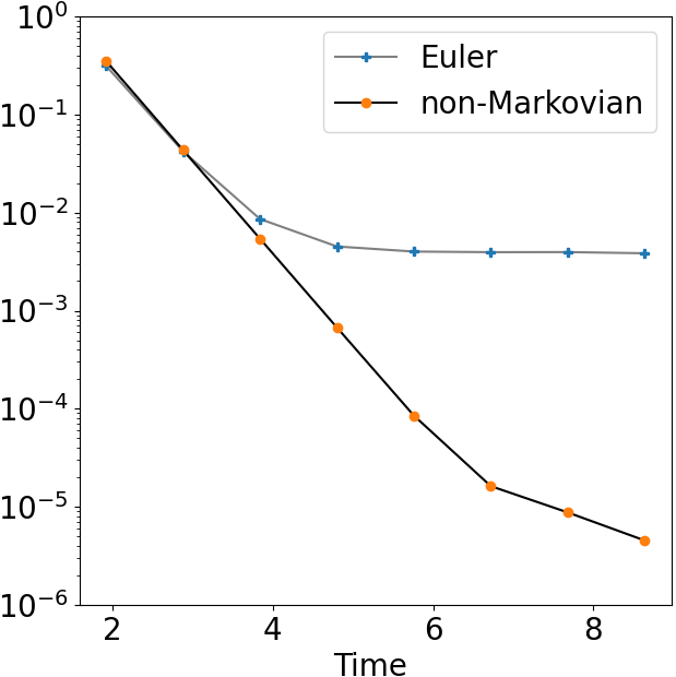
(a) Relative Entropy Error

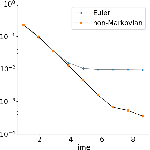
(b) $L_{2}$-Error

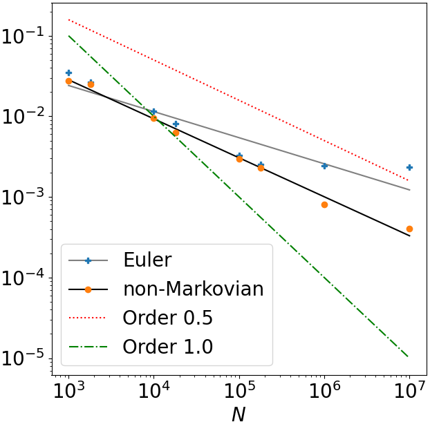
(c) PoC $L_{2}$-Error (log-scale), $T=9$

Figure 1: Simulation of the linear MV-SDE (7.1) with $\alpha=0.5,\sigma=0.8$, $N=10^{7},h=0.16$, and $X_{0}\sim\mathcal{N}(\pi,1)$ (a normal distribution with mean value $\pi$ and variance $1$). Both schemes run on the exact same samples of the initial condition and Brownian increments. (a) Entropy Error of the Euler method and non-Markovian method in log-scale over time. (b) $L_{2}$-Error of the Euler method and non-Markovian method in log-scale over time. (c) $L_{2}$-Error in particle size $N$ of the Euler method and non-Markovian method in log-scale with respect to different number of particles $N$ at $T=9$.

Figure 1 (a) and (b) show that the non-Markovian method (uniformly) outperforms the Euler method in the approximation of the stationary distribution $\mu$ in both error metrics and the difference in performance becomes more evident as time increases. This is expected from the result in Theorem 3.3, since the first order term decays exponentially as $T$ increases.

Figure 1 (c) shows (for a fixed timestep $h=0.04$) that the PoC $L_{2}$-Error of the non-Markovian method decays consistently as $N$ increases with a rate of approximately $0.5$ (the expected strong PoC $\mathcal{O}(1/\sqrt{N})$ rate). The error of the Euler method plateaus for $N>10^{5}$ as the error from the time-discretization dominates the particle error; see also Table 2 below for more information.

$\alpha$	$\sigma$	$a$	$b$	$N_{\textrm{bins}}$	timestep	Entropy Error		$L_{2}$-error
						Euler	NM	Euler	NM
$0.5$	$0.8$	$-1.8$	$1.8$	$72$	$0.04$	2.33E-04	4.71E-06	2.37E-03	3.56E-04
					0.16	3.84E-03	4.33E-06	9.47E-03	3.37E-04
					0.24	9.26E-03	4.40E-06	1.47E-02	3.25E-04
					0.48	4.31E-02	3.25E-06	3.18E-02	2.92E-04
$0.3$	$1.5$	$-3.0$	$3.0$	$120$	$0.04$	1.84E-04	7.85E-06	1.44E-03	3.81E-04
					0.16	2.98E-03	5.94E-06	5.88E-03	2.82E-04
					0.24	6.84E-03	6.07E-06	9.00E-03	3.19E-04
					0.48	3.08E-02	5.72E-06	1.95E-02	3.09E-04

Table 1: Simulation results for MV-SDE (7.1) with $N=10^{7},T=8.64$ and different choices of parameters using the non-Markovian (NM) Euler and standard Euler method, respectively. (As for Fig. 1: $X_{0}\sim\mathcal{N}(\pi,1)$ and both schemes run on the exact same samples of the initial condition and Brownian increments.)

Table 1 shows that the non-Markovian method has a significantly better approximation accuracy compared to the Euler method under different choices of timesteps and model parameters. The Euler method produces larger errors as the timestep increases and the non-Markovian method yields stable results across all choices for the timestep.

The results in Table 2 show (at fixed timestep $h=0.04$) the entropy error and the $L_{2}$-Error of the non-Markovian method decaying as the number of particles $N$ increases. However, the error of the Euler method remains stable for $N>10^{5}$ (i.e., there is a plateau). Due to computational limitations, we are not able to show results beyond $N>10^{7}$. The terminal time $T=8.64$ is chosen for convenience only (due to the smaller timestep $h=0.04$).

$\alpha$	$\sigma$	$a$	$b$	$N_{\textrm{bins}}$	$N$	Entropy Error		$L_{2}$-Error
						Euler	NM	Euler	NM
$0.5$	$0.8$	$-1.8$	$1.8$	$72$	$10^{3}$	-	-	2.89E-02	3.28E-02
					$10^{4}$	-	-	1.01E-02	1.04E-02
					$10^{5}$	8.21E-04	4.83E-04	4.29E-03	3.10E-03
					$10^{6}$	2.74E-04	4.66E-05	2.31E-03	1.26E-03
					$10^{7}$	2.33E-04	4.71E-06	2.37E-03	3.56E-04

Table 2: Simulation results for MV-SDE (7.1) with $h=0.04$ and $T=8.64$ for increasing numbers of particles $N$. (As for Fig. 1: $X_{0}\sim\mathcal{N}(\pi,1)$ and both schemes run on the exact same samples of the initial condition and Brownian increments.)

Appendix A Appendix

A.1 Proof of Proposition 2.1

Proof of Proposition 2.1.

Assumption H.1 is sufficient to guarantee the existence of the unique stationary distribution; see [13] (under their Assumption (A’)). The uniform PoC result follows from [42, Theorem 1.2]. This addresses the proposition’s last two statements.

The system’s wellposedness (as an SDE in $\mathbb{R}^{N}$) follows [42]. For completeness, we present a short proof for the moment stability of the IPS, highlighting that the constant $K$ appearing in the RHS of the inequality is independent of $t$ and $N$.

Let $p\geq 2$. Performing similar calculations as in [20, Appendix A] and applying Gronwall’s inequality, we deduce that there exists some positive constant $K$ independent of $N,t\geq 0$, such that for any $i\neq j$

$$\mathbb{E}[\,|X^{i,N}_{t}-X^{j,N}_{t}|^{p}]\leq K<\infty.$$ (A.1)

Employing Itô’s formula, we deduce for any $t\geq 0$ , $p\geq 2$ and $\kappa\in[0,\lambda)$

$$e^{p\kappa t}|X^{i,N}_{t}|^{p}-|\xi^{i}|^{p}$$

$$\leq\int_{0}^{t}p\bigg{(}\kappa|X_{s}^{i,N}|^{2}+\big{(}X_{s}^{i,N}\big{)}\cdot\Big{(}-\nabla U(X_{s}^{i,N})-\frac{1}{N}\sum_{j=1}^{N}\nabla V(X_{s}^{i,N}-X_{s}^{j,N})\Big{)}\bigg{)}e^{p\kappa s}|X^{i,N}_{s}|^{p-2}\mathrm{d}s$$

$$\quad+\sigma^{2}\frac{p(p-1)}{2}\int_{0}^{t}e^{p\kappa s}|X_{s}^{i,N}|^{p-2}\mathrm{d}s+\sigma p\int_{0}^{t}e^{p\kappa s}|X_{s}^{i,N}|^{p-2}X_{s}^{i,N}\mathrm{d}W_{s}^{i}.$$

Taking expectations on both sides, using the inequality: for $q\in\{1,2\}$

$$a^{p-q}b^{q}\leq\frac{p-q}{p}\varepsilon a^{p}+\frac{q}{p\varepsilon^{(p-q)/q}}b^{p},\qquad\textrm{for any $\varepsilon>0$ and $a,b>0$},$$

assumption H.1 and (A.1) yields

$$\mathbb{E} \left[e^{p\kappa t}|X^{i,N}_{t}|^{p}\right]-\mathbb{E}\left[|\xi^{i}|^{p}\right]$$

$$\leq p\int_{0}^{t}(\kappa-\lambda)\mathbb{E}\left[e^{p\kappa s}|X^{i,N}_{s}|^{p}\right]\mathrm{d}s$$

$$\qquad\qquad+\int_{0}^{t}e^{p\kappa s}\Big{(}\frac{K}{N}\sum_{j=1}^{N}\mathbb{E}\Big{[}|X^{i,N}_{s}|^{p-1}~{}|X^{i,N}_{s}-X^{j,N}_{s}|\Big{]}\Big{)}\mathrm{d}s+K\int_{0}^{t}e^{p\kappa s}\mathbb{E}\left[|X_{s}^{i,N}|^{p-2}\right]\mathrm{d}s$$

$$\leq p\int_{0}^{t}(\kappa-\lambda+\varepsilon)\mathbb{E}\left[e^{\kappa ps}|X^{i,N}_{s}|^{p}\right]\mathrm{d}s+K\int_{0}^{t}e^{p\kappa s}\mathrm{d}s\leq Ke^{p\kappa t},$$

for some positive constant $K$ and $\varepsilon>0$ arbitrarily small. ∎

We provide the following auxiliary results:

Proposition A.1.

Let the assumptions and set up of Proposition 2.1 hold and let the IPS be given as in (2.4). Then there exists $K\geq 0$, independent of $t,s$ and $N$, such that for any $s\geq t\geq 0,~{}s-t<1$

$$\max_{i\in\{1,\ldots,N\}}\mathbb{E}\Big{[}\big{|}X_{s}^{i,N}-X_{t}^{i,N}\big{|}^{2}\Big{]}\leq K(s-t).$$

Proof.

By Itô’s formula and an application of the Cauchy–Schwarz and Jensen inequalities, we have that for any $s\geq t\geq 0,~{}(s-t)<1$, $i\in\{1,\dots,N\}$,

$$\mathbb{E}\Big{[} \big{|}X_{s}^{i,N}-X_{t}^{i,N}\big{|}^{2}\Big{]}=\mathbb{E}\bigg{[}\bigg{|}\int_{t}^{s}-\nabla U(X_{u}^{i,N})-\frac{1}{N}\sum_{j=1}^{N}\nabla V(X_{u}^{i,N}-X_{u}^{j,N})\mathrm{d}u+\sigma\int_{t}^{s}\mathrm{d}W_{u}^{i}\bigg{|}^{2}\bigg{]}$$

$$\leq K(s-t)\int_{t}^{s}\mathbb{E}\Big{[}\big{|}\nabla U(X_{u}^{i,N})\big{|}^{2}\Big{]}+\frac{1}{N}\sum_{j=1}^{N}\mathbb{E}\Big{[}\big{|}\nabla V(X_{u}^{i,N}-X_{u}^{j,N})\big{|}^{2}\Big{]}\mathrm{d}u+K(s-t)$$

$$\leq K(s-t)\Big{(}1+\int_{t}^{s}\mathbb{E}\Big{[}\big{|}X_{u}^{i,N}\big{|}^{2}\Big{]}+\frac{1}{N}\sum_{j=1}^{N}\mathbb{E}\Big{[}\big{|}X_{u}^{j,N}\big{|}^{2}\Big{]}\mathrm{d}u\Big{)}\leq K(s-t),$$

where we used Proposition 2.1 in the last estimate. ∎

A.2 Proof of Proposition 2.2

For clarity, we prove each of the proposition’s statements separately. The main argument requires care as an analysis by cases is needed, but within each case the estimation procedure is standard.

Proof of Proposition 2.2 – Statement (1): Moment estimates.

For the scheme defined in (2.6), we introduce the following notations for any $m\in\{0,\ldots,M\}$,

$$b_{m}^{i,N,h}\coloneqq-\nabla U(X^{i,N,h}_{t_{m}})-\frac{1}{N}\sum_{j=1}^{N}\nabla V(X_{t_{m}}^{i,N,h}-X_{t_{m}}^{j,N,h}),\quad\Delta\overline{W}_{m}^{i,N,h}\coloneqq\frac{\Delta W_{m}^{i}+\Delta W_{m+1}^{i}}{2}.$$ (A.2)

Assumption H.1 implies that

$$\big{(}X_{t_{m}}^{i,N,h}-X_{t_{m}}^{j,N,h}\big{)}\cdot \big{(}~{}b_{m}^{i,N,h}-b_{m}^{j,N,h}\big{)}\leq-\lambda\big{|}X_{t_{m}}^{i,N,h}-X_{t_{m}}^{j,N,h}\big{|}^{2},$$

$$\big{|}~{}b_{m}^{i,N,h}-b_{m}^{j,N,h}\big{|}^{2} \leq 2\big{|}\nabla U(X^{i,N,h}_{t_{m}})-\nabla U(X^{j,N,h}_{t_{m}})\big{|}^{2}$$

$$\quad+\frac{2}{N}\sum_{k=1}^{N}\big{|}\nabla V(X_{t_{m}}^{i,N,h}-X_{t_{m}}^{k,N,h})-\nabla V(X_{t_{m}}^{j,N,h}-X_{t_{m}}^{k,N,h})\big{|}^{2}$$

$$\leq 2(\lambda^{2}+K_{V}^{2})|X_{t_{m}}^{i,N,h}-X_{t_{m}}^{j,N,h}|^{2}\leq K|X_{t_{m}}^{i,N,h}-X_{t_{m}}^{j,N,h}|^{2}.$$

An inspection of the above inequalities indicates that in order to establish the $L^{p}$-moments for $X_{t_{m}}^{i,N,h}$, we need $L^{p}$-estimates on the local differences $X_{t_{m}}^{i,N,h}-X_{t_{m}}^{j,N,h}$ (a term that appears from the interaction kernel). This proof is split accordingly; Part 1 deals with the latter while Part 2 with the former.

Part 1: Moments of local differences uniformly bounded in time. We first prove that for all $i,j\in\{1,\ldots,N\}$, $m\in\{0,\ldots,M\},p\geq 2$, with $p$ an even number, that $\mathbb{E}\big{[}|X_{t_{m}}^{i,N,h}-X_{t_{m}}^{j,N,h}|^{p}\big{]}$ is uniformly bounded in time. Note that due to the nature of the scheme, $X_{t_{m}}^{i,N,h}$ is not independent of $\Delta\overline{W}_{m}^{i,N,h}$, and thus we analyze the different cases as time evolves, i.e., $m\in\{0,1,2\}$ and $m\geq 3$ below. (This same procedure will be used in Part 2 of the proof.)

Case: $m=0$. For any $i,j\in\{1,\ldots,N\}$, we have

$$\mathbb{E}\big{[}|X_{t_{0}}^{i,N,h}-X_{t_{0}}^{j,N,h}|^{p}\big{]} \leq K\mathbb{E}\big{[}|X_{t_{0}}^{i,N,h}|^{p}+|X_{t_{0}}^{j,N,h}|^{p}\big{]}=K\mathbb{E}\big{[}|\xi|^{p}\big{]}.$$ (A.3)

Case: $m=1$. We get

$$|X_{t_{1}}^{i,N,h}-X_{t_{1}}^{j,N,h}|^{2} =|X_{t_{0}}^{i,N,h}+b_{0}^{i,N,h}h-X_{t_{0}}^{j,N,h}-b_{0}^{j,N,h}h|^{2}+|\sigma\Delta\overline{W}_{0}^{i,N,h}-\sigma\Delta\overline{W}_{0}^{j,N,h}|^{2}$$

$$\quad+2\big{(}X_{t_{0}}^{i,N,h}+b_{0}^{i,N,h}h-X_{t_{0}}^{j,N,h}-b_{0}^{j,N,h}h\big{)}\cdot\big{(}\sigma\Delta\overline{W}_{0}^{i,N,h}-\sigma\Delta\overline{W}_{0}^{j,N,h}\big{)}$$

$$\leq|X_{t_{0}}^{i,N,h}-X_{t_{0}}^{j,N,h}|^{2}\big{(}1-2\lambda h+Kh^{2}\big{)}+|\sigma\Delta\overline{W}_{0}^{i,N,h}-\sigma\Delta\overline{W}_{0}^{j,N,h}|^{2}$$

$$\quad+2\big{(}X_{t_{0}}^{i,N,h}+b_{0}^{i,N,h}h-X_{t_{0}}^{j,N,h}+b_{0}^{j,N,h}h\big{)}\cdot\big{(}\sigma\Delta\overline{W}_{0}^{i,N,h}-\sigma\Delta\overline{W}_{0}^{j,N,h}\big{)}.$$

Taking the power $p/2$ and expectation on both sides, we deduce that there exist positive constants $K_{p,1}$, $K_{p,2}$, $K$, $\kappa$ (both are independent of $h,T,M$ and $N$) such that

$$\mathbb{E}\big{[}|X_{t_{1}}^{i,N,h}- X_{t_{1}}^{j,N,h}|^{p}\big{]}\leq\mathbb{E}\big{[}|X_{t_{0}}^{i,N,h}-X_{t_{0}}^{j,N,h}|^{p}\big{]}\big{(}1-2\lambda h+Kh^{2}\big{)}^{p}+h\big{(}K_{p,1}\mathbb{E}\big{[}|X_{t_{0}}^{i,N,h}-X_{t_{0}}^{j,N,h}|^{p}\big{]}+K_{p,2}\big{)}$$

$$+p\mathbb{E}\big{[}|\sigma\Delta\overline{W}_{0}^{i,N,h}-\sigma\Delta\overline{W}_{0}^{j,N,h}|^{2}\cdot|X_{t_{0}}^{i,N,h}-X_{t_{0}}^{j,N,h}|^{p-2}\big{(}1-2\lambda h+Kh^{2}\big{)}^{p-2}\big{]}$$

$$\leq(1-K_{p,1}h)\mathbb{E}\big{[}|X_{t_{0}}^{i,N,h}-X_{t_{0}}^{j,N,h}|^{p}\big{]}+~{}K_{p,2}h\big{(}1+\mathbb{E}\big{[}|\xi|^{p-2}\big{]}\big{)}$$

$$\leq K\big{(}h+\mathbb{E}\big{[}|\xi|^{p}\big{]}+\mathbb{E}\big{[}|\xi|^{p-2}\big{]}\big{)}\leq Ke^{\kappa t_{1}}\big{(}1+\mathbb{E}\big{[}|\xi|^{p}\big{]}e^{-{\kappa t_{1}}}\big{)},$$

where we also used Young’s inequality. Note that in this case (and the case $m=2$) the factor $e^{-\kappa t_{1}}$ ($e^{-\kappa t_{2}}$ for $m=2$) is only added to make it consistent with the estimates obtained for a general $m$.

Case: $m=2$. Based on the calculations above, there exist positive constants $K,{\kappa}$ (both are independent of $h,T,M$ and $N$ ) such that

$$\mathbb{E}\big{[}|X_{t_{2}}^{i,N,h}-X_{t_{2}}^{j,N,h}|^{p}\big{]} \leq Ke^{\kappa t_{2}}(1+\mathbb{E}\big{[}|\xi|^{p}\big{]}e^{-{\kappa}t_{2}}).$$ (A.4)

Note that below we will show that the constant on the right-hand side will not blow up as $m$ increases.

Case: $m\geq 3$. More generally, for $m\geq 3$, we have

$$|X_{t_{m}}^{i,N,h}-X_{t_{m}}^{j,N,h}|^{2} \leq\big{(}1-2\lambda h+Kh^{2}\big{)}|X_{t_{m-1}}^{i,N,h}-X_{t_{m-1}}^{j,N,h}|^{2}+\sigma^{2}|\Delta\overline{W}_{m-1}^{i,N,h}-\Delta\overline{W}_{m-1}^{j,N,h}|^{2}$$ (A.5)

$$\quad+2\big{(}X_{t_{m-1}}^{i,N,h}+b_{m-1}^{i,N,h}h-X_{t_{m-1}}^{j,N,h}+b_{m-1}^{j,N,h}h\big{)}\cdot\big{(}\sigma\Delta\overline{W}_{m-1}^{i,N,h}-\sigma\Delta\overline{W}_{m-1}^{j,N,h}\big{)}.$$

Since for $m\geq 3$, $X_{t_{m-1}}^{i,N,h}$ is not independent of $\Delta\overline{W}_{m-1}^{i,N,h}$, we further expand $X_{t_{m-1}}^{\cdot,N,h}$ to get

$$\big{(} X_{t_{m-1}}^{i,N,h}+b_{m-1}^{i,N,h}h-X_{t_{m-1}}^{j,N,h}+b_{m-1}^{j,N,h}h\big{)}\cdot\big{(}\sigma\Delta\overline{W}_{m-1}^{i,N,h}-\sigma\Delta\overline{W}_{m-1}^{j,N,h}\big{)}$$

$$\leq\big{(}X_{t_{m-2}}^{i,N,h}-X_{t_{m-2}}^{j,N,h}+b_{m-2}^{i,N,h}h-b_{m-2}^{j,N,h}h+\sigma\Delta\overline{W}_{m-2}^{i,N,h}-\sigma\Delta\overline{W}_{m-2}^{j,N,h}\big{)}\cdot\big{(}\sigma\Delta\overline{W}_{m-1}^{i,N,h}-\sigma\Delta\overline{W}_{m-1}^{j,N,h}\big{)}$$

$$\quad+Kh\big{|}X_{t_{m-1}}^{i,N,h}-X_{t_{m-1}}^{j,N,h}\big{|}\big{|}\sigma\Delta\overline{W}_{m-1}^{i,N,h}-\sigma\Delta\overline{W}_{m-1}^{j,N,h}\big{|}.$$

Define the following local quantities: for all $i,j\in\{1,\ldots,N\}$

$$G_{m,1}^{i,j} =\big{(}1-2\lambda h+Kh^{2}\big{)}|X_{t_{m-1}}^{i,N,h}-X_{t_{m-1}}^{j,N,h}|^{2},\quad G_{m,2}^{i,j}=\sigma^{2}|\Delta\overline{W}_{m-1}^{i,N,h}-\Delta\overline{W}_{m-1}^{j,N,h}|^{2}$$

$$G_{m,3}^{i,j} =2\big{(}X_{t_{m-2}}^{i,N,h}-X_{t_{m-2}}^{j,N,h}+\sigma\Delta\overline{W}_{m-2}^{i,N,h}-\sigma\Delta\overline{W}_{m-2}^{j,N,h}\big{)}\cdot\big{(}\sigma\Delta\overline{W}_{m-1}^{i,N,h}-\sigma\Delta\overline{W}_{m-1}^{j,N,h}\big{)},$$

$$G_{m,4}^{i,j} =2\big{(}b_{m-2}^{i,N,h}h-b_{m-2}^{j,N,h}h\big{)}\cdot\big{(}\sigma\Delta\overline{W}_{m-1}^{i,N,h}-\sigma\Delta\overline{W}_{m-1}^{j,N,h}\big{)}$$

$$G_{m,5}^{i,j} =2Kh\big{|}X_{t_{m-1}}^{i,N,h}-X_{t_{m-1}}^{j,N,h}\big{|}\big{|}\sigma\Delta\overline{W}_{m-1}^{i,N,h}-\sigma\Delta\overline{W}_{m-1}^{j,N,h}\big{|}.$$

Using these local quantities, we can express the estimate (A.5) as follows:

$$|X_{t_{m}}^{i,N,h}-X_{t_{m}}^{j,N,h}|^{2} \leq\big{(}G_{m,1}^{i,j}+G_{m,2}^{i,j}+G_{m,3}^{i,j}+G_{m,4}^{i,j}+G_{m,5}^{i,j}\big{)}.$$

Now, taking the power of $p/2$ and expectations on both sides, in combination with Young’s inequality, we have for some positive constants $K_{p,1},K_{p,2},K$ ( both are independent of $h,T,M$ and $N$) such that

$$\mathbb{E}\Big{[} \big{(}G_{m,1}^{i,j}+G_{m,2}^{i,j}+G_{m,3}^{i,j}+G_{m,4}^{i,j}+G_{m,5}^{i,j}\big{)}^{p/2}\Big{]}=\sum_{l=0}^{p/2}\binom{p/2}{l}\mathbb{E}\Big{[}(G_{m,1}^{i,j})^{p/2-l}(G_{m,2}^{i,j}+G_{m,3}^{i,j}+G_{m,4}^{i,j}+G_{m,5}^{i,j})^{l}\Big{]}$$

$$\leq\mathbb{E}\big{[}|G_{m,1}^{i,j}|^{p/2}\big{]}+p\mathbb{E}\Big{[}|G_{m,1}^{i,j}|^{p/2-1}(G_{m,2}^{i,j}+G_{m,3}^{i,j}+G_{m,4}^{i,j}+G_{m,5}^{i,j})+|G_{m,1}^{i,j}|^{p/2-2}|G_{m,3}^{i,j}|^{2}\Big{]}$$ (A.6)

$$\quad+h^{3/2}\Big{(}K_{p,1}\mathbb{E}\big{[}\big{|}X_{t_{m-1}}^{i,N,h}-X_{t_{m-1}}^{j,N,h}\big{|}^{p}\big{]}+K_{p,2}\mathbb{E}\big{[}\big{|}X_{t_{m-2}}^{i,N,h}-X_{t_{m-2}}^{j,N,h}\big{|}^{p}\big{]}+K\Big{)},$$

where we used the fact that

$$\mathbb{E}\Big{[}(G_{m,1}^{i,j} )^{p/2-2}(G_{m,2}^{i,j}+G_{m,3}^{i,j}+G_{m,4}^{i,j}+G_{m,5}^{i,j})^{2}\Big{]}$$

$$\leq\mathbb{E}\Big{[}|G_{m,1}^{i,j}|^{p/2-2}|G_{m,3}^{i,j}|^{2}\Big{]}+h^{3/2}\Big{(}K\mathbb{E}\big{[}\big{|}X_{t_{m-1}}^{i,N,h}-X_{t_{m-1}}^{j,N,h}\big{|}^{p}\big{]}+K\mathbb{E}\big{[}\big{|}X_{t_{m-2}}^{i,N,h}-X_{t_{m-2}}^{j,N,h}\big{|}^{p}\big{]}+K\Big{)}.$$

We now further estimate the terms in (A.6) :

$$\mathbb{E}\big{[}(G_{m,1}^{i,j})^{p/2-1}G_{m,5}^{i,j}\big{]}$$

$$\leq Kh\mathbb{E}\left[\big{|}X_{t_{m-2}}^{i,N,h}-X_{t_{m-2}}^{j,N,h}+b_{m-2}^{i,N,h}h-b_{m-2}^{j,N,h}h+\sigma\Delta\overline{W}_{m-2}^{i,N,h}-\sigma\Delta\overline{W}_{m-2}^{j,N,h}\big{|}^{p-1}\big{|}\sigma\Delta\overline{W}_{m-1}^{i,N,h}-\sigma\Delta\overline{W}_{m-1}^{j,N,h}\big{|}\right]$$

$$\leq Kh\mathbb{E}\big{[}\big{|}X_{t_{m-2}}^{i,N,h}-X_{t_{m-2}}^{j,N,h}\big{|}^{p-1}\big{|}\sigma\Delta\overline{W}_{m-1}^{i,N,h}-\sigma\Delta\overline{W}_{m-1}^{j,N,h}\big{|}\big{]}+Kh^{3/2}\mathbb{E}\big{[}\big{|}X_{t_{m-2}}^{i,N,h}-X_{t_{m-2}}^{j,N,h}\big{|}^{p-1}\big{]}+Kh^{3/2}$$

$$\leq Kh^{3/2}\mathbb{E}\big{[}\big{|}X_{t_{m-2}}^{i,N,h}-X_{t_{m-2}}^{j,N,h}\big{|}^{p-1}\big{]}+Kh^{3/2}.$$

Also, note that we have the bound

$$\mathbb{E}\big{[}(G_{m,1}^{i,j})^{p/2}\big{]} \leq(1-Kh)\mathbb{E}\big{[}\big{|}X_{t_{m-1}}^{i,N,h}-X_{t_{m-1}}^{j,N,h}\big{|}^{p}\big{]}.$$

In the following, $\varepsilon>0$ (arbitrarily small) and $K>0$ (both are independent of $h,T,M$ and $N$) will denote positive constants appearing due to the application of Young’s inequality. In addition recall that $X_{t_{m-2}}^{\cdot,N,h}$ is independent of $W_{m-1}^{\cdot,N,h}$. Consequently, we derive

$$\mathbb{E}\big{[} (G_{m,1}^{i,j})^{p/2-1}G_{m,2}^{i,j}\big{]}\leq(1-Kh)\mathbb{E}\big{[}\big{|}X_{t_{m-1}}^{i,N,h}-X_{t_{m-1}}^{j,N,h}\big{|}^{p-2}\sigma^{2}|\Delta\overline{W}_{m-1}^{i,N,h}-\Delta\overline{W}_{m-1}^{j,N,h}|^{2}\big{]}$$

$$\leq(1-Kh)\mathbb{E}\big{[}(K+\varepsilon\big{|}X_{t_{m-1}}^{i,N,h}-X_{t_{m-1}}^{j,N,h}\big{|}^{p})\sigma^{2}|\Delta\overline{W}_{m-1}^{i,N,h}-\Delta\overline{W}_{m-1}^{j,N,h}|^{2}\big{]}$$

$$\leq Kh+\varepsilon\mathbb{E}\big{[}\big{|}X_{t_{m-2}}^{i,N,h}-X_{t_{m-2}}^{j,N,h}+b_{m-2}^{i,N,h}h-b_{m-2}^{j,N,h}h+\sigma\Delta\overline{W}_{m-2}^{i,N,h}-\sigma\Delta\overline{W}_{m-2}^{j,N,h}\big{|}^{p}\sigma^{2}|\Delta\overline{W}_{m-1}^{i,N,h}-\Delta\overline{W}_{m-1}^{j,N,h}|^{2}\big{]}$$

$$\leq Kh+\varepsilon\mathbb{E}\big{[}\big{|}X_{t_{m-2}}^{i,N,h}-X_{t_{m-2}}^{j,N,h}\big{|}^{p}\sigma^{2}|\Delta\overline{W}_{m-1}^{i,N,h}-\Delta\overline{W}_{m-1}^{j,N,h}|^{2}\big{]}+Kh^{3/2}$$

$$\quad+K\mathbb{E}\big{[}\big{|}b_{m-2}^{i,N,h}h-b_{m-2}^{i,N,h}h\big{|}^{p}\sigma^{2}|\Delta\overline{W}_{m-1}^{i,N,h}-\Delta\overline{W}_{m-1}^{j,N,h}|^{2}\big{]}$$

$$\quad+K\mathbb{E}\big{[}\big{|}\sigma\Delta\overline{W}_{m-2}^{i,N,h}-\sigma\Delta\overline{W}_{m-2}^{j,N,h}\big{|}^{p}\sigma^{2}|\Delta\overline{W}_{m-1}^{i,N,h}-\Delta\overline{W}_{m-1}^{j,N,h}|^{2}\big{]}\leq Kh+\varepsilon h\mathbb{E}\big{[}\big{|}X_{t_{m-2}}^{i,N,h}-X_{t_{m-2}}^{j,N,h}\big{|}^{p}\big{]}.$$

Similarly, we have

$$\mathbb{E}\big{[} (G_{m,1}^{i,j})^{p/2-1}(G_{m,3}^{i,j}+G_{m,4}^{i,j})\big{]}\leq Kh+\varepsilon h\mathbb{E}\big{[}\big{|}X_{t_{m-1}}^{i,N,h}-X_{t_{m-1}}^{j,N,h}\big{|}^{p}\big{]}$$

$$\quad+2(1-Kh)\mathbb{E}\big{[}\big{|}X_{t_{m-1}}^{i,N,h}-X_{t_{m-1}}^{j,N,h}\big{|}^{p-2}\big{(}X_{t_{m-1}}^{i,N,h}-X_{t_{m-1}}^{j,N,h}\big{)}\cdot\big{(}\sigma\Delta\overline{W}_{m-1}^{i,N,h}-\sigma\Delta\overline{W}_{m-1}^{j,N,h}\big{)}\big{]}$$

$$\leq K\mathbb{E}\Big{[}\big{|}\sigma\Delta\overline{W}_{m-2}^{i,N,h}-\sigma\Delta\overline{W}_{m-2}^{j,N,h}\big{|}^{p-1}\big{(}X_{t_{m-1}}^{i,N,h}-X_{t_{m-1}}^{j,N,h}\big{)}\cdot\big{(}\sigma\Delta\overline{W}_{m-1}^{i,N,h}-\sigma\Delta\overline{W}_{m-1}^{j,N,h}\big{)}\Big{]}$$

$$\quad+K\mathbb{E}\Big{[}\big{|}X_{t_{m-2}}^{i,N,h}-X_{t_{m-2}}^{j,N,h}\big{|}^{p-1}\big{(}\sigma\Delta\overline{W}_{m-2}^{i,N,h}-\sigma\Delta\overline{W}_{m-2}^{j,N,h}\big{)}\cdot\big{(}\sigma\Delta\overline{W}_{m-1}^{i,N,h}-\sigma\Delta\overline{W}_{m-1}^{j,N,h}\big{)}\Big{]}$$

$$\quad+K\mathbb{E}\Big{[}\big{|}b_{m-2}^{i,N,h}h-b_{m-2}^{i,N,h}h\big{|}^{p-1}\big{(}\sigma\Delta\overline{W}_{m-2}^{i,N,h}-\sigma\Delta\overline{W}_{m-2}^{j,N,h}\big{)}\cdot\big{(}\sigma\Delta\overline{W}_{m-1}^{i,N,h}-\sigma\Delta\overline{W}_{m-1}^{j,N,h}\big{)}\Big{]}$$

$$\quad+\varepsilon h\mathbb{E}\big{[}\big{|}X_{t_{m-1}}^{i,N,h}-X_{t_{m-1}}^{j,N,h}\big{|}^{p}\big{]}+Kh+Kh^{3/2}$$

$$\leq K\mathbb{E}\Big{[}\big{|}\sigma\Delta\overline{W}_{m-2}^{i,N,h}-\sigma\Delta\overline{W}_{m-2}^{j,N,h}\big{|}^{p-1}\big{(}X_{t_{m-3}}^{i,N,h}-X_{t_{m-3}}^{j,N,h}\big{)}\cdot\big{(}\sigma\Delta\overline{W}_{m-1}^{i,N,h}-\sigma\Delta\overline{W}_{m-1}^{j,N,h}\big{)}\Big{]}$$

$$\quad+K\mathbb{E}\Big{[}\big{|}X_{t_{m-3}}^{i,N,h}-X_{t_{m-3}}^{j,N,h}\big{|}^{p-1}\big{(}\sigma\Delta\overline{W}_{m-2}^{i,N,h}-\sigma\Delta\overline{W}_{m-2}^{j,N,h}\big{)}\cdot\big{(}\sigma\Delta\overline{W}_{m-1}^{i,N,h}-\sigma\Delta\overline{W}_{m-1}^{j,N,h}\big{)}\Big{]}$$

$$\quad+\varepsilon h\mathbb{E}\big{[}\big{|}X_{t_{m-1}}^{i,N,h}-X_{t_{m-1}}^{j,N,h}\big{|}^{p}\big{]}+Kh+Kh^{3/2}$$

$$\leq Kh+Kh^{3/2}+\varepsilon h\mathbb{E}\big{[}\big{|}X_{t_{m-3}}^{i,N,h}-X_{t_{m-3}}^{j,N,h}\big{|}^{p}\big{]}+\varepsilon h\mathbb{E}\big{[}\big{|}X_{t_{m-1}}^{i,N,h}-X_{t_{m-1}}^{j,N,h}\big{|}^{p}\big{]},$$

where we expanded the second term in the second inequality, used Young’s inequality and the fact that $X_{t_{m-3}}^{\cdot,N,h}$ is independent of $W_{m-2}^{\cdot,N,h}$. For the last term, we have

$$\mathbb{E} \big{[}(G_{m,1}^{i,j})^{p/2-2}|G_{m,3}^{i,j}|^{2}\big{]}$$

$$\leq K\mathbb{E}\big{[}\big{|}X_{t_{m-1}}^{i,N,h}-X_{t_{m-1}}^{j,N,h}\big{|}^{p-4}\big{(}\big{|}X_{t_{m-2}}^{i,N,h}-X_{t_{m-2}}^{j,N,h}\big{|}^{2}+\big{|}\sigma\Delta\overline{W}_{m-2}^{i,N,h}-\sigma\Delta\overline{W}_{m-2}^{j,N,h}\big{|}^{2}\big{)}$$

$$\qquad\quad\cdot\big{|}\sigma\Delta\overline{W}_{m-1}^{i,N,h}-\sigma\Delta\overline{W}_{m-1}^{j,N,h}\big{|}^{2}\big{]}$$

$$\leq K\mathbb{E}\big{[}\big{|}X_{t_{m-2}}^{i,N,h}-X_{t_{m-2}}^{j,N,h}+b_{m-2}^{i,N,h}h-b_{m-2}^{j,N,h}h+\sigma\Delta\overline{W}_{m-2}^{i,N,h}-\sigma\Delta\overline{W}_{m-2}^{j,N,h}\big{|}^{p-4}$$

$$\qquad\quad\cdot\big{(}\big{|}X_{t_{m-2}}^{i,N,h}-X_{t_{m-2}}^{j,N,h}\big{|}^{2}+\big{|}\sigma\Delta\overline{W}_{m-2}^{i,N,h}-\sigma\Delta\overline{W}_{m-2}^{j,N,h}\big{|}^{2}\big{)}\cdot\big{|}\sigma\Delta\overline{W}_{m-1}^{i,N,h}-\sigma\Delta\overline{W}_{m-1}^{j,N,h}\big{|}^{2}\big{]}$$

$$\leq Kh+\varepsilon h\mathbb{E}\big{[}\big{|}X_{t_{m-2}}^{i,N,h}-X_{t_{m-2}}^{j,N,h}\big{|}^{p}\big{]}.$$

Hence, there exist positive constants $K_{p,3},K_{p,4},K_{p,5}$ (all independent of $h,T,M$ and $N$) satisfying $K_{p,3}>2K_{p,4}$ (by carefully choosing the constants in Young’s inequality) such that

$$\mathbb{E} \big{[}|X_{t_{m}}^{i,N,h}-X_{t_{m}}^{j,N,h}|^{p}\big{]}$$

$$\leq(1-K_{p,3}h)\mathbb{E}\big{[}|X_{t_{m-1}}^{i,N,h}-X_{t_{m-1}}^{j,N,h}|^{p}\big{]}+K_{p,4}h\big{(}\mathbb{E}\big{[}|X_{t_{m-2}}^{i,N,h}-X_{t_{m-2}}^{j,N,h}|^{p}\big{]}+\mathbb{E}\big{[}|X_{t_{m-3}}^{i,N,h}-X_{t_{m-3}}^{j,N,h}|^{p}\big{]}\big{)}+K_{p,5}h$$

$$\leq K+Ke^{2\kappa}(1+\mathbb{E}\big{[}|\xi|^{p}\big{]})e^{-(K_{p,3}-2K_{p,4})t_{m}/3},$$ (A.7)

for some constant $K$ (independent of $h,T,M$ and $N$). In the last estimate, we used Lemma A.7 with $c_{1}\equiv(1-K_{p,3}h),c_{2}\equiv K_{p,4}h,c_{3}\equiv K_{p,4}h$, $C\equiv K_{p,5}h$ and the moment bounds for the differences process at $\{t_{0},t_{1},t_{2}\}$ in (A.3) and (A.4). Note that the condition $0<c_{1}+c_{2}+c_{3}<1$ is satisfied for our choice $h\in(0,\min\{1/2\lambda,1\})$.

We conclude that there exist some positive constants $K,{\kappa}$ (both independent of $h,T,M$ and $N$), such that for all $i,j\in\{1,\ldots,N\}$, and $m\geq 0$

$$\mathbb{E} \big{[}|X_{t_{m}}^{i,N,h}-X_{t_{m}}^{j,N,h}|^{p}\big{]}\leq K\big{(}1+\mathbb{E}\big{[}|\xi|^{p}\big{]}e^{-{\kappa}t_{m}}\big{)}.$$ (A.8)

Part 2: Moments are uniformly bounded in time. Let $p\geq 2$ be given. We now prove that for all $i\in\{1,\ldots,N\},m\geq 0,$ $\mathbb{E}\big{[}|X_{t_{m}}^{i,N,h}|^{p}\big{]}$ is uniformly bounded in time. As in Part 1, we separately consider the cases $m\in\{0,1,2\}$ then $m\geq 3$.

Let $i\in\{1,\ldots,N\}$ be arbitrary and set $m=0$. Then we have by assumption on the initial data

$$\mathbb{E}\big{[}|X_{0}^{i,N,h}|^{p}\big{]}=\mathbb{E}\big{[}|\xi|^{p}\big{]}<\infty.$$

Case 1: $m=1$. Due to Assumption H.1 and Jensen’s inequality, it follows that

$$|X_{t_{1}}^{i,N,h}|^{2} =|X_{t_{0}}^{i,N,h}+b_{0}^{i,N,h}h|^{2}+|\sigma\Delta\overline{W}_{0}^{i,N,h}|^{2}+2\big{(}X_{t_{0}}^{i,N,h}+b_{0}^{i,N,h}h\big{)}\cdot\big{(}\sigma\Delta\overline{W}_{0}^{i,N,h}\big{)}$$

$$\leq(1-2\lambda h+Kh^{2})|X_{t_{0}}^{i,N,h}|^{2}+2\big{(}X_{t_{0}}^{i,N,h}+b_{0}^{i,N,h}h\big{)}\cdot\big{(}\sigma\Delta\overline{W}_{0}^{i,N,h}\big{)}+|\sigma\Delta\overline{W}_{0}^{i,N,h}|^{2}$$

$$\quad+\frac{2K_{V}h}{N}\sum_{j=1}^{N}|X_{t_{0}}^{i,N,h}-X_{t_{0}}^{j,N,h}||X_{t_{0}}^{i,N,h}|+\frac{K_{V}^{2}h^{2}}{N}\sum_{j=1}^{N}|X_{t_{0}}^{i,N,h}-X_{t_{0}}^{j,N,h}|^{2}.$$

Raising to the power $p/2$ and taking the expectation on both sides above, an application of (A.8), Jensen’s inequality and Young’s inequality shows that there exist positive constants $K_{p,6},\kappa$ (both independent of $h,T,M$ and $N$) such that

$$\mathbb{E}\big{[}|X_{t_{1}}^{i,N,h}|^{p}\big{]} \leq e^{\kappa t_{1}}K_{p,6}\big{(}1+\mathbb{E}\big{[}|\xi|^{p}\big{]}e^{-{\kappa}t_{1}}\big{)}.$$

Case 2: $m=2$. There exist positive constants $K_{p,6},\kappa$ (both are independent of $h,T,M$ and $N$) such that

$$\mathbb{E}\big{[}|X_{t_{2}}^{i,N,h}|^{p}\big{]} \leq e^{\kappa t_{2}}K_{p,6}\big{(}1+\mathbb{E}\big{[}|\xi|^{p}\big{]}e^{-{\kappa}t_{2}}\big{)}.$$

We will show that the constant on the right-hand side does not blow up as $m$ increases.

Case 3: $m\geq 3$. We have

$$|X_{t_{m}}^{i,N,h}|^{2} =|X_{t_{m-1}}^{i,N,h}+b_{m-1}^{i,N,h}h|^{2}+\sigma^{2}|\Delta\overline{W}_{m-1}^{i,N,h}|^{2}+2\big{(}X_{t_{m-1}}^{i,N,h}+b_{m-1}^{i,N,h}h\big{)}\cdot\big{(}\Delta\overline{W}_{m-1}^{i,N,h}\big{)}$$

$$\leq(1-2\lambda h+Kh^{2})|X_{t_{m-1}}^{i,N,h}|^{2}+\sigma^{2}|\Delta\overline{W}_{m-1}^{i,N,h}|^{2}+2\big{(}X_{t_{m-1}}^{i,N,h}+b_{m-1}^{i,N,h}h\big{)}\cdot\big{(}\Delta\overline{W}_{m-1}^{i,N,h}\big{)}$$

$$\quad+\frac{2K_{V}h}{N}\sum_{j=1}^{N}|X_{t_{m-1}}^{i,N,h}-X_{t_{m-1}}^{j,N,h}||X_{t_{0}}^{i,N,h}|+\frac{K_{V}^{2}h^{2}}{N}\sum_{j=1}^{N}|X_{t_{m-1}}^{i,N,h}-X_{t_{m-1}}^{j,N,h}|^{2}.$$

Since for $m\geq 3$, $X_{t_{m-1}}^{i,N,h}$ is not independent of $\Delta\overline{W}_{m-1}^{i,N,h}$, we further expand $X_{t_{m-1}}^{i,N,h}$ and estimate

$$\big{(}X_{t_{m-1}}^{i,N,h}+b_{m-1}^{i,N,h}h\big{)}\cdot\big{(}\Delta\overline{W}_{m-1}^{i,N,h}\big{)}\leq h|b_{m-1}^{i,N,h}||\Delta\overline{W}_{m-1}^{i,N,h}|+\big{(}X_{t_{m-2}}^{i,N,h}+b_{m-2}^{i,N,h}h+\Delta\overline{W}_{m-2}^{i,N,h}\big{)}\cdot\big{(}\Delta\overline{W}_{m-1}^{i,N,h}\big{)}.$$

Note that $X_{t_{m-2}}^{\cdot,N,h}$ is independent of $W_{m-1}^{\cdot,N,h}$. Similar to the analysis of the first part, we define the following local quantities: for all $i\in\{1,\ldots,N\}$ ,

$$G_{m,1}^{i}=(1-2\lambda h+Kh^{2})|X_{t_{m-1}}^{i,N,h}|^{2},$$

$$G_{m,2}^{i}=\sigma^{2}|\Delta\overline{W}_{m-1}^{i,N,h}|^{2},$$

$$G_{m,3}^{i}=2\big{(}X_{t_{m-2}}^{i,N,h}+b_{m-2}^{i,N,h}h+\Delta\overline{W}_{m-2}^{i,N,h}\big{)}\cdot\big{(}\Delta\overline{W}_{m-1}^{i,N,h}\big{)},$$

$$G_{m,4}^{i}=2h|b_{m-1}^{i,N,h}||\Delta\overline{W}_{m-1}^{i,N,h}|,$$

$$G_{m,5}^{i}=\frac{2K_{V}h}{N}\sum_{j=1}^{N}|X_{t_{m-1}}^{i,N,h}-X_{t_{m-1}}^{j,N,h}||X_{t_{m-1}}^{i,N,h}|+\frac{K_{V}^{2}h^{2}}{N}\sum_{j=1}^{N}|X_{t_{m-1}}^{i,N,h}-X_{t_{m-1}}^{j,N,h}|^{2},$$

and note that

$$|X_{t_{m}}^{i,N,h}|^{2} \leq\big{(}G_{m,1}^{i}+G_{m,2}^{i}+G_{m,3}^{i}+G_{m,4}^{i}+G_{m,5}^{i}\big{)}.$$

Raising to the power $p/2$ and taking the expectation on both sides, we have

$$\mathbb{E}\Big{[} \big{(}G_{m,1}^{i}+G_{m,2}^{i}+G_{m,3}^{i}+G_{m,4}^{i}+G_{m,5}^{i}\big{)}^{p/2}\Big{]}$$

$$=\sum_{l=0}^{p/2}\binom{p/2}{l}\mathbb{E}\Big{[}(G_{m,1}^{i})^{p/2-l}(G_{m,2}^{i}+G_{m,3}^{i}+G_{m,4}^{i}+G_{m,5}^{i})^{l}\Big{]}$$

$$\leq\mathbb{E}\big{[}|G_{m,1}^{i}|^{p/2}\big{]}+p\mathbb{E}\Big{[}(G_{m,1}^{i})^{p/2-1}(G_{m,2}^{i}+G_{m,3}^{i}+G_{m,4}^{i}+G_{m,5}^{i})+|G_{m,1}^{i}|^{p/2-2}|G_{m,3}^{i}|^{2}\Big{]}$$

$$\quad+h^{3/2}\Big{(}K_{p,1}\mathbb{E}\big{[}\big{|}X_{t_{m-1}}^{i,N,h}\big{|}^{p}\big{]}+K_{p,2}\mathbb{E}\big{[}\big{|}X_{t_{m-2}}^{i,N,h}\big{|}^{p}\big{]}+K\Big{)}.$$

Using (A.7), we obtain the following estimate:

$$\mathbb{E}\big{[} (G_{m,1}^{i})^{p/2-1}G_{m,5}^{i}\big{]}$$

$$\leq K\mathbb{E}\bigg{[}\big{|}X_{t_{m-1}}^{i,N,h}\big{|}^{p-2}\Big{(}\frac{2K_{V}h}{N}\sum_{j=1}^{N}|X_{t_{m-1}}^{i,N,h}-X_{t_{m-1}}^{j,N,h}||X_{t_{m-1}}^{i,N,h}|+\frac{K_{V}^{2}h^{2}}{N}\sum_{j=1}^{N}|X_{t_{m-1}}^{i,N,h}-X_{t_{m-1}}^{j,N,h}|^{2}\Big{)}\bigg{]}$$

$$\leq h\Big{(}\varepsilon\mathbb{E}\big{[}\big{|}X_{t_{m-1}}^{i,N,h}\big{|}^{p}\big{]}+\frac{K}{N}\sum_{j=1}^{N}\mathbb{E}\big{[}\big{|}X_{t_{m-1}}^{i,N,h}-X_{t_{m-1}}^{j,N,h}\big{|}^{p}\big{]}\Big{)}$$

$$\leq\varepsilon h\mathbb{E}\big{[}\big{|}X_{t_{m-1}}^{i,N,h}\big{|}^{p}\big{]}+Kh(1+\mathbb{E}\big{[}|\xi|^{p}\big{]}e^{-(K_{p,3}-2K_{p,4})t_{m}/3}).$$

The analysis of the other terms works similarly as in the proof of the first part. Hence, we conclude that there exists positive constants $K_{p,7},K_{p,8},K_{p,9}$ (both independent of $h,T,M$ and $N$) satisfying $K_{p,7}>2K_{p,8}$ and $e^{-(K_{p,3}-2K_{p,4})h}\neq 1-(K_{p,7}-2K_{p,8})h>0$ (for sufficiently small $h$), such that

$$\mathbb{E}\big{[}|X_{t_{m}}^{i,N,h}|^{p}\big{]} \leq(1-K_{p,7}h)\mathbb{E}\big{[}|X_{t_{m-1}}^{i,N,h}|^{p}\big{]}+K_{p,8}h\big{(}\mathbb{E}\big{[}|X_{t_{m-2}}^{i,N,h}|^{p}\big{]}+\mathbb{E}\big{[}|X_{t_{m-3}}^{i,N,h}|^{p}\big{]}\big{)}$$

$$\hskip 170.71652pt+K_{p,9}h\big{(}1+\mathbb{E}\big{[}|\xi|^{p}\big{]}e^{-(K_{p,3}-2K_{p,4})t_{m}}\big{)}$$

$$\leq K+K(1+\mathbb{E}\big{[}|\xi|^{p}\big{]})\big{(}e^{-(K_{p,7}-2K_{p,8})t_{m}/3}+e^{-(K_{p,3}-2K_{p,4})t_{m}/3}\big{)},$$

for some constant $K$ (independent of $h,T,M$ and $N$). In the last estimate, we used the second statement in Lemma A.7 with $c_{1}\equiv(1-K_{p,7}h),c_{2}\equiv K_{p,8}h,c_{3}\equiv K_{p,8}h$, $c_{4}=K_{p,9}\mathbb{E}\big{[}|\xi|^{p}\big{]}h$, $c_{5}=K_{p,3}-2K_{p,4}$, $C\equiv K_{p,9}h$ and the moment bounds at $\{t_{0},t_{1},t_{2}\}$. ∎

Proof of Proposition 2.2 – Statement (2): the $L^{2}$-strong error.

Consider the IPS described in (2.4) and recall the auxiliary scheme of (6.38). For all $m\in\{0,\ldots,M-1\}$ with $\hat{X}_{t_{0}}^{i,N,h}=X^{i,N}_{t_{0}}$, we define

$$\hat{X}^{i,N,h}_{t_{m+1}}=\hat{X}^{i,N,h}_{t_{m}}-\Big{(}\nabla U(\hat{X}^{i,N,h}_{t_{m}}+\frac{\sigma}{2}\Delta W_{m}^{i})+\frac{1}{N}\sum_{j=1}^{N}\nabla V(\hat{X}_{t_{m}}^{i,N,h}+\frac{\sigma}{2}\Delta W_{m}^{i}-\hat{X}_{t_{m}}^{j,N,h}-\frac{\sigma}{2}\Delta W_{m}^{j})\Big{)}h+\sigma\Delta W_{m}^{i},$$

where $t_{m}:=mh$, $T:=Mh$, and $\Delta W_{m}^{i}=W^{i}_{t_{m}}-W^{i}_{t_{m-1}}$. Recall that $X^{i,N,h}_{t_{m}}=\hat{X}^{i,N,h}_{t_{m}}+\sigma\Delta W_{m}^{i}/2$. We compute the difference terms:

$$\Delta_{i,m}:=X_{t_{m}}^{i,N}-\hat{X}^{i,N,h}_{t_{m+1}}$$ (A.9)

$$=X_{t_{m}}^{i,N}-\bigg{(}X_{t_{m-1}}^{i,N}-\Big{(}\nabla U(X_{t_{m-1}}^{i,N}+\frac{\sigma}{2}\Delta W_{m}^{i})+\frac{1}{N}\sum_{j=1}^{N}\nabla V(X_{t_{m-1}}^{i,N}+\frac{\sigma}{2}\Delta W_{m}^{i}-X_{t_{m-1}}^{j,N}-\frac{\sigma}{2}\Delta W_{m}^{j})\Big{)}h+\sigma\Delta W_{m}^{i}\bigg{)}$$

$$\quad+\bigg{(}X_{t_{m-1}}^{i,N}-\Big{(}\nabla U(X_{t_{m-1}}^{i,N}+\frac{\sigma}{2}\Delta W_{m}^{i})+\frac{1}{N}\sum_{j=1}^{N}\nabla V(X_{t_{m-1}}^{i,N}+\frac{\sigma}{2}\Delta W_{m}^{i}-X_{t_{m-1}}^{j,N}-\frac{\sigma}{2}\Delta W_{m}^{j})\Big{)}h+\sigma\Delta W_{m}^{i}\bigg{)}$$

$$\quad-\bigg{(}\hat{X}^{i,N,h}_{t_{m}}-\Big{(}\nabla U(\hat{X}^{i,N,h}_{t_{m}}+\frac{\sigma}{2}\Delta W_{m}^{i})+\frac{1}{N}\sum_{j=1}^{N}\nabla V(\hat{X}_{t_{m}}^{i,N,h}+\frac{\sigma}{2}\Delta W_{m}^{i}-\hat{X}_{t_{m}}^{j,N,h}-\frac{\sigma}{2}\Delta W_{m}^{j})\Big{)}h+\sigma\Delta W_{m}^{i}\bigg{)}$$

$$=:R^{i,1}_{t_{m}}+R^{i,2}_{t_{m}}.$$

Note that here we match $X_{t_{m}}^{i,N}$ with $\hat{X}^{i,N,h}_{t_{m+1}}$ instead of $\hat{X}^{i,N,h}_{t_{m}}$.

We estimate the above terms separately and collect all the estimates an the end. For the first term, taking squares and expectations yields

$$\mathbb{E} \big{[}|R^{i,1}_{t_{m}}|^{2}\big{]}$$

$$=\mathbb{E}\bigg{[}\Big{|}~{}X_{t_{m}}^{i,N}-\bigg{(}X_{t_{m-1}}^{i,N}-\Big{(}\nabla U(X_{t_{m-1}}^{i,N}+\frac{\sigma}{2}\Delta W_{m}^{i})$$

$$\quad\quad\quad\quad\quad+\frac{1}{N}\sum_{j=1}^{N}\nabla V(X_{t_{m-1}}^{i,N}+\frac{\sigma}{2}\Delta W_{m}^{i}-X_{t_{m-1}}^{j,N}-\frac{\sigma}{2}\Delta W_{m}^{j})\Big{)}h+\sigma\Delta W_{m}^{i}\bigg{)}~{}\Big{|}^{2}\bigg{]}$$

$$=\mathbb{E}\bigg{[}\Big{|}-\int_{t_{m-1}}^{t_{m}}~{}\Big{(}\nabla U(X_{s}^{i,N})-\nabla U(X_{t_{m-1}}^{i,N}+\frac{\sigma}{2}\Delta W_{m}^{i})$$

$$\quad\quad\quad\quad\quad+\frac{1}{N}\sum_{j=1}^{N}\nabla V(X_{s}^{i,N}-X_{s}^{j,N})-\frac{1}{N}\sum_{j=1}^{N}\nabla V(X_{t_{m-1}}^{i,N}+\frac{\sigma}{2}\Delta W_{m}^{i}-X_{t_{m-1}}^{j,N}-\frac{\sigma}{2}\Delta W_{m}^{j})\Big{)}\mathrm{d}s~{}\Big{|}^{2}\bigg{]}$$

$$\leq 2h\int_{t_{m-1}}^{t_{m}}\mathbb{E}\Big{[}\big{|}\nabla U(X_{s}^{i,N})-\nabla U(X_{t_{m-1}}^{i,N}+\frac{\sigma}{2}\Delta W_{m}^{i})\big{|}^{2}\Big{]}\mathrm{d}s$$

$$\quad+2h\int_{t_{m-1}}^{t_{m}}\frac{1}{N}\sum_{j=1}^{N}\mathbb{E}\Big{[}\big{|}\nabla V(X_{s}^{i,N}-X_{s}^{j,N})-\nabla V(X_{t_{m-1}}^{i,N}+\frac{\sigma}{2}\Delta W_{m}^{i}-X_{t_{m-1}}^{j,N}-\frac{\sigma}{2}\Delta W_{m}^{j})\big{|}^{2}~{}\mathrm{d}s\Big{]}$$

$$\leq Kh\int_{t_{m-1}}^{t_{m}}\bigg{(}\mathbb{E}\Big{[}\big{|}X_{s}^{i,N}-X_{t_{m-1}}^{i,N}\big{|}^{2}\Big{]}+\mathbb{E}\Big{[}\big{|}\frac{\sigma}{2}\Delta W_{m}^{i}\big{|}^{2}\Big{]}+\frac{1}{N}\sum_{j=1}^{N}\Big{(}\mathbb{E}\Big{[}\big{|}X_{s}^{j,N}-X_{t_{m-1}}^{j,N}\big{|}^{2}\Big{]}+\mathbb{E}\Big{[}\big{|}\frac{\sigma}{2}\Delta W_{m}^{j}\big{|}^{2}\Big{]}\Big{)}~{}\bigg{)}\mathrm{d}s$$

$$\leq Kh\int_{t_{m-1}}^{t_{m}}\Big{(}\max_{i\in\{1,\ldots,N\}}\mathbb{E}\Big{[}\big{|}X_{s}^{i,N}-X_{t_{m-1}}^{i,N}\big{|}^{2}\Big{]}+h\Big{)}\mathrm{d}s~{}\leq Kh^{2},$$

where we used Jensen’s inequality, the Lipschitz continuity of the potentials and Proposition 2.1. Next, we consider the second term $R^{i,2}_{t_{m}}$. Taking squares and expectations, we have that

$$\mathbb{E} \big{[}|R^{i,2}_{t_{m}}|^{2}\big{]}$$

$$= \mathbb{E}\bigg{[}\bigg{|}~{}\Big{(}X_{t_{m-1}}^{i,N}-\Big{(}\nabla U(X_{t_{m-1}}^{i,N}+\frac{\sigma}{2}\Delta W_{m}^{i})+\frac{1}{N}\sum_{j=1}^{N}\nabla V(X_{t_{m-1}}^{i,N}+\frac{\sigma}{2}\Delta W_{m}^{i}-X_{t_{m-1}}^{j,N}-\frac{\sigma}{2}\Delta W_{m}^{j})\Big{)}h\Big{)}$$

$$\quad-\Big{(}\hat{X}^{i,N,h}_{t_{m}}-\Big{(}\nabla U(\hat{X}^{i,N,h}_{t_{m}}+\frac{\sigma}{2}\Delta W_{m}^{i})+\frac{1}{N}\sum_{j=1}^{N}\nabla V(\hat{X}_{t_{m}}^{i,N,h}+\frac{\sigma}{2}\Delta W_{m}^{i}-\hat{X}_{t_{m}}^{j,N,h}-\frac{\sigma}{2}\Delta W_{m}^{j})\Big{)}h\Big{)}~{}\bigg{|}^{2}\bigg{]}$$

$$\leq\mathbb{E}\Big{[}\big{|}X_{t_{m-1}}^{i,N}-\hat{X}^{i,N,h}_{t_{m}}\big{|}^{2}\Big{]}-h\mathbb{E}\Big{[}\Big{(}X_{t_{m-1}}^{i,N}-\hat{X}^{i,N,h}_{t_{m}}\Big{)}\cdot\Big{(}\nabla U(X_{t_{m-1}}^{i,N}+\frac{\sigma}{2}\Delta W_{m}^{i})-\nabla U(\hat{X}^{i,N,h}_{t_{m}}+\frac{\sigma}{2}\Delta W_{m}^{i})\Big{)}\Big{]}$$

$$\quad-\frac{h}{N}\sum_{j=1}^{N}\mathbb{E}\Big{[}\Big{(}X_{t_{m-1}}^{i,N}-\hat{X}^{i,N,h}_{t_{m}}\Big{)}\cdot\Big{(}\nabla V(X_{t_{m-1}}^{i,N}+\frac{\sigma}{2}\Delta W_{m}^{i}-X_{t_{m-1}}^{j,N}-\frac{\sigma}{2}\Delta W_{m}^{j})$$

$$\qquad\qquad\qquad\quad-\nabla V(\hat{X}_{t_{m}}^{i,N,h}+\frac{\sigma}{2}\Delta W_{m}^{i}-\hat{X}_{t_{m}}^{j,N,h}-\frac{\sigma}{2}\Delta W_{m}^{j})\Big{)}\Big{]}$$

$$\quad+2h^{2}\mathbb{E}\Big{[}\big{|}\nabla U(X_{t_{m-1}}^{i,N}+\frac{\sigma}{2}\Delta W_{m}^{i})-\nabla U(\hat{X}^{i,N,h}_{t_{m}}+\frac{\sigma}{2}\Delta W_{m}^{i})\big{|}^{2}\Big{]}$$

$$\quad+\frac{2h^{2}}{N}\sum_{j=1}^{N}\mathbb{E}\Big{[}\big{|}\nabla V(X_{t_{m-1}}^{i,N}+\frac{\sigma}{2}\Delta W_{m}^{i}-X_{t_{m-1}}^{j,N}-\frac{\sigma}{2}\Delta W_{m}^{j})$$

$$\qquad\qquad\qquad\quad-\nabla V(\hat{X}_{t_{m}}^{i,N,h}+\frac{\sigma}{2}\Delta W_{m}^{i}-\hat{X}_{t_{m}}^{j,N,h}-\frac{\sigma}{2}\Delta W_{m}^{j})\big{|}^{2}\Big{]}$$

$$\leq\mathbb{E}\Big{[}\big{|}X_{t_{m-1}}^{i,N}-\hat{X}^{i,N,h}_{t_{m}}\big{|}^{2}\Big{]}-h\mathbb{E}\Big{[}\Big{(}X_{t_{m-1}}^{i,N}-\hat{X}^{i,N,h}_{t_{m}}\Big{)}\cdot\Big{(}\nabla U(X_{t_{m-1}}^{i,N}+\frac{\sigma}{2}\Delta W_{m}^{i})-\nabla U(\hat{X}^{i,N,h}_{t_{m}}+\frac{\sigma}{2}\Delta W_{m}^{i})\Big{)}\Big{]}$$

$$\quad+Kh^{2}-\frac{h}{N}\sum_{j=1}^{N}\mathbb{E}\Big{[}\Big{(}X_{t_{m-1}}^{i,N}-\hat{X}^{i,N,h}_{t_{m}}\Big{)}$$

$$\quad\qquad\cdot\Big{(}\nabla V(X_{t_{m-1}}^{i,N}+\frac{\sigma}{2}\Delta W_{m}^{i}-X_{t_{m-1}}^{j,N}-\frac{\sigma}{2}\Delta W_{m}^{j})-\nabla V(\hat{X}_{t_{m}}^{i,N,h}+\frac{\sigma}{2}\Delta W_{m}^{i}-\hat{X}_{t_{m}}^{j,N,h}-\frac{\sigma}{2}\Delta W_{m}^{j})\Big{)}\Big{]},$$

where we used Jensen’s inequality, Propositions 2.1 and the Statement (1) in Proposition 2.2. We further estimate

$$\mathbb{E}[|R^{i,2}_{t_{m}}|^{2}]\leq(1-\lambda h)\mathbb{E}\Big{[}\big{|}X_{t_{m-1}}^{i,N}-\hat{X}^{i,N,h}_{t_{m}}\big{|}^{2}\Big{]}+Kh^{2}$$

$$\quad-\frac{h}{2N^{2}}\sum_{i,j=1}^{N}\mathbb{E}\Big{[}\Big{(}(X_{t_{m-1}}^{i,N}+\frac{\sigma}{2}\Delta W_{m}^{i}-X_{t_{m-1}}^{j,N}-\frac{\sigma}{2}\Delta W_{m}^{j})-(\hat{X}_{t_{m}}^{i,N,h}+\frac{\sigma}{2}\Delta W_{m}^{i}-\hat{X}_{t_{m}}^{j,N,h}-\frac{\sigma}{2}\Delta W_{m}^{j})\Big{)}$$

$$\qquad\quad\cdot\Big{(}\nabla V(X_{t_{m-1}}^{i,N}+\frac{\sigma}{2}\Delta W_{m}^{i}-X_{t_{m-1}}^{j,N}-\frac{\sigma}{2}\Delta W_{m}^{j})-\nabla V(\hat{X}_{t_{m}}^{i,N,h}+\frac{\sigma}{2}\Delta W_{m}^{i}-\hat{X}_{t_{m}}^{j,N,h}-\frac{\sigma}{2}\Delta W_{m}^{j})\Big{)}\Big{]}$$

$$\leq(1-\lambda h)\mathbb{E}\Big{[}\big{|}\Delta_{i,m-1}\big{|}^{2}\Big{]}+Kh^{2},$$

with $\Delta_{i,m}$ as defined in (A.9). We used the ‘symmetrization trick’ in (4.5) to handle the convolution term. Note that the positive constant $K$ is independent of $h,T,M$ and $N$. Hence for all $m\in\{1,\ldots,M-1\},~{}i\in\{1,\ldots,N\}$, there exists a positive constant $K$ such that

$$\mathbb{E}\Big{[}\big{|}\Delta_{i,m}\big{|}^{2}\Big{]} \leq(1-\lambda h)\mathbb{E}\Big{[}\big{|}\Delta_{i,m-1}\big{|}^{2}\Big{]}+Kh^{2}$$

$$=(1-\lambda h)^{m}\mathbb{E}\Big{[}\big{|}\Delta_{i,0}\big{|}^{2}\Big{]}+Kh^{2}\sum_{j=0}^{m-1}(1-\lambda h)^{j}\leq Kh+\frac{Kh}{\lambda},$$

where we used $\mathbb{E}\big{[}|\Delta_{i,0}|^{2}\big{]}\leq Kh$. Recall that $X^{i,N,h}_{t_{m}}=\hat{X}^{i,N,h}_{t_{m}}+\sigma\Delta W_{m}^{i}/2$. Using Statement (1) in Proposition 2.2 and (2.6), we further have

$$\mathbb{E}\Big{[}\big{|}X^{i,N,h}_{t_{m}}-\hat{X}^{i,N,h}_{t_{m}}\big{|}^{2}\Big{]} =\mathbb{E}\Big{[}\big{|}\frac{\sigma}{2}\Delta W_{m}^{i}\big{|}^{2}\Big{]}\leq Kh\quad\textrm{and}\quad\mathbb{E}\Big{[}\big{|}X^{i,N,h}_{t_{m+1}}-X^{i,N,h}_{t_{m}}\big{|}^{2}\Big{]}\leq Kh.$$

Collecting the last 3 estimates, we have for all $m\in\{1,\ldots,M-1\},~{}i\in\{1,\ldots,N\}$,

$$\mathbb{E}\Big{[}\big{|}X_{t_{m}}^{i,N}-X_{t_{m}}^{i,N,h}\big{|}^{2}\Big{]} =\mathbb{E}\Big{[}\big{|}\Delta_{i,m}+(\hat{X}^{i,N,h}_{t_{m+1}}-X^{i,N,h}_{t_{m+1}})+(X^{i,N,h}_{t_{m+1}}-X^{i,N,h}_{t_{m}})\big{|}^{2}\Big{]}$$

$$\leq K\Big{(}\mathbb{E}\Big{[}\big{|}\Delta_{i,m}\big{|}^{2}\Big{]}+\mathbb{E}\Big{[}\big{|}X^{i,N,h}_{t_{m+1}}-\hat{X}^{i,N,h}_{t_{m+1}}\big{|}^{2}\Big{]}+\mathbb{E}\Big{[}\big{|}X^{i,N,h}_{t_{m+1}}-X^{i,N,h}_{t_{m}}\big{|}^{2}\Big{]}\Big{)}\leq Kh.$$

As $K$ is independent of the critical quantities $M$ and $N$, maximizing over $i$ and $m$ yields the final result. ∎

A.3 Auxiliary results

The following statement is an auxiliary result on the differences of SDE starting at different times ($t$ and $s$ with $t\leq s$) at the same point $\bm{x}$ and is used in the proof of Proposition 4.3.

Lemma A.2.

Let the assumptions and setup of Proposition 4.3 hold and let $r\geq s\geq t\geq 0$, $u\geq 0$ with $s-t<1$. Let the starting positions $x_{i}\in L^{4}(\Omega,\mathbb{R})$ be $\mathcal{F}_{t}$-measurable random variables that are identically distributed over all $i\in\{1,\ldots,N\}$. Let $(\bm{X}^{t,\bm{x},N}_{s})_{s\geq t\geq 0}$ and $(\bm{X}^{s,\bm{x},N}_{r})_{r\geq s\geq 0}$ be the solutions of (3.2) starting from $\bm{x}$ at time $t$ and $s$, respectively. Then there exist some $\lambda_{2}\in(0,\min\{\lambda-2K_{V},\lambda_{1}\})$ and $K>0$ (both are independent of $s,t,N$), such that for any $i\in\{1,\dots,N\}$

$$\mathbb{E}\Big{[}\big{|}X^{t,x_{i},i,N}_{s+u}-X^{s,x_{i},i,N}_{s+u}\big{|}^{4}\Big{]}\leq K(s-t)^{2}e^{-4\lambda_{2}u}.$$

Proof.

By Itô’s formula, we have, for any $s\geq t\geq 0$, $u\geq 0$, $i\in\{1,\dots,N\}$

$$\mathbb{E}\Big{[}\big{|}X^{t,x_{i},i,N}_{s+u}-X^{s,x_{i},i,N}_{s+u}\big{|}^{4}\Big{]}$$

$$\leq\mathbb{E}\Big{[}\big{|}X^{t,x_{i},i,N}_{s}-X^{s,x_{i},i,N}_{s}\big{|}^{4}\Big{]}$$

$$\qquad-4\int_{0}^{u}\mathbb{E}\Big{[}\big{|}X^{t,x_{i},i,N}_{s+w}-X^{s,x_{i},i,N}_{s+w}\big{|}^{2}\Big{(}X^{t,x_{i},i,N}_{s+w}-X^{s,x_{i},i,N}_{s+w}\Big{)}\cdot\bigg{(}~{}\Big{(}\nabla U(X^{t,x_{i},i,N}_{s+w})-\nabla U(X^{s,x_{i},i,N}_{s+w})\Big{)}$$

$$\qquad+\Big{(}\frac{1}{N}\sum_{l=1}^{N}\nabla V(X^{t,x_{i},i,N}_{s+w}-X^{t,x_{l},l,N}_{s+w})-\nabla V(X^{s,x_{i},i,N}_{s+w}-X^{s,x_{l},l,N}_{s+w})\Big{)}\bigg{)}\Big{]}\mathrm{d}w$$

$$\leq\mathbb{E}\Big{[}\big{|}X^{t,x_{i},i,N}_{s}-X^{s,x_{i},i,N}_{s}\big{|}^{4}\Big{]}-4\Big{(}\lambda-\left(1+\frac{3}{4}\right)K_{V}\Big{)}\int_{0}^{u}\mathbb{E}\Big{[}\big{|}X^{t,x_{i},i,N}_{s+w}-X^{s,x_{i},i,N}_{s+w}\big{|}^{4}\Big{]}\mathrm{d}w$$

$$\qquad+\frac{K_{V}}{N}\sum_{l=1}^{N}\int_{0}^{u}\mathbb{E}\Big{[}\big{|}X^{t,x_{l},l,N}_{s+w}-X^{s,x_{l},l,N}_{s+w}\big{|}^{4}\Big{]}\mathrm{d}w,$$

where we used Young’s inequality along with Assumption H.1. From the proof of Proposition 4.3 (see, equation 4.24), we deduce that $\mathbb{E}\big{[}|X^{t,x_{i},i,N}_{s}-X^{s,x_{i},i,N}_{s}|^{4}\big{]}\leq K(s-t)^{2}$. Using the fact that $\lambda>2K_{V}$, we conclude the claim. ∎

The next statement concerning the second-order variation process is similar to Proposition 4.3 which is used in the proof in Lemma 6.1.

Proposition A.3.

Let the assumptions and set up of Lemma 4.2 and Proposition 4.3 hold. Then there exist some $\lambda_{4}\in(0,\min\{\lambda-2K_{V},\lambda_{3}\})$ and $K>0$ (both are independent of $h,T,M$ and $N$) such that for all $T\geq s\geq t\geq 0$ (with $s-t<1$) and $i\in\{1,\dots,N\}$

$$\mathbb{E}\Big{[}|X^{t,x_{i},i,N}_{T,x_{i},x_{i}}-X^{s,x_{i},i,N}_{T,x_{i},x_{i}}|^{2}\Big{]} \leq K(s-t)e^{-{2\lambda_{4}}(T-s)},$$

$$\sum_{i,j,k=1,i\neq j\neq k}^{N}\mathbb{E}\Big{[}|X^{t,x_{i},i,N}_{T,x_{j},x_{k}}-X^{s,x_{i},i,N}_{T,x_{j},x_{k}}|^{2}\Big{]} \leq\frac{K(s-t)}{N}e^{-2\lambda_{4}(T-s)},$$

and

$$\sum_{i,k=1,i\neq k}^{N}\mathbb{E}\Big{[}|X^{t,x_{i},i,N}_{T,x_{k},x_{k}}-X^{s,x_{i},i,N}_{T,x_{k},x_{k}}|^{2}+|X^{t,x_{i},i,N}_{T,x_{i},x_{k}}-X^{s,x_{i},i,N}_{T,x_{i},x_{k}}|^{2}+|X^{t,x_{i},i,N}_{T,x_{k},x_{i}} -X^{s,x_{i},i,N}_{T,x_{k},x_{i}}|^{2}\Big{]}$$

$$\leq K(s-t)e^{-2\lambda_{4}(T-s)}.$$

Proof.

This proof is a combination of the methods used to prove Proposition 4.3 and Lemma 4.4 and we streamline the presentation. For any $i,j,k\in\{1,\ldots,N\}$, we have that

$$| X^{t,x_{i},i,N}_{T,x_{j},x_{k}}-X^{s,x_{i},i,N}_{T,x_{j},x_{k}}|^{2}=|X^{t,x_{i},i,N}_{s,x_{j},x_{k}}-X^{s,x_{i},i,N}_{s,x_{j},x_{k}}|^{2}$$

$$\quad\quad-2\int_{0}^{T-s}\Big{(}X^{t,x_{i},i,N}_{s+u,x_{j}}-X^{s,x_{i},i,N}_{s+u,x_{j}}\Big{)}\cdot\Big{(}\nabla^{2}U(X^{t,x_{i},i,N}_{s+u})X^{t,x_{i},i,N}_{s+u,x_{j},x_{k}}-\nabla^{2}U(X^{s,x_{i},i,N}_{s+u})X^{s,x_{i},i,N}_{s+u,x_{j},x_{k}}\Big{)}\mathrm{d}u$$

$$\quad\quad-2\int_{0}^{T}\Big{(}X^{t,x_{i},i,N}_{s+u,x_{j},x_{k}}-X^{s,x_{i},i,N}_{s+u,x_{j},x_{k}}\Big{)}\cdot\Big{(}\frac{1}{N}\sum_{l=1}^{N}\nabla^{2}V(X^{t,x_{i},i,N}_{s+u}-X^{t,x_{l},l,N}_{s+u})(X^{t,x_{i},i,N}_{{s+u},x_{j},x_{k}}-X^{t,x_{l},l,N}_{{s+u},x_{j},x_{k}})$$

$$\quad\quad\quad\qquad\qquad-\frac{1}{N}\sum_{l=1}^{N}\nabla^{2}V(X^{s,x_{i},i,N}_{s+u}-X^{s,x_{l},l,N}_{s+u})(X^{s,x_{i},i,N}_{{s+u},x_{j},x_{k}}-X^{s,x_{l},l,N}_{{s+u},x_{j},x_{k}})\Big{)}\mathrm{d}u$$

$$\quad\quad-2\int_{0}^{T-s}\Big{(}X^{t,x_{i},i,N}_{s+u,x_{j},x_{k}}-X^{s,x_{i},i,N}_{s+u,x_{j},x_{k}}\Big{)}\cdot\Big{(}\sum_{l=1}^{N}\sum_{l^{\prime}=1}^{N}\partial^{2}_{x_{l},x_{l^{\prime}}}B_{i}(\bm{X}_{u}^{t,\bm{x},N})X^{t,x_{l},l,N}_{s+u,x_{j}}X^{t,x_{l^{\prime}},l^{\prime},N}_{s+u,x_{k}}$$

$$\quad\qquad\qquad\quad\quad-\sum_{l=1}^{N}\sum_{l^{\prime}=1}^{N}\partial^{2}_{x_{l},x_{l^{\prime}}}B_{i}(\bm{X}_{u}^{s,\bm{x},N})X^{s,x_{l},l,N}_{s+u,x_{j}}X^{s,x_{l^{\prime}},l^{\prime},N}_{s+u,x_{k}}\Big{)}~{}\mathrm{d}u.$$

The remaining steps are similar to those in the proof of Lemma 4.4 and Proposition 4.3 and we therefore omit a detailed analysis. ∎

The next statement is a classical result on the stability of SDEs with respect their initial condition.

Lemma A.4.

Let Assumption H.1 hold (with $\lambda>0$ denoting the convexity parameter) and let $p\geq 2$ be given. Let $(\bm{X}^{N}_{t})_{t\geq 0}$, and $(\bm{Y}^{N}_{t})_{t\geq 0}$ be generated from (2.4) with i.i.d. initial states $X^{i,N}_{0}\sim\mu,Y^{i,N}_{0}\sim\nu\in\mathcal{P}_{p}(\mathbb{R})$, where $\bm{X}^{N}_{0}=(X^{1,N}_{0},\ldots,X^{N,N}_{0})$ and $\bm{Y}^{N}_{0}=(Y^{1,N}_{0},\ldots,Y^{N,N}_{0})$. Then for any $i\in\{1,\ldots,N\}$, $t\geq 0$, we have

$$\mathbb{E}\Big{[}\big{|}X^{i,N}_{t}-Y^{i,N}_{t}\big{|}^{2}\Big{]}\leq e^{-2\lambda t}\mathbb{E}\Big{[}\,\big{|}X^{i,N}_{0}-Y^{i,N}_{0}\big{|}^{2}\Big{]}.$$ (A.10)

Furthermore, if $\bm{Y}^{N}_{0}\sim\mu^{N,*}$, the stationary distribution of (2.4) (given in Proposition 2.1), we have

$$\mathbb{E}\Big{[}\big{|}X^{i,N}_{t}-Y^{i,N}_{0}\big{|}^{2}\Big{]}=\mathbb{E}\Big{[}\big{|}X^{i,N}_{t}-Y^{i,N}_{t}\big{|}^{2}\Big{]}\leq e^{-2\lambda t}\mathbb{E}\Big{[}\big{|}X^{i,N}_{0}-Y^{i,N}_{0}\big{|}^{2}\Big{]}.$$ (A.11)

Proof.

This result is classical and we present only a sketch of its proof. By Itô’s formula, we have

$$\mathbb{E}\Big{[}\big{|}X^{i,N}_{t}-Y^{i,N}_{t}\big{|}^{2}\Big{]}$$

$$\leq\mathbb{E}\Big{[}\big{|}X^{i,N}_{0}-Y^{i,N}_{0}\big{|}^{2}\Big{]}-2\int_{0}^{t}\mathbb{E}\Big{[}\Big{(}X^{i,N}_{s}-Y^{i,N}_{s}\Big{)}\cdot\Big{(}\nabla U(X^{i,N}_{s})-\nabla U(Y^{i,N}_{s})\Big{)}\Big{]}\mathrm{d}s$$

$$\qquad-2\int_{0}^{t}\mathbb{E}\Big{[}\Big{(}X^{i,N}_{s}-Y^{i,N}_{s}\Big{)}\cdot\Big{(}\frac{1}{N}\sum_{l=1}^{N}\nabla V(X^{i,N}_{s}-X^{l,N}_{s})-\nabla V(Y^{i,N}_{s}-Y^{l,N}_{s})\Big{)}\Big{]}\mathrm{d}s$$

$$\leq\mathbb{E}\Big{[}\big{|}X^{i,N}_{0}-Y^{i,N}_{0}\big{|}^{2}\Big{]}-2\lambda\int_{0}^{t}\mathbb{E}\Big{[}\big{|}X^{i,N}_{s}-Y^{i,N}_{s}\big{|}^{2}\Big{]}\mathrm{d}s$$

$$\quad-\frac{1}{2N^{2}}\sum_{i=1}^{N}\sum_{l=1}^{N}\int_{0}^{t}\mathbb{E}\Big{[}\Big{(}(X^{i,N}_{s}-X^{l,N}_{s})-(Y^{i,N}_{s}-Y^{l,N}_{s})\Big{)}\cdot\Big{(}\nabla V(X^{i,N}_{s}-X^{l,N}_{s})-\nabla V(Y^{i,N}_{s}-Y^{l,N}_{s})\Big{)}\Big{]}\mathrm{d}u$$

$$\leq\mathbb{E}\Big{[}\big{|}X^{i,N}_{0}-Y^{i,N}_{0}\big{|}^{2}\Big{]}-2\lambda\int_{0}^{t}\mathbb{E}\Big{[}\big{|}X^{i,N}_{s}-Y^{i,N}_{s}\big{|}^{2}\Big{]}\mathrm{d}s,$$

where we used Assumption H.1. This estimate allows to deduce the first result (A.10).

The second result follows since $\bm{Y}^{N}_{0}\sim\mu^{N,*}$ (and thus $\bm{Y}_{t}^{N}\sim\mu^{N,*}$ for any $t\geq 0$) and the one-dimensional marginal distributions of $\mu^{N,*}$ are identical. ∎

Lemma A.5.

Let the assumptions and set up of Proposition 2.2 hold with $\xi\in L^{p}(\Omega,\mathbb{R})$ for some given $p\geq 2$. Then for the processes defined in (6.36), (6.38) and (6.39), respectively, there exists a constant $K>0$ (independent of $h,T,M$ and $N$) such that for all $m\in\{0,\ldots,M-1\}$

$$\max_{i\in\{1,\ldots,N\}}\sup_{s\in[0,h]}\mathbb{E}\big{[}\,|X_{t_{m}+s}^{i,N,h}|^{p}\big{]}\leq K\big{(}1+\mathbb{E}\big{[}\,|\xi|^{p}\big{]}e^{-\kappa t_{m}}\big{)},$$

$$\max_{i\in\{1,\ldots,N\}}\mathbb{E}\big{[}\,|\hat{X}^{i,N,h}_{t_{m}}|^{p}\big{]}\leq K\big{(}1+\mathbb{E}\big{[}\,|\xi|^{p}\big{]}e^{-\kappa t_{m}}\big{)},$$

$${\color[rgb]{0,0,0}\max_{i\in\{1,\ldots,N\}}\sup_{s\in[0,h)}\mathbb{E}\big{[}\,|\overline{X}_{t_{m}+s}^{i,N,h}|^{p}\big{]}\leq K\big{(}1+\mathbb{E}\big{[}\,|\xi|^{p}\big{]}e^{-\kappa t_{m}}\big{)}.}$$

Proof.

Using Proposition 2.2 and taking the definition of the processes in (6.36) into account, we have for all $m\in\{0,\ldots,M-1\},~{}s\in[0,h]$ and $i\in\{1,\dots,N\}$,

$$\mathbb{E}\big{[}\,|X_{t_{m}+s}^{i,N,h}|^{p}\big{]}\leq K\Big{(}\mathbb{E}\big{[}\,|X^{i,N,h}_{t_{m}}|^{p}\big{]}+\mathbb{E}\big{[}\,|\nabla U(X^{i,N,h}_{t_{m}})|^{p}\big{]}h^{p}+\frac{1}{N}\sum_{j=1}^{N}\mathbb{E}\big{[}\,|\nabla V(X_{t_{m}}^{i,N,h}-X_{t_{m}}^{j,N,h})|^{p}\big{]}h^{p}$$

$$\quad+\mathbb{E}\big{[}\,|\Delta W_{m}^{i}|^{p}\big{]}+\mathbb{E}\big{[}\,|\Delta W_{m+1,s}^{i}|^{p}\big{]}\Big{)}$$

$$\leq K(1+h^{p})\Big{(}\mathbb{E}\big{[}\,|X^{i,N,h}_{t_{m}}|^{p}\big{]}+\mathbb{E}\big{[}\,|\nabla U(X^{i,N,h}_{t_{m}})|^{p}\big{]}+\frac{1}{N}\sum_{j=1}^{N}\mathbb{E}\big{[}\,|\nabla U(X^{j,N,h}_{t_{m}})|^{p}\big{]}+1\Big{)}$$

$$\leq K\big{(}1+\mathbb{E}\big{[}\,|\xi|^{p}\big{]}e^{-\kappa t_{m}}\big{)},$$

where we used Jensen’s inequality and the fact that $\nabla U,\nabla V$ are of linear growth (Assumption H.1).

For the second and the last estimate, recall that $X^{i,N,h}_{t_{m}}=\hat{X}^{i,N,h}_{t_{m}}+\sigma\Delta W_{m}^{i}/2$ and $\overline{X}^{i,N,h}_{t_{m-1}+s}=\hat{X}^{i,N,h}_{t_{m}}+\sigma\Delta W_{m,s}^{i}/2$. We have that for all $m\in\{1,\ldots,M-1\},~{}s\in[0,h)$ (recall $h\in(0,1)$ is sufficiently small) and $i\in\{1,\dots,N\}$, we have

$$\mathbb{E}\big{[}\,|\hat{X}_{t_{m}}^{i,N,h}|^{p}\big{]} \leq K\big{(}\mathbb{E}\big{[}\,|X^{i,N,h}_{t_{m}}|^{p}\big{]}+\mathbb{E}\big{[}\,|\Delta W_{m}^{i}|^{p}\big{]}\big{)}\leq K\big{(}1+\mathbb{E}\big{[}\,|\xi|^{p}\big{]}e^{-\kappa t_{m}}\big{)},$$

$$\mathbb{E}\big{[}\,|\hat{X}_{t_{0}}^{i,N,h}|^{p}\big{]} =\mathbb{E}\big{[}\,|X^{i,N}_{t_{0}}|^{p}\big{]}=\mathbb{E}\big{[}\,|\xi|^{p}\big{]},$$

$$\mathbb{E}\big{[}\,|\overline{X}^{i,N,h}_{t_{m-1}+s}|^{p}\big{]} \leq K\big{(}\mathbb{E}\big{[}\,|\hat{X}^{i,N,h}_{t_{m}}|^{p}\big{]}+\mathbb{E}\big{[}\,|\Delta W_{m,s}^{i}|^{p}\big{]}\big{)}$$

$$\leq K\big{(}1+\mathbb{E}\big{[}\,|\xi|^{p}\big{]}e^{-\kappa t_{m-1}}e^{-\kappa h}\big{)}$$

$$\leq K\big{(}1+\mathbb{E}\big{[}\,|\xi|^{p}\big{]}e^{-\kappa t_{m-1}}\big{)}.$$

∎

Lemma A.6.

(Gronwall’s inequality). Let $T>0$ and let $\alpha,\beta$ and $u$ be real-valued functions defined on $[0,T]$. Assume that $\alpha$ and $u$ are continuous and that the negative part of $\beta$ is integrable on every closed and bounded subinterval of $[0,T]$. If $\alpha$ is non-negative and if $u$ satisfies the integral inequality

$$u(t)\leq\beta(t)+\int_{0}^{t}\alpha(s)u(s)\mathrm{d}s,\quad\forall t\in[0,T],$$

then

$$u(t)\leq\beta(t)+\int_{0}^{t}\alpha(s)\beta(s)\exp\left(\int_{s}^{t}\alpha(r)\mathrm{d}r\right)\mathrm{d}s,\quad\forall t\in[0,T].$$

If we further have that $\beta$ is non-decreasing, then

$$u(t)\leq\beta(t)\exp\left(\int_{0}^{t}\alpha(s)\mathrm{d}s\right),\quad\forall t\in[0,T].$$

The following auxiliary result is needed in the proof of Proposition 2.2.

Lemma A.7.

Let $c_{1},c_{2},c_{3},c_{4},c_{5}>0,C>0$ be real constants with $c_{1}+c_{2}+c_{3}<1$. Let $(a_{n})_{n\in\mathbb{N}}$ be a real-valued sequence satisfying $a_{n+3}\leq c_{3}a_{n+2}+c_{2}a_{n+1}+c_{1}a_{n}+C$ with initial values $0<a_{1},a_{2},a_{3}<K$, for some constant $K>0$. Then there exist some constants $K_{1},K_{2}>0$ (both are independent of $n$) such that for all $n\geq 4$

$$a_{n}\leq K_{1}+K_{2}\max\{a_{1},a_{2},a_{3}\}e^{-(1-c_{1}-c_{2}-c_{3})n/3},$$

Moreover, if $a_{n+3}\leq c_{3}a_{n+2}+c_{2}a_{n+1}+c_{1}a_{n}+C+c_{4}e^{-c_{5}n}$ and $(c_{1}+c_{2}+c_{3})\neq e^{-c_{5}}$, then there exists constants $K_{3},K_{4}>0$ (both are independent of $n$) such that for all $n\geq 4$

$$a_{n}\leq K_{3}+K_{4}\max\{a_{1},a_{2},a_{3}\}e^{-(1-c_{1}-c_{2}-c_{3})n/3}.$$

Proof.

By the condition satisfied by the sequence $(a_{n})_{n\in\mathbb{N}}$, we deduce for any $n\geq 1$

$$a_{n+3} \leq c_{3}a_{n+2}+c_{2}a_{n+1}+c_{1}a_{n}+C\leq(c_{1}+c_{2}+c_{3})\max\{a_{n},a_{n+1},a_{n+2}\}+C,$$

$$a_{n+4} \leq c_{3}a_{n+3}+c_{2}a_{n+2}+c_{1}a_{n+1}+C\leq(c_{1}+c_{2}+c_{3})\max\{a_{n+1},a_{n+2},a_{n+3}\}+C$$

$$\leq(c_{1}+c_{2}+c_{3})\max\big{\{}a_{n+1},a_{n+2},(c_{1}+c_{2}+c_{3})\max\{a_{n},a_{n+1},a_{n+2}\}+C\big{\}}+C$$

$$\leq(c_{1}+c_{2}+c_{3})\max\{a_{n},a_{n+1},a_{n+2}\}+2C,$$

$$a_{n+5} \leq c_{3}a_{n+4}+c_{2}a_{n+3}+c_{1}a_{n+2}+C\leq(c_{1}+c_{2}+c_{3})\max\{a_{n+2},a_{n+3},a_{n+4}\}+C$$

$$\leq(c_{1}+c_{2}+c_{3})\max\{a_{n},a_{n+1},a_{n+2}\}+3C.$$ (A.12)

Hence,

$$\max\{a_{n+3},a_{n+4},a_{n+5}\} \leq(c_{1}+c_{2}+c_{3})\max\{a_{n},a_{n+1},a_{n+2}\}+3C.$$

Consequently, adding $\tfrac{3C}{(c_{1}+c_{2}+c_{3})-1}<0$ on both sides, we observe

$$\max\{a_{n+3},a_{n+4},a_{n+5}\}+\frac{3C}{(c_{1}+c_{2}+c_{3})-1} \leq(c_{1}+c_{2}+c_{3})\Big{(}\max\{a_{n},a_{n+1},a_{n+2}\}+\frac{3C}{(c_{1}+c_{2}+c_{3})-1}\Big{)}.$$

Further, we derive for $n\geq 1$

$$\max\{a_{3n+1},a_{3n+2},a_{3n+3}\}+\frac{3C}{(c_{1}+c_{2}+c_{3})-1} \leq(c_{1}+c_{2}+c_{3})^{n}\Big{(}\max\{a_{1},a_{2},a_{3}\}+\frac{3C}{(c_{1}+c_{2}+c_{3})-1}\Big{)},$$

which implies

$$\max\{a_{3n+1},a_{3n+2},a_{3n+3}\} \leq(c_{1}+c_{2}+c_{3})^{n}\max\{a_{1},a_{2},a_{3}\}+\frac{3C}{1-(c_{1}+c_{2}+c_{3})}$$

$$\leq e^{-(1-c_{1}-c_{2}-c_{3})n}\max\{a_{1},a_{2},a_{3}\}+K,$$

for some $K>0$, where we used the inequality $e^{x}\geq 1+x$, for any $x\in\mathbb{R}$ and $c_{1}+c_{2}+c_{3}<1$.

Similarly, for the second claim, using the fact that $e^{-c_{5}(n+2)}<e^{-c_{5}(n+1)}<e^{-c_{5}n}$, we derive as in (A.12):

$$\max\{a_{n+3},a_{n+4},a_{n+5}\} \leq(c_{1}+c_{2}+c_{3})\max\{a_{n},a_{n+1},a_{n+2}\}+3C+3c_{4}e^{-c_{5}n}.$$

Adding $\frac{3C}{(c_{1}+c_{2}+c_{3})-1}+\frac{3e^{-c_{5}(n+1)}}{(c_{1}+c_{2}+c_{3})-e^{-c_{5}}}$ on both sides, we observe that

$$\max\{a {}_{3n+1},a_{3n+2},a_{3n+3}\}+\frac{3C}{(c_{1}+c_{2}+c_{3})-1}+\frac{3e^{-c_{5}(n+1)}}{(c_{1}+c_{2}+c_{3})-e^{-c_{5}}}$$

$$\leq(c_{1}+c_{2}+c_{3})\Big{(}\max\{a_{3n-2},a_{3n-1},a_{3n}\}+\frac{3C}{(c_{1}+c_{2}+c_{3})-1}+\frac{3e^{-c_{5}n}}{(c_{1}+c_{2}+c_{3})-e^{-c_{5}}}\Big{)}.$$

Consequently, we have

$$\max\{a_{3n+1},a_{3n+2} ,a_{3n+3}\}+\frac{3C}{(c_{1}+c_{2}+c_{3})-1}+\frac{3e^{-c_{5}(n+1)}}{(c_{1}+c_{2}+c_{3})-e^{-c_{5}}}$$

$$\leq(c_{1}+c_{2}+c_{3})^{n}\Big{(}\max\{a_{1},a_{2},a_{3}\}+\frac{3C}{(c_{1}+c_{2}+c_{3})-1}+\frac{3e^{-c_{5}}}{(c_{1}+c_{2}+c_{3})-e^{-c_{5}}}\Big{)},$$

and therefore

$$\max\{a_{3n+1},a_{3n+2},a_{3n+3}\}$$

$$\quad\leq e^{-(1-c_{1}-c_{2}-c_{3})n}\max\{a_{1},a_{2},a_{3}\}+\frac{3C}{1-(c_{1}+c_{2}+c_{3})}+\frac{3e^{-c_{5}}}{|(c_{1}+c_{2}+c_{3})-e^{-c_{5}}|}(1-e^{-c_{5}n})$$

$$\quad\leq e^{-(1-c_{1}-c_{2}-c_{3})n}\max\{a_{1},a_{2},a_{3}\}+\tilde{K}_{2},$$

for some positive constant $\tilde{K}_{2}$. ∎

A.4 Omitted residual terms of Section 6.2

In this part, we show the exact expectation form for the residual terms $R^{2}_{t_{m}},R^{3}_{t_{m}},R^{5}_{t_{m}},R^{7}_{t_{m}}$ and $R^{8}_{t_{m}}$ in Lemma 6.2. The positive constant $K$ below is independent of $h,T,M$ and $N$ and may have a different value in each line. For the residual term $R^{2}_{t_{m}}$, we have

$$\mathbb{E}\big{[}R^{2}_{t_{m}}\big{]}=K\mathbb{E}\bigg{[}\int_{t_{m}}^{t_{m}+h}\int_{t_{m}}^{q_{1}}\int_{t_{m}}^{q_{2}}\sum_{\gamma\in\Pi_{3}^{N}}\Delta W_{m,2h}^{\gamma_{3}}\cdot\partial^{5}_{x_{\gamma_{1}},x_{\gamma_{2}},x_{\gamma_{2}},x_{\gamma_{3}},x_{\gamma_{3}}}u\Big{(}t_{m+1},\overline{\bm{X}}_{q_{3}}^{N,h})\Big{)}\mathrm{d}W^{\gamma_{1}}_{q_{3}}\ \mathrm{d}{q_{2}}\ \mathrm{d}W^{\gamma_{3}}_{q_{1}}\bigg{]}$$

$$+K\mathbb{E}\bigg{[}\int_{t_{m}}^{t_{m}+h}\int_{t_{m}}^{q_{1}}\int_{t_{m}}^{q_{2}}\sum_{\gamma\in\Pi_{3}^{N}}\Delta W_{m,2h}^{\gamma_{3}}\cdot\partial^{6}_{x_{\gamma_{1}},x_{\gamma_{1}},x_{\gamma_{2}},x_{\gamma_{2}},x_{\gamma_{3}},x_{\gamma_{3}}}u\Big{(}t_{m+1},\overline{\bm{X}}_{q_{3}}^{N,h})\Big{)}\mathrm{d}{q_{3}}\ \mathrm{d}{q_{2}}\ \mathrm{d}W^{\gamma_{3}}_{q_{1}}\bigg{]}.$$

For the residual term $R^{3}_{t_{m}}$, we have

$$\mathbb{E} \big{[}R^{3}_{t_{m}}\big{]}$$

$$= Kh\mathbb{E}\bigg{[}\int_{t_{m}}^{t_{m}+h}\int_{t_{m}}^{q_{1}}\qquad\sum_{\gamma\in\Pi_{3}^{N}}\Delta W_{m,2h}^{\gamma_{3}}\cdot\partial_{x_{\gamma_{1}}}\bigg{(}\partial_{x_{\gamma_{3}}}B_{\gamma_{2}}(\overline{\bm{X}}_{q_{2}}^{N,h})\partial^{2}_{x_{\gamma_{2}},x_{\gamma_{3}}}u(t_{m+1},\overline{\bm{X}}_{q_{2}}^{N,h})\bigg{)}\mathrm{d}W^{\gamma_{1}}_{q_{2}}\ \mathrm{d}W^{\gamma_{3}}_{q_{1}}\bigg{]}$$

$$+Kh\mathbb{E}\bigg{[}\int_{t_{m}}^{t_{m}+h}\int_{t_{m}}^{q_{1}}\qquad\sum_{\gamma\in\Pi_{3}^{N}}\Delta W_{m,2h}^{\gamma_{3}}\cdot\partial^{2}_{x_{\gamma_{1}},x_{\gamma_{1}}}\bigg{(}\partial_{x_{\gamma_{3}}}B_{\gamma_{2}}(\overline{\bm{X}}_{q_{2}}^{N,h})\partial^{2}_{x_{\gamma_{2}},x_{\gamma_{3}}}u(t_{m+1},\overline{\bm{X}}_{q_{2}}^{N,h})\bigg{)}\mathrm{d}{q_{2}}\ \mathrm{d}W^{\gamma_{3}}_{q_{1}}\bigg{]}$$

$$+Kh\mathbb{E}\bigg{[}\int_{t_{m}}^{t_{m}+h}\int_{t_{m}}^{q_{1}}\qquad\sum_{\gamma\in\Pi_{3}^{N}}\Delta W_{m,2h}^{\gamma_{3}}\cdot\partial_{x_{\gamma_{1}}}\bigg{(}B_{\gamma_{2}}(\overline{\bm{X}}_{q_{2}}^{N,h})\partial^{3}_{x_{\gamma_{2}},x_{\gamma_{3}},x_{\gamma_{3}}}u(t_{m+1},\overline{\bm{X}}_{q_{2}}^{N,h})\bigg{)}\mathrm{d}W^{\gamma_{1}}_{q_{2}}\ \mathrm{d}W^{\gamma_{3}}_{q_{1}}\bigg{]}$$

$$+Kh\mathbb{E}\bigg{[}\int_{t_{m}}^{t_{m}+h}\int_{t_{m}}^{q_{1}}\qquad\sum_{\gamma\in\Pi_{3}^{N}}\Delta W_{m,2h}^{\gamma_{3}}\cdot\partial^{2}_{x_{\gamma_{1}},x_{\gamma_{1}}}\bigg{(}B_{\gamma_{2}}(\overline{\bm{X}}_{q_{2}}^{N,h})\partial^{3}_{x_{\gamma_{2}},x_{\gamma_{3}},x_{\gamma_{3}}}u(t_{m+1},\overline{\bm{X}}_{q_{2}}^{N,h})\bigg{)}\mathrm{d}{q_{2}}\ \mathrm{d}W^{\gamma_{3}}_{q_{1}}\bigg{]}$$

$$+K\mathbb{E}\bigg{[}\int_{t_{m}}^{t_{m}+h}\int_{t_{m}}^{q_{1}}\int_{t_{m}}^{q_{2}}\qquad\sum_{\gamma\in\Pi_{5}^{N}}\bigg{(}\Delta W_{m,2h}^{\gamma_{4}}\Delta W_{m,2h}^{\gamma_{5}}\cdot\partial^{5}_{x_{\gamma_{1}},\dots,x_{\gamma_{5}}}u(t_{m+1},\overline{\bm{X}}_{q_{3}}^{N,h})~{}\mathrm{d}W^{\gamma_{1}}_{q_{3}}\ \mathrm{d}W^{\gamma_{2}}_{q_{2}}\ \mathrm{d}W^{\gamma_{3}}_{q_{1}}$$

$$\qquad\qquad\qquad+\Delta W_{m,2h}^{\gamma_{4}}\Delta W_{m,2h}^{\gamma_{5}}\cdot\partial^{6}_{x_{\gamma_{1}},x_{\gamma_{1}},x_{\gamma_{2}},x_{\gamma_{3}},x_{\gamma_{4}},x_{\gamma_{5}}}u(t_{m+1},\overline{\bm{X}}_{q_{3}}^{N,h})~{}\mathrm{d}{q_{3}}\ \mathrm{d}W^{\gamma_{2}}_{q_{2}}\ \mathrm{d}W^{\gamma_{3}}_{q_{1}}\bigg{)}~{}\bigg{]}$$

$$+K\mathbb{E}\bigg{[}\int_{t_{m}}^{t_{m}+h}\int_{t_{m}}^{q_{1}}\qquad\sum_{\gamma\in\Pi_{4}^{N}}\bigg{(}\Delta W_{m,2h}^{\gamma_{3}}\Delta W_{m,2h}^{\gamma_{4}}\cdot\partial^{5}_{x_{\gamma_{1}},x_{\gamma_{1}},x_{\gamma_{2}},x_{\gamma_{3}},x_{\gamma_{4}}}u(t_{m+1},\overline{\bm{X}}_{q_{2}}^{N,h})\mathrm{d}{q_{2}}\ \mathrm{d}W^{\gamma_{2}}_{q_{1}}$$

$$\qquad\qquad\qquad+\Delta W_{m,2h}^{\gamma_{3}}\Delta W_{m,2h}^{\gamma_{4}}\cdot\partial^{5}_{x_{\gamma_{1}},x_{\gamma_{2}},x_{\gamma_{2}},x_{\gamma_{3}},x_{\gamma_{4}}}u(t_{m+1},\overline{\bm{X}}_{q_{2}}^{N,h})\mathrm{d}W^{\gamma_{1}}_{q_{2}}\ \mathrm{d}{q_{1}}$$

$$\qquad\qquad\qquad+\Delta W_{m,2h}^{\gamma_{3}}\Delta W_{m,2h}^{\gamma_{4}}\cdot\partial^{6}_{x_{\gamma_{1}},x_{\gamma_{1}},x_{\gamma_{2}},x_{\gamma_{2}},x_{\gamma_{3}},x_{\gamma_{4}}}u(t_{m+1},\overline{\bm{X}}_{q_{2}}^{N,h})\mathrm{d}{q_{2}}\ \mathrm{d}{q_{1}}\bigg{)}~{}\bigg{]}.$$

For the residual term $R^{5}_{t_{m}}$, we have

$$\mathbb{E}\big{[} R^{5}_{t_{m}}\big{]}=\sum_{\gamma\in\Pi_{5}^{N}}\mathbb{E}\bigg{[}\int_{t_{m}}^{t_{m}+h}\partial_{x_{\gamma_{1}}}\bigg{(}\Delta W_{m,2h}^{\gamma_{2}}\Delta W_{m,2h}^{\gamma_{3}}\Delta W_{m,2h}^{\gamma_{4}}\Delta W_{m,2h}^{\gamma_{5}}\cdot{\partial^{4}_{x_{\gamma_{2}},x_{\gamma_{3}},x_{\gamma_{4}},x_{\gamma_{5}}}}u(t_{m+1},\overline{\bm{X}}_{q_{1}}^{N,h})\bigg{)}\mathrm{d}W^{\gamma_{1}}_{q_{1}}\bigg{]}$$

$$\quad+\sum_{\gamma\in\Pi_{4}^{N}}\mathbb{E}\bigg{[}\int_{t_{m}}^{t_{m}+h}\partial^{2}_{x_{\gamma_{1}},x_{\gamma_{1}}}\bigg{(}\Delta W_{m,2h}^{\gamma_{2}}\Delta W_{m,2h}^{\gamma_{3}}\Delta W_{m,2h}^{\gamma_{4}}\Delta W_{m,2h}^{\gamma_{5}}\cdot\partial^{4}_{x_{\gamma_{2}},x_{\gamma_{3}},x_{\gamma_{4}},x_{\gamma_{5}}}u(t_{m+1},\overline{\bm{X}}_{q_{1}}^{N,h})\bigg{)}\mathrm{d}{q_{1}}\bigg{]}$$

$$\quad+Kh\sum_{\gamma\in\Pi_{4}^{N}}\mathbb{E}\Big{[}B_{\gamma_{1}}({\bm{X}}_{t_{m}}^{N,h})\Delta W_{m,2h}^{\gamma_{2}}\Delta W_{m,2h}^{\gamma_{3}}\Delta W_{m,2h}^{\gamma_{4}}\cdot\partial^{4}_{x_{\gamma_{1}},x_{\gamma_{2}},x_{\gamma_{3}},x_{\gamma_{4}}}u(t_{m+1},\bm{X}_{t_{m}}^{N,h})\Big{]}$$

$$\quad+Kh^{2}\sum_{\gamma\in\Pi_{4}^{N}}\mathbb{E}\Big{[}B_{\gamma_{1}}({\bm{X}}_{t_{m}}^{N,h})B_{\gamma_{2}}({\bm{X}}_{t_{m}}^{N,h})\Delta W_{m,2h}^{\gamma_{3}}\Delta W_{m,2h}^{\gamma_{4}}\cdot\partial^{4}_{x_{\gamma_{1}},x_{\gamma_{2}},x_{\gamma_{3}},x_{\gamma_{4}}}u(t_{m+1},\bm{X}_{t_{m}}^{N,h})\Big{]}$$

$$\quad+Kh^{3}\sum_{\gamma\in\Pi_{4}^{N}}\mathbb{E}\Big{[}B_{\gamma_{1}}({\bm{X}}_{t_{m}}^{N,h})B_{\gamma_{2}}({\bm{X}}_{t_{m}}^{N,h})B_{\gamma_{3}}({\bm{X}}_{t_{m}}^{N,h})\Delta W_{m,2h}^{\gamma_{4}}\cdot\partial^{4}_{x_{\gamma_{1}},x_{\gamma_{2}},x_{\gamma_{3}},x_{\gamma_{4}}}u(t_{m+1},\bm{X}_{t_{m}}^{N,h})\Big{]}$$

$$\quad+Kh^{4}\sum_{\gamma\in\Pi_{4}^{N}}\mathbb{E}\Big{[}B_{\gamma_{1}}({\bm{X}}_{t_{m}}^{N,h})B_{\gamma_{2}}({\bm{X}}_{t_{m}}^{N,h})B_{\gamma_{3}}({\bm{X}}_{t_{m}}^{N,h})B_{\gamma_{4}}({\bm{X}}_{t_{m}}^{N,h})\cdot\partial^{4}_{x_{\gamma_{1}},x_{\gamma_{2}},x_{\gamma_{3}},x_{\gamma_{4}}}u(t_{m+1},\bm{X}_{t_{m}}^{N,h})\Big{]}.$$

For the residual term $R^{7}_{t_{m}}$, we have

$$\mathbb{E}\big{[}R^{7}_{t_{m}}\big{]}= Kh\mathbb{E}\bigg{[}\int_{t_{m}}^{t_{m}+h}\int_{t_{m}}^{q_{1}}\int_{t_{m}}^{q_{2}}\sum_{\gamma\in\Pi_{5}^{N}}\partial^{5}_{x_{\gamma_{1}},x_{\gamma_{2}},x_{\gamma_{3}},x_{\gamma_{4}},x_{\gamma_{5}}}u(t_{m+1},\overline{\bm{X}}_{q_{3}}^{N,h})\mathrm{d}W^{\gamma_{1}}_{q_{3}}\ \mathrm{d}W^{\gamma_{2}}_{q_{2}}\ \mathrm{d}W^{\gamma_{3}}_{q_{1}}\bigg{]}$$

$$+Kh\mathbb{E}\bigg{[}\int_{t_{m}}^{t_{m}+h}\int_{t_{m}}^{q_{1}}\int_{t_{m}}^{q_{2}}\sum_{\gamma\in\Pi_{5}^{N}}\partial^{6}_{x_{\gamma_{1}},x_{\gamma_{1}},x_{\gamma_{2}},x_{\gamma_{3}},x_{\gamma_{4}},,x_{\gamma_{5}}}u(t_{m+1},\overline{\bm{X}}_{q_{3}}^{N,h})\mathrm{d}{q_{3}}\ \mathrm{d}W^{\gamma_{2}}_{q_{2}}\ \mathrm{d}W^{\gamma_{3}}_{q_{1}}\bigg{]}$$

$$+Kh\mathbb{E}\bigg{[}\int_{t_{m}}^{t_{m}+h}\int_{t_{m}}^{q_{1}}\sum_{\gamma\in\Pi_{4}^{N}}\partial^{5}_{x_{\gamma_{1}},x_{\gamma_{1}},x_{\gamma_{2}},x_{\gamma_{3}},x_{\gamma_{4}}}u(t_{m+1},\overline{\bm{X}}_{q_{2}}^{N,h})\mathrm{d}{q_{2}}\ \mathrm{d}W^{\gamma_{2}}_{q_{1}}\bigg{]}$$

$$+Kh\mathbb{E}\bigg{[}\int_{t_{m}}^{t_{m}+h}\int_{t_{m}}^{q_{1}}\sum_{\gamma\in\Pi_{4}^{N}}\partial^{5}_{x_{\gamma_{1}},x_{\gamma_{2}},x_{\gamma_{2}},x_{\gamma_{3}},x_{\gamma_{4}}}u(t_{m+1},\overline{\bm{X}}_{q_{2}}^{N,h})\mathrm{d}W^{\gamma_{1}}_{q_{2}}\ \mathrm{d}{q_{1}}\bigg{]}$$

$$+Kh\mathbb{E}\bigg{[}\int_{t_{m}}^{t_{m}+h}\int_{t_{m}}^{q_{1}}\sum_{\gamma\in\Pi_{4}^{N}}\partial^{6}_{x_{\gamma_{1}},x_{\gamma_{1}},x_{\gamma_{2}},x_{\gamma_{2}},x_{\gamma_{3}},x_{\gamma_{4}}}u(t_{m+1},\overline{\bm{X}}_{q_{2}}^{N,h})\mathrm{d}{q_{2}}\ \mathrm{d}{q_{1}}\bigg{]}.$$

For the residual term $R^{8}_{t_{m}}$, we have

$$\mathbb{E}\big{[}R^{8}_{t_{m}}\big{]} =Kh^{2}\mathbb{E}\bigg{[}\int_{t_{m}}^{t_{m}+h}\sum_{\gamma\in\Pi_{3}^{N}}\partial_{x_{\gamma_{1}}}\bigg{(}B_{\gamma_{2}}(\overline{\bm{X}}_{q_{1}}^{N,h})\partial^{3}_{x_{\gamma_{2}},x_{\gamma_{3}},x_{\gamma_{3}}}u(t_{m+1},\overline{\bm{X}}_{q_{1}}^{N,h})\bigg{)}~{}\mathrm{d}W^{\gamma_{1}}_{q_{1}}\bigg{]}$$

$$\quad+Kh^{2}\mathbb{E}\bigg{[}\int_{t_{m}}^{t_{m}+h}\sum_{\gamma\in\Pi_{3}^{N}}\partial^{2}_{x_{\gamma_{1}},x_{\gamma_{1}}}\bigg{(}B_{\gamma_{2}}(\overline{\bm{X}}_{q_{1}}^{N,h})\partial^{3}_{x_{\gamma_{2}},x_{\gamma_{3}},x_{\gamma_{3}}}u(t_{m+1},\overline{\bm{X}}_{q_{1}}^{N,h})\bigg{)}~{}\mathrm{d}{q_{1}}\bigg{]}$$

$$\quad+Kh^{2}\mathbb{E}\bigg{[}\int_{t_{m}}^{t_{m}+h}\sum_{\gamma\in\Pi_{3}^{N}}\partial_{x_{\gamma_{1}}}\bigg{(}\partial_{x_{\gamma_{3}}}B_{\gamma_{2}}(\overline{\bm{X}}_{q_{1}}^{N,h})\partial^{2}_{x_{\gamma_{2}},x_{\gamma_{3}}}u(t_{m+1},\overline{\bm{X}}_{q_{1}}^{N,h})\bigg{)}~{}\mathrm{d}W^{\gamma_{1}}_{q_{1}}\bigg{]}$$

$$\quad+Kh^{2}\mathbb{E}\bigg{[}\int_{t_{m}}^{t_{m}+h}\sum_{\gamma\in\Pi_{3}^{N}}\partial^{2}_{x_{\gamma_{1}},x_{\gamma_{1}}}\bigg{(}\partial_{x_{\gamma_{3}}}B_{\gamma_{2}}(\overline{\bm{X}}_{q_{1}}^{N,h})\partial^{2}_{x_{\gamma_{2}},x_{\gamma_{3}}}u(t_{m+1},\overline{\bm{X}}_{q_{1}}^{N,h})\bigg{)}~{}\mathrm{d}{q_{1}}\bigg{]}$$

$$\quad+Kh^{2}\mathbb{E}\bigg{[}\int_{t_{m}}^{t_{m}+h}\sum_{\gamma\in\Pi_{3}^{N}}\partial^{5}_{x_{\gamma_{1}},x_{\gamma_{2}},x_{\gamma_{2}},x_{\gamma_{3}},x_{\gamma_{3}}}u(t_{m+1},\overline{\bm{X}}_{q_{1}}^{N,h})~{}\mathrm{d}W^{\gamma_{1}}_{q_{1}}\bigg{]}$$

$$\quad+Kh^{2}\mathbb{E}\bigg{[}\int_{t_{m}}^{t_{m}+h}\sum_{\gamma\in\Pi_{3}^{N}}\partial^{6}_{x_{\gamma_{1}},x_{\gamma_{1}},x_{\gamma_{2}},x_{\gamma_{2}},x_{\gamma_{3}},x_{\gamma_{3}}}u(t_{m+1},\overline{\bm{X}}_{q_{1}}^{N,h})~{}\mathrm{d}{q_{1}}\bigg{]}.$$

References

- [1] A. Agarwal, A. Amato, G. dos Reis, and S. Pagliarani. Numerical approximation of McKean-Vlasov SDEs via stochastic gradient descent. arXiv preprint arXiv:2310.13579, 2023.
- [2] F. Antonelli and A. Kohatsu-Higa. Rate of convergence of a particle method to the solution of the McKean–Vlasov equation. The Annals of Applied Probability, 12(2):423–476, 2002.
- [3] V. Bally and D. Talay. The Euler scheme for stochastic differential equations: error analysis with Malliavin calculus. Mathematics and Computers in Simulation, 38(1-3):35–41, 1995.
- [4] V. Bally and D. Talay. The law of the Euler scheme for stochastic differential equations. I. Convergence rate of the distribution function. Probability Theory and Related Fields, 104(1):43–60, 1996.
- [5] V. Bally and D. Talay. The law of the Euler scheme for stochastic differential equations. II. Convergence rate of the density. Monte Carlo Methods and Applications, 2(2):93–128, 1996.
- [6] J. Bao, C. Reisinger, P. Ren, and W. Stockinger. First-order convergence of Milstein schemes for McKean–Vlasov equations and interacting particle systems. Proceedings of the Royal Society A, 477(2245):20200258, 2021.
- [7] O. Bencheikh and B. Jourdain. Bias behaviour and antithetic sampling in mean-field particle approximations of SDEs nonlinear in the sense of McKean. ESAIM: Proceedings and Surveys, 65:219–235, 2019.
- [8] S. Biswas, C. Kumar, Neelima, G. d. Reis, and C. Reisinger. An explicit Milstein-type scheme for interacting particle systems and McKean–Vlasov SDEs with common noise and non-differentiable drift coefficients. The Annals of Applied Probability, 34(2):2326–2363, 2024.
- [9] M. Bossy and D. Talay. Convergence rate for the approximation of the limit law of weakly interacting particles: application to the Burgers equation. The Annals of Applied Probability, 6(3):818–861, 1996.
- [10] M. Bossy and D. Talay. A stochastic particle method for the McKean–Vlasov and the Burgers equation. Mathematics of Computation, 66(217):157–192, 1997.
- [11] N. Bou-Rabee and K. Schuh. Convergence of unadjusted Hamiltonian Monte Carlo for mean-field models. Electronic Journal of Probability, 28:Paper No. 91, 40, 2023.
- [12] N. Bou-Rabee and K. Schuh. Nonlinear Hamiltonian Monte Carlo & its particle approximation. arXiv preprint arXiv:2308.11491, 2023.
- [13] P. Cattiaux, A. Guillin, and F. Malrieu. Probabilistic approach for granular media equations in the non-uniformly convex case. Probability Theory and Related Fields, 140(1):19–40, 2008.
- [14] L.-P. Chaintron and A. Diez. Propagation of chaos: a review of models, methods and applications. II. applications. arXiv preprint arXiv:2106.14812, 2021.
- [15] L.-P. Chaintron and A. Diez. Propagation of chaos: a review of models, methods and applications. I. models and methods. Kinetic & Related Models, 15(6), 2022.
- [16] J.-F. Chassagneux, L. Szpruch, and A. Tse. Weak quantitative propagation of chaos via differential calculus on the space of measures. The Annals of Applied Probability, 32(3):1929–1969, 2022.
- [17] P. E. Chaudru de Raynal and C. A. Garcia Trillos. A cubature based algorithm to solve decoupled McKean–Vlasov forward-backward stochastic differential equations. Stochastic Processes and their Applications, 125(6):2206–2255, 2015.
- [18] F. Chen, Y. Lin, Z. Ren, and S. Wang. Uniform-in-time propagation of chaos for kinetic mean field Langevin dynamics. Electronic Journal of Probability, 29:Paper No. 17, 43, 2024.
- [19] F. Chen, Z. Ren, and S. Wang. Uniform-in-time propagation of chaos for mean field Langevin dynamics. arXiv preprint arXiv:2212.03050, 2022.
- [20] X. Chen and G. dos Reis. Euler simulation of interacting particle systems and McKean–Vlasov SDEs with fully super-linear growth drifts in space and interaction. IMA Journal of Numerical Analysis, 44(2):751–796, 2024.
- [21] X. Chen, G. dos Reis, and W. Stockinger. Wellposedness, exponential ergodicity and numerical approximation of fully super-linear McKean–Vlasov SDEs and associated particle systems. arXiv preprint arXiv:2302.05133, 2023.
- [22] L. Chizat and F. Bach. On the global convergence of gradient descent for over-parameterized models using optimal transport. Advances in Neural Information Processing systems, 31, 2018.
- [23] J. Claisse, G. Conforti, Z. Ren, and S. Wang. Mean field optimization problem regularized by Fisher information. arXiv preprint arXiv:2302.05938, 2023.
- [24] D. Crisan and E. McMurray. Cubature on Wiener space for McKean–Vlasov SDEs with smooth scalar interaction. The Annals of Applied Probability, 29(1):130–177, 2019.
- [25] V. De Bortoli, A. Durmus, X. Fontaine, and U. Simsekli. Quantitative propagation of chaos for SGD in wide neural networks. Advances in Neural Information Processing Systems, 33:278–288, 2020.
- [26] F. Delarue and A. Tse. Uniform in time weak propagation of chaos on the torus. arXiv preprint arXiv:2104.14973, 2021.
- [27] G. dos Reis, S. Engelhardt, and G. Smith. Simulation of McKean-Vlasov SDEs with super-linear growth. IMA Journal of Numerical Analysis, 42(1):874–922, 2022.
- [28] A. Durmus, A. Eberle, A. Guillin, and R. Zimmer. An elementary approach to uniform in time propagation of chaos. Proceedings of the American Mathematical Society, 148:12–43, 2020.
- [29] S. Eilenberg and S. M. Lane. On the groups , I. Annals of Mathematics, 58(1):55–106, 1953.
- [30] J. M. Foster, G. dos Reis, and C. Strange. High order splitting methods for SDEs satisfying a commutativity condition. SIAM Journal on Numerical Analysis, 62(1):500–532, 2024.
- [31] A. Friedman. Stochastic differential equations and applications. Vol. 1, volume Vol. 28 of Probability and Mathematical Statistics. Academic Press [Harcourt Brace Jovanovich, Publishers], New York-London, 1975.
- [32] A. Guillin and P. Monmarché. Uniform long-time and propagation of chaos estimates for mean field kinetic particles in non-convex landscapes. Journal of Statistical Physics, 185(2):Paper No. 15, 20, 2021.
- [33] A.-L. Haji-Ali, H. Hoel, and R. Tempone. A simple approach to proving the existence, uniqueness, and strong and weak convergence rates for a broad class of McKean–Vlasov equations. arXiv preprint arXiv:2101.00886, 2021.
- [34] K. Hu, Z. Ren, D. Šiška, and L. Szpruch. Mean-field Langevin dynamics and energy landscape of neural networks. Annales de l’Institut Henri Poincaré, Probabilités et Statistiques, 57(4):2043–2065, 2021.
- [35] P. E. Kloeden and E. Platen. Numerical solution of stochastic differential equations, volume 23 of Applications of Mathematics (New York). Springer-Verlag, Berlin, 1992.
- [36] A. Kohatsu-Higa and S. Ogawa. Weak rate of convergence for an Euler scheme of nonlinear SDE’s. Monte Carlo Methods and Applications, 3(4):327–345, 1997.
- [37] Y. Kook, M. S. Zhang, S. Chewi, M. A. Erdogdu, et al. Sampling from the mean-field stationary distribution. arXiv preprint arXiv:2402.07355, 2024.
- [38] D. Lacker. Hierarchies, entropy, and quantitative propagation of chaos for mean field diffusions. Probability and Mathematical Physics, 4(2):377–432, 2023.
- [39] D. Lacker and L. Le Flem. Sharp uniform-in-time propagation of chaos. Probability Theory and Related Fields, 187(1-2):443–480, 2023.
- [40] B. Leimkuhler, C. Matthews, and M. Tretyakov. On the long-time integration of stochastic gradient systems. Proceedings of the Royal Society A: Mathematical, Physical and Engineering Sciences, 470(2170):20140120, 2014.
- [41] R. Maillet. A note on the long-time behaviour of stochastic McKean–Vlasov equations with common noise. arXiv preprint arXiv:2306.16130, 2023.
- [42] F. Malrieu. Logarithmic Sobolev inequalities for some nonlinear PDE’s. Stochastic Processes and their Applications, 95(1):109–132, 2001.
- [43] S. Mei, A. Montanari, and P. Nguyen. A mean field view of the landscape of two-layer neural networks. Proceedings of the National Academy of Sciences, 115(33), 2018.
- [44] S. Méléard. Asymptotic behaviour of some interacting particle systems; McKean–Vlasov and Boltzmann models. In Probabilistic models for nonlinear partial differential equations (Montecatini Terme, 1995), volume 1627, pages 42–95. Springer, Berlin, 1996.
- [45] G. N. Milstein and M. V. Tretyakov. Stochastic numerics for mathematical physics. Scientific Computation. Springer, Cham, second edition, 2021.
- [46] R. Naito and T. Yamada. A higher order weak approximation of McKean–Vlasov type SDEs. BIT. Numerical Mathematics, 62(2):521–559, 2022.
- [47] E. Platen and N. Bruti-Liberati. Numerical solution of stochastic differential equations with jumps in finance, volume 64 of Stochastic Modelling and Applied Probability. Springer-Verlag, Berlin, 2010.
- [48] J. Sirignano and K. Spiliopoulos. Mean field analysis of deep neural networks. Mathematics of Operations Research, 47(1):120–152, 2022.
- [49] T. Suzuki, D. Wu, and A. Nitanda. Mean-field Langevin dynamics: Time-space discretization, stochastic gradient, and variance reduction. Advances in Neural Information Processing Systems, 36, 2024.
- [50] A.-S. Sznitman. Topics in propagation of chaos. In École d’Été de Probabilités de Saint-Flour XIX—1989, volume 1464 of Lecture Notes in Math., pages 165–251. Springer, Berlin, 1991.
- [51] D. Talay. Second-order discretization schemes of stochastic differential systems for the computation of the invariant law. Stochastics: An International Journal of Probability and Stochastic Processes, 29(1):13–36, 1990.
- [52] D. Talay and L. Tubaro. Expansion of the global error for numerical schemes solving stochastic differential equations. Stochastic Analysis and Applications, 8(4):483–509, 1990.
- [53] G. Vilmart. Postprocessed integrators for the high order integration of ergodic SDEs. SIAM Journal on Scientific Computing, 37(1):A201–A220, 2015.