Metric Dimension and Geodetic Set Parameterized by Vertex Cover

Abstract

For a graph $G$, a subset $S\subseteq V(G)$ is called a resolving set of $G$ if, for any two vertices $u,v\in V(G)$, there exists a vertex $w\in S$ such that $d(w,u)\neq d(w,v)$. The Metric Dimension problem takes as input a graph $G$ on $n$ vertices and a positive integer $k$, and asks whether there exists a resolving set of size at most $k$. In another metric-based graph problem, Geodetic Set, the input is a graph $G$ and an integer $k$, and the objective is to determine whether there exists a subset $S\subseteq V(G)$ of size at most $k$ such that, for any vertex $u\in V(G)$, there are two vertices $s_{1},s_{2}\in S$ such that $u$ lies on a shortest path from $s_{1}$ to $s_{2}$.

These two classical problems turn out to be intractable with respect to the natural parameter, i.e., the solution size, as well as most structural parameters, including the feedback vertex set number and pathwidth. Some of the very few existing tractable results state that they are both  with respect to the vertex cover number $\mathtt{vc}$.

More precisely, we observe that both problems admit an  algorithm running in time $2^{\mathcal{O}(\mathtt{vc}^{2})}\cdot n^{\mathcal{O}(1)}$, and a kernelization algorithm that outputs a kernel with $2^{\mathcal{O}(\mathtt{vc})}$ vertices. We prove that unless the Exponential Time Hypothesis (ETH) fails, Metric Dimension and Geodetic Set, even on graphs of bounded diameter, do not admit

• an  algorithm running in time $2^{o(\mathtt{vc}^{2})}\cdot n^{\mathcal{O}(1)}$, nor

• a kernelization algorithm that reduces the solution size and outputs a kernel with $2^{o(\mathtt{vc})}$ vertices.

The versatility of our technique enables us to apply it to both these problems.

We only know of one other problem in the literature that admits such a tight lower bound. Similarly, the list of known problems with exponential lower bounds on the number of vertices in kernelized instances is very short.

1 Introduction

In this article, we study two metric-based graph problems, one of which is defined through distances, while the other relies on shortest paths. Metric-based graph problems are ubiquitous in computer science; for example, the classical (Single-Source) Shortest Path, (Graphic) Traveling Salesperson or Steiner Tree problems fall into this category. Those are fundamental problems, often stemming from applications in network design, for which a considerable amount of algorithmic research has been done. Metric-based graph packing and covering problems, like Distance Domination [27] or Scattered Set [28], have recently gained a lot of attention. Their non-local nature leads to non-trivial algorithmic properties that differ from most graph problems with a more local nature.

We focus here on the Metric Dimension and Geodetic Set problems, which arise from network monitoring and network design, respectively. As noted in the introduction of [6] and the conclusion of [29], and recently demonstrated in [3, 19], these two metric-based graph covering problems share many algorithmic properties. They have far-reaching applications, as exemplified by, e.g., the recent work [3] where it is shown that enumerating minimal solution sets for the Metric Dimension and Geodetic Set problems in (general) graphs and split graphs, respectively, is equivalent to the enumeration of minimal transversals in hypergraphs, whose solvability in total-polynomial time is arguably the most important open problem in algorithmic enumeration. Formally, these two problems are defined as follows.

Metric Dimension Input: A graph $G$ and a positive integer $k$. Question: Does there exist $S\subseteq V(G)$ such that $|S|\leq k$ and, for any pair of vertices $u,v\in V(G)$, there exists a vertex $w\in S$ with $d(w,u)\neq d(w,v)$?

Geodetic Set Input: A graph $G$ and a positive integer $k$. Question: Does there exist $S\subseteq V(G)$ such that $|S|\leq k$ and, for any vertex $u\in V(G)$, there are two vertices $s_{1},s_{2}\in S$ such that $u$ lies on a shortest path from $s_{1}$ to $s_{2}$?

Metric Dimension dates back to the 1970s [25, 36], whereas Geodetic Set was introduced in 1993 [24]. The non-local nature of these problems has since posed interesting algorithmic challenges. Metric Dimension was first shown to be -complete in general graphs in Garey and Johnson’s book [21], and this was later extended to many restricted graph classes (see ‘Related work’ below). Geodetic Set was proven to be -complete in the seminal paper [24], and later shown to be -hard on restricted graph classes as well.

As these two problems are -hard even in very restricted cases, it is natural to ask for ways to confront this hardness. In this direction, the parameterized complexity paradigm allows for a more refined analysis of a problem’s complexity. In this setting, we associate each instance $I$ of a problem with a parameter $\ell$, and are interested in algorithms running in time $f(\ell)\cdot|I|^{\mathcal{O}(1)}$ for some computable function $f$. Parameterized problems that admit such an algorithm are called fixed-parameter tractable ( for short) with respect to the considered parameter. On the other hand, under standard complexity assumptions, parameterized problems that are hard for the complexity class [1] or [2] do not admit such algorithms. A parameter may originate from the formulation of the problem itself (called a natural parameter) or it can be a property of the input (called a structural parameter).

This approach, however, had limited success in the case of these two problems. In the seminal paper [26], Metric Dimension was proven to be [2]-hard parameterized by the solution size $k$, even in subcubic bipartite graphs. Similarly, Geodetic Set is [2]-hard parameterized by the solution size [15, 29], even on chordal bipartite graphs. These initial hardness results drove the ensuing meticulous study of the problems under structural parameterizations. We present an overview of such results in ‘Related work’ below. In this article, we focus on the vertex cover number, denoted by $\mathtt{vc}$, of the input graph and prove the following positive results.

Theorem 1.1.

Metric Dimension and Geodetic Set admit

• algorithms running in time $2^{\mathcal{O}(\mathtt{vc}^{2})}\cdot n^{\mathcal{O}(1)}$, and

• kernelization algorithms that output kernels with $2^{\mathcal{O}(\mathtt{vc})}$ vertices.

The second set of results follows from simple reduction rules, and was also observed in [26] for Metric Dimension. The first set of results builds on the second set by using a simple, but critical observation. For Metric Dimension, this also improves upon the $2^{2^{\mathcal{O}(\mathtt{vc})}}\cdot n^{\mathcal{O}(1)}$ algorithm mentioned in [26]. Our main technical contribution, however, is in proving that these results are optimal assuming the Exponential Time Hypothesis (ETH).

Theorem 1.2.

Unless the ETH fails, Metric Dimension and Geodetic Set do not admit

• algorithms running in time $2^{o(\mathtt{vc}^{2})}\cdot n^{\mathcal{O}(1)}$, nor

• kernelization algorithms that reduce the solution size and output kernels with $2^{o(\mathtt{vc})}$ vertices,

even on graphs of bounded diameter.

Both of these statements constitute a rare set of results in the existing literature. We know of only one other problem in the literature that admits a lower bound of the form $2^{o(\mathtt{vc}^{2})}\cdot n^{\mathcal{O}(1)}$ and a matching upper bound [1] - whereas such results parameterized by pathwidth are mentioned in [34] and [35]. Very recently, the authors in [7] also proved a similar result with respect to solution size. Similarly, the list of known problems with exponential lower bounds on the number of vertices in kernelized instances is very short. To the best of our knowledge, the only known results of this kind (that is, ETH-based lower bounds on the number of vertices in a kernel) are for Edge Clique Cover [13], Biclique Cover [9], Strong Metric Dimension [19], B-NCTD⁺ [8], and Locating Dominating Set [7]. For Metric Dimension, the above also improves a result of [23], which states that Metric Dimension parameterized by $k+\mathtt{vc}$ does not admit a polynomial kernel unless the polynomial hierarchy collapses to its third level. Indeed, the result of [23] does not rule out a kernel of super-polynomial or sub-exponential size.

In a recent work [19], the present set of authors proved that unless the ETH fails, Metric Dimension and Geodetic Set on graphs of bounded diameter do not admit $2^{2^{o(\mathtt{tw})}}\cdot n^{\mathcal{O}(1)}$-time algorithms, thereby establishing one of the first such results for -complete problems. Note that $n\succ\mathtt{vc}\succ\mathtt{fvs}\succ\mathtt{tw}$ and $n\succ\mathtt{vc}\succ\mathtt{td}\succ\mathtt{pw}\succ\mathtt{tw}$ in the parameter hierarchy, where $n$ is the number of vertices, $\mathtt{fvs}$ is the feedback vertex set number, $\mathtt{td}$ is the treedepth, and $\mathtt{tw}$ is the treewidth of the graph. The authors further proved that their lower bound also holds for $\mathtt{fvs}$ and $\mathtt{td}$ in the case of Metric Dimension, and for $\mathtt{td}$ in the case of Geodetic Set [19]. Note that a simple brute-force algorithm enumerating all possible candidates runs in time $2^{\mathcal{O}(n)}$ for both of these problems. Thus, the next natural question is whether such a lower bound for Metric Dimension and Geodetic Set can be extended to larger parameters, in particular $\mathtt{vc}$. Our first results answer this question in the negative. Together with the lower bounds with respect to $\mathtt{vc}$, this establishes the boundary between parameters yielding single-exponential and double-exponential running times for Metric Dimension and Geodetic Set.

Related Work.

We mention here results concerning structural parameterizations of Metric Dimension and Geodetic Set, and refer the reader to the full version of [19] for a more comprehensive overview of applications and related work regarding these two problems.

As previously mentioned, Metric Dimension is [2]-hard parameterized by the solution size $k$, even in subcubic bipartite graphs [26]. Several other parameterizations have been studied for this problem, on which we elaborate next (see also [20, Figure 1]). Through careful algorithmic design, kernelization, and/or meta-theorems, it was proven that there is an  algorithm parameterized by the feedback edge set number [18], and  algorithms parameterized by the max leaf number [17], the modular-width and the treelength plus the maximum degree [2], the treedepth and the clique-width plus the diameter [22], and the distance to cluster (co-cluster, respectively) [20]. Recently, an  algorithm parameterized by the treewidth in chordal graphs was given in [5]. On the negative side, Metric Dimension is [1]-hard parameterized by the pathwidth even on graphs of constant degree [4], para--hard parameterized by the pathwidth [32], and [1]-hard parameterized by the combined parameter feedback vertex set number plus pathwidth [20].

The parameterized complexity of Geodetic Set was first addressed in [29], in which they observed that the reduction from [15] implies that the problem is [2]-hard parameterized by the solution size (even for chordal bipartite graphs). This motivated the authors of [29] to investigate structural parameterizations of Geodetic Set. They proved the problem to be [1]-hard for the combined parameters solution size, feedback vertex set number, and pathwidth, and  for the parameters treedepth, modular-width (more generally, clique-width plus diameter), and feedback edge set number [29]. The problem was also shown to be  on chordal graphs when parameterized by the treewidth [6].

2 Preliminaries

For an integer $a$, we let $[a]=\{1,\ldots,a\}$.

Graph theory.

We use standard graph-theoretic notation and refer the reader to [14] for any undefined notation. For an undirected graph $G$, the sets $V(G)$ and $E(G)$ denote its set of vertices and edges, respectively. Two vertices $u,v\in V(G)$ are adjacent or neighbors if $(u,v)\in E(G)$. The open neighborhood of a vertex $u\in V(G)$, denoted by $N(u):=N_{G}(u)$, is the set of vertices that are neighbors of $u$. The closed neighborhood of a vertex $u\in V(G)$ is denoted by $N[u]:=N_{G}[u]:=N_{G}(u)\cup\{u\}$. For any $X\subseteq V(G)$ and $u\in V(G)$, $N_{X}(u)=N_{G}(u)\cap X$. Any two vertices $u,v\in V(G)$ are true twins if $N[u]=N[v]$, and are false twins if $N(u)=N(v)$. Observe that if $u$ and $v$ are true twins, then $(u,v)\in E(G)$, but if they are only false twins, then $(u,v)\not\in E(G)$. For a subset $S$ of $V(G)$, we say that the vertices in $S$ are true (false, respectively) twins if, for any $u,v\in S$, $u$ and $v$ are true (false, respectively) twins. The distance between two vertices $u,v\in V(G)$ in $G$, denoted by $d(u,v):=d_{G}(u,v)$, is the length of a $(u,v)$-shortest path in $G$. For a subset $S$ of $V(G)$, we define $N[S]=\bigcup_{v\in S}N[v]$ and $N(S)=N[S]\setminus S$. For a subset $S$ of $V(G)$, we denote the graph obtained by deleting $S$ from $G$ by $G-S$. We denote the subgraph of $G$ induced on the set $S$ by $G[S]$. For a graph $G$, a set $X\subseteq V(G)$ is said to be a vertex cover if $V(G)\setminus X$ is an independent set. We denote by $\mathtt{vc}(G)$ the size of a minimum vertex cover in $G$. When $G$ is clear from the context, we simply say $\mathtt{vc}$.

Metric Dimension and Geodetic Set.

A subset of vertices $S\subseteq V(G)$ resolves a pair of vertices $u,v\in V(G)$ if there exists a vertex $w\in S$ such that $d(w,u)\neq d(w,v)$. A subset of vertices $S\subseteq V(G)$ is a resolving set of $G$ if it resolves all pairs of vertices $u,v\in V(G)$. A vertex $u\in V(G)$ is distinguished by a subset of vertices $S\subseteq V(G)$ if, for any $v\in V(G)\setminus\{u\}$, there exists a vertex $w\in S$ such that $d(w,u)\neq d(w,v)$.

Let $G$ be a graph. For any (true or false) twins $u,v\in V(G)$ and any $w\in V(G)\setminus\{u,v\}$, $d(u,w)=d(v,w)$, and so, for any resolving set $S$ of $G$, $S\cap\{u,v\}\neq\emptyset$.

Proof 2.1.

As $w\in V(G)\setminus\{u,v\}$, and $u$ and $v$ are (true or false) twins, the shortest $(u,w)$- and $(v,w)$-paths contain a vertex of $N:=N(u)\setminus\{v\}=N(v)\setminus\{u\}$, and $d(u,w)=d(v,w)$. Hence, any resolving set $S$ of $G$ contains at least one of $u$ and $v$.

A subset $S\subseteq V(G)$ is a geodetic set if for every $u\in V(G)$, the following holds: there exist $s_{1},s_{2}\in S$ such that $u$ lies on a shortest path from $s_{1}$ to $s_{2}$. The following simple observation is used throughout the paper. Recall that a vertex is simplicial if its neighborhood forms a clique. Observe that any simplicial vertex $v$ does not belong to any shortest path between any pair $x,y$ of vertices (both distinct from $v$). Hence, the following observation follows:

[[10]] If a graph $G$ contains a simplicial vertex $v$, then $v$ belongs to any geodetic set of $G$. Specifically, degree-$1$ vertex $v$ belongs to any geodetic set of $G$.

Parameterized Complexity.

An instance of a parameterized problem $\Pi$ comprises an input $I$, which is an input of the classical instance of the problem, and an integer $\ell$, which is called the parameter. A problem $\Pi$ is said to be fixed-parameter tractable or in  if given an instance $(I,\ell)$ of $\Pi$, we can decide whether or not $(I,\ell)$ is a Yes-instance of $\Pi$ in time $f(\ell)\cdot|I|^{\mathcal{O}(1)}$, for some computable function $f$ whose value depends only on $\ell$.

A kernelization algorithm for $\Pi$ is a polynomial-time algorithm that takes as input an instance $(I,\ell)$ of $\Pi$ and returns an equivalent instance $(I^{\prime},\ell^{\prime})$ of $\Pi$, where $|I^{\prime}|,\ell^{\prime}\leq f(\ell)$, where $f$ is a function that depends only on the initial parameter $\ell$. If such an algorithm exists for $\Pi$, we say that $\Pi$ admits a kernel of size $f(\ell)$. If $f$ is a polynomial or exponential function of $\ell$, we say that $\Pi$ admits a polynomial or exponential kernel, respectively. If $\Pi$ is a graph problem, then $I$ contains a graph, say $G$, and $I^{\prime}$ contains a graph, say $G^{\prime}$. In this case, we say that $\Pi$ admits a kernel with $f(\ell)$ vertices if the number of vertices of $G^{\prime}$ is at most $f(\ell)$.

It is typical to describe a kernelization algorithm as a series of reduction rules. A reduction rule is a polynomial time algorithm that takes as an input an instance of a problem and outputs another (usually reduced) instance. A reduction rule said to be applicable on an instance if the output instance is different from the input instance. A reduction rule is safe if the input instance is a Yes-instance if and only if the output instance is a Yes-instance.

The Exponential Time Hypothesis roughly states that $n$-variable 3-SAT cannot be solved in time $2^{o(n)}$. For more on parameterized complexity and related terminologies, we refer the reader to the recent book by Cygan et al. [12].

3-Partitioned-3-SAT.

Our lower bound proofs consist of reductions from the 3-Partitioned-3-SAT problem. This version of 3-SAT was introduced in [31] and is defined as follows.

3-Partitioned-3-SAT Input: A formula $\psi$ in $3$-CNF form, together with a partition of the set of its variables into three disjoint sets $X^{\alpha}$, $X^{\beta}$, $X^{\gamma}$, with $|X^{\alpha}|=|X^{\beta}|=|X^{\gamma}|=n$, and such that no clause contains more than one variable from each of $X^{\alpha},X^{\beta}$, and $X^{\gamma}$. Question: Determine whether $\psi$ is satisfiable.

The authors of [31] also proved the following.

Proposition 2.2 [31, Theorem 3].

Unless the ETH fails, 3-Partitioned-3-SAT does not admit an algorithm running in time $2^{o(n)}$.

3 Metric Dimension: Lower Bounds Regarding Vertex Cover

In this section, we first prove the following theorem.

Theorem 3.1.

There is an algorithm that, given an instance $\psi$ of 3-Partitioned-3-SAT on $N$ variables, runs in time $2^{\mathcal{O}(\sqrt{N})}$, and constructs an equivalent instance $(G,k)$ of Metric Dimension such that $\mathtt{vc}(G)+k=\mathcal{O}(\sqrt{N})$ (and $|V(G)|=2^{\mathcal{O}(\sqrt{N})}$).

The above theorem, along with the arguments that are standard to prove the ETH-based lower bounds, immediately implies the following results.

Corollary 3.2.

Unless the ETH fails, Metric Dimension does not admit an algorithm running in time $2^{o(\mathtt{vc}^{2})}\cdot n^{\mathcal{O}(1)}$.

Corollary 3.3.

Unless the ETH fails, Metric Dimension does not admit a kernelization algorithm that reduces the solution size $k$ and outputs a kernel with $2^{o(k+\mathtt{vc})}$ vertices.

Proof 3.4.

(Proof assuming Theorem 3.1) For the sake of contradiction, assume that such a kernelization algorithm exists. Consider the following algorithm for $3$-SAT. Given a $3$-SAT formula on $N$ variables, it uses Theorem 3.1 to obtain an equivalent instance of $(G,k)$ such that $\mathtt{vc}(G)+k=\mathcal{O}(\sqrt{N})$ and $|V(G)|=2^{\mathcal{O}(\sqrt{N})}$. Then, it uses the assumed kernelization algorithm to construct an equivalent instance $(H,k^{\prime})$ such that $H$ has $2^{o(\mathtt{vc}(G)+k)}$ vertices and $k^{\prime}\leq k$. Finally, it uses a brute-force algorithm, running in time $|V(H)|^{\mathcal{O}(k^{\prime})}$, to determine whether the reduced instance, or equivalently the input instance of $3$-SAT, is a Yes-instance. The correctness of the algorithm follows from the correctness of the respective algorithms and our assumption. The total running time of the algorithm is $2^{\mathcal{O}(\sqrt{N})}+(|V(G)|+k)^{\mathcal{O}(1)}+|V(H)|^{\mathcal{O}(k^{\prime})}=2^{\mathcal{O}(\sqrt{N})}+(2^{\mathcal{O}(\sqrt{N})})^{\mathcal{O}(1)}+(2^{o(\sqrt{N})})^{\mathcal{O}(\sqrt{N})}=2^{o(N)}$. But this contradicts the ETH.

Before presenting the reduction, we first introduce some preliminary tools.

3.1 Preliminary Tools

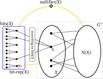
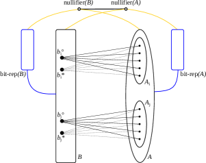
Figure 1: Set Identifying Gadget (left). The blue box represents $\textsf{bit-rep}(X)$. The yellow lines represent that all possible edges exist between $\textsf{bit-rep}(X)$ and $\textsf{nullifier}(X)$, $\textsf{nullifier}(X)$ and $N(X)$, and $y_{\star}$ and $X$. Note that $G^{\prime}$ is not necessarily restricted to the graph induced by the vertices in $X\cup N(X)$. Vertex Selector Gadget (right). For $X\in\{B,A\}$, the blue box represents $\textsf{bit-rep}(X)$, the blue link represents the connection with respect to the binary representation, and the yellow line represents that $\textsf{nullifier}(X)$ is adjacent to each vertex in the set. Dotted lines highlight absent edges.

3.1.1 Set Identifying Gadget

We redefine a gadget we introduced in [19]. Suppose that we are given a graph $G^{\prime}$ and a subset $X\subseteq V(G^{\prime})$ of its vertices. Further, suppose that we want to add a vertex set $X^{+}$ to $G^{\prime}$ in order to obtain a new graph $G$ with the following properties. We want that each vertex in $X\cup X^{+}$ will be distinguished by vertices in $X^{+}$ that must be in any resolving set $S$ of $G$, and no vertex in $X^{+}$ can resolve any “critical pair” of vertices in $V(G)$ (critical pairs will be defined in the next subsection).

The graph induced by the vertices of $X^{+}$, along with the edges connecting $X^{+}$ to $G^{\prime}$, is referred to as the Set Identifying Gadget for the set $X$ [19].

Given a graph $G^{\prime}$ and a non-empty subset $X\subseteq V(G^{\prime})$ of its vertices, to construct such a graph $G$, we add vertices and edges to $G^{\prime}$ as follows:

• The vertex set $X^{+}$ that we are aiming to add is the union of a set $\textsf{bit-rep}(X)$ and a special vertex denoted by $\textsf{nullifier}(X)$.

• First, let $X=\{x_{i}\mid i\in[|X|]\}$, and set $q:=\lceil\log(|X|+2)\rceil+1$. We select this value for $q$ to (1) uniquely represent each integer in $[|X|]$ by its bit-representation in binary (note that we start from $1$ and not $0$), (2) ensure that the only vertex whose bit-representation contains all $1$’s is $\textsf{nullifier}(X)$, and (3) reserve one spot for an additional vertex $y_{\star}$.

• For every $i\in[q]$, add three vertices $y^{a}_{i},y_{i},y^{b}_{i}$, and add the path $(y^{a}_{i},y_{i},y^{b}_{i})$.

• Add three vertices $y^{a}_{\star},y_{\star},y^{b}_{\star}$, and add the path $(y^{a}_{\star},y_{\star},y^{b}_{\star})$. Add all the edges to make $\{y_{i}\mid\ i\in[q]\}\cup\{y_{\star}\}$ into a clique. Make $y_{\star}$ adjacent to each vertex $v\in X$. We denote $\textsf{bit-rep}(X)=\{y_{i},y^{a}_{i},y^{b}_{i}\mid i\in[q]\}\cup\{y_{\star},y^{a}_{\star},y^{b}_{\star}\}$ and its subset $\textsf{bits}(X)=\{y^{a}_{i},y^{b}_{i}\mid i\in[q]\}\cup\{y^{a}_{\star},y^{b}_{\star}\}$ for convenience in a later case analysis.

• For every integer $j\in[|X|]$, let $\textsf{bin}(j)$ denote the binary representation of $j$ using $q$ bits. Connect $x_{j}$ with $y_{i}$ if the $i^{th}$ bit (going from left to right) in $\textsf{bin}(j)$ is $1$.

• Add a vertex, denoted by $\textsf{nullifier}(X)$, and make it adjacent to every vertex in $\{y_{i}\mid i\in[q]\}\cup\{y_{\star}\}$. One can think of the vertex $\textsf{nullifier}(X)$ as the only vertex whose bit-representation contains all $1$’s.

• For every vertex $u\in V(G)\setminus(X\cup X^{+})$ such that $u$ is adjacent to some vertex in $X$, add an edge between $u$ and $\textsf{nullifier}(X)$. We add this vertex to ensure that vertices in $\textsf{bit-rep}(X)$ do not resolve critical pairs in $V(G)$.

This completes the construction of $G$. The properties of $G$ are not proven yet, but just given as an intuition behind its construction. See Figure 1 for an illustration.

3.1.2 Gadget to Add Critical Pairs

Any resolving set needs to resolve all pairs of vertices in the input graph. As we will see, some pairs, which we call critical pairs, are harder to resolve than others. In fact, the non-trivial part will be to resolve all of the critical pairs.

Suppose that we need to have many critical pairs in a graph $G$, say $\langle c^{\circ}_{i},c^{\star}_{i}\rangle$ for every $i\in[m]$ for some $m\in\mathbb{N}$. Define $C:=\{c^{\circ}_{i},c^{\star}_{i}\mid i\in[m]\}$. We then add $\textsf{bit-rep}(C)$ and $\textsf{nullifier}(C)$ as mentioned above (taking $C$ as the set $X$), but the connection across $\{c^{\circ}_{i},c^{\star}_{i}\}$ and $\textsf{bit-rep}(C)$ is defined by $\textsf{bin}(i)$, i.e., connect both $c^{\circ}_{i}$ and $c^{\star}_{i}$ with the $j$-th vertex of $\textsf{bit-rep}(C)$ if the $j^{th}$ digit (going from left to right) in $\textsf{bin}(i)$ is $1$. Hence, $\textsf{bit-rep}(C)$ can resolve any pair of the form $\langle c^{\circ}_{i},c^{\star}_{\ell}\rangle$, $\langle c^{\circ}_{i},c^{\circ}_{\ell}\rangle$, or $\langle c^{\star}_{i},c^{\star}_{\ell}\rangle$ as long as $i\neq\ell$. As before, $\textsf{bit-rep}(C)$ can also resolve all pairs with one vertex in $C\cup\textsf{bit-rep}(C)\cup\{\textsf{nullifier}(C)\}$, but no critical pair of vertices. Again, when these facts will be used, they will be proven formally.

3.1.3 Vertex Selector Gadgets

Suppose that we are given a collection of sets $A_{1},A_{2},\dots,A_{q}$ of vertices in a graph $G$, and we want to ensure that any resolving set of $G$ includes at least one vertex from $A_{i}$ for every $i\in[q]$. In the following, we construct a gadget that achieves a slightly weaker objective.

• Let $A=\underset{i\in[q]}{\bigcup}A_{i}$. Add a set identifying gadget for $A$ as mentioned in Subsection 3.1.1.

• For every $i\in[q]$, add two vertices $b^{\circ}_{i}$ and $b^{\star}_{i}$. Use the gadget mentioned in Subsection 3.1.2 to make all the pairs of the form $\langle b^{\circ}_{i},b^{\star}_{i}\rangle$ critical pairs.

• For every $a\in A_{i}$, add an edge $(a,b^{\circ}_{i})$. We highlight that we do not make $a$ adjacent to $b^{\star}_{i}$ by a dotted line in Figure 1. Also, add the edges $(a,\textsf{nullifier}(B))$, $(b^{\circ}_{i},\textsf{nullifier}(A))$, $(b^{\star}_{i},\textsf{nullifier}(A))$, and $(\textsf{nullifier}(A),\textsf{nullifier}(B))$.

This completes the construction.

Note that the only vertices that can resolve a critical pair $\langle b^{\circ}_{i},b^{\star}_{i}\rangle$, apart from $b^{\circ}_{i}$ and $b^{\star}_{i}$, are the vertices in $A_{i}$. Hence, every resolving set contains at least one vertex in $\{b^{\circ}_{i},b^{\star}_{i}\}\cup A_{i}$. Again, when used, these facts will be proven formally.

3.2 Reduction

Consider an instance $\psi$ of 3-Partitioned-3-SAT with $X^{\alpha},X^{\beta},X^{\gamma}$ the partition of the variable set. By adding dummy variables in each of these sets, we can assume that $\sqrt{n}$ is an integer. From $\psi$, we construct the graph $G$ as follows. We describe the construction of $X^{\alpha}$, with the constructions for $X^{\beta}$ and $X^{\gamma}$ being analogous. We rename the variables in $X^{\alpha}$ to $x^{\alpha}_{i,j}$ for $i,j\in[\sqrt{n}]$.

• We partition the variables of $X^{\alpha}$ into buckets $X^{\alpha}_{1},X^{\alpha}_{2},\dots,X^{\alpha}_{\sqrt{n}}$ such that each bucket contains $\sqrt{n}$ many variables. Let $X^{\alpha}_{i}=\{x^{\alpha}_{i,j}\ |\ j\in[\sqrt{n}]\}$ for all $i\in[\sqrt{n}]$.

• For every $X^{\alpha}_{i}$, we construct the set $A^{\alpha}_{i}$ of $2^{\sqrt{n}}$ new vertices, $A^{\alpha}_{i}=\{a^{\alpha}_{i,\ell}\mid\ell\in[2^{\sqrt{n}}]\}$. Each vertex in $A^{\alpha}_{i}$ corresponds to a certain possible assignment of variables in $X^{\alpha}_{i}$. Let $A^{\alpha}$ be the collection of all the vertices added in the above step. Formally, $A^{\alpha}=\{a^{\alpha}_{i,\ell}\in A_{i}|\ i\in[\sqrt{n}]\text{ and }\ell\in[2^{\sqrt{n}}]\}$. We add a set identifying gadget as mentioned in Subsection 3.1.1 in order to resolve every pair of vertices in $A^{\alpha}$.

• For every $X^{\alpha}_{i}$, we construct a pair $\langle b^{\alpha,\circ}_{i},b^{\alpha,\star}_{i}\rangle$ of vertices. Then, we add a gadget to make the pairs $\{\langle b^{\alpha,\circ}_{i},b^{\alpha,\star}_{i}\rangle\mid i\in[\sqrt{n}]\}$ critical as mentioned in Subsection 3.1.2. Let $B^{\alpha}=\{b^{\alpha,\circ}_{i},b^{\alpha,\star}_{i}\ |\ i\in[\sqrt{n}]\}$ be the collection of vertices in the critical pairs. We add edges in $B^{\alpha}$ to make it a clique.

• We would like that any resolving set contains at least one vertex in $A^{\alpha}_{i}$ for every $i\in[\sqrt{n}]$, but instead we add the construction from Subsection 3.1.3 that achieves the slightly weaker objective as mentioned there. However, for every $A^{\alpha}_{i}$, instead of adding two new vertices, we use $\langle b^{\alpha,\circ}_{i},b^{\alpha,\star}_{i}\rangle$ as the necessary critical pair. Formally, for every $i\in[\sqrt{n}]$, we make $b^{\alpha,\circ}_{i}$ adjacent to every vertex in $A^{\alpha}_{i}$. We add edges to make $\textsf{nullifier}(B^{\alpha})$ adjacent to every vertex in $A^{\alpha}$, and $\textsf{nullifier}(A^{\alpha})$ adjacent to every vertex in $B^{\alpha}$. Recall that there is also the edge $(\textsf{nullifier}(B^{\alpha}),\textsf{nullifier}(A^{\alpha}))$.

• We add portals that transmit information from vertices corresponding to assignments, i.e., vertices in $A^{\alpha}$, to critical pairs corresponding to clauses, i.e., vertices in $C$ which we define soon. A portal is a clique on $\sqrt{n}$ vertices in the graph $G$. We add three portals, the truth portal (denoted by $T^{\alpha}$), false portal (denoted by $F^{\alpha}$), and validation portal (denoted by $V^{\alpha}$). Let $T^{\alpha}=\{t^{\alpha}_{1},t^{\alpha}_{2},\dots,t^{\alpha}_{\sqrt{n}}\}$, $F^{\alpha}=\{f^{\alpha}_{1},f^{\alpha}_{2},\dots,f^{\alpha}_{\sqrt{n}}\}$, and $V^{\alpha}=\{v^{\alpha}_{1},v^{\alpha}_{2},\dots,v^{\alpha}_{\sqrt{n}}\}$. Moreover, let $P^{\alpha}=V^{\alpha}\cup T^{\alpha}\cup F^{\alpha}$.

• We add a set identifying gadget to $P^{\alpha}$ as mentioned in Subsection 3.1.1. We add an edge between $\textsf{nullifier}(A^{\alpha})$ and every vertex of $P^{\alpha}$; and the edge $(\textsf{nullifier}(P^{\alpha}),\textsf{nullifier}(A^{\alpha}))$. However, we note that we do not add edges across $\textsf{nullifier}(P^{\alpha})$ and $A^{\alpha}$, as can be seen in Figure 2. Lastly, we add edges in $P^{\alpha}$ to make it a clique.

• We add edges across $A^{\alpha}$ and the portals as follows. For $i\in[\sqrt{n}]$ and $\ell\in[2^{\sqrt{n}}]$, consider a vertex $a^{\alpha}_{i,\ell}$ in $A^{\alpha}_{i}$. Recall that this vertex corresponds to an assignment $\pi:B^{\alpha}_{i}\mapsto\{\texttt{True},\texttt{False}\}$, where $B_{i}^{\alpha}$ is the collection of variables $\{x^{\alpha}_{i,j}\ |\ j\in[\sqrt{n}]\}$. If $\pi(x^{\alpha}_{i,j})=\texttt{True}$, then we add the edge $(a^{\alpha}_{i,\ell},t^{\alpha}_{j})$. Otherwise, $\pi(x^{\alpha}_{i,j})=\texttt{False}$, and we add the edge $(a^{\alpha}_{i,\ell},f^{\alpha}_{j})$. We add the edge $(a^{\alpha}_{i,\ell},v^{\alpha}_{i})$ for every $\ell\in[2^{\sqrt{n}}]$.

Then, we repeat the above steps to construct $B^{\beta},A^{\beta},P^{\beta}$, $B^{\gamma},A^{\gamma},P^{\gamma}$.

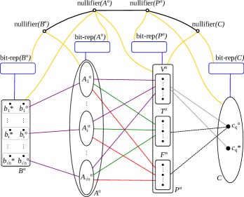
Figure 2: Overview of the reduction. Sets with elliptical (rectangular, resp.) boundaries are independent sets (cliques, resp.). For $X\in\{B^{\alpha},A^{\alpha},P^{\alpha},C\}$, the blue rectangle attached to it via the blue edge represents $\textsf{bit-rep}(X)$. We omit $\textsf{bits}(X)$ for legibility. The yellow line represents that $\textsf{nullifier}(X)$ is connected to every vertex in the set. Note the exception of $\textsf{nullifier}(P^{\alpha})$ which is not adjacent to any vertex in $A^{\alpha}$. Purple lines across two sets denote adjacencies with respect to indexing, i.e., $b^{\alpha,\circ}_{i}$ is adjacent only with all the vertices in $A^{\alpha}_{i}$, and all the vertices in $A^{\alpha}_{i}$ are adjacent with $v^{\alpha}_{i}$ in validation portal $V^{\alpha}$. Gray lines also indicate adjacencies with respect to indexing, but in a complementary way. If $C_{q}$ contains a variable in $B^{\alpha}_{i}$, then $c^{\circ}_{q}$ and $c^{\star}_{q}$ are adjacent with all vertices $v^{\alpha}_{j}\in V^{\alpha}$ such that $j\neq i$. Green and red lines across the $A^{\alpha}$ and $T^{\alpha}$ and $F^{\alpha}$ roughly transfer, for each $a_{i,\ell}^{\alpha}\in A^{\alpha}$, the underlying assignment structure. If the $j^{th}$ variable by $a_{i,\ell}^{\alpha}$ is assigned to True, then we add the green edge $(a_{i,\ell}^{\alpha},t_{j}^{\alpha})$, and otherwise the red edge $(a_{i,\ell}^{\alpha},f_{j}^{\alpha})$. Similarly, we add edges for each $c_{i}^{\circ}\in C$ depending on the assignment satisfying the variable from the part $X^{\delta}$ of a clause $c_{i}$, and in which block $B_{j}^{\delta}$ it lies, putting either an edge $(c_{i}^{\circ},t_{j}^{\delta})$ or $(c_{i}^{\circ},f_{j}^{\delta})$ accordingly ($\delta\in\{\alpha,\beta,\gamma\}$).

Now, we are ready to proceed through the final steps to complete the construction.

• For every clause $C_{q}$ in $\psi$, we introduce a pair of vertices $\langle c^{\circ}_{q},c^{\star}_{q}\rangle$. Let $C$ be the collection of vertices in such pairs. Then, we add a gadget as was described in Subsection 3.1.2 to make each pair $\langle c^{\circ}_{q},c^{\star}_{q}\rangle$ a critical one.

• We add edges across $C$ and the portals as follows for each $\delta\in\{\alpha,\beta,\gamma\}$. Consider a clause $C_{q}$ in $\psi$ and the corresponding critical pair $\langle c^{\circ}_{q},c^{\star}_{q}\rangle$ in $C$. As $\psi$ is an instance of $3$-Partitioned-$3$-SAT, there is at most one variable in $X^{\delta}$ that appears in $C_{q}$. Suppose that variable is $x^{\delta}_{i,j}$ for some $i,j\in[\sqrt{n}]$. The first subscript decides the edges across $\langle c^{\circ}_{q},c^{\star}_{q}\rangle$ and the validation portal, whereas the second subscript decides the edges across $\langle c^{\circ}_{q},c^{\star}_{q}\rangle$ and either the truth portal or false portal in the following sense. If $x^{\delta}_{i,j}$ appears in $C_{q}$, then we add all edges of the form $(v^{\delta}_{i^{\prime}},c^{\circ}_{q})$ and $(v^{\delta}_{i^{\prime}},c^{\star}_{q})$ for every $i^{\prime}\in[\sqrt{n}]$ such that $i^{\prime}\neq i$. If $x^{\delta}_{i,j}$ appears as a positive literal in $C_{q}$, then we add the edge $(t^{\delta}_{j},c^{\circ}_{q})$. If $x^{\delta}_{i,j}$ appears as a negative literal in $C_{q}$, then we add the edge $(f^{\delta}_{j},c^{\circ}_{q})$. Note that if $C_{q}$ does not contain a variable in $X^{\delta}$, then we make $c^{\circ}_{q}$ and $c^{\star}_{q}$ adjacent to every vertex in $V^{\delta}$, whereas they are not adjacent to any vertex in $T^{\delta}\cup F^{\delta}$. Finally, we add an edge between $\textsf{nullifier}(P^{\delta})$ and every vertex of $C$, and we add the edge $(\textsf{nullifier}(P^{\delta}),\textsf{nullifier}(C))$.

This concludes the construction of $G$. The reduction returns $(G,k)$ as an instance of Metric Dimension where

$$\begin{split}k&=3\cdot\left(\sqrt{n}+\left(\left\lceil\log(|B^{\alpha}|/2+2)\right\rceil+1\right)+\left(\left\lceil\log(|A^{\alpha}|+2)\right\rceil+1\right)+\left(\left\lceil\log(|P^{\alpha}|+2)\right\rceil+1\right)\right)+\\ &\lceil\log(|C|+2)\rceil+1.\end{split}$$

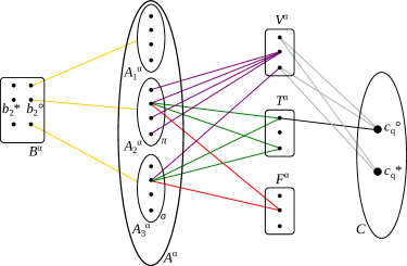
Figure 3: A toy example to illustrate the core ideas in the reduction. Note that bit-rep and nullifier are omitted for the sets.

We give an informal description of the proof of correctness here. See Figure 3. Suppose $\sqrt{n}=3$ and the vertices in the sets are indexed from top to bottom. For the sake of clarity, we do not show all the edges and only show $4$ out of $8$ vertices in each $A^{\alpha}_{i}$ for $i\in[3]$. We also omit bit-rep and nullifier for these sets. The vertex selection gadget and the budget $k$ ensure that exactly one vertex in $\{b^{\alpha,\circ}_{i},b^{\alpha,\star}_{i}\}\cup A^{\alpha}_{i}$ is selected for every $i\in[3]$. If a resolving set contains a vertex from $A^{\alpha}_{i}$, then it corresponds to selecting an assignment of variables in $X^{\alpha}_{i}$. For example, the vertex $a^{\alpha}_{2,2}$ corresponds to the assignment $\pi:X^{\alpha}_{2}\mapsto\{\texttt{True},\texttt{False}\}$. Suppose $X^{\alpha}_{2}=\{x^{\alpha}_{2,1},x^{\alpha}_{2,2},x^{\alpha}_{2,3}\}$, $\pi(x^{\alpha}_{2,1})=\pi(x^{\alpha}_{2,3})=\texttt{True}$, and $\pi(x^{\alpha}_{2,2})=\texttt{False}$. Hence, $a^{\alpha}_{2,2}$ is adjacent to the first and third vertex in the truth portal $T^{\alpha}$, whereas it is adjacent with the second vertex in the false portal $F^{\alpha}$. Suppose the clause $C_{q}$ contains the variable $x^{\alpha}_{2,1}$ as a positive literal. Note that $c^{\circ}_{q}$ and $c^{\star}_{q}$ are at distance $2$ and $3$, respectively, from $a^{\alpha}_{2,2}$. Hence, the vertex $a^{\alpha}_{2,2}$, corresponding to the assignment $\pi$ that satisfies clause $C_{q}$, resolves the critical pair $\langle c^{\circ}_{q},c^{\star}_{q}\rangle$. Now, suppose there is another assignment $\sigma:X^{\alpha}_{3}\mapsto\{\texttt{True},\texttt{False}\}$ such that $\sigma(x^{\alpha}_{3,1})=\sigma(x^{\alpha}_{3,3})=\texttt{True}$ and $\sigma(x^{\alpha}_{3,2})=\texttt{False}$. As $\psi$ is an instance of $3$-Partitioned-$3$-SAT and $C_{q}$ contains a variable in $X^{\alpha}_{2}$ ($\subseteq X^{\alpha}$), $C_{q}$ does not contain a variable in $X^{\alpha}_{3}$ ($\subseteq X^{\alpha}$). Hence, $\sigma$ does not satisfy $C_{q}$. Let $a^{\alpha}_{3,2}$ be the vertex in $X^{\alpha}_{3}$ corresponding to $\sigma$. The connections via the validation portal $V^{\alpha}$ ensure that both $c^{\circ}_{q}$ and $c^{\star}_{q}$ are at distance $2$ from $a^{\alpha}_{3,2}$, and hence, $a^{\alpha}_{3,2}$ cannot resolve the critical pair $\langle c^{\circ}_{q},c^{\star}_{q}\rangle$. Hence, finding a resolving set in $G$ corresponds to finding a satisfying assignment for $\psi$. These intuitions are formalized in the following subsection.

3.3 Correctness of the Reduction

Suppose, given an instance $\psi$ of $3$-Partitioned-$3$-SAT, that the reduction of this subsection returns $(G,k)$ as an instance of Metric Dimension. We first prove the following lemma which will be helpful in proving the correctness of the reduction.

Lemma 3.5.

For any resolving set $S$ of $G$ and for all $X\in\{B^{\delta},A^{\delta},P^{\delta},C\}$ and $\delta\in\{\alpha,\beta,\gamma\}$,

1. $S$ contains at least one vertex from each pair of false twins in $\textsf{bits}(X)$.

2. Vertices in $\textsf{bits}(X)\cap S$ resolve any non-critical pair of vertices $\langle u,v\rangle$ when $u\in X\cup X^{+}$ and $v\in V(G)$.

3. Vertices in $X^{+}\cap S$ cannot resolve any critical pair of vertices $\langle b_{i}^{\delta^{\prime},\circ},b_{i}^{\delta^{\prime},\star}\rangle$ nor $\langle c_{q}^{\circ},c_{q}^{\star}\rangle$ for all $i\in[\sqrt{n}]$, $\delta^{\prime}\in\{\alpha,\beta,\gamma\}$, and $q\in[m]$.

Proof 3.6.

1. By Section 2, the statement follows for all $X\in\{B^{\delta},A^{\delta},P^{\delta},C\}$ and $\delta\in\{\alpha,\beta,\gamma\}$.

2. For all $X\in\{B^{\delta},A^{\delta},P^{\delta},C\}$ and $\delta\in\{\alpha,\beta,\gamma\}$, note that $\textsf{nullifier}(X)$ is distinguished by $\textsf{bits}(X)$ since it is the only vertex in $G$ that is at distance $2$ from every vertex in $\textsf{bits}(X)$. We now do a case analysis for the remaining non-critical pairs of vertices $\langle u,v\rangle$ assuming that $\textsf{nullifier}(X)\notin\{u,v\}$ (also, suppose that both $u$ and $v$ are not in $S$, as otherwise, they are obviously distinguished):

   Case i: $u,v\in X\cup X^{+}$.

   Case i(a): $u,v\in X$ or $u,v\in\textsf{bit-rep}(X)\setminus\textsf{bits}(X)$.

   In the first case, let $j$ be the digit in the binary representation of the subscript of $u$ that is not equal to the $j^{\text{th}}$ digit in the binary representation of the subscript of $v$ (such a $j$ exists since $\langle u,v\rangle$ is not a critical pair). In the second case, without loss of generality, let $u=y_{i}$ and $v=y_{j}$. By the first item of the statement of the lemma (1.), without loss of generality, $y_{j}^{a}\in S\cap\textsf{bits}(X)$. Then, in both cases, $d(y_{j}^{a},u)\neq d(y_{j}^{a},v)$.

   Case i(b): $u\in X$ and $v\in\textsf{bit-rep}(X)$.

   Without loss of generality, $y_{\star}^{a}\in S\cap\textsf{bits}(X)$ (by 1.). Then, $d(y_{\star}^{a},u)=2$ and, for all $v\in\textsf{bits}(X)\setminus\{y_{\star}^{b}\}$, $d(y_{\star}^{a},v)=3$. Without loss of generality, let $y_{i}$ be adjacent to $u$ and let $y_{i}^{a}\in S\cap\textsf{bits}(X)$ (by 1.). Then, for $v=y_{\star}^{b}$, $3=d(y_{i}^{a},v)\neq d(y_{i}^{a},u)=2$. If $v\in\textsf{bit-rep}(X)\setminus\textsf{bits}(X)$, then, without loss of generality, $v=y_{j}$ and $y_{j}^{a}\in S\cap\textsf{bits}(X)$ (by 1.), and $1=d(y_{j}^{a},v)<d(y_{j}^{a},u)$.

   Case i(c): $u,v\in\textsf{bits}(X)$.

   Without loss of generality, $u=y_{i}^{b}$ and $y_{i}^{a}\in S$ (by 1.). Then, $2=d(y_{i}^{a},u)\neq d(y_{i}^{a},v)=3$.

   Case i(d): $u\in\textsf{bits}(X)$ and $v\in\textsf{bit-rep}(X)\setminus\textsf{bits}(X)$.

   Without loss of generality, $v=y_{i}$ and $y_{i}^{a}\in S$ (by 1.). Then, $1=d(y_{i}^{a},v)<d(y_{i}^{a},u)$.

   Case ii: $u\in X\cup X^{+}$ and $v\in V(G)\setminus(X\cup X^{+})$.

   For each $u\in X\cup X^{+}$, there exists $w\in\textsf{bits}(X)\cap S$ such that $d(u,w)\leq 2$, while, for each $v\in V(G)\setminus(X\cup X^{+})$ and $w\in\textsf{bits}(X)\cap S$, we have $d(v,w)\geq 3$.

3. For all $X\in\{B^{\delta},A^{\delta},P^{\delta}\}$, $\delta\in\{\alpha,\beta,\gamma\}$, $u\in X^{+}$, $v\in\{c_{q}^{\circ},c_{q}^{\star}\}$, and $q\in[m]$, we have that $d(u,v)=d(u,\textsf{nullifier}(P^{\delta}))+1$. Further, for $X=C$ and all $u\in X^{+}$ and $q\in[m]$, either $d(u,c_{q}^{\circ})=d(u,c_{q}^{\star})=1$, $d(u,c_{q}^{\circ})=d(u,c_{q}^{\star})=2$, or $d(u,c_{q}^{\circ})=d(u,c_{q}^{\star})=3$ by the construction in Subsection 3.1.2 and since $\textsf{bit-rep}(X)\setminus\textsf{bits}(X)$ is a clique. Hence, for all $X\in\{B^{\delta},A^{\delta},P^{\delta},C\}$ and $\delta\in\{\alpha,\beta,\gamma\}$, vertices in $X^{+}\cap S$ cannot resolve a pair of vertices $\langle c_{q}^{\circ},c_{q}^{\star}\rangle$ for any $q\in[m]$.

   For all $\delta\in\{\alpha,\beta,\gamma\}$, if $v\in B^{\delta}$, then, for all $X\in\{B^{\delta^{\prime}},A^{\delta^{\prime}},P^{\delta^{\prime}},C\}$, $\delta^{\prime}\in\{\alpha,\beta,\gamma\}$ such that $\delta\neq\delta^{\prime}$, and $u\in X^{+}$, we have that $d(u,v)=d(u,\textsf{nullifier}(A^{\delta}))+1$. Similarly, for all $\delta\in\{\alpha,\beta,\gamma\}$, if $v\in B^{\delta}$, then, for all $X\in\{A^{\delta},P^{\delta}\}$ and $u\in X^{+}$, we have that $d(u,v)=d(u,\textsf{nullifier}(A^{\delta}))+1$. Lastly, for each $\langle b_{i}^{\delta,\circ},b_{i}^{\delta,\star}\rangle$, $\delta\in\{\alpha,\beta,\gamma\}$, and $i\in[\sqrt{n}]$, if $X=B^{\delta}$, then, for all $u\in X^{+}$, either $d(u,b_{i}^{\delta,\circ})=d(u,b_{i}^{\delta,\star})=1$, $d(u,b_{i}^{\delta,\circ})=d(u,b_{i}^{\delta,\star})=2$, or $d(u,b_{i}^{\delta,\circ})=d(u,b_{i}^{\delta,\star})=3$ by the construction in Subsection 3.1.2 and since $\textsf{bit-rep}(X)\setminus\textsf{bits}(X)$ is a clique.

Lemma 3.7.

If $\psi$ is a satisfiable $3$-Partitioned-$3$-SAT formula, then $G$ admits a resolving set of size $k$.

Proof 3.8.

Suppose $\pi:X^{\alpha}\cup X^{\beta}\cup X^{\gamma}\mapsto\{\texttt{True},\texttt{False}\}$ is a satisfying assignment for $\psi$. We construct a resolving set $S$ of size $k$ for $G$ using this assignment.

Initially, set $S=\emptyset$. For every $\delta\in\{\alpha,\beta,\gamma\}$ and $i\in[\sqrt{n}]$, consider the assignment $\pi$ restricted to the variables in $X^{\delta}_{i}$. By the construction, there is a vertex in $A^{\delta}_{i}$ that corresponds to this assignment. Include that vertex in $S$. For each $X\in\{B^{\delta},A^{\delta},P^{\delta},C\}$, where $\delta\in\{\alpha,\beta,\gamma\}$, we add one vertex from each pair of the false twins in $\textsf{bits}(X)$ to $S$. Note that $|S|=k$ and that every vertex in $S$ is distinguished by itself.

In the remaining part of the proof, we show that $S$ is a resolving set of $G$. First, we prove that all critical pairs are resolved by $S$ in the following claim.

Claim 1.

All critical pairs are resolved by $S$.

For each $i\in[\sqrt{n}]$ and $\delta\in\{\alpha,\beta,\gamma\}$, the critical pair $\langle b^{\delta,\circ}_{i},b^{\delta,\star}_{i}\rangle$ is resolved by the vertex $S\cap A_{i}^{\delta}$ by the construction. For each $q\in[m]$, the clause $C_{q}$ is satisfied by the assignment $\pi$. Thus, there is a variable $x$ in $C_{q}$ that satisfies $C_{q}$ according to $\pi$. Suppose that $x\in X_{i}^{\delta}$. Let $a_{i,\ell}^{\delta}$ be the vertex in $A_{i}^{\delta}$ corresponding to $\pi$. Then, by the construction, $d(a_{i,\ell}^{\delta},c_{q}^{\circ})=2<3=d(a_{i,\ell}^{\delta},c_{q}^{\star})$. Thus, every critical pair $\langle c_{q}^{\circ},c_{q}^{\star}\rangle$ is resolved by $S$.

Then, every vertex pair in $V(G)$ is resolved by $S$ by Claim 1 in conjunction with the second item of the statement of Lemma 3.5.

Lemma 3.9.

If $G$ admits a resolving set of size $k$, then $\psi$ is a satisfiable $3$-Partitioned-$3$-SAT formula.

Proof 3.10.

Assume that $G$ admits a resolving set $S$ of size $k$. First, we prove some properties regarding $S$. By the first item of the statement of Lemma 3.5, for each $\delta\in\{\alpha,\beta,\gamma\}$, we have that

$$|S\cap\textsf{bits}(A^{\delta})|\geq\lceil\log(|A^{\delta}|+2)\rceil+1,\qquad\, |S\cap\textsf{bits}(P^{\delta})|\geq\lceil\log(|P^{\delta}|+2)\rceil+1,$$

$$|S\cap\textsf{bits}(B^{\delta})|\geq\lceil\log(|B^{\delta}|/2+2)\rceil+1,\quad |S\cap\textsf{bits}(C)|\geq\lceil\log(|C|+2)\rceil+1.$$

Hence, any resolving set $S$ of $G$ already has size at least

$$3\cdot\left(\left(\left\lceil\log(|B^{\alpha}|/2+2)\right\rceil+1\right)+\left(\left\lceil\log(|A^{\alpha}|+2)\right\rceil+1\right)+\left(\left\lceil\log(|P^{\alpha}|+2)\right\rceil+1\right)\right)+\lceil\log(|C|+2)\rceil+1.$$

Now, for each $\delta\in\{\alpha,\beta,\gamma\}$ and $i\in[\sqrt{n}]$, consider the critical pair $\langle b_{i}^{\delta,\circ},b_{i}^{\delta,\star}\rangle$. By the construction mentioned in Subsection 3.1.2, only $v\in A_{i}^{\delta}\cup\{b_{i}^{\delta,\circ},b_{i}^{\delta,\star}\}$ resolves a pair $\langle b_{i}^{\delta,\circ},b_{i}^{\delta,\star}\rangle$. Indeed, for all $X\in\{B^{\delta^{\prime}},A^{\delta^{\prime}},P^{\delta^{\prime}},C\}$ and $\delta^{\prime}\in\{\alpha,\beta,\gamma\}$, no vertex in $X^{+}$ can resolve such a pair by the third item of the statement of Lemma 3.5. Also, for all $X\in\{A^{\delta^{\prime\prime}},P^{\delta^{\prime}},C\}$, $\delta^{\prime}\in\{\alpha,\beta,\gamma\}$, $\delta^{\prime\prime}\in\{\alpha,\beta,\gamma\}$ such that $\delta\neq\delta^{\prime\prime}$, and $u\in X$, we have that $d(u,b_{i}^{\delta,\circ})=d(u,b_{i}^{\delta,\star})=d(u,\textsf{nullifier}(A^{\delta}))+1$. Furthermore, for any $a\in A_{j}^{\delta}$ with $j\in[\sqrt{n}]$ such that $i\neq j$, we have that $d(a,b_{i}^{\delta,\circ})=d(a,b_{i}^{\delta,\star})=2$ by construction and since $B^{\delta}$ is a clique. Hence, since any resolving set $S$ of $G$ of size at most $k$ can only admit at most another $3\sqrt{n}$ vertices, we get that equality must in fact hold in every one of the aforementioned inequalities, and any resolving set $S$ of $G$ of size at most $k$ contains one vertex from $A_{i}^{\delta}\cup\{b_{i}^{\delta,\circ},b_{i}^{\delta,\star}\}$ for all $i\in[\sqrt{n}]$ and $\delta\in\{\alpha,\beta,\gamma\}$. Hence, any resolving set $S$ of $G$ of size at most $k$ is actually of size exactly $k$.

Next, for each $\delta\in\{\alpha,\beta,\gamma\}$, we construct an assignment $\pi:X^{\alpha}\cup X^{\beta}\cup X^{\gamma}\mapsto\{\texttt{True},\texttt{False}\}$ in the following way. If $a_{i,\ell}^{\delta}\in S$ and $\pi^{\prime}:X_{i}^{\delta}\rightarrow\{\texttt{True},\texttt{False}\}$ corresponds to the underlying assignment of $a_{i,\ell}^{\delta}$ for the variables in $X_{i}^{\delta}$, then let $\pi:X_{i}^{\delta}\rightarrow\{\texttt{True},\texttt{False}\}:=\pi^{\prime}$ for each $i\in[\sqrt{n}]$ and $\delta\in\{\alpha,\beta,\gamma\}$. If $S\cap A_{i}^{\delta}=\emptyset$, then one of $b_{i}^{\delta,\circ},b_{i}^{\delta,\star}$ is in $S$, and we can use an arbitrary assignment of the variables in the bucket $X_{i}^{\delta}$.

We contend that the constructed assignment $\pi$ satisfies every clause in $C$. Since $S$ is a resolving set, it follows that, for every clause $c_{q}\in C$, there exists $v\in S$ such that $d(v,c_{q}^{\circ})\neq d(v,c_{q}^{\star})$. Notice that, for any $v$ in $\textsf{bits}(A^{\delta}),\textsf{bits}(B^{\delta}),\textsf{bits}(P^{\delta})$ for any $\delta\in\{\alpha,\beta,\gamma\}$ or in $\textsf{bits}(C)$, we have $d(v,c_{q}^{\circ})=d(v,c_{q}^{\star})$ by the third item of the statement of Lemma 3.5. Further, for any $v\in B^{\delta}$ and any $\delta\in\{\alpha,\beta,\gamma\}$, we have that $d(v,c_{q}^{\circ})=d(v,c_{q}^{\star})=d(v,\textsf{nullifier}(P^{\delta}))+1$. Thus, $v\in S\cap\bigcup\limits_{\delta\in\{\alpha,\beta,\gamma\}}A^{\delta}$. Without loss of generality, suppose that $c_{q}^{\circ}$ and $c_{q}^{\star}$ are resolved by $a_{i,\ell}^{\alpha}$. So, $d(a_{i,\ell}^{\alpha},c_{q}^{\circ})\neq d(a_{i,\ell}^{\alpha},c_{q}^{\star})$. By the construction, the only case where $d(a_{i,\ell}^{\alpha},c_{q}^{\circ})\neq d(a_{i,\ell}^{\alpha},c_{q}^{\star})$ is when $C_{q}$ contains a variable $x\in X_{i}^{\alpha}$ and $\pi(x)$ satisfies $C_{q}$. Thus, we get that the clause $C_{q}$ is satisfied by the assignment $\pi$.

Since $S$ resolves all pairs $\langle c_{q}^{\circ},c_{q}^{\star}\rangle$ in $V(G)$, then the assignment $\pi$ constructed above indeed satisfies every clause $c_{q}$, completing the proof.

Proof 3.11 Proof of Theorem 3.1..

The proof of Proposition 2.2, relies on the fact that there is a polynomial-time reduction from 3-SAT to $3$-Partitioned-$3$-SAT that increases the number of variables and clauses by a constant factor. In Subsection 3.2, we presented a reduction that takes an instance $\psi$ of $3$-Partitioned-$3$-SAT and returns an equivalent instance $(G,k)$ of Metric Dimension (by Lemmas 3.7 and 3.9) in $2^{\mathcal{O}(\sqrt{n})}$ time. Note that $V(G)=2^{\mathcal{O}(\sqrt{n})}$. Further, note that taking all the vertices in $B^{\delta}$, $P^{\delta}$, and $\textsf{bit-rep}(X)$ for all $X\in\{B^{\delta},A^{\delta},P^{\delta},C\}$ and $\delta\in\{\alpha,\beta,\gamma\}$, results in a vertex cover of $G$. Hence,

$$\begin{split}\mathtt{vc}(G)&\leq 3\cdot\left(\left(\left\lceil\log(|B^{\alpha}|/2+2)\right\rceil+1\right)+\left(\left\lceil\log(|A^{\alpha}|+2)\right\rceil+1\right)+\left(\left\lceil\log(|P^{\alpha}|+2)\right\rceil+1\right)\right)+\\ &3\cdot(|B^{\alpha}|+|P^{\alpha}|)+(\lceil\log(|C|+2)\rceil+1)=\mathcal{O}(\sqrt{n}).\end{split}$$

Lastly, the metric dimension of $G$ is at most

$$\begin{split}k&=3\cdot\left(\sqrt{n}+\left(\left\lceil\log(|B^{\alpha}|/2+2)\right\rceil+1\right)+\left(\left\lceil\log(|A^{\alpha}|+2)\right\rceil+1\right)+\left(\left\lceil\log(|P^{\alpha}|+2)\right\rceil+1\right)\right)+\\ &(\lceil\log(|C|+2)\rceil+1)=\mathcal{O}(\sqrt{n}).\end{split}$$

Thus, $\mathtt{vc}(G)+k=\mathcal{O}(\sqrt{n})$.

4 Geodetic Set: Lower Bounds Regarding Vertex Cover

In this section, we follow the same template as in Section 3 and first prove the following theorem.

Theorem 4.1.

There is an algorithm that, given an instance $\psi$ of 3-Partitioned-3-SAT on $N$ variables, runs in time $2^{\mathcal{O}(\sqrt{N})}$, and constructs an equivalent instance $(G,k)$ of Geodetic Set such that $\mathtt{vc}(G)+k=\mathcal{O}(\sqrt{N})$ (and $|V(G)|=2^{\mathcal{O}(\sqrt{N})}$).

The proofs of the following two corollaries are analogous to the ones in the previous section.

Corollary 4.2.

Unless the ETH fails, Geodetic Set does not admit an algorithm running in time $2^{o(\mathtt{vc}^{2})}\cdot n^{\mathcal{O}(1)}$.

Corollary 4.3.

Unless the ETH fails, Geodetic Set does not admit a kernelization algorithm that reduces the solution size $k$ and outputs a kernel with $2^{o(k+\mathtt{vc})}$ vertices.

4.1 Reduction

Consider an instance $\psi$ of 3-Partitioned-3-SAT with $X^{\alpha},X^{\beta},X^{\gamma}$ the partition of the variable set, where $|X^{\alpha}|=|X^{\beta}|=|X^{\gamma}|=n$. By adding dummy variables in each of these sets, we can assume that $\sqrt{n}$ is an integer. Further, let $\mathcal{C}=\{C_{1},\dots,C_{m}\}$ be the set of all the clauses of $\psi$. From $\psi$, we construct the graph $G$ as follows. We describe the first part of the construction for $X^{\alpha}$, with the constructions for $X^{\beta}$ and $X^{\gamma}$ being analogous. We rename the variables in $X^{\alpha}$ to $x^{\alpha}_{i,j}$ for $i,j\in[\sqrt{n}]$.

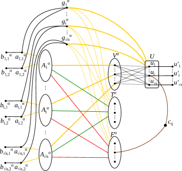
Figure 4: Overview of the reduction. Sets with elliptical boundaries are independent sets, and sets with rectangular boundaries are cliques. For each $\delta\in\{\alpha,\beta,\gamma\}$, the sets $V^{\delta}$ and $U$ almost form a complete bipartite graph modulo the matching (marked by dotted edges), which is excluded. Yellow lines from a vertex to a set denote that this vertex is connected to all the vertices in that set. The green and red lines across the $A_{i}^{\alpha}$ and $T^{\alpha}\cup F^{\alpha}$ transfer, in some sense, for each $w\in A_{i}^{\alpha}$, the underlying assignment structure. If an underlying assignment $w$ sets the $j^{th}$ variable to True, then we add the green edge $(w,t_{j}^{\alpha})$, and otherwise, we add the red edge $(w,f_{j}^{\alpha})$. For all $q\in[m]$ and $\delta\in\{\alpha,\beta,\gamma\}$, let $x_{i,j}^{\delta}$ be the variable in $X^{\delta}$ that is contained in the clause $C_{q}$ in $\psi$. So, for all $q\in[m]$, if assigning True (False, respectively) to $x_{i,j}^{\delta}$ satisfies $C_{q}$, then we add the edge $(c_{q},t_{j}^{\delta})$ ($(c_{q},f_{j}^{\delta})$, respectively).

• We partition the variables of $X^{\alpha}$ into buckets $X^{\alpha}_{1},X^{\alpha}_{2},\dots,X^{\alpha}_{\sqrt{n}}$ such that each bucket contains $\sqrt{n}$ many variables. Let $X^{\alpha}_{i}=\{x^{\alpha}_{i,j}\ |\ j\in[\sqrt{n}]\}$ for all $i\in[\sqrt{n}]$.

• For every bucket $X^{\alpha}_{i}$, we add an independent set $A^{\alpha}_{i}$ of $2^{\sqrt{n}}$ new vertices, and we add two isolated edges $(a^{\alpha}_{i,1},b^{\alpha}_{i,1})$ and $(a^{\alpha}_{i,2},b^{\alpha}_{i,2})$. Let $B^{\alpha}=\{a^{\alpha}_{i,j},b^{\alpha}_{i,j}\mid i\in[\sqrt{n}],j\in\{1,2\}\}$. For all $i\in[\sqrt{n}]$ and $u\in A_{i}^{\alpha}$, we make both $a^{\alpha}_{i,1}$ and $a^{\alpha}_{i,2}$ adjacent to $u$ (see Figure 4).

  Each vertex in $A^{\alpha}_{i}$ corresponds to a certain possible assignment of variables in $X^{\alpha}_{i}$.

• Then, we add three independent sets $T^{\alpha}$, $F^{\alpha}$, and $V^{\alpha}$ on $\sqrt{n}$ vertices each: $T^{\alpha}=\{t^{\alpha}_{i}\mid i\in[\sqrt{n}]\}$, $F^{\alpha}=\{f^{\alpha}_{i}\mid i\in[\sqrt{n}]\}$, and $V^{\alpha}=\{v^{\alpha}_{i}\mid i\in[\sqrt{n}]\}$.

• For each $i\in[\sqrt{n}]$, we connect $v^{\alpha}_{i}$ with all the vertices in $A^{\alpha}_{i}$.

• For each $i\in[\sqrt{n}]$, we add a special vertex $g^{\alpha}_{i}$ (also referred to as a $g$-vertex later on) that is adjacent to each vertex in $T^{\alpha}\cup F^{\alpha}$. Further, $g^{\alpha}_{i}$ is also adjacent to both $a^{\alpha}_{i,1}$ and $a^{\alpha}_{i,2}$ (see Figure 4).

This finishes the first part of the construction. The second step is to connect the three previously constructed parts for $X^{\alpha}$, $X^{\beta}$, and $X^{\gamma}$.

• We introduce a vertex set $U=\{u_{i}\mid i\in[\sqrt{n}]\}$ that forms a clique. Then, for each $u_{i}$, we add an edge to a new vertex $u^{\prime}_{i}$. Thus, we have a matching $\{(u_{i},u^{\prime}_{i})\mid i\in[\sqrt{n}]\}$. Let $U^{\prime}=\{u^{\prime}_{i}\mid i\in[\sqrt{n}]\}$.

• For each $\delta\in\{\alpha,\beta,\gamma\}$, we make it so that the vertices of $U\cup V^{\delta}$ form almost a complete bipartite graph, i.e., $E(G)$ contains edges between all pairs $\langle v,w\rangle$ where $v\in U$ and $w\in V^{\delta}$, except for the matching $\{(v^{\delta}_{i},u_{i})\mid i\in[\sqrt{n}]\}$.

• For each $\delta\in\{\alpha,\beta,\gamma\}$ and $i\in[\sqrt{n}]$, we make $g_{i}^{\delta}$ adjacent to each vertex in $U$.

• For each $C_{q}\in\mathcal{C}$, we add a new vertex $c_{q}$. Let $C=\{c_{q}\mid q\in[m]\}$. Since we are considering an instance of 3-Partitioned-3-SAT, for each $\delta\in\{\alpha,\beta,\gamma\}$, there is exactly one variable in $C_{q}$ that lies in $X^{\delta}_{i}$, and, without loss of generality, let it be $x_{i,j}^{\delta}$. Then, we make $c_{q}$ adjacent to $u_{i}$. Finally, if $x_{i,j}^{\delta}=\texttt{True}$ ($x_{i,j}^{\delta}=\texttt{False}$, respectively) satisfies $C_{q}$, then $(c_{q},t^{\delta}_{j})\in E(G)$ ($(c_{q},f^{\delta}_{j})\in E(G)$, respectively).

This concludes the construction of $G$. The reduction returns $(G,k)$ as an instance of Geodetic Set where $k=10\sqrt{n}$.

4.2 Correctness of the Reduction

Suppose, given an instance $\psi$ of $3$-Partitioned-$3$-SAT, that the reduction above returns $(G,k)$ as an instance of Geodetic Set. We first prove the following lemmas which will be helpful in proving the correctness of the reduction, and note that we use distances between vertices to prove that certain vertices are not contained in shortest paths.

Lemma 4.4.

For all $\delta,\delta^{\prime}\in\{\alpha,\beta,\gamma\}$, the shortest paths between any two vertices in $B^{\delta}\cup U\cup U^{\prime}$ do not cover any vertices in $C$ nor $V^{\delta^{\prime\prime}}$.

Proof 4.5.

Since, for all $i\in[\sqrt{n}]$, $j\in\{1,2\}$, and $\delta\in\{\alpha,\beta,\gamma\}$, the shortest path from $b_{i,j}^{\delta}$ ($u^{\prime}_{i}$, respectively) to any other vertex in $G$ first passes through $a_{i,j}^{\delta}$ ($u_{i}$, respectively), it suffices to prove the statement of the lemma for the shortest paths between any two vertices in $U\cup(B^{\delta}\setminus\{b_{i,j}^{\delta}\mid i\in[\sqrt{n}],j\in\{1,2\}\})$.

For all $i\in[\sqrt{n}]$, $j\in\{1,2\}$, and $\delta,\delta^{\prime}\in\{\alpha,\beta,\gamma\}$, we have $d(a_{i,1}^{\delta},a_{i,2}^{\delta})=2$ and $d(a_{i,j}^{\delta},w)\geq 2$ for all $w\in V^{\delta^{\prime}}\cup C$. For all $i,i^{\prime}\in[\sqrt{n}]$, $j,j^{\prime}\in\{1,2\}$, and $\delta,\delta^{\prime},\delta^{\prime\prime}\in\{\alpha,\beta,\gamma\}$ such that $i\neq i^{\prime}$ and/or $\delta\neq\delta^{\prime}$ (i.e., we are not in the previous case), we have $d(a_{i,j}^{\delta},a_{i^{\prime},j^{\prime}}^{\delta^{\prime}})=4$, $d(a_{i,j}^{\delta},w)=d(a_{i^{\prime},j^{\prime}}^{\delta^{\prime}},w)=3$ for all $w\in C$, and, for any $w^{\prime}\in V^{\delta^{\prime\prime}}$, we have $d(a_{i,j}^{\delta},w^{\prime})\geq 2$, $d(a_{i^{\prime},j^{\prime}}^{\delta^{\prime}},w^{\prime})\geq 2$, and $3\in\{d(a_{i,j}^{\delta},w^{\prime}),d(a_{i^{\prime},j^{\prime}}^{\delta^{\prime}},w^{\prime})\}$. Further, for any $i,i^{\prime}\in[\sqrt{n}]$ with $i\neq i^{\prime}$, $d(u_{i},u_{i^{\prime}})=1$. Lastly, for all $i,i^{\prime}\in[\sqrt{n}]$, $j\in\{1,2\}$, and $\delta,\delta^{\prime}\in\{\alpha,\beta,\gamma\}$, we have $d(a_{i,j}^{\delta},u_{i^{\prime}})=2$, while $d(a_{i,j}^{\delta},w)\geq 2$ for all $w\in V^{\delta^{\prime}}\cup C$. Hence, the vertices in $C$ and $V^{\delta^{\prime}}$ are not covered by any shortest path between any of these pairs.

Lemma 4.6.

For all $i\in[\sqrt{n}]$ and $\delta\in\{\alpha,\beta,\gamma\}$, $v_{i}^{\delta}$ can only be covered by a shortest path from a vertex in $A_{i}^{\delta}\cup\{v_{i}^{\delta}\}$ to another vertex in $G$.

Proof 4.7.

As stated in the proof of Lemma 4.4, we do not need to consider any shortest path with an endpoint that is a degree-$1$ vertex. First, we show that $v_{i}^{\delta}$ cannot be covered by a shortest path with one endpoint in $U$ and the other not in $A_{i}^{\delta}\cup\{v_{i}^{\delta}\}$. To cover this case, by Lemma 4.4, we just need to consider all shortest paths between a vertex $w\in U$ and any other vertex $z\in V(G)\setminus(U\cup U^{\prime}\cup B^{\alpha}\cup B^{\beta}\cup B^{\gamma}\cup A_{i}^{\delta}\cup\{v_{i}^{\delta}\})$. Note that $d(z,v_{i}^{\delta})\geq 2)$, and so, if $d(w,z)\leq 2$, then $v_{i}^{\delta}$ is not covered by the pair $\langle w,z\rangle$. Further, $d(w,w^{\prime})\leq 3$ for all $w^{\prime}\in V(G)$, and, for all $z^{\prime}\in V(G)$ such that $d(w,z^{\prime})=3$, we have that $d(z^{\prime},v_{i}^{\delta})\geq 3$. Hence, $v_{i}^{\delta}$ cannot be covered by a shortest path with one endpoint in $U$ and the other not in $A_{i}^{\delta}\cup\{v_{i}^{\delta}\}$.

For all $i\in[\sqrt{n}]$ and $\delta\in\{\alpha,\beta,\gamma\}$, we have that $N(v_{i}^{\delta})=A^{\alpha}_{i}\cup(U\setminus\{u_{i}\})$, and $d(w,z)\leq 2$ for any $w,z\in N(v_{i}^{\delta})$. Hence, for a shortest path between two vertices in $V(G)\setminus(A_{i}^{\delta}\cup\{v_{i}^{\delta}\})$ to contain $v_{i}^{\delta}$, that path must also contain two vertices from $N(v_{i}^{\delta})$. Furthermore, since $v_{i}^{\delta}$ cannot be covered by a shortest path with one endpoint in $U$ and the other not in $A_{i}^{\delta}\cup\{v_{i}^{\delta}\}$, any shortest path whose endpoints are in $V(G)\setminus(A_{i}^{\delta}\cup\{v_{i}^{\delta})\}$ that could cover $v_{i}^{\delta}$ cannot have any of its endpoints in $N(v_{i}^{\delta})$, and thus, must have length at least $4$. In particular, this proves the following property that we put as a claim to make reference to later.

Claim 2.

For any shortest path whose endpoints cannot be in $N[v_{i}^{\delta}]$, if its first and second endpoints are at distance at least $\ell_{1}$ and $\ell_{2}$, respectively, from any vertex in $N(v_{i}^{\delta})$, then this shortest path cannot cover $v_{i}^{\delta}$ if it has length less than $\ell_{1}+\ell_{2}+2$.

We finish with a case analysis of the possible pairs $\langle u,v\rangle$ to prove that no such shortest path covering $v_{i}^{\delta}$ exists using 2. We note that, by the arguments above, we do not need to consider the case where $u$ and/or $v$ is a degree-$1$ vertex, nor the case where both $u$ and $v$ are in $U\cup B^{\alpha}\cup B^{\beta}\cup B^{\gamma}$, nor the case where one of $u$ and $v$ is in $U$. We now proceed with the case analysis assuming that $u,v\notin N[v_{i}^{\delta}]$.

• Case 1: $\bm{u\in A_{i^{\prime}}^{\delta^{\prime}}}$ for any $\mathbf{i^{\prime}\in[\sqrt{n}]}$ and $\bm{\delta^{\prime}\in\{\alpha,\beta,\gamma\}}$ such that $\bm{A_{i^{\prime}}^{\delta^{\prime}}\neq A_{i}^{\delta}}$. First, $u$ is at distance at least $2$ from any vertex in $N(v_{i}^{\delta})$, and hence, if $d(u,v)\leq 4$, then we are done by 2. Note that $d(u,v)\leq 4$ as long as $v\notin A_{i^{\prime}}^{\delta^{\prime\prime}}$ for any $\delta^{\prime\prime}\in\{\alpha,\beta,\gamma\}$ such that $\delta^{\prime\prime}\neq\delta^{\prime}$, since $u$ is at distance $2$ from every vertex in $U\setminus\{u_{i^{\prime}}\}$. However, in the case where $v\in A_{i^{\prime}}^{\delta^{\prime\prime}}$, we have that $v$ is also at distance at least $2$ from any vertex in $N(v_{i}^{\delta})$, and so, since $d(u,v)\leq 5$, we are done by 2.

• Case 2: $\mathbf{u\in C}$ or $\mathbf{u}$ is a $\mathbf{g}$-vertex. By 2 and the previous case, it suffices to note that $d(u,v)\leq 3$ as long as $v\notin A_{i^{\prime}}^{\delta^{\prime}}$ for any $i^{\prime}\in[\sqrt{n}]$ and $\delta^{\prime}\in\{\alpha,\beta,\gamma\}$.

• Case 3: $\bm{u\in T^{\delta^{\prime}}\cup F^{\delta^{\prime}}}$ for any $\bm{\delta^{\prime}\in\{\alpha,\beta,\gamma\}}$ such that $\mathbf{\bm{\delta}^{\prime}\neq\bm{\delta}}$. Since $u$ is at distance $2$ from any vertex in $U$, we have that $d(u,v)\leq 4$, and we are done by 2.

• Case 4: $\bm{u\in T^{\delta}\cup F^{\delta}}$. First, if $v\notin A_{i^{\prime}}^{\delta^{\prime}}$ for any $i^{\prime}\in[\sqrt{n}]$ and $\delta^{\prime}\in\{\alpha,\beta,\gamma\}$, and $v$ is a vertex with a superscript $\delta$, then $d(u,v)\leq 3$. Otherwise, the path from $u$ to $v$ contains a vertex in $U\cup C$, and thus, does not cover $v_{i}^{\delta}$ since $d(u,v_{i}^{\delta})\geq 2$, $u$ is at distance $2$ (at most $3$, respectively) from any vertex in $U$ ($C$, respectively), and $v_{i}^{\delta}$ is at distance at least $2$ from any vertex in $C$. Thus, we are done by the previous cases and 2.

• Case 5: $\bm{u\in V^{\delta^{\prime}}}$ for any $\bm{\delta^{\prime}\in\{\alpha,\beta,\gamma\}}$. For any $\delta^{\prime\prime}\in\{\alpha,\beta,\gamma\}$, if $v\in B^{\delta^{\prime\prime}}\cup V^{\delta^{\prime\prime}}$, then $d(u,v)\leq 3$, and we are done by the previous cases and 2.

Lemma 4.8.

If $G$ admits a geodetic set of size $k$, then $\psi$ is a satisfiable $3$-Partitioned-$3$-SAT formula.

Proof 4.9.

Assume that $G$ admits a geodetic set $S$ of size $k$. Then, let us consider the set $S^{\prime}=\{u_{i}^{\prime}\mid i\in[\sqrt{n}]\}\cup\{b^{\delta}_{i,1},b^{\delta}_{i,2}\mid\delta\in\{\alpha,\beta,\gamma\},i\in[\sqrt{n}]\}$ of all the degree-1 vertices in $G$. By 2.1, $S^{\prime}\subseteq S$. By Lemma 4.6, for each $i\in[\sqrt{n}]$ and $\delta\in\{\alpha,\beta,\gamma\}$, there is at least one vertex from $A_{i}^{\delta}\cup\{v_{i}^{\delta}\}$ in $S$. Since $|S^{\prime}|=7\sqrt{n}$ and $k=10\sqrt{n}$, for each $i\in[\sqrt{n}]$ and $\delta\in\{\alpha,\beta,\gamma\}$, $S$ contains exactly $1$ vertex from $A_{i}^{\delta}\cup\{v_{i}^{\delta}\}$.

By Lemma 4.4, the shortest paths between vertices in $S^{\prime}$ do not cover vertices in $C$, and thus, the $3\sqrt{n}$ vertices in $S\setminus S^{\prime}$ must cover them.

For this goal, the vertices in $S$ that are in $V^{\delta}$ for any $\delta\in\{\alpha,\beta,\gamma\}$ are irrelevant. Indeed, any such vertex is at distance at most $3$ from any other vertex in $S\setminus S^{\prime}$, while every vertex in $S\setminus S^{\prime}$ is at distance at least $2$ from any vertex in $C$. So, let us consider one vertex from $A^{\delta}$ for some $\delta\in\{\alpha,\beta,\gamma\}$ that lies in $S$, say, without loss of generality, $w\in A_{i}^{\alpha}$. Note that $d(w,u^{\prime}_{i})=4$ and recall that $u^{\prime}_{i}\in S$. For any $q\in[m]$, there is a path of length $4$ between $w$ and $u^{\prime}_{i}$ that covers $c_{q}$ if there is $v\in T^{\alpha}\cup F^{\alpha}$ such that both $(w,v)$ and $(v,c_{q})$ are in $E(G)$. But, by the construction, such an edge $(w,v)\in E(G)$ corresponds to an assignment of a variable that occurs in $c_{q}$, i.e., $(v,c_{q})\in E(G)$ if the corresponding assignment to $v$ (True or False) satisfies the clause $C_{q}$ of the instance $\psi$. Since $S$ is a geodetic set, for each $q\in[m]$, there is a vertex $w\in\bigcup_{\delta\in\{\alpha,\beta,\gamma\}}A^{\delta}\cap S$ that covers $c_{q}$ by a shortest path to some $u\in U^{\prime}$. Thus, let $\pi:X^{\alpha}\cup X^{\beta}\cup X^{\gamma}\rightarrow\{\texttt{True},\texttt{False}\}$ be the retrieved assignment from the partial assignments that correspond to such vertices $w$ that are in both $S$ and $\bigcup_{\delta\in\{\alpha,\beta,\gamma\}}A^{\delta}$, and that is completed by selecting an arbitrary assignment for the variables in the buckets $X_{i}^{\delta}$ where $A_{i}^{\alpha}\cap S=\emptyset$.

Finally, as we observed above, for each $q\in[m]$, $c_{q}$ is covered, and thus, the constructed assignment $\pi$ satisfies all the clauses in $\mathcal{C}$.

Lemma 4.10.

If $\psi$ is a satisfiable $3$-Partitioned-$3$-SAT formula, then $G$ admits a geodetic set of size $k$.

Proof 4.11.

Suppose $\pi:X^{\alpha}\cup X^{\beta}\cup X^{\gamma}\rightarrow\{\texttt{True},\texttt{False}\}$ is a satisfying assignment for $\psi$. We construct a geodetic set $S$ of size $k$ for $G$ using this assignment. Initially, let

$$S=\{u_{i}^{\prime}\mid i\in[\sqrt{n}]\}\cup\{b^{\delta}_{i,1},b^{\delta}_{i,2}\mid\delta\in\{\alpha,\beta,\gamma\},i\in[\sqrt{n}]\}.$$

At this point, $|S|=7\sqrt{n}$. Now, for each $i\in[\sqrt{n}]$ and $\delta\in\{\alpha,\beta,\gamma\}$, we add one vertex from $A^{\delta}_{i}$ to $S$ in the following way. For the bucket of variables $X^{\delta}_{i}$, consider how the variables of $X^{\delta}_{i}$ are assigned by $\pi$, and denote this assignment restricted to $X^{\delta}_{i}$ by $\pi^{\delta}_{i}$. Since $A^{\delta}_{i}$ contains a vertex for each of the possible $2^{\sqrt{n}}$ assignments and each of those corresponds to a certain assignment of $X^{\delta}_{i}$, we will find $w\in A^{\delta}_{i}$ that matches the assignment $\pi^{\delta}_{i}$. Then, we include this $w$ in $S$ as well. At the end, $|S|=10\sqrt{n}$.

Now, we show that $S$ is indeed a geodetic set of $G$. First, recall that the vertices of $S$ are covered by any shortest path between them and any another vertex in $S$. Further, recall that the neighbors of the degree-$1$ vertices in $S$ are also covered by the shortest paths between their degree-$1$ neighbor in $S$ and any another vertex in $S$. In the following case analysis, we omit the cases just described above. In each case, we consider sets of vertices that we want to cover by shortest paths between pairs of vertices in $S$.

• Case 1: $\bm{A_{i}^{\delta}\cup\{g_{i}^{\delta}\}\mid i\in[\sqrt{n}],\delta\in\{\alpha,\beta,\gamma\}\}}$. For each $i\in[\sqrt{n}]$ and $\delta\in\{\alpha,\beta,\gamma\}$, there is a shortest path of length $4$ between $b_{i,1}^{\delta}$ and $b_{i,2}^{\delta}$ that contains $g_{i}^{\delta}$ (any vertex in $A_{i}^{\delta}$, respectively).

• Case 2: $\bm{T^{\delta}\cup F^{\delta}}$ for any $\bm{\delta\in\{\alpha,\beta,\gamma\}}$. For each $\delta\in\{\alpha,\beta,\gamma\}$ and $i,i^{\prime}\in[\sqrt{n}]$ such that $i\neq i^{\prime}$, there is a shortest path of length $6$ between $b_{i,1}^{\delta}$ and $b_{i^{\prime},1}^{\delta}$ that is as follows. First, it goes to $a_{i,1}^{\delta}$ and then through $g^{\delta}_{i}$ to $w\in T^{\delta}\cup F^{\delta}$, and then through $g_{i^{\prime}}^{\delta}$ to $a_{i^{\prime},1}^{\delta}$, before finishing at $b_{i^{\prime},1}^{\delta}$. Since, for each $i\in[\sqrt{n}]$ and $\delta\in\{\alpha,\beta,\gamma\}$, $g_{i}^{\delta}$ is adjacent to all the vertices in $T^{\delta}\cup F^{\delta}$, the described path of length $6$ covers $T^{\delta}\cup F^{\delta}$.

• Case 3: $\bm{\{c_{q}\}_{q\in[m]}}$ and $\bm{V^{\delta}}$ for any $\bm{\delta\in\{\alpha,\beta,\gamma\}}$. For all $i\in[\sqrt{n}]$ and $\delta\in\{\alpha,\beta,\gamma\}$, consider the vertex $w\in A_{i}^{\delta}\cap S$. Recall that this $w$ corresponds to the assignment $\pi_{i}^{\delta}$, i.e., $\pi$ that is restricted to the subset of variables $X_{i}^{\delta}$. First, there is a shortest path of length $4$ between $w$ and $u^{\prime}_{i}$ that contains $v_{i}^{\delta}$, $u_{i^{\prime}}$ (for some $i^{\prime}\in[\sqrt{n}]$ such that $i\neq i^{\prime}$), and $u_{i}$. Second, for each $q\in[m]$, there exists $i\in[\sqrt{n}]$ and $\delta\in\{\alpha,\beta,\gamma\}$ such that there is a shortest path of length $4$ from $w\in A_{i}^{\delta}$ to $u^{\prime}_{i}$ that covers $c_{q}$. Consider the variable that satisfied the clause $C_{q}$ of the initial instance $\psi$ under the assignment $\pi$, and, without loss of generality, let it be $x_{i,j}^{\delta}$. Then, consider the bucket $A_{i}^{\delta}$ and select $w\in A_{i}^{\delta}$ such that $w$ corresponds to $\pi_{i}^{\delta}$. Since $w$ corresponds to $\pi_{i}^{\delta}$, if $\pi(x^{\delta}_{i,j})=\texttt{True}$ ($\pi(x^{\delta}_{i,j})=\texttt{False}$, respectively), then $(w,t^{\delta}_{j})\in E(G)$ ($(w,f^{\delta}_{j})\in E(G)$, respectively) and, since $x_{i,j}^{\delta}=\texttt{True}$ ($x_{i,j}^{\delta}=\texttt{False}$, respectively) satisfies $C_{q}$, $(t^{\delta}_{j},c_{q})\in E(G)$ ($(f^{\delta}_{j},c_{q})\in E(G)$, respectively) as well. Thus, we have a shortest path of length $4$ that goes from $w$ to $t^{\delta}_{j}$ ($f^{\delta}_{j}$ in the latter case) to $c_{q}$ to $u_{i}$ to $u_{i}^{\prime}$. This way, all the vertices in $\{c_{q}\mid q\in[m]\}$ are also covered.

This covers all the vertices in $V(G)$, and thus, $S$ is a geodetic set of $G$.

Proof 4.12 Proof of Theorem 4.1..

The proof of Proposition 2.2 relies on the fact that there is a polynomial-time reduction from 3-SAT to $3$-Partitioned-$3$-SAT that increases the number of variables and clauses by a constant factor. In Section 4.1, we presented a reduction that takes an instance $\psi$ of $3$-Partitioned-$3$-SAT and returns an equivalent instance $(G,k)$ of Geodetic Set (by Lemmas 4.8 and 4.10) in $2^{\mathcal{O}(\sqrt{n})}$ time. Note that $V(G)=2^{\mathcal{O}(\sqrt{n})}$. Further, note that taking all the vertices in $B^{\delta}$, $V^{\delta}$, $T^{\delta}$, $F^{\delta}$, $U$, $C$, and $g^{\delta}_{i}$ for all $i\in[\sqrt{n}]$ and $\delta\in\{\alpha,\beta,\gamma\}$, results in a vertex cover of $G$. Hence,

$$\mathtt{vc}(G)\leq 3\cdot(|B^{\alpha}|+|V^{\alpha}|+|T^{\alpha}|+|F^{\alpha}|+\sqrt{n})+|U|+|C|=\mathcal{O}(\sqrt{n}).$$

Lastly, any minimum-size geodetic set of $G$ has size at most $k=10\sqrt{n}$. Thus, $\mathtt{vc}(G)+k=\mathcal{O}(\sqrt{n})$.

5 Algorithms for Vertex Cover Parameterization

5.1 Algorithm for Metric Dimension

To prove Theorem 1.1 for Metric Dimension, we first show the following.

Lemma 5.1.

Metric Dimension, parameterized by the vertex cover number $\mathtt{vc}$, admits a polynomial-time kernelization algorithm that returns an instance with $2^{\mathcal{O}(\mathtt{vc})}$ vertices.

Proof 5.2.

Given a graph $G$, let $X\subseteq V(G)$ be a minimum vertex cover of $G$. If such a vertex cover is not given, then we can find a $2$-factor approximate vertex cover in polynomial time. Let $I:=V(G)\setminus X$. By the definition of a vertex cover, the vertices of $I$ are pairwise non-adjacent. The kernelization algorithm exhaustively applies the following reduction rule.

Reduction Rule 1.

If there exist three vertices $u,v,x\in I$ such that $u,v,x$ are false twins, then delete $x$ and decrease $k$ by one.

Since $u,v,x$ are false twins, $N(u)=N(v)=N(x)$. This implies that, for any vertex $w\in V(G)\setminus\{u,v,x\}$, $d(w,v)=d(w,u)=d(w,x)$. Hence, any resolving set that excludes at least two vertices in $\{u,v,x\}$ cannot resolve all three pairs $\{u,v\}$, $\{u,x\}$, and $\{v,x\}$. As the vertices in $\{u,v,x\}$ are distance-wise indistinguishable from the remaining vertices, we can assume, without loss of generality, that any resolving set contains both $u$ and $x$. Hence, any pair of vertices in $V(G)\setminus\{u,x\}$ that is resolved by $x$ is also resolved by $u$. In other words, if $S$ is a resolving set of $G$, then $S\setminus\{x\}$ is a resolving set of $G-\{x\}$. This implies the correctness of the forward direction. The correctness of the reverse direction trivially follows from the fact that we can add $x$ into a resolving set of $G-\{x\}$ to obtain a resolving set of $G$.

Consider an instance on which the reduction rule is not applicable. If the budget is negative, then the algorithm returns a trivial No-instance of constant size. Otherwise, for any $Y\subseteq X$, there are at most two vertices $u,v\in I$ such that $N(u)=N(v)=Y$. This implies that the number of vertices in the reduced instance is at most $|X|+2\cdot 2^{|X|}=2^{\mathtt{vc}+1}+\mathtt{vc}$.

Next, we present an -algorithm parameterized by the vertex cover number. This algorithm, along with the kernelization algorithm above, imply that Metric Dimension admits an algorithm running in time $2^{\mathcal{O}(\mathtt{vc}^{2})}\cdot n^{\mathcal{O}(1)}$.

Lemma 5.3.

Metric Dimension admits an algorithm running in time $n^{\mathcal{O}(\mathtt{vc})}$.

Proof 5.4.

The algorithm starts by computing a minimum vertex cover $X$ of $G$ in time $2^{\mathcal{O}(\mathtt{vc})}\cdot n^{\mathcal{O}(1)}$ using an  algorithm for the Vertex Cover problem, for example the one in [11]. Let $I:=V(G)\setminus X$. Then, in polynomial time, it computes a largest subset $F$ of $I$ such that, for every vertex $u$ in $F$, $I\setminus F$ contains a false twin of $u$. By the arguments in the previous proof, if there are false twins in $I$, say $u,v$, then any resolving set contains at least one of them. Hence, it is safe to assume that any resolving set contains $F$. If $k-|F|<0$, then the algorithm returns No. Otherwise, it enumerates every subset of vertices of size at most $|X|$ in $X\cup(I\setminus F)$. If there exists a subset $A\subseteq X\cup(I\setminus F)$ such that $A\cup F$ is a resolving set of $G$ of size at most $k$, then it returns $A\cup F$. Otherwise, it returns No.

In order to prove that the algorithm is correct, we prove that $X\cup F$ is a resolving set of $G$. It is easy to see that, for a pair of distinct vertices $u,v$, if $u\in X\cup F$ and $v\in V(G)$, then the pair is resolved by $u$. It remains to argue that every pair of distinct vertices in $(I\setminus F)\times(I\setminus F)$ is resolved by $X\cup F$. Note that, for any two vertices $u,v\in I\setminus F$, $N(u)\neq N(v)$ as otherwise $u$ can be moved to $F$, contradicting the maximality of $F$. Hence, there is a vertex in $X$ that is adjacent to $u$, but not adjacent to $v$, resolving the pair $\langle u,v\rangle$. This implies the correctness of the algorithm. The running time of the algorithm easily follows from its description.

5.2 Algorithm for Geodetic Set

To prove Theorem 1.1 for Geodetic Set, we start with the following fact about false twins.

Lemma 5.5.

If a graph $G$ contains a set $T$ of false twins that are not true twins and not simplicial, then any minimum-size geodetic set contains at most four vertices of $T$.

Proof 5.6.

Let $T=\{t_{1},\ldots,t_{h}\}$ be a set of false twins in a graph $G$, that are not true twins and not simplicial. Thus, $T$ forms an independent set, and there are two non-adjacent vertices $x,y$ in the neighborhood of the vertices in $T$. Assume by contradiction that $h\geq 5$ and $G$ has a minimum-size geodetic set $S$ that contains at least five vertices of $T$; without loss of generality, assume $\{t_{1},\ldots,t_{5}\}\subseteq S$. We claim that $S^{\prime}=(S\setminus\{t_{1},t_{2},t_{3}\})\cup\{x,y\}$ is still a geodetic set, contradicting the choice of $S$ as a minimum-size geodetic set of $G$.

To see this, notice that any vertex from $V(G)\setminus T$ that is covered by some pair of vertices in $T\cap S$ is also covered by $t_{4}$ and $t_{5}$. Similarly, any vertex from $V(G)\setminus T$ covered by some pair $\langle t_{i},z\rangle$ in $(S\cap T)\times(S\setminus T)$, is still covered by $t_{4}$ and $z$. Moreover, $x$ and $y$ cover all vertices of $T$, since they are at distance 2 from each other and all vertices in $T$ are their common neighbors. Thus, $S^{\prime}$ is a geodetic set, as claimed.

Lemma 5.7.

Geodetic Set, parameterized by the vertex cover number $\mathtt{vc}$, admits a polynomial-time kernelization algorithm that returns an instance with $2^{\mathcal{O}(\mathtt{vc})}$ vertices.

Proof 5.8.

Given a graph $G$, let $X\subseteq V(G)$ be a minimum-size vertex cover of $G$. If this vertex cover is not given, then we can find a $2$-factor approximate vertex cover in polynomial time. Let $I:=V(G)\setminus X$; $I$ forms an independent set. The kernelization algorithm exhaustively applies the following reduction rules in a sequential manner.

Reduction Rule 2.

If there exist three simplicial vertices in $G$ that are false twins or true twins, then delete one of them from $G$ and decrease $k$ by one.

Reduction Rule 3.

If there exist six vertices in $G$ that are false twins but are not true twins nor simplicial, then delete one of them from $G$.

To see that Reduction Rule 2 is correct, assume that $G$ contains three simplicial vertices $u,v,w$ that are twins (false or true). We show that $G$ has a geodetic set of size $k$ if and only if the reduced graph $G^{\prime}$, obtained from $G$ by deleting $u$, has a geodetic set of size $k-1$. For the forward direction, let $S$ be a geodetic set of $G$ of size $k$. By Observation 2.1, $S$ contains each of $u,v,w$. Now, let $S^{\prime}=S\setminus\{u\}$. This set of size $k-1$ is a geodetic set of $G^{\prime}$. Indeed, any vertex of $G^{\prime}$ that was covered in $G$ by $u$ and some other vertex $z$ of $S$, is also covered by $v$ and $z$ in $G^{\prime}$. Conversely, if $G^{\prime}$ has a geodetic set $S^{\prime\prime}$ of size $k-1$, then it is clear that $S^{\prime\prime}\cup\{u\}$ is a geodetic set of size $k$ in $G$.

For Reduction Rule 3, assume that $G$ contains six false twins (that are not true twins nor simplicial) as the set $T=\{t_{1},\ldots,t_{6}\}$, and let $G^{\prime}$ be the reduced graph obtained from $G$ by deleting $t_{1}$. We show that $G$ has a geodetic set of size $k$ if and only if $G^{\prime}$ has a geodetic set of size $k$. For the forward direction, let $S$ be a minimum-size geodetic set of size (at most) $k$ of $G$. By Lemma 5.5, $S$ contains at most four vertices from $T$; without loss of generality, $t_{1}$ and $t_{2}$ do not belong to $S$. Since the distances among all pairs of vertices in $G^{\prime}$ are the same as in $G$, $S$ is still a geodetic set of $G^{\prime}$. Conversely, let $S^{\prime}$ be a minimum-size geodetic set of $G^{\prime}$ of size (at most) $k$. Again, by Lemma 5.5, we may assume that one vertex among $t_{2},\ldots,t_{6}$ is not in $S^{\prime}$, say, without loss of generality, that it is $t_{2}$. Note that $S^{\prime}$ covers (in $G$) all vertices of $G^{\prime}$. Thus, $t_{2}$ is covered by two vertices $x,y$ of $S^{\prime}$. But then, $t_{1}$ is also covered by $x$ and $y$, since we can replace $t_{2}$ by $t_{1}$ in any shortest path between $x$ and $y$. Hence, $S^{\prime}$ is also a geodetic set of $G$.

Now, consider an instance on which the reduction rules cannot be applied. If $k<0$, then we return a trivial No-instance (for example, a single-vertex graph). Otherwise, notice that any set of false twins in $I$ contains at most five vertices. Hence, $G$ has at most $|X|+5\cdot 2^{|X|}=2^{\mathcal{O}(\mathtt{vc})}$ vertices.

Next, we present an -algorithm parameterized by the vertex cover number. Together with Lemma 5.7, they imply Theorem 1.1 for Geodetic Set.

Lemma 5.9.

Geodetic Set admits an algorithm running in time $n^{\mathcal{O}(\mathtt{vc})}$.

Proof 5.10.

The algorithm starts by computing a minimum vertex cover $X$ of $G$ in time $2^{\mathcal{O}(\mathtt{vc})}\cdot n^{\mathcal{O}(1)}$ using an  algorithm for the Vertex Cover problem, for example the one in [11]. Let $I:=V(G)\setminus X$.

In polynomial time, we compute the set $S$ of simplicial vertices of $G$. By Observation 2.1, any geodetic set of $G$ contains all simplicial vertices of $G$. Now, notice that $X\cup S$ is a geodetic set of $G$. Indeed, any vertex $v$ from $I$ that is not simplicial has two non-adjacent neighbors $x,y$ in $X$, and thus, $v$ is covered by $x$ and $y$ (which are at distance 2 from each other).

Hence, to enumerate all possible minimum-size geodetic sets, it suffices to enumerate all subsets $S^{\prime}$ of vertices of size at most $|X|$ in $(X\cup I)\setminus S$, and check whether $S\cup S^{\prime}$ is a geodetic set. If one such set is indeed a geodetic set and has size at most $k$, we return Yes. Otherwise, we return No. The statement follows.

6 Conclusion

We have seen that both Metric Dimension and Geodetic Set enjoy a (tight) non-trivial $2^{\mathcal{O}(\mathtt{vc}^{2})}$ dependency in the vertex cover number parameterization. Both problems are  for related parameters, such as vertex integrity, treedepth, distance to (co-)cluster, distance to cograph, etc., as more generally, they are  for cliquewidth plus diameter [22, 29]. For both problems, it was proved that the correct dependency in treedepth (and treewidth plus diameter) is in fact double-exponential [19], a fact that is also true for feedback vertex set plus diameter for Metric Dimension [19]. For distance to (co-)cluster, algorithms with double-exponential dependency were given for Metric Dimension in [20]. For the parameter max leaf number $\ell$, the algorithm for Metric Dimension from [17] uses ILPs, with a dependency of the form $2^{\mathcal{O}(\ell^{6}\log\ell)}$ (a similar algorithm for Geodetic Set with dependency $2^{\mathcal{O}(f\log f)}$ exists for the feedback edge set number $f$ [29]), which is unknown to be tight. What is the correct dependency for all these parameters? In particular, it seems interesting to determine for which parameter(s) the jump from double-exponential to single-exponential dependency occurs.

For the related problem Strong Metric Dimension, the correct dependency in the vertex cover number is known to be double-exponential [19]. It would be nice to determine whether similarly intriguing behaviors can be exhibited for related metric-based problems, such as Strong Geodetic Set, whose parameterized complexity was recently adressed in [16, 33]. Perhaps our techniques are applicable to such related problems.

References

- [1] A. Agrawal, D. Lokshtanov, S. Saurabh, and M. Zehavi. Split contraction: The untold story. ACM Trans. Comput. Theory, 11(3):18:1–18:22, 2019.
- [2] R. Belmonte, F. V. Fomin, P. A. Golovach, and M. S. Ramanujan. Metric dimension of bounded tree-length graphs. SIAM J. Discrete Math., 31(2):1217–1243, 2017.
- [3] B. Bergougnoux, O. Defrain, and F. Mc Inerney. Enumerating minimal solution sets for metric graph problems. In (to appear) Proc. of the 50th International Workshop on Graph-Theoretic Concepts in Computer Science (WG 2024), Lecture Notes in Computer Science. Springer, 2024.
- [4] E. Bonnet and N. Purohit. Metric dimension parameterized by treewidth. Algorithmica, 83:2606–2633, 2021.
- [5] N. Bousquet, Q. Deschamps, and A. Parreau. Metric dimension parameterized by treewidth in chordal graphs. In Proc. of the 49th International Workshop on Graph-Theoretic Concepts in Computer Science (WG 2023), volume 14093 of Lecture Notes in Computer Science, pages 130–142. Springer, 2023.
- [6] D. Chakraborty, S. Das, F. Foucaud, H. Gahlawat, D. Lajou, and B. Roy. Algorithms and complexity for geodetic Sets on planar and chordal graphs. In Proc. of the 31st International Symposium on Algorithms and Computation (ISAAC 2020), volume 181 of Leibniz International Proceedings in Informatics (LIPIcs), pages 7:1–7:15, Dagstuhl, Germany, 2020. Schloss Dagstuhl–Leibniz-Zentrum für Informatik.
- [7] D. Chakraborty, F. Foucaud, D. Majumdar, and P. Tale. Tight (double) exponential bounds for identification problems: Locating-dominating set and test cover. CoRR, abs/2402.08346, 2024. URL: https://doi.org/10.48550/arXiv.2402.08346, arXiv:2402.08346, doi:10.48550/ARXIV.2402.08346.
- [8] J. Chalopin, V. Chepoi, F. Mc Inerney, and S. Ratel. Non-clashing teaching maps for balls in graphs. Arxiv:2309.02876, 2023.
- [9] L. S. Chandran, D. Issac, and A. Karrenbauer. On the parameterized complexity of biclique cover and partition. In J. Guo and D. Hermelin, editors, Proc. of the 11th International Symposium on Parameterized and Exact Computation, IPEC 2016, volume 63 of LIPIcs, pages 11:1–11:13. Schloss Dagstuhl - Leibniz-Zentrum für Informatik, 2016.
- [10] G. Chartrand, F. Harary, and P. Zhang. On the geodetic number of a graph. Networks, 39(1):1–6, 2002.
- [11] J. Chen, I. A. Kanj, and W. Jia. Vertex cover: Further observations and further improvements. J. Algorithms, 41(2):280–301, 2001.
- [12] M. Cygan, F. V. Fomin, L. Kowalik, D. Lokshtanov, D. Marx, M. Pilipczuk, M. Pilipczuk, and S. Saurabh. Parameterized Algorithms. Springer, 2015.
- [13] M. Cygan, M. Pilipczuk, and M. Pilipczuk. Known algorithms for edge clique cover are probably optimal. SIAM J. Comput., 45(1):67–83, 2016.
- [14] R. Diestel. Graph Theory, 4th Edition, volume 173 of Graduate texts in mathematics. Springer, 2012.
- [15] M. C. Dourado, F. Protti, D. Rautenbach, and J. L. Szwarcfiter. Some remarks on the geodetic number of a graph. Discrete Mathematics, 310(4):832–837, 2010.
- [16] M. Dumas, F. Foucaud, A. Perez, and I. Todinca. On graphs coverable by k shortest paths. In Proc. of the 33rd International Symposium on Algorithms and Computation (ISAAC 2022), volume 248 of LIPIcs, pages 40:1–40:15. Schloss Dagstuhl - Leibniz-Zentrum für Informatik, 2022.
- [17] D. Eppstein. Metric dimension parameterized by max leaf number. Journal of Graph Algorithms and Applications, 19(1):313–323, 2015.
- [18] L. Epstein, A. Levin, and G. J. Woeginger. The (weighted) metric dimension of graphs: Hard and easy cases. Algorithmica, 72(4):1130–1171, 2015.
- [19] F. Foucaud, E. Galby, L. Khazaliya, S. Li, F. Mc Inerney, R. Sharma, and P. Tale. Problems in NP can admit double-exponential lower bounds when parameterized by treewidth or vertex cover. In (to appear) Proc. of the 51st International Colloquium on Automata, Languages, and Programming (ICALP 2024), volume 297 of Leibniz International Proceedings in Informatics (LIPIcs), Dagstuhl, Germany, 2024. Schloss Dagstuhl – Leibniz-Zentrum für Informatik.
- [20] E. Galby, L. Khazaliya, F. Mc Inerney, R. Sharma, and P. Tale. Metric dimension parameterized by feedback vertex set and other structural parameters. SIAM J. Discrete Math., 37(4):2241–2264, 2023.
- [21] M. R. Garey and D. S. Johnson. Computers and Intractability - A guide to NP-completeness. W.H. Freeman and Company, 1979.
- [22] T. Gima, T. Hanaka, M. Kiyomi, Y. Kobayashi, and Y. Otachi. Exploring the gap between treedepth and vertex cover through vertex integrity. Theoretical Computer Science, 918:60–76, 2022.
- [23] G. Z. Gutin, M. S. Ramanujan, F. Reidl, and M. Wahlström. Alternative parameterizations of metric dimension. Theoretical Computer Science, 806:133–143, 2020.
- [24] F. Harary, E. Loukakis, and C. Tsouros. The geodetic number of a graph. Mathematical and Computer Modelling, 17(11):89–95, 1993.
- [25] F. Harary and R. A. Melter. On the metric dimension of a graph. Ars Combinatoria, 2:191–195, 1976.
- [26] S. Hartung and A. Nichterlein. On the parameterized and approximation hardness of metric dimension. In Proc. of the 28th Conference on Computational Complexity, CCC 2013, pages 266–276. IEEE Computer Society, 2013.
- [27] L. Jaffke, O j. Kwon, T. J. F. Strømme, and J. A. Telle. Mim-width III. Graph powers and generalized distance domination problems. Theoretical Computer Science, 796:216–236, 2019.
- [28] I. Katsikarelis, M. Lampis, and V. Th. Paschos. Structurally parameterized -scattered set. Discrete Applied Mathematics, 308:168–186, 2022.
- [29] L. Kellerhals and T. Koana. Parameterized complexity of geodetic set. Journal of Graph Algorithms and Applications, 26(4):401–419, 2022.
- [30] S. Kratsch, G. Philip, and S. Ray. Point line cover: The easy kernel is essentially tight. ACM Trans. Algorithms, 12(3):40:1–40:16, 2016.
- [31] M. Lampis, N. Melissinos, and M. Vasilakis. Parameterized max min feedback vertex set. In Proc. of the 48th International Symposium on Mathematical Foundations of Computer Science, MFCS 2023, volume 272 of LIPIcs, pages 62:1–62:15. Schloss Dagstuhl - Leibniz-Zentrum für Informatik, 2023.
- [32] S. Li and M. Pilipczuk. Hardness of metric dimension in graphs of constant treewidth. Algorithmica, 84(11):3110–3155, 2022.
- [33] C. V. G. C. Lima, V. F. dos Santos, J. H. G. Sousa, and S. A. Urrutia. On the computational complexity of the strong geodetic recognition problem. arXiv preprint arXiv:2208.01796, 2022.
- [34] M. Pilipczuk. Problems parameterized by treewidth tractable in single exponential time: A logical approach. In Proc. of the 36th International Symposium on Mathematical Foundations of Computer Science (MFCS 2011), volume 6907 of Lecture Notes in Computer Science, pages 520–531. Springer, 2011.
- [35] I. Sau and U. dos Santos Souza. Hitting forbidden induced subgraphs on bounded treewidth graphs. Inf. Comput., 281:104812, 2021.
- [36] P. J. Slater. Leaves of trees. In Proc. of the Sixth Southeastern Conference on Combinatorics, Graph Theory, and Computing, pages 549–559. Congressus Numerantium, No. XIV. Utilitas Mathematica, 1975.