Quantification of vaccine waning as a challenge effect

Abstract.

Knowing whether vaccine protection wanes over time is important for health policy and drug development. However, quantifying waning effects is difficult. A simple contrast of vaccine efficacy at two different times compares different populations of individuals: those who were uninfected at the first time versus those who remain uninfected until the second time. Thus, the contrast of vaccine efficacy at early and late times can not be interpreted as a causal effect. We propose to quantify vaccine waning using the challenge effect, which is a contrast of outcomes under controlled exposures to the infectious agent following vaccination. We identify sharp bounds on the challenge effect under non-parametric assumptions that are broadly applicable in vaccine trials using routinely collected data. We demonstrate that the challenge effect can differ substantially from the conventional vaccine efficacy due to depletion of susceptible individuals from the risk set over time. Finally, we apply the methods to derive bounds on the waning of the BNT162b2 COVID-19 vaccine using data from a placebo-controlled randomized trial. Our estimates of the challenge effect suggest waning protection after 2 months beyond administration of the second vaccine dose.

Keywords. Causal inference, Challenge trials, Randomized trials, Sharp bounds

1. Introduction

There are two prevailing approaches for quantifying vaccine waning. One approach is to use immunological assays to measure antibody levels after vaccination, and then use these measurements as a surrogate variable to infer the degree of vaccine protection (Levin et al., 2021). However, measurement of antibodies can fail to detect immunity, e.g. due to resident memory cells, and therefore can be insufficient to fully characterize immunity from prior vaccination or infection (Bergwerk et al., 2021; Khoury et al., 2021; Rubin et al., 2022).

A second approach is to contrast interval-specific cumulative incidences (CI) of infectious outcomes across vaccine and placebo recipients in randomized controlled trials (RCTs) by computing the vaccine efficacy (VE), usually defined as one minus the ratio of cumulative incidences during a given time interval. Waning is quantified from direct observations of infection related events, rather than immunological surrogate markers. In this context, it is conventional to define vaccine waning as the decline over time of the VE (Halloran et al., 1999, 1997, 2012; Follmann et al., 2020, 2021, 2022; Fintzi and Follmann, 2021; Lin et al., 2021; Tsiatis and Davidian, 2022).

Estimands that quantify how the accrual of infectious outcomes changes over time are important when deciding booster vaccination regimes, see e.g. Goldberg et al. (2021). Similarly, empirical evidence of vaccine waning is also important to decide when to schedule seasonal vaccines; for example, when influenza vaccine protection wanes, these vaccines should be administered close to the time of the influenza wave (Ray et al., 2019). Making such decisions based on conventional VE estimands is problematic because the VE at two different times compares different populations of individuals: those who were uninfected at the first time versus those who remain uninfected until the second time. Thus, the VE could decline over time only due to a depletion of susceptible individuals (Lipsitch et al., 2019; Ray et al., 2020; Halloran et al., 2012; Kanaan and Farrington, 2002; Hudgens et al., 2004).

As stated by Halloran et al. (1997), “[an] open challenge is that of distinguishing among the possible causes of time-varying [VE] estimates.” Smith et al. (1984) described two models of stochastic individual risk illustrating distinct mechanisms by which VE can decline over time, later known as the “leaky” versus “all-or-nothing” models (Halloran et al., 1992), which were generalized to the “selection model” and “deterioration model”, respectively (Kanaan and Farrington, 2002). These models parameterize individual risk of infection by introducing an unmeasured variable encoding the state of an individual’s vaccine response, but rely on strong parametric assumptions that the investigators may be unwilling to adopt.

In this work, we propose to formally define waning in a causal (potential outcomes) framework as a “challenge effect”. This effect is defined with respect to interventions on both vaccination and exposure to the infectious agent, which in principle can be realized in a future experiment. An interventionist definition of vaccine waning is desirable because it is closely aligned with health policy decisions (Robins et al., 2021; Richardson and Robins, 2013) and establishes a language for articulating testable claims about vaccine waning. Furthermore, the challenge effect can guide development of new vaccines, say, to achieve a longer durability of protection.

The challenge effect can, in principle, be identified by executing a challenge trial where the exposure to the infectious agent is controlled by the trialists. However, conducting such challenge trials is often unethical and infeasible (Hausman, 2021), in particular in vulnerable subgroups for which we may be most interested in quantifying vaccine protection. Thus, one of our main contributions is to describe assumptions that partially identify the challenge effect under commonly arising data structures, such as conventional randomized placebo controlled vaccine trials, where individuals are exposed to the infectious agent through their community interactions. The identification results do not require us to measure community exposure status, which is often difficult to ascertain and therefore often not recorded in trial data.

1.1. Motivating example: COVID-19 vaccines

The safety and efficacy of the vaccine BNT162b2 against COVID-19 was tested in a RCT that assigned 22,085 individuals to receive the vaccine and 22,080 individuals to receive placebo. The trial recorded infection times and adverse reactions after vaccination. An overall vaccine efficacy of $0.913\ (95\%\text{ CI: }0.890-0.932)$ was reported, computed as one minus the incidence rate ratio of laboratory confirmed COVID-19 infection at 6 months of follow-up in individuals with no previous history of COVID-19. However, the interval-specific vaccine efficacy was as high as $0.917\ (0.796,0.974)$ in the time period starting 11 days after receipt of first dose up to receipt of second dose, and later fell to $0.837\ (0.747,0.899)$ after 4 months past the receipt of the second dose. One possible explanation for the difference in estimates between these two time periods is that the vaccine protection decreased (waned) over time. However, the difference might also be explained by a depletion of individuals who were susceptible to infection during time interval 1; more susceptible individuals were depleted in the placebo group compared to the vaccine group, which could have reduced the hazard of infection in the placebo group during interval 2 and thereby led to a smaller VE at later times. This observation prompts a question that we address in this work: does the protection of BNT162b2 wane over time, and if so, by how much?

2. Observed data structure

Consider a study where individuals are randomly assigned to treatment arm $A\in\{0,1\}$, such that $A=0$ denotes placebo and $A=1$ denotes vaccine. Suppose that individuals are followed up over two time intervals $k\in\{1,2\}$, where the endpoint of interval 1 coincides with the beginning of interval 2. In Appendix E, we consider extensions to $K\geq 2$ time intervals and losses to follow-up. Let $Y_{k}\in\{0,1\}$ indicate whether the outcome of interest has occurred by the end of interval $k$, e.g. COVID-19 infection confirmed by nucleic acid amplification test in the COVID-19 example. Then, $\Delta Y_{k}=Y_{k}-Y_{k-1}$ is an indicator that the outcome occurred during interval $k$, and we define $Y_{0}=0$. Finally, let $L$ denote a vector of baseline covariates. We assume that the data are generated under the Finest Fully Randomized Causally Interpretable Structured Tree Graph (FFRCISTG) model (Richardson and Robins, 2013; Robins and Richardson, 2011; Robins, 1986), which generalizes the perhaps more famous Non-Parametric Structural Equation Model with Independent Errors (NPSEM-IE). Similar to most vaccine trials (Tsiatis and Davidian, 2022; Halloran et al., 1996), we will assume that there is no interference between individuals, because they are drawn from a larger study population and therefore infectious contacts between the trial participants are negligible. In Appendix A, we clarify that it is possible to interpret the challenge effect in a trial with no interference as being equivalent to a challenge effect in a (physical) target population with interference. The observed variables are illustrated using a causal directed acyclic graph (DAG) in Figure 1.

Figure 1. Causal DAG illustrating a data generating mechanism for the observed variables

3. Questions and estimands of interest

Let $\Delta Y_{1}^{a,e_{1}=1}$ be a counterfactual indicator of the outcome $\Delta Y_{1}$, had individuals been given treatment $A=a$ at baseline and subsequently, in time interval 1, been exposed to an infectious inoculum through a controlled procedure ($e_{1}=1$). Furthermore, let $\Delta Y_{2}^{a,e_{1}=0,e_{2}=1}=Y_{2}^{a,e_{1}=0,e_{2}=1}-Y_{1}^{a,e_{1}=0}$ be the counterfactual outcome under an intervention that assigns treatment $A=a$, then isolates the individual from the infectious agent during time interval 1 ($e_{1}=0$) and finally exposes the individual to an infectious inoculum in the same controlled manner at the beginning of time interval 2 ($e_{2}=1$).

We define the conditional challenge effect during time intervals 1 and 2, respectively, by

$$\text{VE}_{1}^{\mathrm{challenge}}(l)=1-\frac{E[\Delta Y_{1}^{a=1,e_{1}=1}\mid L=l]}{E[\Delta Y_{1}^{a=0,e_{1}=1}\mid L=l]}\leavevmode\nobreak\ ,$$

(1) $$\text{VE}_{2}^{\mathrm{challenge}}(l)=1-\frac{E[\Delta Y_{2}^{a=1,e_{1}=0,e_{2}=1}\mid L=l]}{E[\Delta Y_{2}^{a=0,e_{1}=0,e_{2}=1}\mid L=l]}\leavevmode\nobreak\ .$$

The challenge effect quantifies the mechanism by which the vaccine exerts protective effects, outside of pathways that involve changes in exposure pattern, by targeting hypothetical challenge trials where an infectious challenge is administered after an isolation period (versus no isolation) in vaccinated individuals. The practical relevance of the challenge effect is, e.g., illustrated by the concrete proposal of Ray et al. (2020), who suggested to study waning of influenza vaccines by enrolling participants to receive a vaccine during a random week from August to November, and then contrasting the incidence of influenza infection between recently and remotely vaccinated individuals. Monge et al. (2023) and Hernán and Monge (2023) proposed a related hypothetical challenge trial to describe selection bias in quantification of immune imprinting of COVID-19 vaccines. However, while these challenge trials are rarely conducted, to our knowledge, previous work has not considered identification and estimation of such estimands from conventional vaccine trials. In Sections 4-5, we clarify how to identify and estimate the challenge effect using routinely collected data from conventional vaccine trials.

We denote the conventional (observed) vaccine efficacy estimands by

$$\textrm{VE}_{1}^{\mathrm{obs}}(l)=1-\frac{E[\Delta Y_{1}\mid A=1,L=l]}{E[\Delta Y_{1}\mid A=0,L=l]}\leavevmode\nobreak\ ,$$

(2) $$\textrm{VE}_{2}^{\mathrm{obs}}(l)=1-\frac{E[\Delta Y_{2}\mid\Delta Y_{1}=0,A=1,L=l]}{E[\Delta Y_{2}\mid\Delta Y_{1}=0,A=0,L=l]}\leavevmode\nobreak\ .$$

To reduce clutter, we will write $\textrm{VE}_{k}^{\mathrm{challenge}}$ and $\text{VE}_{k}^{\mathrm{obs}}$ for the challenge effect and observed vaccine efficacy at time $k$, omitting the argument $l$. However, in general, both quantities could vary with $l$. For a given controlled exposure to the infectious agent ($e_{k}=1$), the challenge effect does not change with infection prevalence. In contrast, $\text{VE}_{1}^{\mathrm{obs}}$ can depend on the prevalence of infection in the communities of the trial participants (Struchiner and Halloran, 2007).

We take the position that “waning” refers to a contrast of counterfactual outcomes under different interventions, as formalized in the following definition.

Definition 1 (Challenge waning).

$$\text{VE}_{1}^{\mathrm{challenge}}>\text{VE}_{2}^{\mathrm{challenge}}\leavevmode\nobreak\ .$$

We say that the vaccine effect wanes from interval 1 to interval 2 if the challenge effect decreases from interval 1 to interval 2.

Importantly, $\text{VE}_{1}^{\mathrm{challenge}}\neq\text{VE}_{2}^{\mathrm{challenge}}$ does not imply, nor is it implied by a change in a conventional vaccine efficacy measure, $\text{VE}_{1}^{\mathrm{obs}}\neq\text{VE}_{2}^{\mathrm{obs}}$. Thus, in the COVID-19 example it is not sufficient to know that $\text{VE}^{\mathrm{obs}}_{k}$ decreased over time in order to ascertain that the vaccine protection has waned. We illustrate this point by simulating data generating mechanisms with different values of $\text{VE}_{k}^{\mathrm{obs}}$ and $\text{VE}_{k}^{\mathrm{challenge}}$ in the Supplementary Material.

So far we have introduced a hypothetical exposure intervention without characterizing in detail the properties of such an intervention. In the next section, we describe a list of properties that the exposure intervention should satisfy, give examples of real life challenge trials that plausibly meet these conditions, and present examples where the conditions fail.

3.1. Exposure interventions

Returning to the COVID-19 example, we will now outline a hypothetical trial for the joint intervention $(a,e_{1},e_{2})$. Suppose that assignment to vaccine versus placebo is blinded, and that the intervention $e_{k}=0$ for $k\in\{1,2\}$ denotes perfect isolation from the infectious agent, for example by confining individuals under $e_{k}=0$ such that they are not in contact with the wider community. Suppose further that $e_{k}=1$ denotes intranasal inoculation by pipette at the beginning of time interval $k$ with a dose of virus particles that is representative of a typical infectious exposure in the observed data; the controlled procedure could, e.g., be similar to the COVID-19 challenge experiment described by Killingley et al. (2022). Furthermore, let $E_{k}=1$ be an (unmeasured) indicator that an individual in the observed data is exposed to a load of virus particles that exceeds a threshold believed to be necessary to develop COVID-19 infection. We will use a hypothetical trial with this definition of $E_{k}$ to illustrate a set of assumptions that characterize the exposure intervention.

Assumption 1 (Consistency).

We assume that interventions on treatment $A$ and exposures $E_{1},E_{2}$ are well-defined such that the following consistency conditions hold for all $a,e_{1},e_{2}\in\{0,1\}$:

1. $\text{ if }A=a\text{ then }E_{1}=E_{1}^{a},\Delta Y_{1}=\Delta Y_{1}^{a},E_{2}=E_{2}^{a},E_{2}^{e_{1}=0}=E_{2}^{a,e_{1}=0},\Delta Y_{2}=\Delta Y_{2}^{a},$ $\Delta Y_{2}^{e_{1}=0}=\Delta Y_{2}^{a,e_{1}=0}\leavevmode\nobreak\ ,$

2. $\text{ if }A=a,E_{1}=e_{1}\text{ then }\Delta Y_{1}=\Delta Y_{1}^{a,e_{1}},E_{2}=E_{2}^{a,e_{1}},\Delta Y_{2}=\Delta Y_{2}^{a,e_{1}}\leavevmode\nobreak\ ,$

3. $\text{ if }A=a,E_{2}^{a,e_{1}=0}=e_{2}\text{ then }\Delta Y_{2}^{a,e_{1}=0}=\Delta Y_{2}^{a,e_{1}=0,e_{2}}\leavevmode\nobreak\ .$

Assumption 1 implicitly subsumes that the counterfactual outcomes of one individual do not depend on the treatment of another individual (Pearl, 2010), i.e. no interference. We discuss the assumption of no interference further in Appendix A. Consistency assumptions are routinely invoked when doing causal inference (Hernán and Robins, 2020) and requires that the target trial exposure produces the same outcomes as the exposures that occurred in the observed data. In other words, the intervention $e_{1}=1$ must be representative of the observed exposures for individuals with $E_{1}=1$, and similarly for time interval 2. However, Assumption 1 does not specify exactly what this representative exposure is, i.e. what the dose of the viral inoculum is in the target challenge trial.

While routinely invoked, consistency can be violated if multiple versions of exposure, which have different effects on future outcomes, are present in the data (Hernán, 2016). For the motivating exposure intervention, this could happen if there exist subgroups that are exposed to substantially different viral loads compared to the rest of the population, and if the risk of acquiring infection is highly sensitive to such differences in viral load. The same ambiguity would occur if there are substantial variations in the number of exposures per individual within each time interval.

Appendix D discusses how Assumption 1 can be weakened under multiple treatment versions, building on VanderWeele (2022); VanderWeele and Hernán (2013). In particular, we show that an analogous identification argument holds when the number of viral particles in the controlled inoculum is a random variable sampled from a suitable distribution, or when the viral inoculum has a constant representative size that exists in a non-trivial class of settings. It is possible to test the strict null hypothesis that the vaccine does not wane under any (observed) size of viral inoculum by assuming that the distribution of viral inocula amongst exposed individuals remains the same between intervals $k=1$ and $k=2$. This is closely related to the “Similar Study Environment” assumption adopted by Fintzi and Follmann (2021), who give several examples of changes in study environment that could lead to changing $\text{VE}^{\mathrm{obs}}$ over time; for example, changes in viral strands over time, or a change in mask wearing behavior that could lead to different viral load exposures at different times.

Violations of Assumption 1 can be mitigated by adopting a blinded crossover trial design (Follmann et al., 2021), where individuals are randomized to vaccine or placebo at baseline and subsequently receive the opposite treatment after a fixed interval of time. In such trials, one can minimize differences in background infection prevalence or viral load per exposure between recent versus early recipients of the active vaccine by contrasting the cumulative incidence of outcomes during the same interval of calendar time (Lipsitch et al., 2019; Ray et al., 2020).

To establish a relation between exposures and outcomes, we introduce the following assumption.

Assumption 2 (Exposure necessity).

For all $a\in\{0,1\}$ and $k\in\{1,2\}$,

$$E^{a}_{k}=0\implies\Delta Y_{k}^{a}=0\text{ and }E_{2}^{a,e_{1}=0}=0\implies\Delta Y_{2}^{a,e_{1}=0}=0\leavevmode\nobreak\ .$$

The exposure necessity assumption (Stensrud and Smith, 2023) states that any individual who develops the infection, must have been exposed. Standard infectious disease models typically express the infection rate as a product of a contact rate and a per exposure transmission probability, see e.g. (2.14) in Halloran et al. (2012) or (2) in Tsiatis and Davidian (2022). Such models not only imply that exposure is necessary for infection, but also impose strong parametric assumptions on the infection transmission mechanism, and it is not clear how these parametric assumptions can be empirically falsified. In contrast, exposure necessity can be falsified by observing whether any individuals develop the outcome without being exposed. In the COVID-19 example, exposure necessity is plausible because COVID-19 is primarily believed to spread through respiratory transmission (Meyerowitz et al., 2021), where viral particles come in to contact with the respiratory mucosa.

Similarly to other works on vaccine effects, we require the exposure to be unaffected by the treatment assignment (Halloran et al., 1999).

Assumption 3 (No treatment effect on exposure in the unexposed).

$$E_{1}^{a=0}=E_{1}^{a=1}\text{ and }E_{2}^{a=0,e_{1}=0}=E_{2}^{a=1,e_{1}=0}\text{ w.p.\leavevmode\nobreak\ 1}\leavevmode\nobreak\ .$$

In blinded placebo controlled RCTs, such as the COVID-19 example introduced in Section 1.1, patients do not know whether they have been assigned to vaccine or placebo shortly after treatment assignment. Therefore, their community interactions are unlikely to be affected by the treatment assignment, and we find it plausible that $E_{1}^{a=0}=E_{1}^{a=1}$ (Halloran and Struchiner, 1995; Stensrud and Smith, 2023). However, an individual who develops the outcome during time interval 1 may change their subsequent behavior during time interval 2. If more individuals develop the outcome under placebo compared to the active vaccine, then treatment could affect exposures during time interval 2 via infection status in time interval 1, through a path $A\rightarrow\Delta Y_{1}\rightarrow E_{2}$ (Figure 1). This reflects a retention of highly exposed vaccine recipients in the risk set (Hudgens et al., 2004). Under an intervention that eliminates exposure during time interval 1, there are no such selection effects during time interval 2. Thus, Assumption 3 is plausible in our motivating target trial.

Assumptions about balanced exposure between treatment arms are standard in vaccine research in order to interpret VE estimates as protective effects of treatment not via changes in behavior (Hudgens et al., 2004). For example, Tsiatis and Davidian (2022) used a related assumption, stating that the counterfactual contact rate $c_{a}^{b}(t)$ under a blinded assignment to treatment $a$ is equal for $a=0$ and $a=1$ at all times and for all individuals.

To identify outcomes from under an intervention that isolates individuals during interval 1 from the observed data, we introduce the following assumption.

Assumption 4 (Exposure effect restriction).

For all $a\in\{0,1\}$,

(3) $$E[\Delta Y_{2}\mid A=a,L]\leq E[\Delta Y_{2}^{e_{1}=0}\mid A=a,L]\leq E[\Delta Y_{1}+\Delta Y_{2}\mid A=a,L]\text{ w.p. 1}\leavevmode\nobreak\ .$$

To give intuition for Assumption 4, consider the following example where the expected counterfactual outcome under isolation reaches the upper and lower limits (Figure 2). Suppose that 3 out of 40 individuals in stratum $A=a,L=l$ developed the infectious outcome during interval 1. Subsequently, 5 individuals experienced the outcome during time interval 2. In the worst case scenario, all 3 individuals who developed the outcome in interval 1 would also have the outcome during interval 2 if they were isolated during interval 1, and in the best case scenario none of the 3 individuals would have the outcome after isolation. If the outcomes in the remaining 37 individuals were identical under isolation versus no isolation, a total of 5/40 (best case) to 8/40 (worst case) individuals would experience the outcome during interval 2 after isolation. In the example, suppose further that all proportions represent expectations.

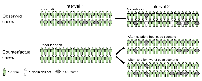
Figure 2. Illustration of a scenario where the bounds in Assumption 4 are reached. Each panel is evaluated in a stratum $A=a,L=l$. Under isolation during time interval 1, there would be 3 more individuals at risk during time interval 2 compared to the observed data with no isolation. In the best case scenario, none of the 3 individuals would develop the outcome during interval 2 after isolation. In the worst case scenario, all 3 individuals would develop the outcome during interval 2 after isolation.

Assumption 4 can be violated if there exist causal paths from $E_{1}$ to $\Delta Y_{2}$ that are not intersected by $\Delta Y_{1}$, e.g. the path $E_{1}\rightarrow\Delta Y_{2}$ in Figure 3 (A). In Appendix C, we show that Assumption 4 is implied by an exclusion restriction assumption under an intervention that prevents the outcome from occurring during time interval 1. For example, Assumption 4 can fail if isolation during time interval 1 precludes exposure to the infectious pathogen in cases where recurrent exposures contribute to sustained natural immunity without causing the outcome. In other words, Assumption 4 can fail if a substantial proportion of infections are not detected, e.g. when infections are asymptomatic. In such cases, individuals may become more susceptible to infectious exposures during time interval 2 if they are isolated during time interval 1. For example, natural immunity against severe malaria wanes over time in individuals who migrate from malaria endemic countries to non-endemic countries (Mischlinger et al., 2020). Likewise, increases in RSV infections after COVID-19 lockdown may have been caused by prolonged periods without viral exposure, reducing naturally acquired immunity (Bardsley et al., 2023). It is possible to falsify Assumption 4 by observing whether any placebo recipients develop antibodies (or other vaccine-specific immune markers) during interval 1 without experiencing the event $\Delta Y_{1}$.

Assumption 4 can also fail for other outcomes than infection. For instance, suppose that $\Delta Y_{k}$ denotes death during interval $k$. Then, an infection in time interval 1 can affect survival in time interval 2 through pathways that are not intersected by survival status during time interval 1, for example by causing serious illness and prolonged hospitalization. This would correspond to a path $E_{1}\rightarrow\Delta Y_{2}$ in Figure 3 (A).

In the COVID-19 example, an exposure that does not result in COVID-19 infection during time interval 1 is unlikely to change an individual’s contact behavior during time interval 2, corresponding to the path $E_{1}\rightarrow E_{2}\rightarrow\Delta Y_{2}$ in Figure 3 (A).

In the following example, we consider another exposure intervention.

Example (Alternative exposure intervention).

Let $E_{k}=1$ denote individuals who are free to interact in an environment where they can be exposed to the infectious agent. Conversely, define $E_{k}=0$ to mean that individuals are isolated, i.e. confined to an environment where they cannot be exposed to the infectious agent. Likewise, let $e_{k}=0$ and $e_{k}=1$ denote controlled procedures whereby individuals are isolated versus introduced into such an environment. For example, in the trial design discussed by Ray et al. (2020), individuals are vaccinated for influenza before the seasonal outbreak, and are therefore initially isolated until the seasonal outbreak begins, disregarding infections out of season. Alternatively, in a trial contrasting early versus late vaccination of individuals before travelling to areas where the infectious agent is widespread, individuals are isolated before travel, and then exposed on arrival. Under this definition of infectious exposure, being part of a population of infective individuals is viewed as an infectious challenge in itself. Thus, in the observed data described in Section 2, $E_{k}=1$ w.p. 1. Then, Assumptions 2-3 and Assumption 5 hold by design, although Assumption 4 can still fail. Furthermore, to interpret the challenge effect as a measure of vaccine protection, we still require the study environment, e.g. viral load per exposure, to be constant across intervals 1 and 2.

4. Identification

4.1. Identification assumptions

The following additional assumption, which concerns common causes of exposure and the outcome, is useful for identification of the challenge effect.

Assumption 5 (Exposure exchangeability).

For all $a,e_{1},e_{2}\in\{0,1\}$,

$$\Delta Y_{1}^{a,e_{1}},\Delta Y_{2}^{a,e_{1}}\mathchoice{\mathrel{\hbox to0.0pt{$\displaystyle\perp$\hss}\mkern 2.0mu{\displaystyle\perp}}}{\mathrel{\hbox to0.0pt{$\textstyle\perp$\hss}\mkern 2.0mu{\textstyle\perp}}}{\mathrel{\hbox to0.0pt{$\scriptstyle\perp$\hss}\mkern 2.0mu{\scriptstyle\perp}}}{\mathrel{\hbox to0.0pt{$\scriptscriptstyle\perp$\hss}\mkern 2.0mu{\scriptscriptstyle\perp}}}E_{1}^{a}\mid A=a,L\text{ and }\Delta Y_{2}^{a,e_{1},e_{2}}\mathchoice{\mathrel{\hbox to0.0pt{$\displaystyle\perp$\hss}\mkern 2.0mu{\displaystyle\perp}}}{\mathrel{\hbox to0.0pt{$\textstyle\perp$\hss}\mkern 2.0mu{\textstyle\perp}}}{\mathrel{\hbox to0.0pt{$\scriptstyle\perp$\hss}\mkern 2.0mu{\scriptstyle\perp}}}{\mathrel{\hbox to0.0pt{$\scriptscriptstyle\perp$\hss}\mkern 2.0mu{\scriptscriptstyle\perp}}}E_{2}^{a,e_{1}}\mid A=a,L\leavevmode\nobreak\ .$$

Exposure exchangeability states that exposure and the outcome are unconfounded conditional on baseline covariates. Tsiatis and Davidian (2022) used an assumption closely related to Assumption 5; they assumed that $\{\pi_{1}(t,\tau),\pi_{0}(t,\tau)\}\mathchoice{\mathrel{\hbox to0.0pt{$\displaystyle\perp$\hss}\mkern 2.0mu{\displaystyle\perp}}}{\mathrel{\hbox to0.0pt{$\textstyle\perp$\hss}\mkern 2.0mu{\textstyle\perp}}}{\mathrel{\hbox to0.0pt{$\scriptstyle\perp$\hss}\mkern 2.0mu{\scriptstyle\perp}}}{\mathrel{\hbox to0.0pt{$\scriptscriptstyle\perp$\hss}\mkern 2.0mu{\scriptscriptstyle\perp}}}\{S,c^{b}\}\mid X$, where $\pi_{a}(t,\tau)$ is the counterfactual individual-specific transmission probability per contact under treatment $A=a$, $S$ denotes a vaccination site, $X$ is a set of baseline covariates and $c^{b}$ is a contact rate.

The causal graphs in Figure 3 (A) and (B) illustrate two different data generating mechanisms violating Assumptions 3-5 by paths $A\rightarrow E_{k}$, $E_{1}\rightarrow\Delta Y_{2}$, $E_{1}\rightarrow E_{2}$ and $E_{2}^{a,e_{1}}\leftarrow U_{EY}\rightarrow\Delta Y_{2}^{a,e_{1},e_{2}}$. In contrast, the causal graph in Figure 1 satisfies Assumptions 3-5.

(a)

(b)

Figure 3. (A) The red paths $E_{1}\rightarrow\Delta Y_{2}$ and $E_{1}\rightarrow E_{2}$ can violate exposure effect restriction (Assumption 4), and the red paths $A\rightarrow E_{k}$ can violate no effect of treatment in the unexposed (Assumption 3). (B) Backdoor paths between exposure $E_{k}$ and outcome $\Delta Y_{k}$ that are not blocked by baseline covariates $L$, such as the red path $E_{2}^{a,e_{1}}\leftarrow U_{UE}\rightarrow\Delta Y_{2}^{a,e_{1},e_{2}}$, can violate exposure exchangeability (Assumption 5). However, common causes of $\Delta Y_{k}$ and $E_{k}$, such as the blue paths $\Delta Y_{1}^{a,e_{1}}\leftarrow U_{Y}\rightarrow\Delta Y_{2}^{a,e_{1},e_{2}}$ and $E_{1}^{a}\leftarrow U_{E}\rightarrow E_{2}^{a,e_{1}}$, do not violate exposure exchangeability. In the absence of $U_{E},U_{Y}$ (blue paths), $\text{VE}_{k}^{\mathrm{challenge}}=\text{VE}_{k}^{\mathrm{obs}}$ during both intervals $k\in\{1,2\}$, otherwise $\text{VE}_{2}^{\mathrm{challenge}}$ can differ from $\text{VE}_{2}^{\mathrm{obs}}$ due to depletion of susceptible individuals during time interval 1.

4.2. Identification results

In the following theorem, we give bounds on the challenge effect under the assumptions introduced so far.

Theorem 1.

Suppose that Assumptions 1-5 hold in a conventional vaccine trial (formalized in Appendix B). Then, the challenge effect during time interval 1 is point identified,

(4) $$\text{VE}_{1}^{\mathrm{challenge}}(l)=\text{VE}_{1}^{\mathrm{obs}}(l)=1-\frac{E[Y_{1}\mid A=1,L=l]}{E[Y_{1}\mid A=0,L=l]}\leavevmode\nobreak\ ,$$

whenever $E[\Delta Y_{1}\mid A=a,L=l]>0$ for all $a\in\{0,1\}$, and the challenge effect during interval 2 is partially identified by sharp bounds $\mathcal{L}_{2}(l)\leq\text{VE}_{2}^{\mathrm{challenge}}(l)\leq\mathcal{U}_{2}(l)$, where

(5) $$\mathcal{L}_{2}(l) =1-\frac{E[Y_{2}\mid A=1,L=l]}{E[Y_{2}-Y_{1}\mid A=0,L=l]}\leavevmode\nobreak\ ,$$

(6) $$\mathcal{U}_{2}(l) =1-\frac{E[Y_{2}-Y_{1}\mid A=1,L=l]}{E[Y_{2}\mid A=0,L=l]}\leavevmode\nobreak\ ,$$

whenever $E[Y_{2}-Y_{1}\mid A=a,L=l]>0$.

A proof of Theorem 1 is given in Appendix B. Additionally, in the Supplementary Material, we give R code illustrating a counterfactual data generating mechanism that attains the bounds $\mathcal{L}_{2}(l)$ and $\mathcal{U}_{2}(l)$.

The upper bound $\mathcal{U}_{2}(l)$ is reached when $i$) all the individuals that were infected during time interval 1 in the placebo arm would have become infected if they were isolated during interval 1 and challenged with the exposure during interval 2, $ii$) none of the individuals that were infected during time interval 1 in the vaccine arm would have become infected if they were isolated during interval 1 and challenged with the exposure during interval 2 and $iii$) every individual that was uninfected during interval 1 would have an unchanged outcome during interval 2 if they were isolated during interval 1. We can use a similar argument to find a scenario where the lower bound $\mathcal{L}_{2}(l)$ is reached.

It is straightforward to show that $\mathcal{L}_{2}(l)\leq\text{VE}_{2}^{\mathrm{obs}}(l)\leq\mathcal{U}_{2}(l)$ by re-expressing the bounds in Theorem 1 in terms of discrete hazards functions. If few events occur during time interval 1, it follows from Theorem 1 that the resulting bounds both approach $\text{VE}_{2}^{\mathrm{obs}}$. A heuristic observation along these lines was made by Follmann et al. (2021); Fintzi and Follmann (2021). Furthermore, Theorem 1 clarifies plausible and testable assumptions for partial identification of (challenge) vaccine waning and provides sharp bounds under the identifying assumptions.

Because $e_{k}=1$ denotes inoculation by a representative dose of the infectious agent (Assumption 1), a comparison across studies of challenge effects identified by Theorem 1 typically compares infectious inocula of different sizes that e.g. depend on the prevalence of infection in the respective background populations.

The marginal challenge effect, involving quantities $1-E[\Delta Y_{1}^{a=1,e_{1}=1}]/E[\Delta Y_{1}^{a=0,e_{1}=1}]$ and $1-E[\Delta Y_{2}^{a=1,e_{1}=0,e_{2}=1}]/E[\Delta Y_{2}^{a=0,e_{1}=0,e_{2}=1}]$, can be expressed as a weighted average over the conditional challenge effect in (1) with weights that are unidentified when exposure status $E$ is unmeasured (Stensrud and Smith, 2023; Huitfeldt et al., 2019). However, under the additional assumption that infectious exposure deterministically causes the outcome in placebo recipients, the marginal challenge effect is also point identified (Stensrud and Smith, 2023).

Proposition 1.

Suppose that Assumptions 1-5 hold in a conventional vaccine trial (formalized in Appendix B). Assume further that for all $a\in\{0,1\}$,

(7) $$\Delta Y_{2}^{a} \mathchoice{\mathrel{\hbox to0.0pt{$\displaystyle\perp$\hss}\mkern 2.0mu{\displaystyle\perp}}}{\mathrel{\hbox to0.0pt{$\textstyle\perp$\hss}\mkern 2.0mu{\textstyle\perp}}}{\mathrel{\hbox to0.0pt{$\scriptstyle\perp$\hss}\mkern 2.0mu{\scriptstyle\perp}}}{\mathrel{\hbox to0.0pt{$\scriptscriptstyle\perp$\hss}\mkern 2.0mu{\scriptscriptstyle\perp}}}E_{1}^{a}\mid\Delta Y_{1}^{a},E_{2}^{a},A=a,L\leavevmode\nobreak\ ,$$

(8) $$E_{2}^{a} \mathchoice{\mathrel{\hbox to0.0pt{$\displaystyle\perp$\hss}\mkern 2.0mu{\displaystyle\perp}}}{\mathrel{\hbox to0.0pt{$\textstyle\perp$\hss}\mkern 2.0mu{\textstyle\perp}}}{\mathrel{\hbox to0.0pt{$\scriptstyle\perp$\hss}\mkern 2.0mu{\scriptstyle\perp}}}{\mathrel{\hbox to0.0pt{$\scriptscriptstyle\perp$\hss}\mkern 2.0mu{\scriptscriptstyle\perp}}}E_{1}^{a}\mid\Delta Y_{1}^{a},A=a,L\leavevmode\nobreak\ ,$$

and that $P(E_{1}=0\mid A=a,L)>0$ and $E[\Delta Y_{2}\mid A=a,L]>0$ w.p. 1. Then,

(9) $$E[\Delta Y_{2}^{e_{1}=0}\mid A=a,L]=E[\Delta Y_{2}\mid\Delta Y_{1}=0,A=a,L]\text{ w.p. 1 }\leavevmode\nobreak\ ,$$

which implies that $\text{VE}_{2}^{\mathrm{challenge}}(l)=\text{VE}_{2}^{\mathrm{obs}}(l)$ for all $l$.

Equality (9) implies Assumption 4, and thus (7)-(8) imply Assumption 4. Furthermore, (9) is an equality involving only single world quantities (Richardson and Robins, 2013), and can therefore in principle be falsified in a future challenge trial with an immediate challenge versus isolation followed by a delayed challenge. Challenge trials will clearly be unethical to conduct in many settings, especially if recipients of the control treatment $A=0$ are vulnerable to severe infectious outcomes, but there are also many examples of such trials being conducted, see e.g.  Roestenberg et al. (2012); Killingley et al. (2022).

Expressions (7)-(8) are strong homogeneity assumptions, which can be violated by the presence of $U_{Y}$, $U_{E}$ or paths $E_{1}\rightarrow E_{2}$, $E_{1}\rightarrow\Delta Y_{2}$ in Figure 3, and are not necessary for the bounds in Theorem 1 to be informative about vaccine waning. Proposition 1 formalizes sufficient conditions under which $\text{VE}_{2}^{\mathrm{challenge}}(l)$ is identified by $\text{VE}_{2}^{\mathrm{obs}}(l)$. A special case arises when Assumptions 1-5 and (7)-(8) hold without baseline covariates; then, $\text{VE}_{k}^{\mathrm{challenge}}=\text{VE}_{k}^{\mathrm{obs}}$ marginally for all $k$, and conventional vaccine efficacy estimates are equal to the marginal challenge effect. This is an even stronger homogeneity condition, which also requires the absence of all backdoor paths $E_{k}\leftarrow L\rightarrow\Delta Y_{k}$ in Figure 3 (A). Investigators who want to quantify vaccine waning should decide on a case-by-case basis whether to report estimates of $\mathcal{L}_{2}(l),\mathcal{U}_{2}(l),\text{VE}_{2}^{\mathrm{obs}}(l)$ or marginal estimands, and justify their assumptions accordingly using subject matter knowledge. We do not rely on these homogeneity conditions in our analysis of the BNT162b2 COVID-19 vaccine trial in Section 6.

Next, suppose that the effect of placebo does not wane in the sense that the risk of the outcomes under a challenge immediately after placebo administration is equal to the risk of outcomes under isolation during interval 1, and subsequent challenge during interval 2.

Assumption 6 (No waning of placebo).

(10) $$E[\Delta Y_{1}^{a=0,e_{1}=1}\mid L]=E[\Delta Y_{2}^{a=0,e_{1}=0,e_{2}=1}\mid L]\text{ w.p.\leavevmode\nobreak\ 1}\leavevmode\nobreak\ .$$

Assumption 6 states that a controlled exposure leads to the same outcomes in conditional expectation, whether or not the exposure is preceded by an isolation period. The assumption could be violated if isolation during interval 1 leads to a loss of natural immunity against the infectious agent, but this violation is unlikely in Thomas et al. (2021) since around $95\%$ of participants had no prior history of COVID-19 infections, and we do not expect short term isolation to affect natural immunity in immunologically naive individuals.

4.3. An alternative target trial

Under no waning of placebo, it follows straightforwardly from Theorem 1 that we can bound the ratio $\psi=E[\Delta Y_{1}^{a=1,e_{1}=1}\mid L=l]/E[\Delta Y_{2}^{a=1,e_{1}=0,e_{2}=1}\mid L=l]$ by

(11) $$\mathcal{L}_{\psi}(l)\leq\psi\leq\mathcal{U}_{\psi}(l)\leavevmode\nobreak\ ,$$

where

(12) $$\mathcal{L}_{\psi}(l) =\frac{1-\text{VE}_{1}^{\mathrm{obs}}(l)}{1-\mathcal{L}_{2}(l)}\leavevmode\nobreak\ ,$$

(13) $$\mathcal{U}_{\psi}(l) =\frac{1-\text{VE}_{1}^{\mathrm{obs}}(l)}{1-\mathcal{U}_{2}(l)}\leavevmode\nobreak\ .$$

The estimand $\psi$ can also be expressed as $\psi=(1-\text{VE}_{1}^{\mathrm{challenge}}(l))/(1-\text{VE}_{2}^{\mathrm{challenge}}(l))$, and corresponds to the following target trial (Hernán et al., 2022): Let a group of individuals be randomized to one of two treatment groups on a calendar date $X$. On the same date, all individuals in both groups are vaccinated. In one treatment group, all individuals are isolated against infectious exposures until calendar date $Y$, and then they are inoculated through a controlled procedure. In the second treatment group, all individuals are vaccinated and directly inoculated with the infectious agent through the same controlled procedure. The outcome of interest is the cumulative incidence of infection during a pre-specified duration of time after calendar date $Y$, for example 2 months. If there are more outcome events under a challenge that precedes an isolation period after vaccination ($\Delta Y_{2}^{a=1,e_{1}=0,e_{2}=1}$) compared to an immediate challenge after vaccination ($\Delta Y_{1}^{a=1,e_{1}=1}$), that is, $\psi<1$, then the vaccine has waned. The target trial is similar to the estimand identified by the clinical experiment proposed by Ray et al. (2020), which is a contrast of observed incidence of influenza infection in recently vaccinated individuals versus individuals vaccinated further in the past.

Finally, under the homogeneity conditions in Proposition 1, $\psi$ is identified by the naive contrast of cumulative incidences $\psi^{\mathrm{obs}}=(1-\text{VE}_{1}^{\mathrm{obs}})/(1-\text{VE}_{2}^{\mathrm{obs}})$.

5. Estimation

Suppose we have access to data for individuals $i\in\{1,\dots,n\}$ consisting of treatment and covariates $A_{i},L_{i}$ and event times $T_{i}$ subject to losses to follow-up (censoring), indicated by $C_{i}\in\{0,1\}$. We assume that individuals are sampled into the study through a procedure such that the random vectors $(A_{i},L_{i},T_{i},C_{i})$ are i.i.d. (Cox, 1958). Then, for each treatment group $a\in\{0,1\}$, we estimate the conditional cumulative incidence functions, $E[Y_{k}\mid A=a,L=l]$, at the end of interval $k$ (time $t_{k}$) by $\widehat{\mu}_{k,a,l}=1-\exp(-\widehat{\Lambda}_{0,a}(t_{k}))^{r(l;\widehat{\beta}_{a})}$ using the Breslow estimator $\widehat{\Lambda}_{0,a}(t)$ and estimated coefficients $\widehat{\beta}_{a}$ that maximizes the partial likelihood with respect to the proportional hazards model $\lambda(t\mid A=a,L=l)=\lambda_{0,a}(t)r(l;\beta_{a})$ for $t\in[0,t_{K}]$ (Cox, 1972). Here, $\lambda_{0,a}(t)$ denotes the baseline hazard of the infectious outcome at time $t$ in treatment group $A=a$. The estimator $\widehat{\mu}_{k,a,l}$ is a standard cumulative incidence estimator (Therneau and Grambsch, 2000), and can easily be implemented using standard statistical software. We give an example in R using the survival package (Therneau, 2023) in the Supplementary Material. In our data example, we assumed that the parametric part of the hazard model is given by $r(l;\beta_{a})=\exp(\beta_{a}l)$. We chose to handle tied event times in the Cox model fit using the Efron approximation (Therneau and Grambsch, 2000). It is also possible to estimate the cumulative incidence function through other frequently used regression models, such as logistic regression, as we discuss in Appendix F, or additive hazards models (Aalen et al., 2008).

Finally, expressions (2), (4)-(6) and (12)-(13) motivate the plugin-estimators

$$\widehat{\text{VE}}_{1}^{\mathrm{obs}}(l) =1-\frac{\widehat{\mu}_{k=1,a=1,l}}{\widehat{\mu}_{k=1,a=0,l}}\leavevmode\nobreak\ ,$$

$$\widehat{\text{VE}}_{2}^{\mathrm{obs}}(l) =1-\frac{\widehat{\mu}_{k=2,a=1,l}-\widehat{\mu}_{k=1,a=1,l}}{\widehat{\mu}_{k=2,a=0,l}-\widehat{\mu}_{k=1,a=0,l}}\cdot\frac{1-\widehat{\mu}_{k=1,a=0,l}}{1-\widehat{\mu}_{k=1,a=1,l}}\leavevmode\nobreak\ ,$$

$$\widehat{\mathcal{L}}_{2}(l) =1-\frac{\widehat{\mu}_{k=2,a=1,l}}{\widehat{\mu}_{k=2,a=0,l}-\widehat{\mu}_{k=1,a=0,l}}\leavevmode\nobreak\ ,$$

$$\widehat{\mathcal{U}}_{2}(l) =1-\frac{\widehat{\mu}_{k=2,a=1,l}-\widehat{\mu}_{k=1,a=1,l}}{\widehat{\mu}_{k=2,a=0,l}}\leavevmode\nobreak\ ,$$

$$\widehat{\mathcal{L}}_{\psi}(l) =(1-\widehat{\text{VE}}_{1}^{\mathrm{obs}}(l))/(1-\widehat{\mathcal{L}}_{2}(l))\leavevmode\nobreak\ ,$$

$$\widehat{\mathcal{U}}_{\psi}(l) =(1-\widehat{\text{VE}}_{1}^{\mathrm{obs}}(l))/(1-\widehat{\mathcal{U}}_{2}(l))\leavevmode\nobreak\ .$$

Pointwise confidence intervals can, e.g., be estimated with individual-level data using non-parametric bootstrap, which we illustrate in Appendix H using a publicly available synthetic dataset resembling the RTS,S/AS01 malaria vaccine trial (RTS,S Clinical Trials Partnership, 2012), described by Benkeser et al. (2019).

Suppose a decision-maker is interested in the lower bound $\mathcal{L}_{k}(l)$, because they are concerned about the worst-case scenario corresponding to the greatest extent of waning. Then, we propose to use a lower one-sided $95\%$ confidence interval for $\widehat{\mathcal{L}}_{k}(l)$, as $\mathcal{L}_{k}(l)$ will exceed this confidence limit in 95% of cases under correctly specified assumptions. Conversely, for a decision-maker who is interested in testing whether any waning is present, we propose to use a one-sided upper $95\%$ confidence interval for $\widehat{\mathcal{U}}_{k}(l)$. Finally, decision-makers who seek to weigh the lower and upper bounds evenly may prefer to use a joint confidence for the lower and upper bound (Horowitz and Manski, 2000).

In Appendix G, we describe estimators of the bounds $\mathcal{L}_{k}$ and $\mathcal{U}_{k}$ using summary data for the number of recorded events and person time at risk. Furthermore, in Appendix I, we describe estimators of $\text{VE}_{k}^{\mathrm{obs}}$ and of bounds of $\text{VE}_{k}^{\mathrm{challenge}}$ that use logistic regression to estimate the cumulative incidences, and illustrate the approach with a simulated example.

6. Example: BNT162b2 against COVID-19

We analyzed data from a blinded, placebo controlled vaccine trial described by Thomas et al. (2021), where individuals were randomized to two doses of the mRNA vaccine BNT162b2 against COVID-19 ($A=1$) or placebo ($A=0$), 21 days apart. Participants were 12 years or older, and were enrolled during a period of time from July 27, 2020 to October 29, 2020 (older than 16) and from October 15, 2020 to January 12, 2021 (aged 12-15), in 152 sites in the United States (130 sites), Argentina (1 site), Brazil (2 sites), South Africa (4 sites), Germany (6 sites) and Turkey (9 sites). By January 12, 2021, there had been 21.94 million cases of COVID-19 in the United States (Mathieu et al., 2020), amounting to roughly 7% of the US population (United States Census Bureau, 2024). The study included systematic measures to test participants for infection with COVID-19, with 5 follow-up visits within the first 12 months, and an additional sixth follow-up visit after 24 months (Thomas et al., 2021, Protocol). Here, participants were questioned about respiratory symptoms. Additionally, they were instructed to report any respiratory symptoms via a telehealth visit after symptom onset.

Vaccine efficacy estimates ($\text{VE}^{\mathrm{obs}}$) were reported to decrease with time since vaccination (Thomas et al., 2021). In principle, the decrease of $\text{VE}^{\mathrm{obs}}$ over time could be due to declining protection of the vaccine, or alternatively also due to a higher depletion of susceptible individuals in the placebo group compared to the vaccine group during time interval 1. To distinguish between these two explanations, we conducted inference on (1) using publicly available summary data from Thomas et al. (2021), reported in Table 1. A detailed description of the estimators is given in Appendix G.

We let $k=1$ denote the time interval from 11 days after dose 1 until 2 months after dose 2, and $k=2$ to denote the time interval from 2 months after dose 2 until 4 months after dose 2 (Figure 4). Individuals received the second dose of the vaccine 10 days into interval $k=1$. The estimate $\widehat{\mathrm{VE}}^{\mathrm{challenge}}_{1}$ can be interpreted as a conservative estimate of the challenge effect if individuals had been isolated from dose 1 until shortly after dose 2 and then inoculated ($e_{1}=1$), under the assumption that vaccine protection was at its greatest shortly after dose 2. We give a detailed argument for this claim in Appendix J, and present a sensitivity analysis which does not use this assumption in Table 8 (Appendix J).

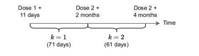
Figure 4. Illustration of time intervals $k=1$ and $k=2$

For a given interval 1, investigators face a trade-off when choosing an appropriate length of interval 2: a longer interval 2 gives narrower bounds (5)-(6), in addition to narrower confidence interval as more events are accrued. Thereby, a longer interval 2 can give a more sensitive test of vaccine waning. However, Assumption 1 is more likely to be violated if interval 2 greatly exceeds interval 1 in length, as viral loads per exposure may change over time, and the risk of multiple exposures per interval increases with a longer interval 2. This could lead the contrast of estimates $\widehat{\text{VE}}_{1}^{\mathrm{challenge}}$ vs. $\widehat{\text{VE}}_{2}^{\mathrm{challenge}}$ to compare different versions of infectious challenges if the lengths of intervals 1 and 2 differ greatly.

Table 1. Estimates and 95% confidence intervals for (2), (5)-(6) and (12)-(13). Interval 1 ranged from 11 days after dose 1 until 2 months after dose 2 (71 days in total) and interval 2 ranged from 2 months after dose 2 until 4 months after dose 2 (61 days in total). Confidence intervals for the bounds $\mathcal{L}_{\bullet},\mathcal{U}_{\bullet}$ were one-sided, whereas two-sided confidence intervals were used for VE estimates. The point estimates of $\widehat{\text{VE}}_{1}^{\mathrm{obs}},\widehat{\mathcal{U}}_{2}$ and $\widehat{\mathcal{U}}_{\psi}$ are consistent with waning vaccine protection, but the confidence intervals include the null value of no waning.

Estimand	Estimate (95% CI)
$\widehat{\text{VE}}_{1}^{\text{obs}},\widehat{\text{VE}}_{1}^{\text{challenge}}$	$0.95(0.93,0.97)$
$\widehat{\text{VE}}_{2}^{\text{obs}}$	$0.90(0.87,0.93)$
$\widehat{\mathcal{L}}_{2}$	$0.87(0.84,-)$
$\widehat{\mathcal{U}}_{2}$	$0.94(-,0.95)$
$\widehat{\mathcal{L}}_{\psi}$	$0.36(0.26,-)$
$\widehat{\mathcal{U}}_{\psi}$	$0.81(-,1.27)$

The upper confidence limit of $\widehat{\mathcal{U}}_{2}$ was close to $\widehat{\text{VE}}_{1}^{\mathrm{challenge}}$ (Table 1), although the upper confidence limit of $\widehat{\mathcal{U}}_{\psi}$ exceeded 1. In Table 7 (Appendix J), where interval 2 was extended until day 190, the upper confidence limit of $\widehat{\mathcal{U}}_{2}$ was close to the lower confidence limit of $\widehat{\text{VE}}_{1}^{\mathrm{challenge}}$. Additionally, the upper confidence limit of $\widehat{\mathcal{U}}_{\psi}$ was smaller than 1. In Table 8, we considered an additional choice of intervals to illustrate possible depletion of susceptible individuals between dose 1 and dose 2 of the vaccine, which gave wide bounds that included the null (no waning). Overall, our analyses are suggest waning vaccine protection from interval 1 to interval 2.

Our primary analysis did not condition on any baseline covariates $L$, as individual patient data were not available. To illustrate the use of estimators described in Section 5 with individual-level data, we have included an additional analysis motivated by a malaria vaccine trial in Appendix H. As a sensitivity analysis, we conducted subgroup analyses of Thomas et al. (2021) in Appendix J which show that the cumulative incidence of the outcome by the end of follow-up was nearly constant across the following baseline covariates ($L$): age over 65, Charlson Comorbidity Index category $\geq 1$ and obesity, for both vaccine and placebo treatment. Therefore, we expect that estimates $\widehat{\mathrm{VE}}_{1}^{\mathrm{obs}}(l),\widehat{\mathcal{L}}_{2}(l),\widehat{\mathcal{U}}_{2}(l)$ conditional on the baseline covariates $l$ would have been close to the marginal estimates reported in Table 1 for all baseline covariates $l$. Although we cannot guarantee the absence of residual confounding given $L$ ($U_{EY}$ in Figure 3 (B)), it is plausible that the above choice of baseline covariates $L$ is sufficient to block open backdoor paths between exposure and infection status.

Our main analysis suggests that depletion of susceptible individuals could not alone account for the decline in vaccine efficacy over time. Large real-world effectiveness studies that established waning of the BNT162b2 vaccine, such as Goldberg et al. (2021); Levin et al. (2021), were published in 2021. However, it would have been possible to estimate challenge effects (4)-(6) using preliminary trial data from the BNT162b2 vaccine trial, published already in December 2020 (Polack et al., 2020). This could have provided earlier evidence of vaccine waning. Such analyses could guide future vaccination policies during the window of time before booster trials are available.

In the Supplementary Material, we include R code to simulate a data generating mechanism that reaches the bounds in Theorem 1 for the observed data distribution. This illustrates that the bounds are sharp, i.e. that the true value of $\text{VE}_{2}^{\mathrm{challenge}}$ in the vaccine trial could lie on the bounds $\widehat{\mathcal{L}}_{2},\widehat{\mathcal{U}}_{2}$ under Assumptions 1-5.

7. Discussion

The challenge effect quantifies the vaccine waning that would be observed in a hypothetical challenge trial. Often, investigators only have access to data from a conventional randomized vaccine trial where participants are freely exposed to the infectious agent in the community. We have shown that sharp bounds on the challenge effect can be derived under plausible assumptions, and we illustrate that these bounds can confirm clinically significant waning.

Our results are broadly applicable to vaccine trials using routinely collected data and can be extended to account for treatment outcome confounding in observational vaccine studies. Furthermore, the bounds on the challenge effect can be estimated using standard statistical methods that are implemented in commonly used software packages. As illustrated in Section 6, the estimators for summary data can also be applied to re-analyze historical data from vaccine studies when individual-level data are not available, for example due to privacy concerns.

The challenge effect makes it possible to distinguish between settings where the observed vaccine efficacy diminishes solely due to depletion of susceptible individuals and settings where the vaccine protection wanes over time, and thereby addresses, and formalizes, an open problem in the analysis of vaccine trials (Halloran et al., 1997). The proposed methods can offer new empirical evidence of interest in health policy questions, for example about timing of vaccinations or booster doses.

8. Acknowledgements

This work was supported by the Swiss National Science Foundation Starting Grant called “Causal inference for infectious disease control”.

Appendix A Identification under interference

As in Tsiatis and Davidian (2022), Halloran et al. (1996), and (implicitly) in most vaccine randomized trials, we have assumed that interference between the participants in the observed trial data is negligible, such that one participant’s outcome does not depend on another participant’s treatment assignment (no interference among the participants). However, while it is often plausible that interference between the trial participants is negligible, there will often be interference in a setting where a vaccine program is rolled-out in a human population. Thus, when applying conventional estimators under i.i.d. assumptions to the trial data, we draw valid superpopulation inference in a (fictive) population with potentially limited practical relevance. Yet, we will argue that the interference is not an issue when studying the challenge effect, unlike the usual vaccine efficacy estimand ($\text{VE}^{\mathrm{obs}}$). This is because the challenge effect is insensitive to the interference that arises in most infectious disease settings.

To be explicit, consider a classical randomized vaccine trial, i.e., a trial without any controlled infectious challenges. Then, the vaccine efficacy ($\text{VE}^{\mathrm{obs}}$) in the (fictive) superpopulation with no interference will not correspond to $\text{VE}^{\mathrm{obs}}$ in a realistic target population, because there will be interference (e.g. heard immunity) between individuals in the realistic target population.

Consider now a challenge trial corresponding to (1). Then, the challenge effect in the (fictive) superpopulation with no interference would be identical to the challenge effect in the (more realistic) target population with interference, because the interference is trivial under an intervention on exposure; indeed, there is no longer any interference when the exposure to the infectious agent is controlled (fixed) for all individuals. In this sense, considering effects under interventions on exposure will often be more practically relevant.

Appendix B Identification with two time intervals

Assumption 7 (Treatment exchangeability).

For all $a,e_{1},e_{2}\in\{0,1\}$,

$$E_{1}^{a},\Delta Y_{1}^{a},\Delta Y_{1}^{a,e_{1}},E_{2}^{a,e_{1}},\Delta Y_{2}^{a},\Delta Y_{2}^{a,e_{1},e_{2}}\mathchoice{\mathrel{\hbox to0.0pt{$\displaystyle\perp$\hss}\mkern 2.0mu{\displaystyle\perp}}}{\mathrel{\hbox to0.0pt{$\textstyle\perp$\hss}\mkern 2.0mu{\textstyle\perp}}}{\mathrel{\hbox to0.0pt{$\scriptstyle\perp$\hss}\mkern 2.0mu{\scriptstyle\perp}}}{\mathrel{\hbox to0.0pt{$\scriptscriptstyle\perp$\hss}\mkern 2.0mu{\scriptscriptstyle\perp}}}A\mid L\leavevmode\nobreak\ .$$

Assumption 8 (Positivity).

$$P(A=a\mid L) >0\text{ for all }a\in\{0,1\}\leavevmode\nobreak\ \text{ w.p. 1}\leavevmode\nobreak\ .$$

Assumptions 7 and 8 hold by design when $A$ is assigned by randomization, for example in an RCT.

B.1. Proof of Theorem 1

For the first time interval,

(14) $$P(\Delta Y_{1}=1\mid A=a,L)$$

$$\stackrel{{\scriptstyle\text{Assumption \ref{ass:consistency 2 intervals}}}}{{=}} P(\Delta Y_{1}^{a}=1\mid A=a,L)$$

$$\stackrel{{\scriptstyle\text{Assumption \ref{ass: exposure necessity 2 intervals}}}}{{=}} P(\Delta Y_{1}^{a}=1,E_{1}^{a}=1\mid A=a,L)$$

$$\stackrel{{\scriptstyle\text{Assumptions \ref{ass:consistency 2 intervals} }}}{{=}} P(\Delta Y_{1}^{a,e_{1}=1}=1,E_{1}^{a}=1\mid A=a,L)$$

$$\stackrel{{\scriptstyle\text{Assumption \ref{ass: exposure exchageability 2 intevals}}}}{{=}} P(\Delta Y_{1}^{a,e_{1}=1}=1\mid A=a,L)P(E_{1}^{a}=1\mid A=a,L)$$

(15) $$\stackrel{{\scriptstyle\text{Assumptions \ref{ass: treatment exchageability 2 intevals},\ref{ass: exposure positivity 2 intervals}}}}{{=}} P(\Delta Y_{1}^{a,e_{1}=1}=1\mid L)P(E_{1}^{a}=1\mid L)\leavevmode\nobreak\ .$$

Taking the ratio of (15) for $a=1$ vs. $a=0$, and using Assumption 3 to cancel the ratio of exposure probabilities gives

$$\frac{E[\Delta Y_{1}^{a=1,e_{1}=1}\mid L]}{E[\Delta Y_{1}^{a=0,e_{1}=1}\mid L]}=\frac{E[\Delta Y_{1}\mid A=1,L]}{E[\Delta Y_{1}\mid A=0,L]}\leavevmode\nobreak\ ,$$

and therefore $\text{VE}_{1}^{\mathrm{challenge}}=\text{VE}_{1}^{\mathrm{obs}}$.

For the second time interval,

$$P(\Delta Y_{2}^{e_{1}=0}=1\mid A=a,L)$$

$$\stackrel{{\scriptstyle\text{Assumption \ref{ass:consistency 2 intervals}}}}{{=}} P(\Delta Y_{2}^{a,e_{1}=0}=1\mid A=a,L)$$

$$\stackrel{{\scriptstyle\text{Assumption \ref{ass: exposure necessity 2 intervals}}}}{{=}} P(E_{2}^{a,e_{1}=0}=1,\Delta Y_{2}^{a,e_{1}=0}=1\mid A=a,L)$$

(16) $$\stackrel{{\scriptstyle\text{Assumption \ref{ass:consistency 2 intervals}}}}{{=}} P(E_{2}^{a,e_{1}=0}=1,\Delta Y_{2}^{a,e_{1}=0,e_{2}=1}=1\mid A=a,L)$$

$$\stackrel{{\scriptstyle\text{Assumptions \ref{ass: exposure exchageability 2 intevals}}}}{{=}} P(\Delta Y_{2}^{a,e_{1}=0,e_{2}=1}=1\mid A=a,L)P(E_{2}^{a,e_{1}=0}=1\mid A=a,L)$$

(17) $$\stackrel{{\scriptstyle\text{Assumptions \ref{ass: treatment exchageability 2 intevals},\ref{ass: exposure positivity 2 intervals}}}}{{=}} P(\Delta Y_{2}^{a,e_{1}=0,e_{2}=1}=1\mid L)P(E_{2}^{a,e_{1}=0}=1\mid L)\leavevmode\nobreak\ .$$

Taking the ratio of (17) for $a=0$ vs. $a=1$ and using Assumption 4 gives

$$\frac{E[\Delta Y_{1}\mid A=1,L]}{E[\Delta Y_{1}+\Delta Y_{2}\mid A=0,L]}$$

$$\quad\leq\frac{E[\Delta Y_{2}^{a=1,e_{1}=0,e_{2}=1}\mid L]}{E[\Delta Y_{2}^{a=0,e_{1}=0,e_{2}=1}\mid L]}\cdot\frac{P(E_{2}^{a=1,e_{1}=0}=1\mid L)}{P(E_{2}^{a=0,e_{1}=0}=1\mid L)}$$

$$\qquad\leq\frac{E[\Delta Y_{1}+\Delta Y_{2}\mid A=1,L]}{E[\Delta Y_{2}\mid A=0,L]}\leavevmode\nobreak\ .$$

Finally, using Assumption 3 to cancel the ratio of exposure probabilities, we obtain

$$\frac{E[\Delta Y_{2}\mid A=1,L]}{E[\Delta Y_{1}+\Delta Y_{2}\mid A=0,L]}\leq\frac{E[\Delta Y_{2}^{a=1,e_{1}=0,e_{2}=1}\mid L]}{E[\Delta Y_{2}^{a=0,e_{1}=0,e_{2}=1}\mid L]}\leq\frac{E[\Delta Y_{1}+\Delta Y_{2}\mid A=1,L]}{E[\Delta Y_{2}\mid A=0,L]}\leavevmode\nobreak\ .$$

To establish sharpness of the bounds (5) and (6), it is sufficient to show that there exists a counterfactual data generating mechanism that attains the bounds. An example that attains the lower bound $\mathcal{L}_{2}$ is given below. We define $p_{k,a,l}=E[\Delta Y_{k}\mid A=a,L=l]$ for all $k,a,l$ and denote the observed laws of $A,L$ by $P_{A},P_{L}$ respectively.

Data generating mechanism 1.

1. $L\sim P_{L}$

2. $A\sim P_{A}$

3. $U_{Y}\sim\mathrm{Unif}[0,1]$

4. $E_{1}^{a}=E_{2}^{a,e_{1}}=1$ for all $a,e_{1}$

5. 1. $\Delta Y_{1}^{a,e_{1}=1}=I(U_{Y}\leq p_{k=1,a,L})$ for all $a$

   2. $\Delta Y_{1}^{a,e_{1}=0}=0$ for all $a$

6. 1. $\Delta Y_{2}^{a=1,e_{1}=0,e_{2}=1}=I(U_{Y}\leq p_{k=1,a=1,L}+p_{k=2,a=1,L})$

   2. $\Delta Y_{2}^{a=0,e_{1}=0,e_{2}=1}=I(p_{k=1,a=0,L}<U_{Y}\leq p_{k=1,a=0,L}+p_{k=2,a=0,L})$

   3. $\Delta Y_{2}^{a,e_{1}=1,e_{2}=1}=\Delta Y_{2}^{a,e_{1}=0,e_{2}=1}I(\Delta Y_{1}^{a,e_{1}=1}=0)$ for all $a$

   4. $\Delta Y_{2}^{a,e_{1},e_{2}=0}=0$ for all $a,e_{1}$

All other counterfactuals are understood to be recursively related to (I)-(VI) through Definition 43 of Richardson and Robins (2013), under interventions restricted to $A,E_{1}$ and $E_{2}$.

The data generating mechanism generalizes the example in Figure 2. It is straightforward to verify that Data generating mechanism 1 satisfies Assumptions 1-5 and 7-8. Furthermore, the lower bound $\mathcal{L}_{2}$ is attained since

$$E[\Delta Y_{2}^{a=1,e_{1}=0,e_{2}=1}\mid L]$$

$$= E[I(U_{Y}\leq p_{k=1,a=1,L}+p_{k=2,a=1,L})\mid L]$$

$$= p_{k=1,a=1,L}+p_{k=2,a=1,L}$$

$$= E[\Delta Y_{1}+\Delta Y_{2}\mid A=1,L]\leavevmode\nobreak\ ,$$

and

$$E[\Delta Y_{1}^{a=0,e_{1}=0,e_{2}=1}\mid L]$$

$$= E[I(p_{k=1,a=0,L}<U_{Y}\leq p_{k=1,a=0,L}+p_{k=2,a=0,L})\mid L]$$

$$= p_{k=2,a=0,L}$$

$$= E[\Delta Y_{2}\mid A=0,L]\leavevmode\nobreak\ .$$

Additionally, Data generating mechanism 1 is consistent with the observed cumulative incidences $E[\Delta Y_{k}\mid A=a,L]$ for all $a,k$, since

$$E[\Delta Y_{1}\mid A=a,L]$$

$$\stackrel{{\scriptstyle\text{Assumptions \ref{ass:consistency 2 intervals},\ref{ass: treatment exchageability 2 intevals},\ref{ass: exposure positivity 2 intervals}}}}{{=}} E[\Delta Y_{1}^{a}\mid L]$$

$$= E[\Delta Y_{1}^{a,e_{1}=1}\mid L]\text{ since }E_{1}^{a}=1\text{ w.p. 1}$$

$$= E[I(U_{Y}\leq p_{k=1,a,L})\mid L]$$

$$= p_{k=1,a,L}\leavevmode\nobreak\ ,$$

and

$$E[\Delta Y_{2}\mid A=a,L]$$

$$\stackrel{{\scriptstyle\text{Assumptions \ref{ass:consistency 2 intervals},\ref{ass: treatment exchageability 2 intevals},\ref{ass: exposure positivity 2 intervals}}}}{{=}} E[\Delta Y_{2}^{a}\mid L]$$

$$= E[\Delta Y_{2}^{a,e_{1}=1,e_{2}=1}\mid L]\text{ since }E_{1}^{a}=E_{2}^{a}=1\text{ w.p. 1}$$

$$= E[I(p_{k=1,a,L}<U_{Y}\leq p_{k=1,a,L}+p_{k=2,a,L})\mid L]$$

$$= p_{k=2,a,L}\leavevmode\nobreak\ .$$

Finally, the upper bound $\mathcal{U}_{2}$ can be reached by permuting treatment groups $a=0\leftrightarrow a=1$ in (VI) (a) and (b) of Data generating mechanism 1. An implementation of Data generating mechanism 1 in R for a simplified setting with $A\sim\mathrm{Ber}(1/2)$ and without $L$ is given in the Supplementary Material.

B.2. Proof of Proposition 1

We have that

$$P(\Delta Y_{2}=1\mid\Delta Y_{1}=0,A=a,L)$$

$$\stackrel{{\scriptstyle\text{Assumption \ref{ass:consistency 2 intervals}}}}{{=}} P(\Delta Y_{2}^{a}=1\mid\Delta Y_{1}^{a}=0,A=a,L)$$

$$\stackrel{{\scriptstyle\text{Assumption \ref{ass: exposure necessity 2 intervals}}}}{{=}} P(\Delta Y_{2}^{a}=1,E_{2}^{a}=1\mid\Delta Y_{1}^{a}=0,A=a,L)$$

$$= P(\Delta Y_{2}^{a}=1\mid E_{2}^{a}=1,\Delta Y_{1}^{a}=0,A=a,L)P(E_{2}^{a}=1\mid\Delta Y_{1}^{a}=0,A=a,L)$$

$$= P(\Delta Y_{2}^{a}=1\mid E_{1}^{a}=0,E_{2}^{a}=1,\Delta Y_{1}^{a}=0,A=a,L)$$

$$\quad\times P(E_{2}^{a}=1\mid E_{1}^{a}=0,\Delta Y_{1}^{a}=0,A=a,L)W_{Y,a}W_{E,a}$$

$$\stackrel{{\scriptstyle\text{Assumption \ref{ass: exposure necessity 2 intervals}}}}{{=}} P(\Delta Y_{2}^{a}=1\mid E_{1}^{a}=0,E_{2}^{a}=1,A=a,L)P(E_{2}^{a}=1\mid E_{1}^{a}=0,A=a,L)W_{Y,a}W_{E,a}$$

$$= P(\Delta Y_{2}^{a}=1,E_{2}^{a}=1\mid E_{1}^{a}=0,A=a,L)W_{Y,a}W_{E,a}$$

$$\stackrel{{\scriptstyle\text{Assumption \ref{ass: exposure necessity 2 intervals}}}}{{=}} P(\Delta Y_{2}^{a}=1\mid E_{1}^{a}=0,A=a,L)W_{Y,a}W_{E,a}$$

$$\stackrel{{\scriptstyle\text{Assumption \ref{ass:consistency 2 intervals}}}}{{=}} P(\Delta Y_{2}^{a,e_{1}=0}=1\mid E_{1}^{a}=0,A=a,L)W_{Y,a}W_{E,a}$$

$$\stackrel{{\scriptstyle\text{Assumption \ref{ass: exposure exchageability 2 intevals}}}}{{=}} P(\Delta Y_{2}^{a,e_{1}=0}=1\mid A=a,L)W_{Y,a}W_{E,a}$$

$$\stackrel{{\scriptstyle\text{Assumption \ref{ass:consistency 2 intervals}}}}{{=}} P(\Delta Y_{2}^{e_{1}=0}=1\mid A=a,L)W_{Y,a}W_{E,a}\leavevmode\nobreak\ ,$$

where we have defined the weights

$$W_{Y,a} =\frac{P(\Delta Y_{2}^{a}=1\mid E_{2}^{a}=1,\Delta Y_{1}^{a}=0,A=a,L)}{P(\Delta Y_{2}^{a}=1\mid E_{2}^{a}=1,\Delta Y_{1}^{a}=0,E_{1}^{a}=0,A=a,L)}\leavevmode\nobreak\ ,$$

$$W_{E,a} =\frac{P(E_{2}^{a}=1\mid\Delta Y_{1}^{a}=0,A=a,L)}{P(E_{2}^{a}=1\mid E_{1}^{a}=0,\Delta Y_{1}^{a}=0,A=a,L)}\leavevmode\nobreak\ .$$

When (7)-(8) hold, then $W_{Y,a}=W_{E,a}=1$, which implies (9). Taking the ratio of (17) for $a=1$ vs. $a=0$, and using (9),

$$\frac{E[\Delta Y_{2}^{a=1,e_{1}=0,e_{2}=1}\mid L]}{E[\Delta Y_{2}^{a=0,e_{1}=0,e_{2}=1}\mid L]}=\frac{P(\Delta Y_{2}=1\mid\Delta Y_{1}=0,A=1,L)}{P(\Delta Y_{2}=1\mid\Delta Y_{1}=0,A=0,L)}\cdot\frac{P(E_{2}^{a=0,e_{1}=0}=1\mid L)}{P(E_{2}^{a=1,e_{1}=0}=1\mid L)}$$

$$= \frac{P(\Delta Y_{2}=1\mid\Delta Y_{1}=0,A=1,L)}{P(\Delta Y_{2}=1\mid\Delta Y_{1}=0,A=0,L)}\leavevmode\nobreak\ ,$$

where we have used Assumption 3 to cancel the ratio of exposure probabilities in the final line.

Appendix C Motivation for Assumption 4

Suppose that it is possible to intervene on $\Delta Y_{1}$, for example through a form of post exposure treatment that prevents the infection from developing. Thus, we assume that Definition 43 in Richardson and Robins (2013) holds for interventions on $A,E_{1},E_{2}$ and $\Delta Y_{1}$. An example of such an intervention is antiretroviral post-exposure prophylaxis (PEP) for HIV (DeHaan et al., 2022). Next, assume the population level exclusion restriction

(18) $$P(\Delta Y_{2}^{a,e_{1}=1,\Delta y_{1}=0}=1\mid L)=P(\Delta Y_{2}^{a,e_{1}=0,\Delta y_{1}=0}=1\mid L)\text{ w.p. 1}\leavevmode\nobreak\ ,$$

which can be violated by arrows $E_{1}\rightarrow E_{2}$ or $E_{1}\rightarrow\Delta Y_{2}$ in Figure 3 (A). Then,

$$P(\Delta Y_{2}^{a}=1\mid L)$$

$$= P(\Delta Y_{1}^{a}=0,\Delta Y_{2}^{a}=1\mid L)$$

$$= P(\Delta Y_{1}^{a}=0,\Delta Y_{2}^{a,\Delta Y_{1}^{a}}=1\mid L)$$

$$= P(\Delta Y_{1}^{a}=0,\Delta Y_{2}^{a,\Delta y_{1}=0}=1\mid L)$$

$$= P(\Delta Y_{2}^{a,\Delta y_{1}=0}=1\mid L)$$

$$\quad-P(\Delta Y_{1}^{a}=1,\Delta Y_{2}^{a,\Delta y_{1}=0}=1\mid L)\leavevmode\nobreak\ .$$

We have used the recursive definition of counterfactuals (Definition 43 in Richardson and Robins (2013)) in the third line. Using the fact that

$$0\leq P(\Delta Y_{1}^{a}=1,\Delta Y_{2}^{a,\Delta y_{1}=0}=1\mid L)\leq P(\Delta Y_{1}^{a}=1\mid L)\leavevmode\nobreak\ ,$$

it follows that

$$P(\Delta Y_{2}^{a}=1\mid L)\leq P(\Delta Y_{2}^{a,\Delta y_{1}=0}=1\mid L)\leq P(\Delta Y_{1}^{a}=1\mid L)+P(\Delta Y_{2}^{a}=1\mid L)\leavevmode\nobreak\ .$$

Finally, we obtain (3) from the fact that and $P(\Delta Y_{k}^{a}=1\mid L)=P(\Delta Y_{k}=1\mid A=a,L)$ for $k\in\{1,2\}$ by Assumptions 7-8, and

$$P(\Delta Y_{2}^{a,\Delta y_{1}=0}=1\mid L)$$

$$= P(\Delta Y_{2}^{a,E_{1}^{a},\Delta y_{1}=0}=1\mid L)$$

$$\stackrel{{\scriptstyle\eqref{eq: exclusion Y intervention}}}{{=}} P(\Delta Y_{2}^{a,e_{1}=0,\Delta y_{1}=0}=1\mid L)$$

$$= P(\Delta Y_{2}^{a,e_{1}=0,\Delta Y_{1}^{a,e_{1}=0}}=1\mid L)$$

$$= P(\Delta Y_{2}^{a,e_{1}=0}=1\mid L)\leavevmode\nobreak\ .$$

The penultimate line used the fact that $P(\Delta Y_{1}^{a,e_{1}=0}=0\mid L)=1$, which holds because

$$P(\Delta Y_{1}^{a,e_{1}=0}=0\mid L)$$

$$\stackrel{{\scriptstyle\text{Assumptions \ref{ass:consistency 2 intervals},\ref{ass: treatment exchageability 2 intevals},\ref{ass: exposure positivity 2 intervals}}}}{{=}} P(\Delta Y_{1}^{a,e_{1}=0}=0\mid A=a,L)$$

$$\stackrel{{\scriptstyle\text{Assumption \ref{ass: exposure exchageability 2 intevals}}}}{{=}} P(\Delta Y_{1}^{a,e_{1}=0}=0\mid E_{1}^{a}=0,A=a,L)$$

$$= P(\Delta Y_{1}^{a,E_{1}^{a}}=0\mid E_{1}^{a}=0,A=a,L)$$

$$= P(\Delta Y_{1}^{a}=0\mid E_{1}^{a}=0,A=a,L)$$

$$\stackrel{{\scriptstyle\text{Assumption \ref{ass: exposure necessity 2 intervals}}}}{{=}} 1\leavevmode\nobreak\ .$$

C.1. Alternative motivation using cross world assumptions

Instead of (18), suppose the following cross-world equality holds:

(19) $$P(\Delta Y_{2}^{a,e_{1}=0}=1\mid\Delta Y_{1}^{a}=0,L) =P(\Delta Y_{2}^{a}=1\mid\Delta Y_{1}^{a}=0,L)\text{ w.p. 1}\leavevmode\nobreak\ .$$

The equality (19) is motivated by the following: the infectious outcome during time interval 2 would be the same in those who were naturally uninfected, regardless of whether or not they would have been isolated during time interval 1. However, this justification may be deceptively simple: the equality (19) is difficult to justify in principle because it involves a cross-world quantity on the left hand side, which is difficult to interpret. Therefore, although (19) may provide intuition for (3), we do not endorse the assumption as a sufficient justification for (3).

Expression (19) implies the single world inequality (3). To see this, we have from the laws of probability that

$$P(\Delta Y_{2}^{a,e_{1}=0}=1\mid L)$$

$$= P(\Delta Y_{2}^{a,e_{1}=0}=1\mid\Delta Y_{1}^{a}=0,L)P(\Delta Y_{1}^{a}=0\mid L)$$

$$\quad+P(\Delta Y_{2}^{a,e_{1}=0}=1\mid\Delta Y_{1}^{a}=1,L)P(\Delta Y_{1}^{a}=1\mid L)\leavevmode\nobreak\ .$$

The inequality (3) follows from substituting (19) on the right hand side, and using the inequality $0\leq P(\Delta Y_{2}^{a,e_{1}=0}=1\mid\Delta Y_{1}^{a}=1,L)\leq 1$.

Appendix D Identification with multiple versions of exposure

D.1. Identification assumptions

In this section, we establish conditions that allow identification and hypothesis testing of vaccine waning in the presence of multiple versions of treatment. Suppose that multiple versions of the observed exposure $E_{k}=1$ are present in the observed data. For example, among individuals with $E_{k}=1$, there may be subgroups that are exposed 1) more than once during interval $k$, 2) to larger (or smaller) infectious inocula per infectious exposure or 3) at different anatomical barriers, for example gastrointestinal versus respiratory mucosa. In contrast, the counterfactuals $\Delta Y_{1}^{a,e_{1}=1}$ and $\Delta Y_{2}^{a,e_{1}=0,e_{2}=1}$ refer to potential outcomes under a well-defined, controlled exposure $e_{k}=1$, e.g. by intranasal inoculation with a particular quantity of infectious inoculum, in keeping with Section 3.1. We denote the exposure version (quantity of the controlled infectious inoculum) by $q$. In this case, Assumption 1 may fail for $e_{1}=1$ or $e_{2}=1$, as there may be some individuals who would have developed the outcome under the observed exposure ($E_{k}=1$), but not under the counterfactual controlled exposure ($e_{k}=1$) or vice versa. However, throughout this section we will continue to assume that there is only one version of not being exposed, such that Assumption 1 holds whenever $e_{1}=0$ and $e_{2}=0$.

To accommodate multiple versions of the observed exposure $E_{k}=1$, we will consider a modified version $G$ of the vaccine trial described in Section 2, motivated by VanderWeele and Hernán (2013) and VanderWeele (2022). In the modified trial $G$ (Figure 5), individuals are first randomized to vaccine versus placebo, $A\in\{0,1\}$, and then to a version of infectious exposure $Q_{1},Q_{2}\in\mathcal{Q}$ during intervals 1 and 2 respectively. The support $\mathcal{Q}$ contains a collection of well-defined controlled procedures to expose individuals to infectious inocula in different ways; for example by intranasal inoculation with a pipette containing a random quantity $Q_{k}$ of infectious inoculum, drawn from a pre-specified distribution. As before, we assume that there is only one version of $Q_{k}$ where individuals are not exposed to the infectious agent, and denote this by $Q_{k}=0$. In particular, we let the intervention that assigns $q_{k}=0$ in $G$ be identical to the intervention that assigns $e_{k}=0$ in the original trial for $k\in\{1,2\}$. In the modified trial $G$, we define the exposure status $E_{k}$ to be a coarse-grained version of $Q_{k}$: for $k\in\{1,2\}$, let

(20) $$E_{k}=I(Q_{k}\neq 0)\text{ and }E_{2}^{q_{1}=0}=I(Q_{2}^{q_{1}=0}\neq 0)\leavevmode\nobreak\ .$$

To establish a relation between the modified trial $G$ and the original vaccine trial, we introduce the following assumption.

Assumption 9 (Equivalence of the modified trial $G$).

The modified trial $G$ is conducted in an identical population to the trial in Section 2, with a choice of $\mathcal{Q}$ and randomization rule for $A,Q_{1},Q_{2}$ such that

(21) $$P_{G}(A,L,E_{1},\Delta Y_{1},E_{2},\Delta Y_{2})=P(A,L,E_{1},\Delta Y_{1},E_{2},\Delta Y_{2})\leavevmode\nobreak\ ,$$

(22) $$P_{G}(A,L,E_{1},\Delta Y_{1}^{q_{1}=0},E_{2}^{q_{1}=0},\Delta Y_{2}^{q_{1}=0})=P(A,L,E_{1},\Delta Y_{1}^{e_{1}=0},E_{2}^{e_{1}=0},\Delta Y_{2}^{e_{1}=0})\leavevmode\nobreak\ ,$$

where right hand side is the distribution of the trial in Section 2.

Importantly, the original trial in Section 2 and the modified trial $G$ are not necessarily identical, but they are equivalent in the sense of Assumption 9. The equivalence assumption can fail if the controlled infectious exposure versions in $\mathcal{Q}$ are not representative of the infectious exposures in the original trial, meaning that there does not exist any randomization rules for $A,Q_{1},Q_{2}$ for controlled exposures $\mathcal{Q}$ in the trial $G$ such that $P_{G}$ satisfies (21)-(22).

Figure 5. Modified trial $G$ with exposure versions $Q_{1}$ and $Q_{2}$

(a)

(b)

Figure 6. Interventions on exposure to the infectious agent in the modified trial $G$ during interval 1 (A) and interval 2 (B)

In this section, our aim is to identify

$$\text{VE}_{1}^{\mathrm{challenge}}(l,q) =1-\frac{E_{G}[\Delta Y_{1}^{a=1,q_{1}=q}\mid L=l]}{E_{G}[\Delta Y_{1}^{a=0,q_{1}=q}\mid L=l]}\leavevmode\nobreak\ ,$$

$$\text{VE}_{2}^{\mathrm{challenge}}(l,q) =1-\frac{E_{G}[\Delta Y_{2}^{a=1,q_{1}=0,q_{2}=q}\mid L=l]}{E_{G}[\Delta Y_{2}^{a=0,q_{1}=0,q_{2}=q}\mid L=l]}\leavevmode\nobreak\ ,$$

the challenge effect under infectious exposure $q$ in trial $G$ (Figure 6), in terms of the observed distribution $P(A,L,\Delta Y_{1},\Delta Y_{2})$ in the original trial. To this end, we introduce the following assumptions.

Assumption 10 (Consistency (multiple exposure versions)).

We assume that interventions on treatment $A$ and exposures $Q_{1},Q_{2}$ are well-defined such that the following consistency conditions hold in trial $G$ for all $a\in\{0,1\}$ and $q_{1},q_{2}\in\mathcal{Q}$:

1. $\text{ if }A=a\text{ then }Q_{1}=Q_{1}^{a},Q_{2}^{q_{1}=0}=Q_{2}^{a,q_{1}=0},\Delta Y_{2}^{q_{1}=0}=\Delta Y_{2}^{a,q_{1}=0}$ ,

2. $\text{ if }A=a,Q_{1}=q_{1}\text{ then }\Delta Y_{1}=\Delta Y_{1}^{a,q_{1}}$ ,

3. $\text{ if }A=a,Q_{2}^{a,q_{1}=0}=q_{2}\text{ then }\Delta Y_{2}^{a,q_{1}=0}=\Delta Y_{2}^{a,q_{1}=0,q_{2}}$ .

Assumption 11 (Treatment exchangeability (multiple exposure versions)).

For all $q_{1},q_{2}\in\mathcal{Q}$,

$$\Delta Y_{1}^{a,q_{1}},\Delta Y_{2}^{a,q_{1},q_{2}}\mathchoice{\mathrel{\hbox to0.0pt{$\displaystyle\perp$\hss}\mkern 2.0mu{\displaystyle\perp}}}{\mathrel{\hbox to0.0pt{$\textstyle\perp$\hss}\mkern 2.0mu{\textstyle\perp}}}{\mathrel{\hbox to0.0pt{$\scriptstyle\perp$\hss}\mkern 2.0mu{\scriptstyle\perp}}}{\mathrel{\hbox to0.0pt{$\scriptscriptstyle\perp$\hss}\mkern 2.0mu{\scriptscriptstyle\perp}}}A\mid L\leavevmode\nobreak\ .$$

Assumption 12 (Exposure exchangeability (multiple exposure versions)).

For all $a\in\{0,1\}$ and $q_{1},q_{2}\in\mathcal{Q}$,

$$\Delta Y_{1}^{a,q_{1}},\Delta Y_{2}^{a,q_{1}}\mathchoice{\mathrel{\hbox to0.0pt{$\displaystyle\perp$\hss}\mkern 2.0mu{\displaystyle\perp}}}{\mathrel{\hbox to0.0pt{$\textstyle\perp$\hss}\mkern 2.0mu{\textstyle\perp}}}{\mathrel{\hbox to0.0pt{$\scriptstyle\perp$\hss}\mkern 2.0mu{\scriptstyle\perp}}}{\mathrel{\hbox to0.0pt{$\scriptscriptstyle\perp$\hss}\mkern 2.0mu{\scriptscriptstyle\perp}}}Q_{1}^{a}\mid A=a,L\leavevmode\nobreak\ ,\text{ and }\Delta Y_{2}^{a,q_{1},q_{2}}\mathchoice{\mathrel{\hbox to0.0pt{$\displaystyle\perp$\hss}\mkern 2.0mu{\displaystyle\perp}}}{\mathrel{\hbox to0.0pt{$\textstyle\perp$\hss}\mkern 2.0mu{\textstyle\perp}}}{\mathrel{\hbox to0.0pt{$\scriptstyle\perp$\hss}\mkern 2.0mu{\scriptstyle\perp}}}{\mathrel{\hbox to0.0pt{$\scriptscriptstyle\perp$\hss}\mkern 2.0mu{\scriptscriptstyle\perp}}}Q_{2}^{a,q_{1}}\mid A=a,L\leavevmode\nobreak\ .$$

Assumption 13 (No waning of placebo (multiple exposure versions)).

For all $q\in\mathcal{Q}$,

$$E_{G}[\Delta Y_{1}^{a=0,q_{1}=q}\mid L]=E_{G}[\Delta Y_{2}^{a=0,q_{1}=0,q_{2}=q}\mid L]\text{ w.p.\leavevmode\nobreak\ 1}\leavevmode\nobreak\ .$$

Assumption 14 (Stationarity of exposure versions among the exposed).

For all $a\in\{0,1\}$ and $q\in\mathcal{Q}$,

$$P_{G}(Q_{1}\leq q\mid E_{1}=1,A=a,L)=P_{G}(Q_{2}^{q_{1}=0}\leq q\mid E_{2}^{q_{1}=0}=1,A=a,L)\text{ w.p.\leavevmode\nobreak\ 1}\leavevmode\nobreak\ .$$

Assumption 14 is closely related to the “Similar Study Environment” assumption by Fintzi and Follmann (2021):

“The proportional hazards model allows for the attack rate to change with time. But if the pathogen mutates to a form that is resistant to vaccine effects, efficacy may appear to wane. Another possibility is if human behavior changes in such a way that the vaccine is less effective. For example, if there is less mask wearing in the community over the study, the viral inoculum at infection may increase over the study and overwhelm the immune response for later cases. Vaccines may work less well against larger inoculums and thus VE might appear to wane. For viral mutation, analyses could be run separately for different major strains provided they occur both prior and post crossover.”

An assumption such as Assumption 14 or the Similar Study Environment assumption seems to be a bare minimum needed to identify waning using cumulative incidences of the infectious event; without such an assumption one cannot discern whether changes in cumulative incidences over time are due to changes in the exposure versions or changes in the challenge effect, as also alluded to in the quote from Fintzi and Follmann (2021). In particular, this consideration also applies to conventional approaches to vaccine waning, i.e. the direct comparison of $\text{VE}_{1}^{\mathrm{obs}}$ vs. $\text{VE}_{2}^{\mathrm{obs}}$ as considered by e.g. Fintzi and Follmann (2021). Assumption 14 does not require that the same number of individuals are exposed during intervals 1 and 2. In other words, the assumption is not necessarily violated if $P(E_{1}=1\mid L)<P(E_{2}=1\mid L)$, e.g. if the prevalence of infection increases in the larger population that embeds the trial participants. For instance, in an all-or-nothing model of vaccine protection (Halloran et al., 2012), immune individuals will never contract infection, regardless of the number of exposures during a given time interval, and those who are not immune will always contract infection if exposed. However, in a leaky model of vaccine protection, individuals with multiple exposures during interval $k$ will have a greater risk of the outcome than an individual with a single exposure. If $P(E_{1}=1\mid L)\ll P(E_{2}=1\mid L)$ w.p. 1, e.g. due to a large difference in the lengths of intervals $k=1$ vs. $k=2$, or due to a large change in the infection prevalence, then multiple exposures are more likely during interval 2 compared to 1, which could violate Assumption 14.

If one compares the incidence of recent versus early vacinees during the same interval of calendar time, as suggested by Lipsitch et al. (2019), then Assumption 14 is particularly plausible in the blinded crossover trial discussed by Follmann et al. (2021), where individuals are randomly assigned to vaccine versus control at baseline, and then cross over to the other treatment arm after a pre-specified interval of time.

To state the next assumption, we the define the dose-response relations $\varphi_{k}(q)$ and an auxiliary function $h$.

$$\varphi_{1}(q) =E[\Delta Y_{1}^{a=1,q_{1}=q}\mid L=l]\leavevmode\nobreak\ ,$$

$$\varphi_{2}(q) =E[\Delta Y_{2}^{a=1,q_{1}=0,q_{2}=q}\mid L=l]\leavevmode\nobreak\ ,$$

$$h(q) =\frac{\varphi_{1}(q)}{E_{G}[\varphi_{1}(Q_{1})\mid E_{1}=1,A=1,L=l]}-\frac{\varphi_{2}(q)}{E_{G}[\varphi_{2}(Q_{1})\mid E_{1}=1,A=1,L=l]}\leavevmode\nobreak\ .$$

Assumption 15 (Existence of a representative exposure (weak)).

There exists a representative exposure $q_{l}^{\ast}\in\mathcal{Q}$ such that

$$h(q_{l}^{\ast})=0\leavevmode\nobreak\ .$$

Since $E_{G}[h(Q_{1})\mid E_{1}=1,A=1,L=l]=0$, Assumption 15 is implied by the mean value theorem for a non-trivial class of dose-response relations $\varphi_{k}(q)$ and distributions of $Q_{k}$.

Assumption 16 (Existence of a representative exposure (strong)).

There exists a representative exposure $q_{l}^{\ast\ast}\in\mathcal{Q}$ such that

(23) $$E_{G}[\Delta Y_{1}^{a,q_{1}=q_{l}^{\ast\ast}}\mid L=l] =E_{G}[E_{G}[\Delta Y_{1}^{a,Q_{1}}\mid L=l]\mid E_{1}=1,A=a,L=l]\leavevmode\nobreak\ ,$$

(24) $$E_{G}[\Delta Y_{2}^{a,q_{1}=0,q_{2}=q_{l}^{\ast\ast}}\mid L=l] =E_{G}[E_{G}[\Delta Y_{2}^{a,q_{1}=0,Q_{2}^{q_{1}=0}}\mid L=l]\mid E_{2}^{q_{1}=0}=1,A=a,L=l]\leavevmode\nobreak\ ,$$

for all $a\in\{0,1\}$.

Assumption 16 can be regarded as a consistency assumption in conditional expectation, and states that an infectious inoculum of version $q_{l}^{\ast\ast}$ leads to the same outcome in conditional expectation as an average over a random version $Q_{1}$ among individuals with $E_{1}=1$, and likewise for a random version $Q_{2}^{q_{1}=0}$ among individuals with $E_{2}^{q_{1}=0}=1$. In other words, individuals with $Q_{1}>q_{l}^{\ast\ast}$ are perfectly balanced by individuals with $Q_{1}<q_{l}^{\ast\ast}$, for both treatment groups $A\in\{0,1\}$, and correspondingly for the second time interval. One scenario where this happens is if the conditional distribution of $Q_{1},Q_{2}^{q_{1}=0}$ is narrow and centers around the particular version $q_{l}^{\ast\ast}$. Then, only one version of the treatment occurs effectively. This is equivalent to the statement that the dose-response relations $E_{G}[\Delta Y_{1}^{a,q}\mid L=l]$ and $E_{G}[\Delta Y_{2}^{a,q_{1}=0,q_{2}=q}\mid L=l]$, viewed as functions of $q$, do not vary in $q$ over the range of treatment versions with non-negligible probability, i.e. that all the observed exposure versions lead to the same outcomes in conditional expectation. This occurs in an all-or-nothing model of vaccine protection, but not necessarily in a leaky model (Halloran et al., 2012).

D.2. Identification results

Proposition 2.

Under Assumptions 1 (i) and (ii) for $e_{1}=0$ and Assumptions 8-12,

(25) $$E[\Delta Y_{1}^{a}\mid E_{1}^{a}=1,A=a,L=l]=E_{G}[E_{G}[\Delta Y_{1}^{a,Q_{1}}\mid L=l]\mid E_{1}=1,A=a,L=l]\leavevmode\nobreak\ ,$$

$$E[\Delta Y_{2}^{a,e_{1}=0}\mid E_{2}^{a,e_{1}=0}=1,A=a,L=l]$$

(26) $$\quad=E_{G}[E_{G}[\Delta Y_{2}^{a,q_{1}=0,Q_{2}^{q_{1}=0}}\mid L=l]\mid E_{2}^{q_{1}=0}=1,A=a,L=l]\leavevmode\nobreak\ .$$

Under the additional Assumptions 2-4 and Assumption 7,

(27) $$1-\frac{E_{G}[E_{G}[\Delta Y_{1}^{a=1,Q_{1}}\mid L=l]\mid E_{1}=1,A=1,L=l]}{E_{G}[E_{G}[\Delta Y_{1}^{a=0,Q_{1}}\mid L=l]\mid E_{1}=1,A=0,L=l]} =\text{VE}_{1}^{\mathrm{obs}}(l)\leavevmode\nobreak\ ,$$

(28) $$1-\frac{E_{G}[E_{G}[\Delta Y_{2}^{a=1,q_{1}=0,Q_{2}^{q_{1}=0}}\mid L=l]\mid E_{2}^{q_{1}=0}=1,A=1,L=l]}{E_{G}[E_{G}[\Delta Y_{2}^{a=0,q_{1}=0,Q_{2}^{q_{1}=0}}\mid L=l]\mid E_{2}^{q_{1}=0}=1,A=0,L=l]} \in[\mathcal{L}_{2}(l),\mathcal{U}_{2}(l)]\leavevmode\nobreak\ .$$

Proof.

Expression (25) follows from

$$E[\Delta Y_{1}^{a}\mid E_{1}^{a}=1,A=a,L]$$

$$\stackrel{{\scriptstyle\text{Assumption\leavevmode\nobreak\ \ref{ass:consistency 2 intervals}\leavevmode\nobreak\ (i)}}}{{=}} E[\Delta Y_{1}\mid E_{1}=1,A=a,L]$$

$$\stackrel{{\scriptstyle\text{Assumption\leavevmode\nobreak\ \ref{ass:equivalence_modified_trial}}}}{{=}} E_{G}[\Delta Y_{1}\mid E_{1}=1,A=a,L]$$

$$= E_{G}[E_{G}[\Delta Y_{1}\mid Q_{1},E_{1}=1,A=a,L]\mid E_{1}=1,A=a,L]$$

$$\stackrel{{\scriptstyle\eqref{eq: Ek definition}}}{{=}} E_{G}[E_{G}[\Delta Y_{1}\mid Q_{1},A=a,L]\mid E_{1}=1,A=a,L]$$

$$\stackrel{{\scriptstyle\text{Assumption\leavevmode\nobreak\ \ref{ass:consistency_multiple_versions}}}}{{=}} E_{G}[E_{G}[\Delta Y_{1}^{a,Q_{1}^{a}}\mid Q_{1}^{a},A=a,L]\mid E_{1}=1,A=a,L]$$

$$\stackrel{{\scriptstyle\text{Assumption\leavevmode\nobreak\ \ref{ass: exposure exchageability multiple versions}}}}{{=}} E_{G}[E_{G}[\Delta Y_{1}^{a,Q_{1}^{a}}\mid A=a,L]\mid E_{1}=1,A=a,L]$$

$$\stackrel{{\scriptstyle\text{Assumption\leavevmode\nobreak\ \ref{ass: treatment exch multiple versions}}}}{{=}} E_{G}[E_{G}[\Delta Y_{1}^{a,Q_{1}^{a}}\mid L]\mid E_{1}=1,A=a,L]$$

$$\stackrel{{\scriptstyle\text{Assumption\leavevmode\nobreak\ \ref{ass:consistency_multiple_versions}\leavevmode\nobreak\ (i)}}}{{=}} E_{G}[E_{G}[\Delta Y_{1}^{a,Q_{1}}\mid L]\mid E_{1}=1,A=a,L]\leavevmode\nobreak\ .$$

The penultimate equality used the positivity condition $P_{G}(A=a\mid L)>0$ for all $a\in\{0,1\}$ w.p. 1, which follows from Assumption 8 and definition of the trial $G$ (Assumption 9). Likewise, (26) follows from

$$E[\Delta Y_{2}^{a,e_{1}=0}\mid E_{2}^{a,e_{1}=0}=1,A=a,L]$$

$$\stackrel{{\scriptstyle\text{Assumption\leavevmode\nobreak\ \ref{ass:consistency 2 intervals}\leavevmode\nobreak\ (i)}}}{{=}} E[\Delta Y_{2}^{e_{1}=0}\mid E_{2}^{e_{1}=0}=1,A=a,L]$$

$$\stackrel{{\scriptstyle\text{Assumption\leavevmode\nobreak\ \ref{ass:equivalence_modified_trial}}}}{{=}} E_{G}[\Delta Y_{2}^{q_{1}=0}\mid E_{2}^{q_{1}=0}=1,A=a,L]$$

$$= E_{G}[E_{G}[\Delta Y_{2}^{q_{1}=0}\mid Q_{2}^{q_{1}=0},E_{2}^{q_{1}=0}=1,A=a,L]\mid E_{2}^{q_{1}=0}=1,A=a,L]$$

$$\stackrel{{\scriptstyle\eqref{eq: Ek definition}}}{{=}} E_{G}[E_{G}[\Delta Y_{2}^{q_{1}=0}\mid Q_{2}^{q_{1}=0},A=a,L]\mid E_{2}^{q_{1}=0}=1,A=a,L]$$

$$\stackrel{{\scriptstyle\text{Assumption\leavevmode\nobreak\ \ref{ass:consistency_multiple_versions}}}}{{=}} E_{G}[E_{G}[\Delta Y_{2}^{a,q_{1}=0,Q_{2}^{a,q_{1}=0}}\mid Q_{2}^{a,q_{1}=0},A=a,L]\mid E_{2}^{q_{1}=0}=1,A=a,L]$$

$$\stackrel{{\scriptstyle\text{Assumption\leavevmode\nobreak\ \ref{ass: exposure exchageability multiple versions}}}}{{=}} E_{G}[E_{G}[\Delta Y_{2}^{a,q_{1}=0,Q_{2}^{a,q_{1}=0}}\mid A=a,L]\mid E_{2}^{q_{1}=0}=1,A=a,L]$$

$$\stackrel{{\scriptstyle\text{Assumption\leavevmode\nobreak\ \ref{ass: treatment exch multiple versions}}}}{{=}} E_{G}[E_{G}[\Delta Y_{2}^{a,q_{1}=0,Q_{2}^{a,q_{1}=0}}\mid L]\mid E_{2}^{q_{1}=0}=1,A=a,L]$$

$$\stackrel{{\scriptstyle\text{Assumption\leavevmode\nobreak\ \ref{ass:consistency_multiple_versions}\leavevmode\nobreak\ (i)}}}{{=}} E_{G}[E_{G}[\Delta Y_{2}^{a,q_{1}=0,Q_{2}^{q_{1}=0}}\mid L]\mid E_{2}^{q_{1}=0}=1,A=a,L]\leavevmode\nobreak\ .$$

In the first and second lines, we have used that quantities under intervention $e_{1}=0$ are well-defined, which follows from Assumption 1 (ii) for $e_{1}=0$.

We proceed similarly to Section B.1.

$$\frac{E[\Delta Y_{1}^{a=1}\mid E_{1}^{a=1}=1,A=1,L]}{E[\Delta Y_{1}^{a=0}\mid E_{1}^{a=0}=1,A=0,L]}$$

$$= \frac{E[I(E_{1}^{a=1}=1)\Delta Y_{1}^{a=1}\mid A=1,L]}{E[I(E_{1}^{a=0}=1)\Delta Y_{1}^{a=0}\mid A=0,L]}\times\frac{P(E_{1}^{a=0}=1\mid A=0,L)}{P(E_{1}^{a=1}=1\mid A=1,L)}$$

$$\stackrel{{\scriptstyle\text{Assumptions\leavevmode\nobreak\ \ref{ass: treatment exchageability 2 intevals}, \ref{ass: exposure positivity 2 intervals}}}}{{=}} \frac{E[I(E_{1}^{a=1}=1)\Delta Y_{1}^{a=1}\mid A=1,L]}{E[I(E_{1}^{a=0}=1)\Delta Y_{1}^{a=0}\mid A=0,L]}\times\frac{P(E_{1}^{a=0}=1\mid L)}{P(E_{1}^{a=1}=1\mid L)}$$

$$\stackrel{{\scriptstyle\text{Assumption\leavevmode\nobreak\ \ref{ass:no effect on exposure 2 intervals}}}}{{=}} \frac{E[I(E_{1}^{a=1}=1)\Delta Y_{1}^{a=1}\mid A=1,L]}{E[I(E_{1}^{a=0}=1)\Delta Y_{1}^{a=0}\mid A=0,L]}$$

$$\stackrel{{\scriptstyle\text{Assumption\leavevmode\nobreak\ \ref{ass: exposure necessity 2 intervals}}}}{{=}} \frac{E[\Delta Y_{1}^{a=1}\mid A=1,L]}{E[\Delta Y_{1}^{a=0}\mid A=0,L]}$$

(29) $$\stackrel{{\scriptstyle\text{Assumptions\leavevmode\nobreak\ \ref{ass:consistency 2 intervals}\leavevmode\nobreak\ (i)}}}{{=}} \frac{E[\Delta Y_{1}\mid A=1,L]}{E[\Delta Y_{1}\mid A=0,L]}\leavevmode\nobreak\ ,$$

and

$$\frac{E[\Delta Y_{2}^{a=1,e_{1}=0}\mid E_{2}^{a=1,e_{1}=0}=1,A=1,L]}{E[\Delta Y_{2}^{a=0,e_{1}=0}\mid E_{2}^{a=0,e_{1}=0}=1,A=0,L]}$$

$$= \frac{E[I(E_{2}^{a=1,e_{1}=0}=1)\Delta Y_{2}^{a=1,e_{1}=0}\mid A=1,L]}{E[I(E_{2}^{a=0,e_{1}=0}=1)\Delta Y_{2}^{a=0,e_{1}=0}\mid A=0,L]}\times\frac{P(E_{2}^{a=0,e_{1}=0}=1\mid A=0,L)}{P(E_{2}^{a=1,e_{1}=0}=1\mid A=1,L)}$$

$$\stackrel{{\scriptstyle\text{Assumptions\leavevmode\nobreak\ \ref{ass: treatment exchageability 2 intevals}, \ref{ass: exposure positivity 2 intervals}}}}{{=}} \frac{E[I(E_{2}^{a=1,e_{1}=0}=1)\Delta Y_{2}^{a=1,e_{1}=0}\mid A=1,L]}{E[I(E_{2}^{a=0,e_{1}=0}=1)\Delta Y_{2}^{a=0,e_{1}=0}\mid A=0,L]}\times\frac{P(E_{2}^{a=0,e_{1}=0}=1\mid L)}{P(E_{2}^{a=1,e_{1}=0}=1\mid L)}$$

$$\stackrel{{\scriptstyle\text{Assumption\leavevmode\nobreak\ \ref{ass:no effect on exposure 2 intervals}}}}{{=}} \frac{E[I(E_{2}^{a=1,e_{1}=0}=1)\Delta Y_{2}^{a=1,e_{1}=0}\mid A=1,L]}{E[I(E_{2}^{a=0,e_{1}=0}=1)\Delta Y_{2}^{a=0,e_{1}=0}\mid A=0,L]}$$

$$\stackrel{{\scriptstyle\text{Assumption\leavevmode\nobreak\ \ref{ass: exposure necessity 2 intervals}}}}{{=}} \frac{E[\Delta Y_{2}^{a=1,e_{1}=0}\mid A=1,L]}{E[\Delta Y_{2}^{a=0,e_{1}=0}\mid A=0,L]}$$

(30) $$\stackrel{{\scriptstyle\text{Assumption\leavevmode\nobreak\ \ref{ass:consistency 2 intervals}\leavevmode\nobreak\ (i)}}}{{=}} \frac{E[\Delta Y_{2}^{e_{1}=0}\mid A=1,L]}{E[\Delta Y_{2}^{e_{1}=0}\mid A=0,L]}$$

(31) $$\stackrel{{\scriptstyle\text{Assumption\leavevmode\nobreak\ \ref{ass: exclusion 2 intervals}}}}{{\in}} \left[\frac{E[\Delta Y_{2}\mid A=1,L]}{E[\Delta Y_{1}+\Delta Y_{2}\mid A=0,L]},\frac{E[\Delta Y_{1}+\Delta Y_{2}\mid A=1,L]}{E[\Delta Y_{2}\mid A=0,L]}\right]\leavevmode\nobreak\ .$$

Combining (25) and (29) gives (27). Likewise, (26) and (31) imply (28). ∎

Expressions (25)-(26) state that the conditional exposure risk among the exposed is equal to a marginalization of the dose-response relations $\varphi_{1}(Q_{1})$ and $\varphi(Q_{2}^{q_{1}=0})$ over random exposure versions $Q_{1}$ and $Q_{2}^{q_{1}=0}$. Thus, (27)-(28) allows us to interpret (4) and (5)-(6) as identification formulas for a randomized exposure intervention, where an investigator draws a version $Q_{1}$ and $Q_{2}^{q_{1}=0}$ at random according to the conditional distribution functions $F_{Q_{1}\mid E_{1}=1,A=a,L=l}$ and $F_{Q_{2}^{q_{1}=0}\mid E_{2}^{q_{1}=0}=1,A=a,L=l}$. However, a contrast of (27) vs. (28) could be non-null due to changes in exposure versions over time, unless Assumptions 14 holds.

Let $\mathrm{H}_{0}$ be the strict null hypothesis that the vaccine does not wane for any exposure version $q\in\mathcal{Q}$,

$$\mathrm{H}_{0}:\leavevmode\nobreak\ E[\Delta Y_{1}^{a=1,q_{1}=q}\mid L]=E[\Delta Y_{2}^{a=1,q_{1}=0,q_{2}=q}\mid L]\text{ w.p.\leavevmode\nobreak\ 1 for all }q\in\mathcal{Q}\leavevmode\nobreak\ .$$

Proposition 3.

Under Assumptions 1 (i) and (ii) for $e_{1}=0$, Assumptions 2-4 and Assumptions 7-14,

(32) $$\mathrm{H}_{0}\implies\mathcal{L}_{\psi}(l)\leq 1\leq\mathcal{U}_{\psi}(l)\leavevmode\nobreak\ .$$

Proof.

Evaluating the ratio of (25) and (26) for $a=0$, and using Assumptions 13 and 14, gives

(33) $$\frac{E[\Delta Y_{1}^{a=0}\mid E_{1}^{a=0}=1,A=0,L]}{E[\Delta Y_{2}^{a=0,e_{1}=0}\mid E_{2}^{a=0,e_{1}=0}=1,A=0,L]}=1\leavevmode\nobreak\ .$$

Similarly, by evaluating the ratio of (25) and (26) for $a=1$ under $\mathrm{H}_{0}$ and Assumption 14, we find that

(34) $$\frac{E[\Delta Y_{1}^{a=1}\mid E_{1}^{a=1}=1,A=1,L]}{E[\Delta Y_{2}^{a=1,e_{1}=0}\mid E_{2}^{a=1,e_{1}=0}=1,A=1,L]}=1\leavevmode\nobreak\ .$$

Taking the ratio of (33) and (34) gives

(35) $$1= \frac{\frac{E[\Delta Y_{2}^{a=1,e_{1}=0}\mid E_{2}^{a=1,e_{1}=0}=1,A=1,L]}{E[\Delta Y_{2}^{a=0,e_{1}=0}\mid E_{2}^{a=0,e_{1}=0}=1,A=0,L]}}{\frac{E[\Delta Y_{1}^{a=1}\mid E_{1}^{a=1}=1,A=1,L]}{E[\Delta Y_{1}^{a=0}\mid E_{1}^{a=0}=1,A=0,L]}}\leavevmode\nobreak\ .$$

Using (29) and (31) in (35) gives the final result. ∎

By testing whether the observed data violates (32), one can test the null hypothesis $\mathrm{H}_{0}$. Proposition 3 clarifies that it is possible to test for the presence of vaccine waning even under arbitrary distributions of versions of treatment, as long as the distribution is stationary over time. A violation of $\mathrm{H}_{0}$ implies that there exists at least one infectious inoculum $q$ for which the vaccine wanes, but it does not establish for which inocula $q$ the vaccine wanes. However, it would be surprising if $\text{VE}_{1}^{\mathrm{challenge}}(l,q)>\text{VE}_{2}^{\mathrm{challenge}}(l,q)$ for some $q$ while $\text{VE}_{1}^{\mathrm{challenge}}(l,q)<\text{VE}_{2}^{\mathrm{challenge}}(l,q)$ for other versions $q$, and therefore a violation of $\mathrm{H}_{0}$ gives meaningful insight into vaccine waning, even though it does not tell us by how much the vaccine wanes for each exposure version $q$. Furthermore, the power to reject $\mathrm{H}_{0}$ is driven by exposure versions that appear frequently, or wane substantially, in the observed data, and therefore a rejection of $\mathrm{H}_{0}$ gives insight on waning of such exposure versions.

In the following propositions, we clarify conditions which allow us to interpret previous identification results for $\text{VE}_{1}^{\mathrm{challenge}}$ and $\text{VE}_{2}^{\mathrm{challenge}}$ in terms of controlled exposures to non-random, representative infectious inocula.

Let $\psi(l,q)=E_{G}[\Delta Y_{1}^{a=1,q_{1}=q}\mid L=l]/E_{G}[\Delta Y_{2}^{a=1,q_{1}=0,q_{2}=q}\mid L=l]$.

Proposition 4.

Under Assumptions 1 (i) and (ii) for $e_{1}=0$, Assumptions 2-4 and Assumptions 7-15, $\mathcal{L}_{\psi}(l)\leq\psi(l,q^{\ast})\leq\mathcal{U}_{\psi}(l)$.

Proof.

Multiplying both sides of (29) by $E_{G}[\Delta Y_{1}^{a=1,q_{1}=q}\mid L]/E_{G}[\Delta Y_{1}^{a=0,q_{1}=q}\mid L]$ and both sides of (30) by $E_{G}[\Delta Y_{2}^{a=1,q_{1}=0,q_{2}=q}\mid L]/E_{G}[\Delta Y_{2}^{a=0,q_{1}=0,q_{2}=q}\mid L]$ gives

(36) $$\scriptstyle\frac{P_{G}(\Delta Y_{1}^{a=1,q_{1}=q}=1\mid L)}{P_{G}(\Delta Y_{1}^{a=0,q_{1}=q}=1\mid L)} =\scriptstyle\frac{P(\Delta Y_{1}=1\mid A=1,L)}{P(\Delta Y_{1}=1\mid A=0,L)}\times\frac{\frac{P_{G}(\Delta Y_{1}^{a=1,q_{1}=q}=1\mid L)}{P(\Delta Y_{1}^{a=1}=1\mid E_{1}^{a=1}=1,A=1,L)}}{\frac{P_{G}(\Delta Y_{1}^{a=0,q_{1}=q}=1\mid L)}{P(\Delta Y_{1}^{a=0}=1\mid E_{1}^{a=0}=1,A=0,L)}}\leavevmode\nobreak\ ,$$

(37) $$\scriptstyle\frac{P_{G}(\Delta Y_{2}^{a=1,q_{1}=0,q_{2}=q}=1\mid L)}{P_{G}(\Delta Y_{2}^{a=0,q_{1}=0,q_{2}=q}=1\mid L)} =\scriptstyle\frac{P(\Delta Y_{2}^{e_{1}=0}=1\mid A=1,L)}{P(\Delta Y_{2}^{e_{1}=0}=1\mid A=0,L)}\times\frac{\frac{P_{G}(\Delta Y_{2}^{a=1,q_{1}=0,q_{2}=q}=1\mid L)}{P(\Delta Y_{2}^{a=1,e_{1}=0}=1\mid E_{2}^{a=1,e_{1}=0}=1,A=1,L)}}{\frac{P_{G}(\Delta Y_{2}^{a=0,q_{1}=0,q_{2}=q}=1\mid L)}{P(\Delta Y_{2}^{a=0,e_{1}=0}=1\mid E_{2}^{a=0,e_{1}=0}=1,A=0,L)}}\leavevmode\nobreak\ .$$

Assumptions 14 and 15 together imply that

(38) $$\scriptstyle\frac{P_{G}(\Delta Y_{1}^{a=1,q_{1}=q_{l}^{\ast}}=1\mid L)}{E_{G}[E_{G}[\Delta Y_{1}^{a=1,Q_{1}}\mid L]\mid E_{1}=1,A=1,L]}=\scriptstyle\frac{P_{G}(\Delta Y_{2}^{a=1,q_{1}=0,q_{2}=q_{l}^{\ast}}=1\mid L)}{E_{G}[E_{G}[\Delta Y_{2}^{a=1,q_{1}=0,Q_{2}^{q_{1}=0}}\mid L]\mid E_{2}^{q_{1}=0}=1,A=1,L]}\leavevmode\nobreak\ .$$

Next, Assumptions 13 and 14 imply that

(39) $$\scriptstyle\frac{P_{G}(\Delta Y_{1}^{a=0,q_{1}=q_{l}^{\ast}}=1\mid L)}{E_{G}[E_{G}[\Delta Y_{1}^{a=0,Q_{1}}\mid L]\mid E_{1}=1,A=0,L]}=\scriptstyle\frac{P_{G}(\Delta Y_{2}^{a=0,q_{1}=0,q_{2}=q_{l}^{\ast}}=1\mid L)}{E_{G}[E_{G}[\Delta Y_{2}^{a=0,q_{1}=0,Q_{2}^{q_{1}=0}}\mid L]\mid E_{2}^{q_{1}=0}=1,A=0,L]}\leavevmode\nobreak\ .$$

Taking the ratio of (38) and (39), and using (25)-(26) gives

(40) $$\frac{\frac{P_{G}(\Delta Y_{1}^{a=1,q_{1}=q_{l}^{\ast}}=1\mid L)}{P(\Delta Y_{1}^{a=1}=1\mid E_{1}^{a=1}=1,A=1,L)}}{\frac{P_{G}(\Delta Y_{1}^{a=0,q_{1}=q_{l}^{\ast}}=1\mid L)}{P(\Delta Y_{1}^{a=0}=1\mid E_{1}^{a=0}=1,A=0,L)}}=\frac{\frac{P_{G}(\Delta Y_{2}^{a=1,q_{1}=0,q_{2}=q_{l}^{\ast}}=1\mid L)}{P(\Delta Y_{2}^{a=1,e_{1}=0}=1\mid E_{2}^{a=1,e_{1}=0}=1,A=1,L)}}{\frac{P_{G}(\Delta Y_{2}^{a=0,q_{1}=0,q_{2}=q_{l}^{\ast}}=1\mid L)}{P(\Delta Y_{2}^{a=0,e_{1}=0}=1\mid E_{2}^{a=0,e_{1}=0}=1,A=0,L)}}\leavevmode\nobreak\ .$$

Finally, taking the ratio of (36) and (37), and using Assumption 4 to bound $P(\Delta Y_{2}^{e_{1}=0}=1\mid A=1,L)/P(\Delta Y_{2}^{e_{1}=0}=1\mid A=0,L)$ and (40) to cancel the remaining unidentified fractions for $q=q_{l}^{\ast}$ gives the final result. ∎

Proposition 5.

Assumptions 1 (i) and (ii) for $e_{1}=0$, Assumptions 2-4 and Assumptions 7-12 combined with Assumption 16, imply that

(41) $$\text{VE}_{1}^{\mathrm{challenge}}(l,q_{l}^{\ast\ast})=\frac{E[\Delta Y_{1}\mid A=1,L=l]}{E[\Delta Y_{1}\mid A=0,L=l]}\leavevmode\nobreak\ ,$$

(42) $$\mathcal{L}_{2}(l)\leq \text{VE}_{2}^{\mathrm{challenge}}(l,q_{l}^{\ast\ast})\leq\mathcal{U}_{2}(l)\leavevmode\nobreak\ .$$

Proof.

By (25)-(26), Assumption 16 implies that

(43) $$P_{G}(\Delta Y_{1}^{a,q_{1}=q_{l}^{\ast\ast}}=1\mid L) =P(\Delta Y_{1}^{a}=1\mid E_{1}^{a}=1,A=a,L)\leavevmode\nobreak\ ,$$

(44) $$P_{G}(\Delta Y_{2}^{a,q_{1}=0,q_{2}=q_{l}^{\ast\ast}}=1\mid L) =P(\Delta Y_{2}^{a,e_{1}=0}=1\mid E_{2}^{a,e_{1}=0}=1,A=a,L)$$

for all $a\in\{0,1\}$. We obtain (41) from using (43) in (36) and likewise we obtain (42) from using (44) and Assumption 4 in (37).

∎

Similarly to Proposition 3, the identification results in Propositions 4-5 do not tell us exactly for which exposure versions $q_{l}^{\ast},q_{l}^{\ast\ast}$ we (potentially) identify vaccine waning.

Appendix E Extension to multiple time intervals and loss to follow-up

We assume that interventions on $A,E_{k},C_{k}$ for $k\in\{1,\dots,K\}$ are well-defined (Definition 43 in Richardson and Robins (2013)). We use an underbar to denote future variables, e.g. $\underline{Y}_{k}=(Y_{k},\dots,Y_{K})$, and an overbar to denote the history of a random variable through time $k$, e.g. $\overline{E}_{k}=(E_{1},\dots,E_{k})$. Under an additional intervention to prevent losses to follow-up, the challenge effect at time $k$ is defined as

$$\text{VE}_{k}^{\mathrm{challenge}}(l)=1-\frac{E[\Delta Y_{k}^{a=1,\overline{e}_{k-1}=0,e_{k}=1,\overline{c}=0}\mid L=l]}{E[\Delta Y_{k}^{a=0,\overline{e}_{k-1}=0,e_{k}=1,\overline{c}=0}\mid L=l]}\leavevmode\nobreak\ .$$

Suppose that the following assumptions hold for all $a,k,\overline{e}_{k},l$.

Assumption 17 (Exposure necessity ($K$ intervals)).

$$E_{k}^{a,\overline{e}_{k-1}=0,\overline{c}=0}=0\implies\Delta Y_{k}^{a,\overline{e}_{k-1}=0,\overline{c}=0}=0\leavevmode\nobreak\ .$$

Assumption 18 (No treatment effect on exposure in the unexposed ($K$ intervals)).

$$E_{k}^{a=0,\overline{e}_{k-1}=0,\overline{c}=0}=E_{k}^{a=1,\overline{e}_{k-1}=0,\overline{c}=0}\leavevmode\nobreak\ .$$

Assumption 19 (Exposure effect restriction ($K$ intervals)).

$$E[\Delta Y_{k}^{\overline{c}=0}\mid A=a,L]\leq E[\Delta Y_{k}^{\overline{e}_{k-1}=0,\overline{c}=0}\mid A=a,L]\leq E[Y^{\overline{c}=0}_{k}\mid A=a,L]\text{ w.p. 1}\leavevmode\nobreak\ .$$

Assumption 20 (Exposure exchangeability ($K$ intervals)).

$$\Delta Y_{k}^{a,\overline{e}_{k-1},e_{k},\overline{c}=0}\mathchoice{\mathrel{\hbox to0.0pt{$\displaystyle\perp$\hss}\mkern 2.0mu{\displaystyle\perp}}}{\mathrel{\hbox to0.0pt{$\textstyle\perp$\hss}\mkern 2.0mu{\textstyle\perp}}}{\mathrel{\hbox to0.0pt{$\scriptstyle\perp$\hss}\mkern 2.0mu{\scriptstyle\perp}}}{\mathrel{\hbox to0.0pt{$\scriptscriptstyle\perp$\hss}\mkern 2.0mu{\scriptscriptstyle\perp}}}E_{k}^{\overline{e}_{k-1},\overline{c}=0}\mid A=a,L\leavevmode\nobreak\ .$$

Assumption 21 (Treatment exchangeability ($K$ intervals)).

$$E_{k}^{a,\overline{e}_{k-1},\overline{c}=0},\Delta Y_{k}^{a,\overline{e}_{k-1},e_{k},\overline{c}=0}\mathchoice{\mathrel{\hbox to0.0pt{$\displaystyle\perp$\hss}\mkern 2.0mu{\displaystyle\perp}}}{\mathrel{\hbox to0.0pt{$\textstyle\perp$\hss}\mkern 2.0mu{\textstyle\perp}}}{\mathrel{\hbox to0.0pt{$\scriptstyle\perp$\hss}\mkern 2.0mu{\scriptstyle\perp}}}{\mathrel{\hbox to0.0pt{$\scriptscriptstyle\perp$\hss}\mkern 2.0mu{\scriptscriptstyle\perp}}}A\mid L\leavevmode\nobreak\ .$$

Assumption 22 (Exchangeability for loss to follow-up ($K$ intervals)).

(45) $$\underline{Y}_{k+1}^{a,\overline{c}=0}\mathchoice{\mathrel{\hbox to0.0pt{$\displaystyle\perp$\hss}\mkern 2.0mu{\displaystyle\perp}}}{\mathrel{\hbox to0.0pt{$\textstyle\perp$\hss}\mkern 2.0mu{\textstyle\perp}}}{\mathrel{\hbox to0.0pt{$\scriptstyle\perp$\hss}\mkern 2.0mu{\scriptstyle\perp}}}{\mathrel{\hbox to0.0pt{$\scriptscriptstyle\perp$\hss}\mkern 2.0mu{\scriptscriptstyle\perp}}}C_{k+1}^{a,\overline{c}=0}\mid C_{k}^{a,\overline{c}=0},Y_{k}^{a,\overline{c}=0},A=a,L\leavevmode\nobreak\ .$$

Assumption 23 (Positivity for loss to follow-up ($K$ intervals)).

$$f_{Y_{k},C_{k},A,L}(0,0,a,l)>0$$

(46) $$\quad\implies P(C_{k+1}=0\mid Y_{k}=0,C_{k}=0,A=a,L=l)>0\text{ for all }l\leavevmode\nobreak\ .$$

Let $\Lambda_{k,a,l}=P(Y_{k}=1\mid Y_{k-1}=0,C_{k}=0,A=a,L=l)$ be a discrete time hazard of the outcome.

Assumption 24 (Rare events ($K$ intervals)).

(47) $$\sum_{k=1}^{K}\Lambda_{k,a,l}\ll 1\text{ for all }a,l\leavevmode\nobreak\ .$$

Theorem 2 (Bounds for $K$ intervals).

Under Assumption 8 and Assumptions 17-21,

$$\mathcal{L}_{k}(l)\leq\text{VE}_{k}^{\mathrm{challenge}}(l)\leq\mathcal{U}_{k}(l)\leavevmode\nobreak\ ,$$

where

$$\mathcal{L}_{k}(l) =1-\frac{E[Y^{\overline{c}=0}_{k}\mid A=1,L=l]}{E[\Delta Y^{\overline{c}=0}_{k}\mid A=0,L=l]}\leavevmode\nobreak\ ,$$

$$\mathcal{U}_{k}(l) =1-\frac{E[\Delta Y^{\overline{c}=0}_{k}\mid A=1,L=l]}{E[Y^{\overline{c}=0}_{k}\mid A=0,L=l]}\leavevmode\nobreak\ ,$$

whenever $E[\Delta Y^{\overline{c}=0}_{k}\mid A=a,L=l]>0$ for all $a\in\{0,1\}$.

Proof.

$$P(\Delta Y_{k}^{\overline{e}_{k-1}=0,\overline{c}=0}=1\mid A=a,L)$$

$$= P(\Delta Y_{k}^{a,\overline{e}_{k-1}=0,\overline{c}=0}=1\mid A=a,L)$$

$$\stackrel{{\scriptstyle\text{Assumption \ref{ass: exposure necessity K intervals}}}}{{=}} P(E_{k}^{a,\overline{e}_{k-1}=0,\overline{c}=0}=1,\Delta Y_{k}^{a,\overline{e}_{k-1}=0,\overline{c}=0}=1\mid A=a,L)$$

$$= P(E_{k}^{a,\overline{e}_{k-1}=0,\overline{c}=0}=1,\Delta Y_{k}^{a,\overline{e}_{k-1}=0,E_{k}^{a,\overline{e}_{k-1}=0,\overline{c}=0},\overline{c}=0}=1\mid A=a,L)$$

$$= P(E_{k}^{a,\overline{e}_{k-1}=0,\overline{c}=0}=1,\Delta Y_{k}^{a,\overline{e}_{k-1}=0,e_{k}=1,\overline{c}=0}=1\mid A=a,L)$$

$$\stackrel{{\scriptstyle\text{Assumption \ref{ass: exposure exchageability K intevals}}}}{{=}} P(\Delta Y_{k}^{a,\overline{e}_{k-1}=0,e_{k}=1,\overline{c}=0}=1\mid A=a,L)P(E_{k}^{a,\overline{e}_{k-1}=0,\overline{c}=0}=1\mid A=a,L)$$

$$\stackrel{{\scriptstyle\text{Assumptions \ref{ass: exposure positivity 2 intervals}, \ref{ass: treatment exchageability K intevals}}}}{{=}} P(\Delta Y_{k}^{a,\overline{e}_{k-1}=0,e_{k}=1,\overline{c}=0}=1\mid L)P(E_{k}^{a,\overline{e}_{k-1}=0,\overline{c}=0}=1\mid L)\leavevmode\nobreak\ .$$

Therefore, by Assumption 19

$$E[\Delta Y^{\overline{c}=0}_{k}\mid A=a,L]$$

$$\quad\leq E[\Delta Y_{k}^{a,\overline{e}_{k-1}=0,e_{k}=1,\overline{c}=0}\mid L]P(E_{k}^{a,\overline{e}_{k-1}=0,\overline{c}=0}=1\mid L)$$

$$\qquad\leq E[Y^{\overline{c}=0}_{k}\mid A=a,L]\leavevmode\nobreak\ .$$

Taking the ratio for $a=1$ vs. $a=0$, and using Assumption 18 to cancel the resulting quotient of exposure probabilities gives

(48) $$\frac{E[\Delta Y^{\overline{c}=0}_{k}\mid A=1,L]}{E[Y^{\overline{c}=0}_{k}\mid A=0,L]}\leq\frac{E[\Delta Y_{k}^{a=1,\overline{e}_{k-1}=0,e_{k}=1,\overline{c}=0}\mid L]}{E[\Delta Y_{k}^{a=0,\overline{e}_{k-1}=0,e_{k}=1,\overline{c}=0}\mid L]}\leq\frac{E[Y^{\overline{c}=0}_{k}\mid A=1,L]}{E[\Delta Y^{\overline{c}=0}_{k}\mid A=0,L]}\leavevmode\nobreak\ .$$

∎

Under Assumptions 22 and 23, we can identify the lower and upper limits of Theorem 2 using the fact that

(49) $$E[Y_{k}^{\overline{c}=0}\mid A=a,L]=\sum_{r=1}^{k}\prod_{v=1}^{r-1}(1-\Lambda_{v,a,l})\cdot\Lambda_{r,a,L}\leavevmode\nobreak\ ,$$

see e.g. Appendix C in Janvin et al. (2023). Under Assumption 24, the product in (49) simplifies and we obtain the approximate bounds

(50) $$\mathcal{L}_{k}(l)=1-\frac{\sum_{k^{\prime}=1}^{k}\Lambda_{k^{\prime},a=1,l}}{\Lambda_{k,a=0,l}}\quad\text{ and }\quad\mathcal{U}_{k}(l)=1-\frac{\Lambda_{k,a=1,l}}{\sum_{k^{\prime}=1}^{k}\Lambda_{k^{\prime},a=0,l}}\leavevmode\nobreak\ .$$

Appendix F Logistic regression with individual-level data

Suppose we have access to individual baseline variables $L_{i}$, treatment $A_{i}$, loss to follow-up (censoring) indicator $C_{i,k}$ and outcome $\Delta Y_{i,k}$ from $k\in\{1,\dots,K\}$ time intervals for individuals $i\in\{1,\dots,n\}$. As we assume individuals in the sample are i.i.d., we suppress the subscript $i$.

Let $f_{k}(a,l;\beta_{k})=E[Y_{k}\mid Y_{k-1}=0,C_{k}=0,A=a,L=l;\beta_{k}]$ be a parametric model for $\Lambda_{k,a,l}$ for each time interval $k\in\{1,\dots,K\}$, e.g. a logistic regression model. Suppose that the number of time intervals $K$ is fixed, and that the parameter $\beta_{k}=(\beta_{1,k},\dots,\beta_{d,k})^{T}$ has a fixed dimension $d$. Denote the maximum likelihood estimator of $\beta_{k}$ by $\widehat{\beta}_{k}$ and let $\widehat{\Lambda}_{k,a,l;\widehat{\beta}_{k}}=f_{k}(a,l;\widehat{\beta}_{k})$ be a prediction of $\Lambda_{k,a,l}$ using the estimated coefficients $\widehat{\beta}_{k}$. We then estimate the bounds $\mathcal{L}_{k}(l)$ and $\mathcal{U}_{k}(l)$ using plugin estimators

(51) $$\widehat{\mathcal{L}}_{k}(l)=1-\frac{\sum_{k^{\prime}=1}^{k}\widehat{\Lambda}_{k^{\prime},a=1,l;\widehat{\beta}_{k}}}{\widehat{\Lambda}_{k,a=0,l;\widehat{\beta}_{k}}}\text{ and }\widehat{\mathcal{U}}_{k}(l)=1-\frac{\widehat{\Lambda}_{k,a=1,l;\widehat{\beta}_{k}}}{\sum_{k^{\prime}=1}^{k}\widehat{\Lambda}_{k^{\prime},a=0,l;\widehat{\beta}_{k}}}\leavevmode\nobreak\ .$$

Appendix G Summary data

G.1. Identification

We define each of intervals $k=1$ and $k=2$ by combining several subintervals, summarized in Table 2, using publicly available summary data from Figure 2 in Thomas et al. (2021). Let, $j=1,\dots,j_{k}$ denotes subinterval $j$ of interval $k$, and let $s$ index a short time interval of duration $\Delta s=1$ day, such that $s_{k,j}^{-},s_{k,j}^{+}$ denote the first and last days of subinterval $(k,j)$ respectively. Let $\tau_{k,j}$ denote the duration (in days) of subinterval $(k,j)$. Next, let $T_{k,j,a}$ and $N_{k,j,a}$ denote respectively the total person time at risk (in days) and the number of recorded cases of infection during subinterval $(k,j)$ of treatment group $A=a$. All quantities introduced in this paragraph are evaluated in a subset $L=l$ of baseline covariates, even though they are not indexed by $l$ to reduce clutter.

Assume that interventions on loss to follow-up $C_{s}$ are well-defined at all times $s$ (Definition 43 in Richardson and Robins (2013)). We denote the discrete-time hazard of $Y_{s}$ by $\lambda_{s,a,l}=P(Y_{s}=1\mid C_{s}=0,Y_{s-1}=0,A=a,L=l)/\Delta s$, and assume the following.

Assumption 25 (Constant subinterval hazard).

Within each subinterval $(k,j)$ of every stratum stratum $\{A=a,L=l\}$, the hazard $\lambda_{s,a,l}$ is a constant function of time $s$, denoted by $\lambda_{s,a,l}=\lambda_{k,j,a}$ for all $s\in\{s_{k,j}^{-},\dots,s_{k,j}^{+}\}$.

Importantly, we do not assume a constant value of the hazard for different subintervals $(k,j)$. Assumption 25 is plausible for short time intervals, such as subintervals $(k,j)$ in Table 2. Furthermore, (25) can be falsified by inspecting whether the cumulative incidence curves, such as Figure 2 of Thomas et al. (2021), deviate from the piecewise exponential form implied by Assumption 25.

To identify $\lambda_{k,j,a}$ in the presence of censoring, we will invoke standard exchangeability and positivity assumptions for loss to follow-up at all times $s$ and for all treatments $a$.

Assumption 26 (Exchangeability for loss to follow-up (subinterval)).

$$\underline{Y}_{s+1}^{a,\overline{c}=0}\mathchoice{\mathrel{\hbox to0.0pt{$\displaystyle\perp$\hss}\mkern 2.0mu{\displaystyle\perp}}}{\mathrel{\hbox to0.0pt{$\textstyle\perp$\hss}\mkern 2.0mu{\textstyle\perp}}}{\mathrel{\hbox to0.0pt{$\scriptstyle\perp$\hss}\mkern 2.0mu{\scriptstyle\perp}}}{\mathrel{\hbox to0.0pt{$\scriptscriptstyle\perp$\hss}\mkern 2.0mu{\scriptscriptstyle\perp}}}C_{s+1}^{a,\overline{c}=0}\mid Y_{s}^{a,\overline{c}=0},C_{s}^{a,\overline{c}=0},A=a,L\leavevmode\nobreak\ .$$

Assumption 26 precludes the existence of open backdoor paths (i.e. confounding) between loss to follow-up and the outcome.

Assumption 27 (Positivity for loss to follow-up (subinterval)).

$$f_{Y_{s},C_{s},A,L}(0,0,a,l)>0$$

$$\quad\implies P(C_{s+1}=0\mid Y_{s}=0,C_{s}=0,A=a,L=l)>0\leavevmode\nobreak\ .$$

Assumption 27 states that for any possible combination of treatment assignment and baseline covariates among those who are event free and uncensored in interval $s$, some individuals will remain uncensored during the next interval $s+1$.

Table 2. Definition of time indices

Interval description	$k$	$j$	$s_{k,j}^{-}$	$s_{k,j}^{+}$	$\tau_{k,j}$
$\geq 11$ days after dose 1 until dose 2	1	1	12	21	10
After dose 2 until $<7$ days after	1	2	22	28	7
$\geq 7$ days after dose 2 until $<2$ months after	1	3	29	82	54
$\geq 2$ months after dose 2 until $<4$ months after dose 2	2	1	83	143	61
$\geq 4$ months after dose 2	2	2	144	190	47

An endpoint at day 190 has been chosen in the final row of Table 2 to ensure that there are still individuals at risk on the final day, i.e. that Assumption 27 holds. This is guaranteed since there are recorded events in either treatment group after day 190 in the cumulative incidence plots shown in Figure 2 of Thomas et al. (2021). By Assumption 25, the hazard $\lambda_{s,a,L}$ is constant during the final subinterval in Table 2, and we may therefore consider an endpoint on day 190 without introducing any error into the hazard estimate $\widehat{\lambda}_{k=1,j=2}$, even though $\widehat{\lambda}_{k=1,j=2}$ may use observations after day 190.

Lemma 1.

Under Assumptions 25-27, and for all $k,j,a$, the cumulative incidence of the outcome during subinterval $k$ can be expressed as

(52) $$E[\Delta Y_{1}^{\overline{c}=0}\mid A=a,L] =\sum_{s=1}^{s_{1,j_{1}}^{+}}\prod_{s^{\prime}=1}^{s-1}(1-\lambda_{s^{\prime},a,L}\Delta s)\lambda_{s,a,L}\Delta s\leavevmode\nobreak\ ,$$

(53) $$E[\Delta Y_{2}^{\overline{c}=0}\mid A=a,L] =\sum_{s=s_{2,1}^{-}}^{s_{2,j_{2}}^{+}}\prod_{s^{\prime}=1}^{s-1}(1-\lambda_{s^{\prime},a,L}\Delta s)\lambda_{s,a,L}\Delta s\leavevmode\nobreak\ ,$$

and $\lambda_{s,a,L}=\sum_{k,j}I(s_{k,j}^{-}\leq s\leq s_{k,j}^{+})\lambda_{k,j,a}$ is a piece-wise constant hazard identified by

$$\lambda_{k,j,a}=\frac{E[N_{k,j,a}]}{E[T_{k,j,a}]}\leavevmode\nobreak\ .$$

Proof.

For a derivation of (52)-(53), see e.g. Appendix C of Janvin et al. (2023). Next,

$$\lambda_{s,a,L}\cdot\Delta s$$

$$= E[\Delta Y_{s}\mid Y_{s-1}=0,C_{s}=0,A=a,L]$$

$$= \frac{E[I(C_{s}=Y_{s-1}=0)\Delta Y_{s}\mid A=a,L]}{E[I(C_{s}=Y_{s-1}=0)\mid A=a,L]}$$

$$= \frac{E[\Delta Y_{s}\mid A=a,L]}{E[I(C_{s}=Y_{s-1}=0)\mid A=a,L]}\leavevmode\nobreak\ .$$

Hence, by Assumption 25,

$$\lambda_{k,j,a}$$

$$= \frac{1}{\Delta s/(\lambda_{k,j,a}\cdot\Delta s)}\cdot\frac{\sum_{s=s_{k,j}^{-}}^{s_{k,j}^{+}}E[\Delta Y_{s}\mid A=a,L]}{\sum_{s^{\prime}=s_{k,j}^{-}}^{s_{k,j}^{+}}E[\Delta Y_{s^{\prime}}\mid A=a,L]}$$

$$= \frac{\sum_{s=s_{k,j}^{-}}^{s_{k,j}^{+}}E[\Delta Y_{s}\mid A=a,L]}{\Delta s\sum_{s^{\prime}=s_{k,j}^{-}}^{s_{k,j}^{+}}E[\Delta Y_{s^{\prime}}\mid A=a,L]/(\lambda_{k,j,a}\cdot\Delta s)}$$

$$= \frac{E[\sum_{s=s_{k,j}^{-}}^{s_{k,j}^{+}}\Delta Y_{s}\mid A=a,L]}{E[\sum_{s=s_{k,j}^{-}}^{s_{k,j}^{+}}\Delta s\cdot I(C_{s}=Y_{s-1}=0)\mid A=a,L]}\leavevmode\nobreak\ .$$

The numerator and denominator are equal to the expected number of events and expected person time at risk per individual in stratum $\{A=a,L\}$ during subinterval $(k,j)$. Therefore,

$$\lambda_{k,j,a}=\frac{E[N_{k,j,a}/n]}{E[T_{k,j,a}/n]}=\frac{E[N_{k,j,a}]}{E[T_{k,j,a}]}\leavevmode\nobreak\ .$$

∎

Under Assumption 24, (52)-(53) simplify approximately to $E[\Delta Y_{k}^{\overline{c}=0}\mid A=a,L]=\Lambda_{k,a}$, where

(54) $$\Lambda_{k,a}=\sum_{j=1}^{j_{k}}\lambda_{k,j,a}\tau_{k,j}$$

is the cumulative hazard in interval $k$. Thus, under Assumption 8, Assumptions 17-21 and Assumptions 24-27, Expression (48) gives $\mathcal{L}_{2}(l)\leq\text{VE}_{2}^{\mathrm{challenge}}(l)\leq\mathcal{U}_{2}(l)$, with the approximate bounds

(55) $$\mathcal{L}_{2}(l)=1-\frac{\Lambda_{k=1,a=1}+\Lambda_{k=2,a=1}}{\Lambda_{k=2,a=0}}\text{ and }\mathcal{U}_{2}(l)=1-\frac{\Lambda_{k=2,a=1}}{\Lambda_{k=1,a=0}+\Lambda_{k=2,a=0}}\leavevmode\nobreak\ .$$

G.2. Estimation

We first define the estimator

$$\widehat{\lambda}_{k,j,a}=\frac{N_{k,j,a}}{T_{k,j,a}}\leavevmode\nobreak\ .$$

Under Assumption 24, an asymptotic variance estimator of $\widehat{\lambda}_{k,j,a}$ is

(56) $$\widetilde{\operatorname{var}}\widehat{\lambda}_{k,j,a}=\frac{\widehat{\lambda}_{k,j,a}^{2}}{N_{k,j,a}}\leavevmode\nobreak\ .$$

An estimator for the vaccine efficacy within subinterval $(k,j)$ is

$$\widehat{\text{VE}}^{\mathrm{obs}}_{k,j}=1-\frac{\widehat{\lambda}_{k,j,a=1}}{\widehat{\lambda}_{k,j,a=0}}\leavevmode\nobreak\ ,$$

with log transformed confidence interval

(57) $$CI(\widehat{\text{VE}}^{\mathrm{obs}}_{k,j})=1-\frac{\widehat{\lambda}_{k,j,a=1}}{\widehat{\lambda}_{k,j,a=0}}\cdot\exp\left(\pm z_{1-\alpha/2}\cdot\sqrt{\frac{1}{N_{k,j,a=0}}+\frac{1}{N_{k,j,a=1}}}\right)\leavevmode\nobreak\ ,$$

also described by Ewell (1996). Wei et al. (2022) found that the coverage probability of (57) can be lower than than the nominal level when the VE is close to 1 in finite sample simulations. The log transform ensures that the upper confidence interval for VE does not exceed 1, and was found to improve the error rate for confidence intervals of the cumulative hazard based on the Nelson-Aalen estimator in finite sample simulations (Bie et al., 1987). In Table 9 (Appendix J), we apply (57) to the data from Figure 2 of Thomas et al. (2021), which yields identical point estimates and nearly identical confidence intervals to those reported by Thomas et al. (2021).

Next, we estimate the cumulative hazard $\Lambda_{k,a}$ by

(58) $$\widehat{\Lambda}_{k,a}=\sum_{j=1}^{j_{k}}\widehat{\lambda}_{k,j,a}\tau_{k,j},\quad\widehat{\operatorname{var}}\widehat{\Lambda}_{k,a}=\sum_{j=1}^{j_{k}}\widetilde{\operatorname{var}}\widehat{\lambda}_{k,j,a}\tau_{k,j}^{2}\leavevmode\nobreak\ ,$$

which we use to define plugin estimators in Table 3. Variance estimators of the log transformed estimators are defined in Table 4.

Table 3. Estimators of (2), (5)-(6) and (12)-(13) with losses to follow-up

Estimator	Definition
$\widehat{\text{VE}}_{1}^{\text{obs}},\widehat{\text{VE}}_{1}^{\text{challenge}}$	$1-\widehat{\Lambda}_{k=1,a=1}/\widehat{\Lambda}_{k=1,a=0}$
$\widehat{\text{VE}}_{2}^{\text{obs}}$	$1-\widehat{\Lambda}_{k=2,a=1}/\widehat{\Lambda}_{k=2,a=0}$
$\widehat{\mathcal{L}}_{2}$	$1-(\widehat{\Lambda}_{k=1,a=1}+\widehat{\Lambda}_{k=2,a=1})/\widehat{\Lambda}_{k=2,a=0}$
$\widehat{\mathcal{U}}_{2}$	$1-\widehat{\Lambda}_{k=2,a=1}/(\widehat{\Lambda}_{k=1,a=0}+\widehat{\Lambda}_{k=2,a=0})$
$\widehat{\mathcal{L}}_{\psi}$	$\widehat{\Lambda}_{k=1,a=1}/\widehat{\Lambda}_{k=1,a=0}\cdot\widehat{\Lambda}_{k=2,a=0}/(\widehat{\Lambda}_{k=1,a=1}+\widehat{\Lambda}_{k=2,a=1})$
$\widehat{\mathcal{U}}_{\psi}$	$\widehat{\Lambda}_{k=1,a=1}/\widehat{\Lambda}_{k=1,a=0}\cdot(\widehat{\Lambda}_{k=1,a=0}+\widehat{\Lambda}_{k=2,a=0})/\widehat{\Lambda}_{k=2,a=1}$

Table 4. Variance of log transformed estimators in Table 3

Log transformed variance estimator	Definition
$\widetilde{\operatorname{var}}\log(1-\widehat{\text{VE}}_{1}^{\mathrm{obs}}),\widetilde{\operatorname{var}}\log(1-\widehat{\text{VE}}_{1}^{\mathrm{challenge}})$	$\frac{\widehat{\operatorname{var}}\widehat{\Lambda}_{k=1,a=0}}{\widehat{\Lambda}_{k=1,a=0}^{2}}+\frac{\widehat{\operatorname{var}}\widehat{\Lambda}_{k=1,a=1}}{\widehat{\Lambda}_{k=1,a=1}^{2}}$
$\widetilde{\operatorname{var}}\log(1-\widehat{\text{VE}}_{2}^{\mathrm{obs}})$	$\frac{\widehat{\operatorname{var}}\widehat{\Lambda}_{k=2,a=0}}{\widehat{\Lambda}_{k=2,a=0}^{2}}+\frac{\widehat{\operatorname{var}}\widehat{\Lambda}_{k=2,a=1}}{\widehat{\Lambda}_{k=2,a=1}^{2}}$
$\widetilde{\operatorname{var}}\log(1-\widehat{\mathcal{L}}_{2})$	$\frac{\widehat{\operatorname{var}}\widehat{\Lambda}_{k=2,a=0}}{\widehat{\Lambda}_{k=2,a=0}^{2}}+\frac{\widehat{\operatorname{var}}\widehat{\Lambda}_{k=1,a=1}+\widehat{\operatorname{var}}\widehat{\Lambda}_{k=2,a=1}}{(\widehat{\Lambda}_{k=1,a=1}+\widehat{\Lambda}_{k=2,a=1})^{2}}$
$\widetilde{\operatorname{var}}\log(1-\widehat{\mathcal{U}}_{2})$	$\frac{\widehat{\operatorname{var}}\widehat{\Lambda}_{k=2,a=1}}{\widehat{\Lambda}_{k=2,a=1}^{2}}+\frac{\widehat{\operatorname{var}}\widehat{\Lambda}_{k=1,a=0}+\widehat{\operatorname{var}}\widehat{\Lambda}_{k=2,a=0}}{(\widehat{\Lambda}_{k=1,a=0}+\widehat{\Lambda}_{k=2,a=0})^{2}}$
$\widetilde{\operatorname{var}}\log\widehat{\mathcal{L}}_{\psi}$	$\frac{\widehat{\operatorname{var}}\widehat{\Lambda}_{k=1,a=0}}{\widehat{\Lambda}^{2}_{k=1,a=0}}+\frac{\widehat{\operatorname{var}}\widehat{\Lambda}_{k=2,a=0}}{\widehat{\Lambda}^{2}_{k=2,a=0}}+\frac{\widehat{\operatorname{var}}\widehat{\Lambda}_{k=2,a=1}}{(\widehat{\Lambda}_{k=1,a=1}+\widehat{\Lambda}_{k=2,a=1})^{2}}+\frac{\widehat{\operatorname{var}}\widehat{\Lambda}_{k=1,a=1}}{(\widehat{\Lambda}_{k=1,a=1}+\widehat{\Lambda}_{k=2,a=1})^{2}}\cdot\frac{\widehat{\Lambda}_{k=2,a=1}^{2}}{\widehat{\Lambda}_{k=1,a=1}^{2}}$
$\widetilde{\operatorname{var}}\log\widehat{\mathcal{U}}_{\psi}$	$\frac{\widehat{\operatorname{var}}\widehat{\Lambda}_{k=1,a=1}}{\widehat{\Lambda}^{2}_{k=1,a=1}}+\frac{\widehat{\operatorname{var}}\widehat{\Lambda}_{k=2,a=1}}{\widehat{\Lambda}^{2}_{k=2,a=1}}+\frac{\widehat{\operatorname{var}}\widehat{\Lambda}_{k=2,a=0}}{(\widehat{\Lambda}_{k=1,a=0}+\widehat{\Lambda}_{k=2,a=0})^{2}}+\frac{\widehat{\operatorname{var}}\widehat{\Lambda}_{k=1,a=0}}{(\widehat{\Lambda}_{k=1,a=0}+\widehat{\Lambda}_{k=2,a=0})^{2}}\cdot\frac{\widehat{\Lambda}_{k=2,a=0}^{2}}{\widehat{\Lambda}_{k=1,a=0}^{2}}$

Finally, we construct asymptotic two-sided $1-\alpha$ confidence intervals using an exponential transformation of estimators in Tables 3-4. For example, the confidence interval of $\text{VE}_{1}^{\mathrm{challenge}}$ is

$$CI(\text{VE}_{1}^{\mathrm{challenge}})=1-\exp\left\{\log(1-\widehat{\text{VE}}_{1}^{\mathrm{challenge}})\mp z_{1-\alpha/2}\cdot\sqrt{\widetilde{\operatorname{var}}\log(1-\widehat{\text{VE}}_{1}^{\mathrm{challenge}})}\right\}\leavevmode\nobreak\ .$$

For the quantities $\mathcal{L}_{2},\mathcal{U}_{2},\mathcal{L}_{\psi}$ and $\mathcal{U}_{\psi}$, which are used to compute bounds, we construct one-sided confidence intervals to ensure a coverage level of $1-\alpha$ for the lower confidence limit of the lower bound, and the upper confidence limit of the upper bound.

The asymptotic consistency and validity of estimators and confidence intervals described in this section follows from the delta method, see e.g. Theorem 8.22 in Lehmann and Casella (1998).

Appendix H Example: RTS,S/AS01 vaccine against malaria

In this section, we apply the estimators described in Section 5 on the synthetic dataset by Benkeser et al. (2019). The dataset is publicly available, and resembles the RTS,S/AS01 malaria vaccine trial described by RTS,S Clinical Trials Partnership (2011, 2012). Here, individuals were randomly assigned to the RTS,S/AS01 malaria versus a comparator vaccine, meningococcal serogroup C conjugate vaccine (Menjugate, Novartis) by double-blinded assignment. RTS,S Clinical Trials Partnership (2012) reported a 1-year cumulative incidence of clinical malaria of 0.37 in the RTS,S/AS01 group and 0.48 for the comparator vaccine. Kaplain-Meier estimates of survival in the synthetic RTSS data are given in Figure 7.

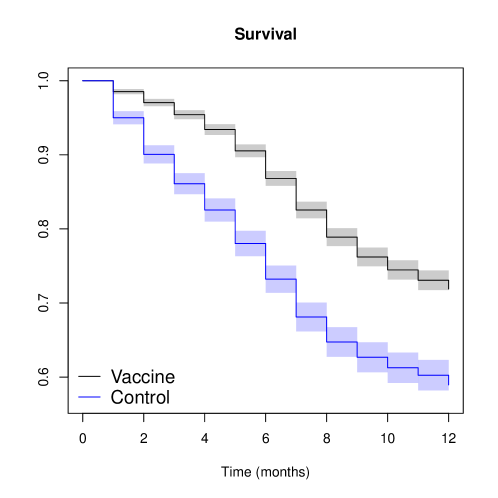
Figure 7. Kaplan-Meier survival estimates for the RTSS data by Benkeser et al. (2019). Confidence intervals are shown in shaded colors.

Investigators found that the instantaneous hazard of infection in the RTS,S/AS01 group increased over time relative to the hazard for recipients of the comparator vaccine, and concluded that

“[…] [S]tatistical models indicated nonproportionality of hazards over time. This could be due to waning vaccine efficacy, differential acquisition of natural immunity, or other factors that may influence the model, such as heterogeneity of exposure, the vaccine effect at the individual level, or both” (RTS,S Clinical Trials Partnership, 2012).

To investigate whether the vaccine protection waned over time, we computed the estimators described in Section 5 without any baseline covariates, reported in Table 5. Here, we let $k=1$ denote the interval from month 1 to the end of month 5 after baseline, and $k=2$ denote the interval from month 6 to the end of month 10.

Table 5. Estimates and 95% bootstrap confidence intervals for the synthetic RTSS dataset by Benkeser et al. (2019), computed using the estimators in Section 5 without baseline covariates. One-sided $95\%$ confidence intervals have been used for $\widehat{\mathcal{L}}_{2}(l)$, $\widehat{\mathcal{U}}_{2}(l)$, $\widehat{\mathcal{L}}_{\psi}(l)$ and $\widehat{\mathcal{U}}_{\psi}(l)$, whereas confidence intervals for $\widehat{\text{VE}}_{1}^{\mathrm{obs}},\widehat{\text{VE}}_{2}^{\mathrm{obs}}$ and $\widehat{\psi}^{\mathrm{obs}}(l)$ are two-sided.

Estimand	Estimate (95% CI)
$\widehat{\text{VE}}_{1}^{\text{obs}},\widehat{\text{VE}}_{1}^{\text{challenge}}$	$0.57(0.51,0.62)$
$\widehat{\text{VE}}_{2}^{\text{obs}}$	$0.17(0.07,0.26)$
$\widehat{\mathcal{L}}_{2}$	$-0.52(-0.69,-)$
$\widehat{\mathcal{U}}_{2}$	$0.59(-,0.61)$
$\widehat{\mathcal{L}}_{\psi}$	$0.28(0.24,-)$
$\widehat{\mathcal{U}}_{\psi}$	$1.04(-,1.16)$
$\widehat{\psi}^{\mathrm{obs}}$	$0.52(0.44,0.61)$

Additionally, we have computed the estimator $\widehat{\psi}^{\mathrm{obs}}=(1-\widehat{\text{VE}}_{1}^{\mathrm{obs}})/(1-\widehat{\text{VE}}_{2}^{\mathrm{obs}}$). Throughout this section, confidence intervals were computed using non-parametric bootstrap with 500 resamples.

The estimated bounds $\widehat{\mathcal{L}}_{\psi},\widehat{\mathcal{U}}_{\psi}$ contain the null-value 1, corresponding to no waning, and therefore do not rule out the possibility that the decline in $\text{VE}^{\mathrm{obs}}_{k}$ over time could be due to the depletion of susceptible individuals. However, $\widehat{\mathcal{U}}_{2}$ is close to $\text{VE}_{1}^{\mathrm{challenge}}$. A conditional analysis (Table 6 and Figure 8 (A)) using the baseline covariates age, sex and study site leads to the same conclusion: the point estimates of $\widehat{\mathcal{U}}_{\psi}(L)$ indicate waning ($\widehat{\mathcal{U}}_{\psi}(L)<1$) for a substantial proportion of the observed values of $L$ (Figure 8 (A)), but confidence intervals include the null value of no waning.

Table 6. Waning estimates and 95% bootstrap confidence intervals for the synthetic RTSS dataset by Benkeser et al. (2019), illustrated using 3 different combinations of baseline covariates

Age (weeks)	Sex	Study site	$\widehat{\text{VE}}_{1}^{\mathrm{obs}}(l)$	$\widehat{\text{VE}}_{2}^{\mathrm{obs}}(l)$	$\widehat{\mathcal{L}}_{2}(l)$	$\widehat{\mathcal{U}}_{2}(l)$	$\widehat{\mathcal{L}}_{\psi}(l)$	$\widehat{\mathcal{U}}_{\psi}(l)$	$\widehat{\psi}^{\mathrm{obs}}(l)$
51	female	1	0.74(0.62,0.81)	0.53(0.36,0.64)	0.30(0.10,-)	0.73(-,0.78)	0.38(0.33,-)	0.96(-,1.09)	0.56(0.46,0.68)
48	male	5	0.68(0.58,0.75)	0.44(0.27,0.57)	-0.01(-0.21,-)	0.66(-,0.72)	0.31(0.27,-)	0.94(-,1.07)	0.56(0.47,0.68)
58	male	3	0.55(0.43,0.64)	0.23(0.04,0.37)	-0.51(-0.72,-)	0.55(-,0.61)	0.30(0.25,-)	1.00(-,1.14)	0.58(0.50,0.69)

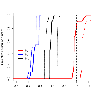
(a)

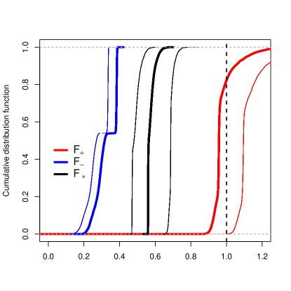
(b)

Figure 8. Cumulative distribution functions (cdf) of bounds and waning estimands. The blue curve is the empirical cdf $F_{-}$ of $\widehat{\mathcal{L}}_{\psi}(L)$, over the observed values of $L$. The black curve is the empirical cdf $F_{*}$ of $\widehat{\psi}^{\mathrm{obs}}(L)$, and the red curve is the empirical cdf $F_{+}$ of $\widehat{\mathcal{U}}_{\psi}(L)$. (A) Shows estimates with baseline covariates age, sex and study site (B) Shows estimates with baseline covariates age, weight for age (Z score), sex, study site, height for age (Z score), weight for height (Z score), arm circumference (Z score), hemoglobin, distance to nearest inpatient clinic, distance to nearest outpatient clinic and an indicator of rainy versus dry season. Point estimates are shown with thick lines, and 95% bootstrap confidence intervals with narrow lines.

As a sensitivity analysis, we repeated the analysis in Table 6 after breaking tied event times within each month by drawing random days, which gave nearly identical results. Furthermore, we performed a sensitivity analysis for the choice of baseline covariates, by including additional covariates in Figure 8 (B). The inclusion of additional covariates did not substantially change the distributions of estimates.

Appendix I Simulated example

In this section, we present simulations illustrating the use of logistic regression. Consider a hypothetical vaccine trial with individual-level data from months $k\in\{1,\dots K\}$ following vaccination, where we take $K=4$ (see e.g. Voysey et al. (2021)). Suppose the data were drawn from the following data generating mechanism. First sample $A,L$ according to

$$A \sim\mathrm{Ber}(1/2)\leavevmode\nobreak\ ,$$

$$L \sim\mathrm{Unif}[0,1]\leavevmode\nobreak\ .$$

Next, for $k\in\{1,\dots,K\}$, sample $C_{k}$ and $Y_{k}$ from the hazards

$$P(C_{k}=1\mid Y_{k-1}=0,C_{k-1}=0,A=a,L=l)=\beta_{C}\leavevmode\nobreak\ ,$$

(59) $$\Lambda_{k,a,l}=f_{k}(a,l;\beta_{k})=\operatorname*{expit}(\beta_{0,k}+\beta_{1,k}a+\beta_{2,k}l)\leavevmode\nobreak\ .$$

For each time interval $k$, we computed maximum likelihood estimates $\widehat{\beta}_{k}$ under the logistic model (59), and estimated $\mathcal{L}_{k}(l),\mathcal{U}_{k}(l)$ using (51). We computed confidence intervals using non-parametric bootstrap with $500$ resamples of $n=$ 10,000 individuals. The resulting estimates and confidence intervals are shown in Figure 9. In Figure 9 (A) and (B), the estimated bounds place informative constraints on the extent of vaccine waning, and are close in value to the observed vaccine efficacy $\text{VE}_{k}^{\mathrm{obs}}$. However, for the choice of parameters in Figure 9 (C) and (D), the bounds $\mathcal{L}_{k}(l),\mathcal{U}_{k}(l)$ differ substantially from $\text{VE}_{k}^{\mathrm{obs}}$, which illustrates that $\text{VE}_{k}^{\mathrm{challenge}}$ can be far greater (or smaller) than $\text{VE}_{k}^{\mathrm{obs}}$.

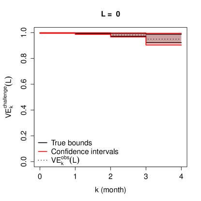
(a)

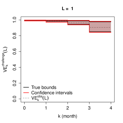
(b)

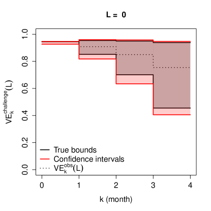
(c)

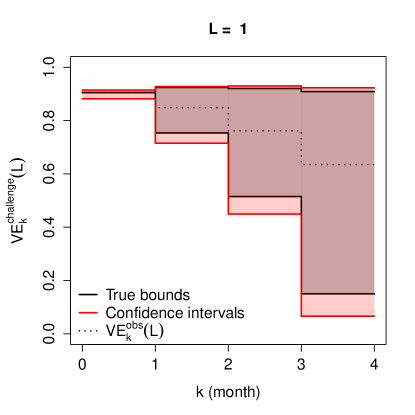
(d)

Figure 9. The true bounds $\mathcal{L}_{k},\mathcal{U}_{k}$ for baseline covariate levels $L=0$ and $L=1$ are shown together with one-sided 95% confidence intervals of $\widehat{\mathcal{L}}_{k},\widehat{\mathcal{U}}_{k}$, computed from non-parametric bootstrap with 500 resamples from a population of 10,000 individuals. (A) and (B) show a choice of parameters $(\beta_{C},\beta_{k})$ that gives narrow bounds, where $\text{VE}_{2}^{\mathrm{challenge}}$ is close to $\text{VE}_{2}^{\mathrm{obs}}$, while (C) and (D) show another choice of parameters that gives wider bounds.

Appendix J Further analyses

J.1. Sensitivity analysis of waning estimates

For $k\in\{1,2\}$, let $Q_{k}$ denote the exact time of the controlled exposure to a fixed quantity of the infectious agent during interval $k$, supposing that individuals are isolated from infectious exposures before and after this time. Suppose that Assumptions 1 (i) and (ii) for $e_{1}=0$, Assumptions 2-4 and Assumptions 7-12 hold. Let $q^{\dagger}$ denote the time that vaccine recipients are most protected against a controlled infectious exposure. We assume that this is after an immune response has developed a few days following the second dose of treatment, and before the immune response (potentially) begins to wane. Then, by definition,

$$E[\Delta Y_{1}^{a=1,q^{\dagger}}\mid L] \leq E[\Delta Y_{1}^{a=1,q}\mid L]\text{ w.p.\leavevmode\nobreak\ 1}\leavevmode\nobreak\ ,$$

for all $q$, which implies that

(60) $$E[\Delta Y_{1}^{a=1,q^{\dagger}}\mid L]\leq E_{G}[E_{G}[\Delta Y_{1}^{a=1,Q_{1}}\mid L]\mid E_{1}=1,A=1,L]\leavevmode\nobreak\ .$$

Furthermore, we will assume that Assumption 13 holds for any duration of time intervals, such that the timing of the controlled infectious exposure does not affect the risk of infectious outcomes in placebo recipients even within interval $k=1$. This implies that

(61) $$E[\Delta Y_{1}^{a=0,q=q^{\dagger}}\mid L]=E_{G}[E_{G}[\Delta Y_{1}^{a=0,Q_{1}}\mid L]\mid E_{1}=1,A=0,L]\leavevmode\nobreak\ .$$

Combining (60) and (61) with Proposition 2 gives

$$\frac{E[\Delta Y_{1}^{a=1,q^{\dagger}}\mid L]}{E[\Delta Y_{1}^{a=0,q^{\dagger}}\mid L]}\leq\frac{E[\Delta Y_{1}\mid A=1,L]}{E[\Delta Y_{1}\mid A=0,L]}\leavevmode\nobreak\ .$$

Thus, $\widehat{\text{VE}}_{1}^{\mathrm{obs}}$ is a conservative estimate of $\text{VE}_{1}^{\mathrm{challenge}}(l,q^{\dagger})$. Furthermore, under Assumption 13,

$$E[\Delta Y_{1}^{a=0,q^{\dagger}}\mid L]=E_{G}[E_{G}[\Delta Y_{2}^{a=0,q_{1}=0,Q_{2}^{q_{1}=0}}\mid L]\mid E_{2}^{q_{1}=0}=1,A=0,L]\leavevmode\nobreak\ .$$

Under the additional Assumptions 2-4, Proposition 2 gives

$$\frac{E[\Delta Y_{1}^{a=1,q^{\dagger}}\mid L]}{E_{G}[E_{G}[\Delta Y_{2}^{a=1,q_{1}=0,Q_{2}^{q_{1}=0}}\mid L]\mid E_{2}^{q_{1}=0}=1,A=1,L]}\leq\mathcal{U}_{\psi}\leavevmode\nobreak\ .$$

The left hand side is a contrast of a controlled infectious exposure at time $q^{\dagger}$ versus a randomly chosen time, $Q_{2}^{a,q_{1}=0}$, during interval $k=2$. Therefore, $\widehat{\mathcal{U}}_{\psi}$ conservatively estimates the extent of vaccine waning from interval 1 to 2.

In Tables 7-8, we perform a sensitivity analysis of the waning estimates reported in Table 1, using different choices of intervals $k=1$ and $k=2$.

Table 7. Estimates and 95% confidence intervals for (2), (5)-(6) and (12)-(13). Interval 1 ranged from 11 days after dose 1 until 2 months after dose 2 and interval 2 ranged from 2 months after dose 2 until the end of follow-up (chosen as day 190, see Table 2). Confidence intervals for the bounds $\mathcal{L}_{\bullet},\mathcal{U}_{\bullet}$ were one-sided, whereas two-sided confidence intervals were used for VE estimates.

Estimand	Estimate (95% CI)
$\widehat{\text{VE}}_{1}^{\text{obs}},\widehat{\text{VE}}_{1}^{\text{challenge}}$	$0.95(0.93,0.97)$
$\widehat{\text{VE}}_{2}^{\text{obs}}$	$0.88(0.84,0.90)$
$\widehat{\mathcal{L}}_{2}$	$0.86(0.83,-)$
$\widehat{\mathcal{U}}_{2}$	$0.91(-,0.93)$
$\widehat{\mathcal{L}}_{\psi}$	$0.33(0.23,-)$
$\widehat{\mathcal{U}}_{\psi}$	$0.54(-,0.84)$

Table 8. Illustrates two additional choices of interval $k=2$, denoted interval I and interval II. Interval I ranged from 7 days after dose 2 until 2 months after dose 2 and interval II ranged from 2 months after dose 2 until 4 months after dose 2. Interval $k=1$ ranged from dose 1 until the beginning of interval I (or II). Bootstrap confidence intervals (95%) for the bounds $\mathcal{L}_{\mathrm{I,II}},\mathcal{U}_{\mathrm{I,II}}$ are one-sided, whereas two-sided confidence intervals have been used for $\text{VE}^{\mathrm{obs}}_{\mathrm{I,II}}$. The naive contrast of $\text{VE}^{\mathrm{obs}}_{\mathrm{I}}$ vs. $\text{VE}^{\mathrm{obs}}_{\mathrm{II}}$ suggests that vaccine protection waned, but the bounds $[\mathcal{L}^{\mathrm{obs}}_{\mathrm{I}},\mathcal{U}^{\mathrm{obs}}_{\mathrm{I}}]$ and $[\mathcal{L}^{\mathrm{obs}}_{\mathrm{II}},\mathcal{U}^{\mathrm{obs}}_{\mathrm{II}}]$ overlap and are wide due to the substantial number of depleted individuals from dose 1 until the beginning of intervals I and II.

Estimand	Estimate (95% CI)
$\widehat{\text{VE}}_{\mathrm{I}}^{\text{obs}}$	$0.96(0.93,0.98)$
$\widehat{\mathcal{L}}_{\mathrm{I}}$	$0.83(0.79,-)$
$\widehat{\mathcal{U}}_{\mathrm{I}}$	$0.97(-,0.98)$
$\widehat{\text{VE}}_{\mathrm{II}}^{\text{obs}}$	$0.90(0.87,0.93)$
$\widehat{\mathcal{L}}_{\mathrm{II}}$	$0.81(0.77,-)$
$\widehat{\mathcal{U}}_{\mathrm{II}}$	$0.94(-,0.96)$

In the bounds (50), we identified $E[Y_{k}^{\overline{c}=0}\mid A=a,L]$ by $\sum_{k^{\prime}=1}^{k}\Lambda_{k^{\prime},a,L}$ under Assumption 24. The leading order correction is of order $(\sum_{k^{\prime}=1}^{k}\Lambda_{k^{\prime},a,L})^{2}$, seen by Taylor expanding the approximation $E[\Delta Y_{k}^{\overline{c}=0}\mid A=a,L]\approx 1-\exp(\sum_{k^{\prime}=1}^{k}\Lambda_{k^{\prime},a,L})$, which is small since the cumulative hazard point estimates during intervals 1 and 2 (for the choice of intervals in Table 1) were given by $\widehat{\Lambda}_{k=1,a=0}=0.020$, $\widehat{\Lambda}_{k=1,a=1}=0.001$, $\widehat{\Lambda}_{k=2,a=0}=0.029$ and $\widehat{\Lambda}_{k=2,a=1}=0.003$.

J.2. Comparison against reported confidence intervals

By computing confidence intervals (57) of $\text{VE}_{k,j}^{\mathrm{obs}}$ (Table 9), we illustrate that our approach gives identical point estimates and nearly identical confidence intervals to Thomas et al. (2021).

Table 9. Validation of point estimates and confidence intervals computed from (57), against corresponding numbers reported in Figure 2 of Thomas et al. (2021)

	Confidence interval (computed from (57))	Confidence interval (Thomas et al. (2021))
Overall	$0.878(0.853,0.898)$	$0.878(0.853,0.899)$
After dose 1 up to dose 2	$0.584(0.414,0.705)$	$0.584(0.408,0.712)$
$<11$ days after dose 1	$0.182(-0.236,0.459)$	$0.182(-0.261,0.473)$
$\geq 11$ days after dose 1 until dose 2	$0.917(0.794,0.967)$	$0.917(0.796,0.974)$
After dose 2 until $<7$ days after	$0.915(0.723,0.974)$	$0.915(0.729,0.983)$
$\geq 7$ days after dose 2	$0.912(0.889,0.930)$	$0.912(0.889,0.930)$
$\geq 7$ days after dose 2 until $<2$ months after	$0.962(0.932,0.979)$	$0.962(0.933,0.981)$
$\geq 2$ months after dose 2 until $<4$ months after dose 2	$0.901(0.867,0.927)$	$0.901(0.866,0.929)$
$\geq 4$ months after dose 2	$0.837(0.748,0.895)$	$0.837(0.747,0.899)$

J.3. Subgroup analysis

Let $\widehat{\lambda}_{a,l}=N_{a,l}/T_{a,l}$, where $N_{a,l}$ and $T_{a,l}$ are the overall number of recorded events and person time at risk for treatment group $A=a$ and baseline covariates $L=l$. The confidence interval

(62) $$CI(\widehat{\lambda}_{a,l})=\widehat{\lambda}_{a,l}\exp\left(\pm\frac{z_{1-\alpha/2}}{\sqrt{N_{a,l}}}\right)$$

is asymptotically valid in large samples under Assumption 24 by Theorem 8.22 in Lehmann and Casella (1998) with transformation $h(\lambda_{a,l})=\log\lambda_{a,l}$. Assuming a constant hazard $\lambda_{a,l}$ during time $[0,\tau]$, the survival by day $\tau$ is given by $\exp(-\lambda_{a,l}\tau)$ and conversely the cumulative incidence by $\mu_{a,l}=1-\exp(-\lambda_{a,l}\tau)$. Then, using a log-minus-log transformation of the survival (Aalen et al., 2008) together with (62) gives the confidence interval

(63) $$CI(\widehat{\mu}_{a,l})=1-\exp\left\{-\widehat{\lambda}_{a,l}\tau\exp\left(\pm\frac{z_{1-\alpha/2}}{\sqrt{N_{a,l}}}\right)\right\}\leavevmode\nobreak\ .$$

Confidence intervals for conditional hazards and cumulative incidences overlap for the different subgroups $L$ (Table 10).

Table 10. Hazard point estimates and 95% confidence intervals (62)-(63) by subgroup $A=a,L=l$, computed using Table S7 in the Supplementary Appendix of Thomas et al. (2021). Hazards are given in units of $10^{-5}\textrm{days}^{-1}$. Cumulative incidences are evaluated on day $\tau=190$.

	$CI(\widehat{\lambda}_{a=1,l})$	$CI(\widehat{\lambda}_{a=0,l})$	$CI(\widehat{\mu}_{a=1,l})$	$CI(\widehat{\mu}_{a=0,l})$
Overall	$3.38(2.70,4.22)$	$38.79(36.27,41.49)$	$0.006(0.005,0.008)$	$0.071(0.067,0.076)$
At risk: Yes	$3.43(2.46,4.77)$	$40.98(37.16,45.19)$	$0.006(0.005,0.009)$	$0.075(0.068,0.082)$
At risk: No	$3.34(2.46,4.51)$	$37.03(33.76,40.62)$	$0.006(0.005,0.009)$	$0.068(0.062,0.074)$
Age 16-64 and at risk	$3.81(2.65,5.49)$	$44.68(40.07,49.81)$	$0.007(0.005,0.010)$	$0.081(0.073,0.090)$
Age 65 or older and at risk	$2.42(1.09,5.38)$	$29.65(23.50,37.42)$	$0.005(0.002,0.010)$	$0.055(0.044,0.069)$
Obese: Yes	$3.52(2.41,5.13)$	$41.96(37.57,46.87)$	$0.007(0.005,0.010)$	$0.077(0.069,0.085)$
Obese: No	$3.31(2.51,4.36)$	$37.16(34.14,40.44)$	$0.006(0.005,0.008)$	$0.068(0.063,0.074)$
Age 16-64 and obese	$3.91(2.62,5.84)$	$44.87(39.79,50.60)$	$0.007(0.005,0.011)$	$0.082(0.073,0.092)$
Age 65 or older and obese	$2.03(0.66,6.31)$	$30.07(22.45,40.27)$	$0.004(0.001,0.012)$	$0.056(0.042,0.074)$

J.4. Challenge estimands that use antibody titers

In this section, we show how the challenge effect can be used to quantify the relation between immunological markers and vaccine waning. Let

$$\psi(l_{0},l_{1})=\frac{E[\Delta Y_{2}^{a=1,e_{1}=0,e_{2}=1}\mid L_{1}^{a=1}=l_{1},L_{0}=l_{0}]}{E[\Delta Y_{1}^{a=1,e_{1}=1}\mid L_{1}^{a=1}=l_{1},L_{0}=l_{0}]}\leavevmode\nobreak\ ,$$

where $L_{1}^{a=1}$ is an immunological marker, e.g. antibody titer, measured at the beginning of interval 1 under an intervention that assigns vaccine $a$ and $L_{0}$ is a vector of baseline covariates. The estimand corresponds to the answer of the following plain-English question: to what extent does the amount of waning depend on the initial antibody response? If $\psi(l_{0},l_{1})$ is small for $l_{1}=l_{-}$, but large for $l_{1}=l_{+}$, then we might justify that individuals with $l_{1}=l_{-}$ are prioritized to receive booster vaccination before individuals with $l_{1}=l_{+}$.

Let $L_{2}$ denote a measurement of antibody titer at the beginning of time interval 2. Then,

$$\phi(l_{0},l_{1},l_{2})=\frac{E[\Delta Y_{2}^{a=1,e_{1}=0,e_{2}=1}\mid L_{2}^{a=1,e_{1}=0}=l_{2},L_{1}^{a=1}=l_{1},L_{0}=l_{0}]}{E[\Delta Y_{2}^{a=1,e_{1}=0,e_{2}=1}\mid L_{0}=l_{0}]}$$

is the relative risk of outcomes under the antibody profile $(l_{1},l_{2})$. Unlike the naive contrast

$$\phi^{\mathrm{obs}}(l_{0},l_{1},l_{2})=\frac{E[\Delta Y_{2}\mid\Delta Y_{1}=0,L_{2}=l_{2},L_{1}=l_{1},L_{0}=l_{0},A=1]}{E[\Delta Y_{2}\mid\Delta Y_{1}=0,L_{0}=l_{0},A=1]}\leavevmode\nobreak\ ,$$

the conditional challenge effect $\phi(l_{0},l_{1},l_{2})$ is not subject to depletion of susceptible individuals during interval 1. If $\phi(l_{0},l_{1},l_{2})>1$ then individuals with $(L_{1}=l_{1},L_{2}=l_{2})$ are less protected during interval 2, and should be prioritized for a booster dose among those who initially received the vaccine. This estimand describes heterogeneity in vaccine protection across antibody responses.

Identification results for $\psi(l_{0},l_{1})$ and $\phi(l_{0},l_{1},l_{2})$ can be derived similarly to Theorem 1 and Proposition 1, but require some additional assumptions, which also are single world; they are in-principle testable in future challenge experiments (Richardson and Robins, 2013). These estimands will be studied thoroughly in future research.

Finally, antibody measurements can also be used for sensitivity analyses. For example, one could compare the distribution of antibodies in event-free individuals by time $k$ ($\Delta Y_{k}=0$), for different values of $k$ as a measure of the depletion of susceptible individuals.

References

• Aalen et al. (2008) Odd O. Aalen, Ørnulf Borgan, and Håkon K. Gjessing. Survival and Event History Analysis. Statistics for Biology and Health. Springer New York, New York, NY, 2008.
• Bardsley et al. (2023) Megan Bardsley, Roger A. Morbey, Helen E. Hughes, Charles R. Beck, Conall H. Watson, Hongxin Zhao, Joanna Ellis, Gillian E. Smith, and Alex J. Elliot. Epidemiology of respiratory syncytial virus in children younger than 5 years in England during the COVID-19 pandemic, measured by laboratory, clinical, and syndromic surveillance: a retrospective observational study. The Lancet Infectious Diseases, 23(1):56–66, 2023.
• Benkeser et al. (2019) David Benkeser, Peter B. Gilbert, and Marco Carone. Estimating and Testing Vaccine Sieve Effects Using Machine Learning. Journal of the American Statistical Association, 114(527):1038–1049, 2019.
• Bergwerk et al. (2021) Moriah Bergwerk et al. Covid-19 Breakthrough Infections in Vaccinated Health Care Workers. New England Journal of Medicine, 385(16):1474–1484, 2021.
• Bie et al. (1987) Ole Bie, Ørnulf Borgan, and Knut Liestøl. Confidence Intervals and Confidence Bands for the Cumulative Hazard Rate Function and Their Small Sample Properties. Scandinavian Journal of Statistics, 14(3):221–233, 1987.
• Cox (1972) D. R. Cox. Regression Models and Life-Tables. Journal of the Royal Statistical Society: Series B (Methodological), 34(2):187–202, 1972.
• Cox (1958) David Roxbee Cox. Planning of experiments. Wiley series in probability and mathematical statistics. Applied probability and statistics. J. Wiley, New York, 1958.
• DeHaan et al. (2022) Elliot DeHaan, Joseph P. McGowan, Steven M. Fine, Rona Vail, Samuel T. Merrick, Asa Radix, Christopher J. Hoffmann, and Charles J. Gonzalez. PEP to Prevent HIV Infection. New York State Department of Health AIDS Institute Clinical Guidelines. Johns Hopkins University, Baltimore (MD), 2022.
• Ewell (1996) Marian Ewell. Comparing Methods for Calculating Confidence Intervals for Vaccine Efficacy. Statistics in Medicine, 15(21):2379–2392, 1996.
• Fintzi and Follmann (2021) Jonathan Fintzi and Dean Follmann. Assessing Vaccine Durability in Randomized Trials Following Placebo Crossover. arXiv preprint arXiv:2101.01295 [stat], 2021.
• Follmann et al. (2022) Dean Follmann, Michael Fay, and Craig Magaret. Estimation of vaccine efficacy for variants that emerge after the placebo group is vaccinated. Statistics in Medicine, 41(16):3076–3089, 2022.
• Follmann et al. (2020) Dean Follmann et al. Assessing Durability of Vaccine Effect Following Blinded Crossover in COVID-19 Vaccine Efficacy Trials. medRxiv, 2020.
• Follmann et al. (2021) Dean Follmann et al. A Deferred-Vaccination Design to Assess Durability of COVID-19 Vaccine Effect After the Placebo Group Is Vaccinated. Annals of Internal Medicine, 174(8):1118–1125, 2021.
• Goldberg et al. (2021) Yair Goldberg, Micha Mandel, Yinon M. Bar-On, Omri Bodenheimer, Laurence Freedman, Eric J. Haas, Ron Milo, Sharon Alroy-Preis, Nachman Ash, and Amit Huppert. Waning Immunity after the BNT162b2 Vaccine in Israel. New England Journal of Medicine, 385(24):e85, 2021.
• Halloran and Struchiner (1995) M. Elizabeth Halloran and Claudio J. Struchiner. Causal Inference in Infectious Diseases. Epidemiology, 6(2):142–151, 1995.
• Halloran et al. (1992) M. Elizabeth Halloran, Michael Haber, and Ira M. Longini, Jr. Interpretation and Estimation of Vaccine Efficacy under Heterogeneity. American Journal of Epidemiology, 136(3):328–343, 1992.
• Halloran et al. (1996) M. Elizabeth Halloran, Ira M. Longini, Jr., and Claudio J. Struchiner. Estimability and Interpretation of Vaccine Efficacy Using Frailty Mixing Models. American Journal of Epidemiology, 144(1):83–97, 1996.
• Halloran et al. (1997) M. Elizabeth Halloran, Claudio J. Struchiner, and Ira M. Longini, Jr. Study Designs for Evaluating Different Efficacy and Effectiveness Aspects of Vaccines. American Journal of Epidemiology, 146(10):789–803, 1997.
• Halloran et al. (1999) M. Elizabeth Halloran, Ira M. Longini, Jr., and Claudio J. Struchiner. Design and interpretation of vaccine field studies. Epidemiologic Reviews, 21(1):73–88, 1999.
• Halloran et al. (2012) M. Elizabeth Halloran, Ira M. Longini, Jr., and Claudio J. Struchiner. Design and Analysis of Vaccine Studies. Springer, 2010th edition edition, 2012.
• Hausman (2021) Daniel M. Hausman. Challenge Trials: What Are the Ethical Problems? The Journal of Medicine and Philosophy: A Forum for Bioethics and Philosophy of Medicine, 46(1):137–145, 2021.
• Hernán (2016) Miguel A. Hernán. Does water kill? A call for less casual causal inferences. Annals of Epidemiology, 26(10):674–680, 2016.
• Hernán and Monge (2023) Miguel A. Hernán and Susana Monge. Selection bias due to conditioning on a collider. BMJ, 381:p1135, 2023.
• Hernán and Robins (2020) Miguel A. Hernán and James M. Robins. Causal Inference: What If. Boca Raton: Chapman & Hall/CRC, 2020.
• Hernán et al. (2022) Miguel A. Hernán, Wei Wang, and David E. Leaf. Target Trial Emulation: A Framework for Causal Inference From Observational Data. JAMA, 328(24):2446–2447, 2022.
• Horowitz and Manski (2000) Joel L. Horowitz and Charles F. Manski. Nonparametric Analysis of Randomized Experiments with Missing Covariate and Outcome Data. Journal of the American Statistical Association, 95(449):77–84, 2000.
• Hudgens et al. (2004) Michael G. Hudgens, Peter B. Gilbert, and Steven G. Self. Endpoints in vaccine trials. Statistical Methods in Medical Research, 13(2):89–114, 2004.
• Huitfeldt et al. (2019) Anders Huitfeldt, Mats J. Stensrud, and Etsuji Suzuki. On the collapsibility of measures of effect in the counterfactual causal framework. Emerging Themes in Epidemiology, 16(1):1, 2019.
• Janvin et al. (2023) Matias Janvin, Jessica G. Young, Pål C. Ryalen, and Mats J. Stensrud. Causal inference with recurrent and competing events. Lifetime Data Analysis, 2023.
• Kanaan and Farrington (2002) Mona N. Kanaan and C. Paddy Farrington. Estimation of Waning Vaccine Efficacy. Journal of the American Statistical Association, 97(458):389–397, 2002.
• Khoury et al. (2021) David S. Khoury et al. Neutralizing antibody levels are highly predictive of immune protection from symptomatic SARS-CoV-2 infection. Nature Medicine, 27(7):1205–1211, 2021.
• Killingley et al. (2022) Ben Killingley et al. Safety, tolerability and viral kinetics during SARS-CoV-2 human challenge in young adults. Nature Medicine, 28(5):1031–1041, 2022.
• Lehmann and Casella (1998) Erich L. Lehmann and George Casella. Theory of point estimation. Springer texts in statistics. Springer, New York, 2nd ed edition, 1998.
• Levin et al. (2021) Einav G. Levin et al. Waning Immune Humoral Response to BNT162b2 Covid-19 Vaccine over 6 Months. New England Journal of Medicine, 385(24):e84, 2021.
• Lin et al. (2021) Dan-Yu Lin, Donglin Zeng, and Peter B. Gilbert. Evaluating the Long-term Efficacy of Coronavirus Disease 2019 (COVID-19) Vaccines. Clinical Infectious Diseases, 73(10):1927–1939, 2021.
• Lipsitch et al. (2019) M. Lipsitch, E. Goldstein, G. T. Ray, and B. Fireman. Depletion-of-susceptibles bias in influenza vaccine waning studies: how to ensure robust results. Epidemiology & Infection, 147:e306, 2019.
• Mathieu et al. (2020) Edouard Mathieu, Hannah Ritchie, Lucas Rodés-Guirao, Cameron Appel, Charlie Giattino, Joe Hasell, Bobbie Macdonald, Saloni Dattani, Diana Beltekian, Esteban Ortiz-Ospina, and Max Roser. Coronavirus Pandemic (COVID-19). Our World in Data, 2020.
• Meyerowitz et al. (2021) Eric A. Meyerowitz, Aaron Richterman, Rajesh T. Gandhi, and Paul E. Sax. Transmission of SARS-CoV-2: A Review of Viral, Host, and Environmental Factors. Annals of Internal Medicine, 174(1):69–79, 2021.
• Mischlinger et al. (2020) Johannes Mischlinger, Caroline Rönnberg, Míriam J. Álvarez Martínez, Silja Bühler, Małgorzata Paul, Patricia Schlagenhauf, Eskild Petersen, and Michael Ramharter. Imported Malaria in Countries where Malaria Is Not Endemic: a Comparison of Semi-immune and Nonimmune Travelers. Clinical Microbiology Reviews, 33(2):10.1128/cmr.00104–19, 2020.
• Monge et al. (2023) Susana Monge, Roberto Pastor-Barriuso, and Miguel A Hernán. The imprinting effect of covid-19 vaccines: an expected selection bias in observational studies. BMJ, 381, 2023.
• Pearl (2009) Judea Pearl. Causality: models, reasoning, and inference. Cambridge University Press, Cambridge, 2nd edition, 2009.
• Pearl (2010) Judea Pearl. On the Consistency Rule in Causal Inference: Axiom, Definition, Assumption, or Theorem? Epidemiology, 21(6):872, 2010.
• Polack et al. (2020) Fernando P. Polack et al. Safety and Efficacy of the BNT162b2 mRNA Covid-19 Vaccine. New England Journal of Medicine, 383(27):2603–2615, 2020.
• Ray et al. (2019) G Thomas Ray, Ned Lewis, Nicola P Klein, Matthew F Daley, Shirley V Wang, Martin Kulldorff, and Bruce Fireman. Intraseason Waning of Influenza Vaccine Effectiveness. Clinical Infectious Diseases, 68(10):1623–1630, 2019.
• Ray et al. (2020) G. Thomas Ray, Ned Lewis, Nicola P. Klein, Matthew F. Daley, Marc Lipsitch, and Bruce Fireman. Depletion-of-susceptibles Bias in Analyses of Intra-season Waning of Influenza Vaccine Effectiveness. Clinical Infectious Diseases, 70(7):1484–1486, 2020.
• Richardson and Robins (2013) Thomas S. Richardson and James M. Robins. Single World Intervention Graphs (SWIGs): A Unification of the Counterfactual and Graphical Approaches to Causality. 2013.
• Robins (1986) James M. Robins. A new approach to causal inference in mortality studies with a sustained exposure period—application to control of the healthy worker survivor effect. Mathematical Modelling, 7(9):1393–1512, 1986.
• Robins and Richardson (2011) James M. Robins and Thomas S. Richardson. Alternative Graphical Causal Models and the Identification of Direct Effects. In Causality and Psychopathology. Oxford University Press, 2011.
• Robins et al. (2021) James M. Robins, Thomas S. Richardson, and Ilya Shpitser. An Interventionist Approach to Mediation Analysis. arXiv:2008.06019 [stat], 2021.
• Roestenberg et al. (2012) Meta Roestenberg, Sake J. de Vlas, An-Emmie Nieman, Robert W. Sauerwein, and Cornelus C. Hermsen. Efficacy of Preerythrocytic and Blood-Stage Malaria Vaccines Can Be Assessed in Small Sporozoite Challenge Trials in Human Volunteers. The Journal of Infectious Diseases, 206(3):319–323, 2012.
• RTS,S Clinical Trials Partnership (2011) RTS,S Clinical Trials Partnership. First Results of Phase 3 Trial of RTS,S/AS01 Malaria Vaccine in African Children. New England Journal of Medicine, 365(20):1863–1875, 2011.
• RTS,S Clinical Trials Partnership (2012) RTS,S Clinical Trials Partnership. A Phase 3 Trial of RTS,S/AS01 Malaria Vaccine in African Infants. New England Journal of Medicine, 367(24):2284–2295, 2012.
• Rubin et al. (2022) Eric J. Rubin, Lindsey R. Baden, and Stephen Morrissey. Audio Interview: Waning Immunity against Covid-19. New England Journal of Medicine, 386(21):e64, 2022.
• Smith et al. (1984) Peter G. Smith, Laura C. Rodrigues, and Paul E. M. Fine. Assessment of the Protective Efficacy of Vaccines against Common Diseases Using Case-Control and Cohort Studies. International Journal of Epidemiology, 13(1):87–93, 1984.
• Stensrud and Smith (2023) Mats J. Stensrud and Louisa Smith. Identification of Vaccine Effects When Exposure Status Is Unknown. Epidemiology, 34(2):216–224, 2023.
• Struchiner and Halloran (2007) C. J. Struchiner and M. E. Halloran. Randomization and baseline transmission in vaccine field trials. Epidemiology and Infection, 135(2):181–194, 2007.
• Therneau (2023) Terry Therneau. A package for survival analysis in R. R package version 3.5-7. 2023.
• Therneau and Grambsch (2000) Terry M. Therneau and Patricia M. Grambsch. Modeling Survival Data: Extending the Cox Model. Statistics for Biology and Health. Springer New York, New York, NY, 2000.
• Thomas et al. (2021) Stephen J. Thomas et al. Safety and Efficacy of the BNT162b2 mRNA Covid-19 Vaccine through 6 Months. New England Journal of Medicine, 385(19):1761–1773, 2021.
• Tsiatis and Davidian (2022) Anastasios A. Tsiatis and Marie Davidian. Estimating vaccine efficacy over time after a randomized study is unblinded. Biometrics, 78(3):825–838, 2022.
• United States Census Bureau (2024) United States Census Bureau. Population Clock, 2024.
• VanderWeele (2022) Tyler J. VanderWeele. Constructed Measures and Causal Inference. Epidemiology (Cambridge, Mass.), 33(1):141–151, 2022.
• VanderWeele and Hernán (2013) Tyler J. VanderWeele and Miguel A. Hernán. Causal Inference Under Multiple Versions of Treatment. Journal of causal inference, 1(1):1–20, 2013.
• Voysey et al. (2021) Merryn Voysey et al. Safety and efficacy of the ChAdOx1 nCoV-19 vaccine (AZD1222) against SARS-CoV-2: an interim analysis of four randomised controlled trials in Brazil, South Africa, and the UK. The Lancet, 397(10269):99–111, 2021.
• Wei et al. (2022) Qinyu Wei, Peng Wang, and Ping Yin. Confidence interval estimation for vaccine efficacy against covid-19. Frontiers in Public Health, 10, 2022.