On Nanowire Morphological Instability and Pinch-Off by Surface Electromigration

Abstract

Surface diffusion and surface electromigration may lead to a morphological instability of thin solid films and nanowires. In this paper two nonlinear analyzes of a morphological instability are developed for a single-crystal cylindrical nanowire that is subjected to the axial current. These treatments extend the conventional linear stability analyzes without surface electromigration, that manifest a Rayleigh-Plateau instability. A weakly nonlinear analysis is done slightly above the Rayleigh-Plateau (longwave) instability threshold. It results in a one-dimensional Sivashinsky amplitude equation that describes a blow-up of a surface perturbation amplitude in a finite time. This is a signature of a formation of an axisymmetric spike singularity of a cylinder radius, which leads to a wire pinch-off and separation into a disjoint segments. The scaling analysis of the amplitude spike singularity is performed, and the time-and-electric field-dependent dimensions of the spike are characterized. A weakly nonlinear multi-scale analysis is done at the arbitrary distance above a longwave or a shortwave instability threshold. The time-and-electric field-dependent Fourier amplitudes of the major instability modes are derived and characterized.

Keywords:  Nanowires, morphological stability, electromigration, singular solutions of PDEs, weakly nonlinear analysis, scaling analysis, multi-scale analysis

I Introduction

Surface electromigration [1, 2, 3] is a well-known and efficient method to guide morphological changes of thin films by surface diffusion. In particular, it has been used to manufacture nanocontacts by breaking of thin films and nanowires via a controlled pinch-offs [4, 5, 6]. Such nanocontacts are required for engineering and biomedical applications, for example, for measurement of the electrical conductance and electronic properties of a molecule, but forming a quality nanocontact is still a major challenge [7]. To overcome that challenge, the first step should be a basic understanding of a surface electromigration-driven morphological instability of a single-crystal wire that leads to a pinch-off event.

Modeling morphological instabilities of nanowires by a classical approach of accounting for surface diffusion via an evolution partial differential equation (PDE) for a shape variable [8, 9, 10] flourished in the 1990s and early 2000s [11, 12, 13, 14, 15, 16, 17]. A recent paper emphasizing this approach is by Wang et al. [18]. These authors considered a surface area minimization problem, computed a wire pinch-off using a phase-field method, and extended the Rayleigh-Plateau stability condition to finite amplitude perturbations. Also a limited Monte Carlo computations were published [19]. For predictive applied modeling of a nanocontact fabrication process a multi-physics framework is needed, that explicitly includes a model and a computation of a nanowire pinch-off instability, whereby the latter is triggered and enhanced by the surface current. Since the cited works do not consider the key mass transport mechanism, namely surface electromigration (shortened to electromigration in the rest of the paper), they cannot form a basis for that framework.

Toward the stated goal, in Ref. [20] this author introduced a PDE-based model for electromigrated cylindrical nanowire deposited on a substrate. That model is complicated by the presence of the contact lines and a non-axisymmetric surface instability modes. A linear stability analysis (LSA) of that model is performed in Ref. [20], from which a simpler case of axisymmetrically evolving free-standing wire is easily recovered. Axisymmetric modes dominate evolution of surface perturbations for a free-standing wire in the absence of electromigration, i.e. when only a natural high-temperature surface diffusion is operative [11]. Provided the axial current and a corresponding diffusion anisotropy that is a function of the axial variable, this is expected to hold when the electromigration is also operative. Ref. [21] reports a computation of a wire breakup into a chain set of particles for the simpler case. The breakup time and the number of particles that emerge upon a breakup are characterized as a function of the initial surface roughness.

In this communication, also for the axisymmetrically evolving free-standing wire, in Sec. III we perform a weakly nonlinear analysis slightly above the longwave instability threshold. This analysis assumes, as follows from LSA, that a critical (the most dangerous, i.e. the fastest growing) surface sinusoidal perturbation has a tiny wavenumber $k\rightarrow 0$. According to weakly nonlinear theory, such perturbation would develop into a protruding axisymmetric spikes from the surface toward the wire axis, the spikes being spaced along the wire axis with the separation distance $2\pi/k$, i.e. the spikes form via the deepening and sharpening of the minima of a critical perturbation. This is a weakly nonlinear scenario of a wire pinch-off and its breakup into a set of nanoparticles. From this analysis we obtain a much needed information on the time-and-electric field-dependent dimensions of the spike when the spike is not too deep, i.e. when the surface deviation from the cylindricity is not too large, so that a nonlinearity is weak. Mathematically, the latter is equivalent to a derivation of an amplitude equation via the expansion of a governing PDE up to the terms that are quadratic in the perturbation amplitude (whereas LSA is based on the expansion up to linear terms, i.e. a linearization procedure, which assumes that a perturbation amplitude is tiny). In other words, a perturbation amplitude is finite in the weakly nonlinear analysis. This key underlying assumption is the same in this paper and in Ref. [18]. A finite amplitude is quite likely to occur in the experiment [22].

Independent of weakly nonlinear analysis, in Sec. IV we start with the assumption of the initial unstable surface perturbation having an arbitrary finite wavenumber $0<k<k_{c}$, where $k_{c}$ is the instability cut-off wavenumber from LSA, and ask which unstable surface modes are the fastest growing. In this weakly nonlinear multi-scale treatment the spike formation is not considered. (As in the “standard” weakly nonlinear analysis in Sec. III, the governing PDE for the surface variable will be expanded to second order in a small parameter that has a meaning of a perturbation amplitude. This explains why we use the term “weakly nonlinear multi-scale analysis”.) Nonlinearity of the governing PDE forces a fast distortion of the initial sinusoidal surface perturbation into a general smooth surface shape, and as was just explained, we are interested in finding the fastest growing Fourier modes in its spectrum.

II The model

We consider surface electromigration on a free-standing cylindrical nanowire of radius $R_{0}$. (For details of the model derivation, see Ref. [20].) Assuming axial symmetry and a constant electric field $E_{0}$ in the axial direction, the wire radius $r(t,y)$ is governed by a nonlinear dimensionless evolution PDE:

$$r_{t}=\frac{1}{r}\frac{\partial}{\partial y}\left[M(r_{y})\frac{rK_{y}+E}{\sqrt{1+r_{y}^{2}}}\right],$$ (1)

where $y$ is the axial variable,

$$K=\frac{1}{r\sqrt{1+r_{y}^{2}}}-\frac{r_{yy}}{\left(1+r_{y}^{2}\right)^{3/2}}$$ (2)

the mean curvature of the surface, and

$$M(r_{y})=\frac{1+S\cos^{2}{\left(\arctan{r_{y}}+\psi\right)}}{1+S}$$ (3)

the anisotropic diffusional mobility of the adsorbed atoms (adatoms) [23]. Here $S>0$ is the anisotropy strength and $0\leq\psi\leq\pi/2$ the misorientation angle for a wire oriented along [100] crystallographic direction. Also $E=Q\Delta VR_{0}^{2}/(\Omega\gamma\ell)$ is the electric field parameter, where $Q>0$ is the effective charge of ionized adatoms, $\Delta V$ a voltage difference between the front and back faces of a wire, $\ell$ the wire length, $\Omega$ the atomic volume, and $\gamma$ the surface energy. Note that $E_{0}=\Delta V/\ell$, and thus a positivity (a negativity) of $E_{0}$ and $E$ depends on the sign of $\Delta V$. When surface diffusion is isotropic ($S=0\rightarrow M(r_{y})=1$) and the electric field is off ($E=0$), Eq. (1) reduces to a well-known evolution equation $r_{t}=\frac{1}{r}\frac{\partial}{\partial y}\left[\frac{rK_{y}}{\left(1+r_{y}^{2}\right)^{1/2}}\right]$ [11, 12], which expresses only the adatom surface diffusion via a surface Laplacian of mean curvature.

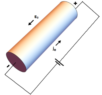
Figure 1: Unperturbed cylindrical nanowire (the base state). $j_{e}$ is the surface electric current that drives the surface electromigration of adatoms via the ”electron wind” [1, 2, 3].

II.1 LSA

Eq. (1) has the trivial solution $r=1$ (the base state), corresponding to unperturbed cylinder. Introducing a tiny perturbation of the base state, $r=1+\xi_{0}e^{\sigma t}\cos{ky},\;\xi_{0}\ll 1$, and linearizing in $\xi_{0}$ gives the growth rate $\sigma$ and the instability cut-off wavenumber $k_{c}$ [20]:

$$\sigma(k;E)=\frac{2+S(1+\cos{2\psi})}{2(1+S)}k^{2}\left(1-k^{2}\right)+E\frac{S\sin{2\psi}}{1+S}k^{2}\equiv\frac{\alpha_{1}+\alpha_{3}}{2\left(\alpha_{3}-1\right)}k^{2}\left(1-k^{2}\right)+\frac{\alpha_{2}}{\alpha_{3}-1}Ek^{2},$$ (4)

$$k_{c}(E)=\sqrt{1+\frac{2SE\sin{2\psi}}{2+S(1+\cos{2\psi})}}\equiv\sqrt{1+\frac{2\alpha_{2}E}{\alpha_{1}+\alpha_{3}}}.$$ (5)

Perturbations with a wavenumbers $0<k<k_{c}(E)$ destabilize the base state, since for these wavenumbers $\sigma(k;E)>0$. This is a longwave instability. Here we introduced a non-negative parameters $\alpha_{1}=S\cos{2\psi},\alpha_{2}=S\sin{2\psi}$ and a positive parameter $\alpha_{3}=2+S$. At $S=0$ (isotropy) with either $E=0$, or $E\neq 0$, Eqs. (4) and (5) reduce to $\sigma(k;0)=k^{2}(1-k^{2})$ and $k_{c}(0)=1$, respectively, which characterize a classical Rayleigh-Plateau instability of a free-standing solid wire [8]. In dimensional coordinates this implies that an axisymmetric sinusoidal perturbation induces instability if and only if its wavelength is longer than the circumference of the undisturbed cylinder.

Setting $\sigma=0$ results in the neutral stability curve $E(k)=\frac{\alpha_{1}+\alpha_{3}}{2\alpha_{2}}\left(k^{2}-1\right)$. Fig. 2 shows this curve for $S=1$ and $\psi=\pi/12$ [20] (these values are fixed for the remainder of this paper).

Figure 2: The neutral stability curve $E(k)$.

The threshold of a longwave instability is $(k,E_{c})=(0,\frac{-\left(\alpha_{1}+\alpha_{3}\right)}{2\alpha_{2}})=(0,-3.866)$. Above the neutral stability curve, i.e. at $E>E_{c}$ the wire is unstable; below the neutral stability curve it is stable. At $E>0$ the instability is due to a combined action of two destabilizing factors, the electromigration and a surface diffusion. At $E<E_{c}$ the wire is completely stabilized by electromigration. At $E_{c}<E<0$ the stabilizing action of electromigration is weak and the instability due to surface diffusion still emerges. Fig. 3 shows why not only a strength of the electric field, but also its direction (determined by a sign of $\Delta V$) matters for a morphological instability.

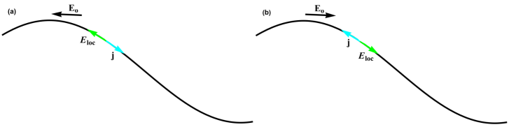
Figure 3: (a,b) Sketch of a cross-section of a bump on a wire surface by a plane that is parallel to a wire axis. A projection of a constant electric field $E_{0}$ onto a surface, $E_{loc}$, drives the electromigration adatom flux $j$ in the opposite direction, i.e. in the direction of the electron flow $j_{e}$. This contributes to either (a) a bump smoothing (stabilization), or to (b) a bump growth (destabilization).

Remark. In Ref. [18], where electromigration is not considered, a correction to $k_{c}(0)$ is derived that accounts for the finite perturbation amplitude, i.e. the starting assumption $\xi_{0}\ll 1$ is replaced by $0<\xi_{0}<1$. The corrected expression reads $k_{c}(0)=\sqrt{1+\xi_{0}^{2}}$. For the analyzes that follow in Sections III and IV it is not necessary to likewise correct $k_{c}$ in Eq. 5, since in Sec. III $k\rightarrow 0$ (is tiny) and $k_{c}$ is irrelevant, and in Sec. IV $k_{c}$ is not needed explicitly.

III Weakly nonlinear analysis slightly above the instability threshold $(k,E)=(0,E_{c})$

We start by substituting $r=1+\delta\xi(t,y),\ \delta\ll 1$ in the right-hand side of Eq. (1), expanding to second order in $\delta$, and formally adding the coefficients of $\delta$ and $\delta^{2}$. This results in:

$$\left(\alpha_{3}-1\right)\xi_{t} = -\left(E\alpha_{2}+\frac{1}{2}(\alpha_{1}+\alpha_{3})\right)\xi_{yy}-\frac{1}{2}(\alpha_{1}+\alpha_{3})\xi_{yyyy}+\frac{1}{2}(\alpha_{1}+\alpha_{3})\xi_{y}^{2}-\frac{1}{2}(\alpha_{1}+\alpha_{3})\xi_{yy}^{2}$$ (6)

$$- (\alpha_{1}+\alpha_{3})\xi_{y}\xi_{yyy}+\left[(E\alpha_{2}+\alpha_{1}+\alpha_{3})\xi+\left(2\alpha_{2}-\frac{1}{2}E(5\alpha_{1}+\alpha_{3})\right)\xi_{y}+\alpha_{2}\xi_{yyy}\right]\xi_{yy}+\alpha_{2}\xi_{y}\xi_{yyyy}.$$

LSA results (4), (5) may be recovered from Eq. (6).

Let $E=E_{c}+\epsilon E_{1},E_{1}=\mathcal{O}(1)>0$. Note that the coefficient of $\xi_{yy}$ changes its sign at $E=E_{c}$, hence it is proportional to $E-E_{c}=\epsilon E_{1}$, which is $\mathcal{O}(\epsilon)$. The balance of the largest nonlinear term $\sim\xi_{y}^{2}$ with the linear term $\sim\epsilon\xi_{yy}$ is for $\xi(t,y)=\epsilon\phi(t,y),\phi=\mathcal{O}(1)$. Also, since the linear instability interval is $0<k<k_{c}$, where $k_{c}=\sqrt{1+\frac{2\alpha_{2}E}{\alpha_{1}+\alpha_{3}}}=\sqrt{1-\frac{E}{E_{c}}}=\sqrt{\frac{-E_{1}}{E_{c}}\epsilon}=\mathcal{O}\left(\epsilon^{1/2}\right)$, the appropriate rescaling of the axial coordinate $y$ is $Y=\epsilon^{1/2}y$.

Thus also let:

$$\xi=\epsilon\phi;\quad T=\epsilon^{2}t\Leftrightarrow\partial_{t}=\epsilon^{2}\partial_{T},\quad Y=\epsilon^{1/2}y\Leftrightarrow\partial_{y}=\epsilon^{1/2}\partial_{Y},$$ (7)

where $T,Y$ are a slow time and a stretched axial variable.

Inserting $E=E_{c}+\epsilon E_{1}$ and expansions (7) in Eq. (6) we get:

$$\phi_{T}\epsilon^{3}=-\left\{\alpha_{2}E_{c}+\frac{1}{2}\left(\alpha_{1}+\alpha_{3}\right)\right\}\phi_{YY}\epsilon^{2}+\left\{-a\phi_{YY}-b\left[\phi_{YYYY}-\phi_{Y}^{2}-\phi\phi_{YY}\right]\right\}\epsilon^{3}+\mathcal{O}\left(\epsilon^{7/2}\right),$$ (8)

where $a=\frac{\alpha_{2}E_{1}}{\alpha_{3}-1}=\frac{SE_{1}\sin{2\psi}}{1+S}=E_{1}/4>0$, $b=\frac{\alpha_{1}+\alpha_{3}}{2\left(\alpha_{3}-1\right)}=\frac{2+S(1+\cos{2\psi})}{2(1+S)}\approx 0.966$. Noticing that the coefficient of $\phi_{YY}\epsilon^{2}$ is zero, in the lowest order $\epsilon^{3}$ we get the amplitude equation that resembles the famed Kuramoto-Sivashinsky (KS) equation, $\phi_{T}=-\phi_{YY}–\phi_{YYYY}-\phi_{Y}^{2}$:

$$\phi_{T}=-a\phi_{YY}-b\left[\phi_{YYYY}-\phi_{Y}^{2}-\phi\phi_{YY}\right].$$ (9)

It can be seen that Eq. (9) has the term $b\phi\phi_{YY}$ that is absent in KS equation, also the sign of $\phi_{Y}^{2}$ term is the opposite of the one in KS equation. This sign can be inverted by making the replacement $\phi\to-\phi$, thus it does not make a difference for the dynamics. However, $b\phi\phi_{YY}$ term changes the solutions and their dynamics qualitatively, as will be discussed shortly. Eq. (9) can be also written in the form:

$$\phi_{T}=-a\phi_{YY}-b\phi_{YYYY}+\frac{1}{2}b\ \partial_{YY}\phi^{2}.$$ (10)

Introducing the scalings of $Y$ and $T$:

$$X=\sqrt{\frac{a}{2b}}Y\Leftrightarrow\partial_{Y}=\sqrt{\frac{a}{2b}}\partial_{X},\quad\tau=\frac{a^{2}}{2b}T\Leftrightarrow\partial_{T}=\frac{a^{2}}{2b}\partial_{\tau}$$ (11)

eliminates one parameter from Eq. (10) and results in equation that has the form of Eq. (9) in Ref. [24]:

$$\phi_{\tau}=-\phi_{XX}-\frac{1}{2}\phi_{XXXX}+c\ \partial_{XX}\phi^{2},\quad c=\frac{b}{2a}.$$ (12)

Letting $\phi=h_{X}$ in Eq. (12) gives equation

$$h_{\tau}=-h_{XX}-\frac{1}{2}h_{XXXX}+c\ \partial_{X}h_{X}^{2},$$ (13)

that has the form of Eq. (8) in Ref. [24]. LSA of Eqs. (12) and (13) about the base states $\phi=1$ and $h_{X}=1$, respectively, give the perturbation growth rate $\omega=(1-2c)k^{2}-\frac{k^{4}}{2}$. Thus these base states are longwave unstable at $0<c<1/2\Leftrightarrow 0<b/a<1$, with the instability cut-off wavenumber $k_{c}=\sqrt{2(1-2c)}$.

Notice that setting $\phi=w_{XX},c=1$ in Eq. (12) and integrating twice with respect to $X$ gives $w_{\tau}=-w_{XX}-w_{XXXX}+w_{XX}^{2}$ [25]. This equation was rigorously studied in Ref. [26] (see equation (1D MKS) on p. 377 of that paper, which reads $w_{\tau}=-w_{XX}-w_{XXXX}+(1-\lambda)w_{X}^{2}+\sigma\lambda w_{XX}^{2}$, with $\lambda=\sigma=1$). For 1D MKS equation on a periodic domain these authors proved that depending on the stability of the trivial solution, either: (i) if it is unstable, there exist arbitrarily small initial perturbations that lead to a solution blow-up in a finite time, or (ii) if it is stable, there exist finite-amplitude initial perturbations that lead to a finite-time blow-up. These singularities exhibit self-similar structure in $w_{XX}$. Their numerical results indicated that $w$ generically becomes pointwise infinite at a finite time. Notice that the limit $\lambda\rightarrow 0$ recovers the KS equation which does not exhibit blow-up in one dimension. Also, Eq. (12) with the $-1$ coefficient of $\phi_{XXXX}$ and $c=-1$ has been studied in Ref. [27]. For that equation (the Sivashinsky equation) these authors found an infinite family of self-similar blow-up solutions, performed their LSA, and identified a unique stable blow-up solution. We will refer to Eq. (12) also as Sivashinsky equation.

A convenient scaling analysis of a solution singularity development for Eq. (12) (and Eq. (13)) was performed in Ref. [24]. Using directly the results of that analysis, we obtain that a downward spike in $\phi$ develops that is centered at the point $X(\tau)$; the depth of the spike increases as $\left(\tau_{s}-\tau\right)^{-1/2}$ and its width decreases as $\left(\tau_{s}-\tau\right)^{1/4}$ as $\tau$ approaches $\tau_{s}$ from below. Here $\tau_{s}$ is the time of a singularity formation (the blow-up time). In terms of the original variables:

$$\mbox{spike depth}=\frac{c_{1}}{\left(E-E_{c}\right)\sqrt{b\left(t_{s}-t\right)}},$$ (14)

$$\mbox{spike width}=c_{2}\sqrt{a\left(E-E_{c}\right)}\left(\frac{t_{s}-t}{b}\right)^{1/4},$$ (15)

$$\mbox{spike center displacement from}\ y=0=\frac{c_{3}\sqrt{a\left(E-E_{c}\right)}}{b^{1/4}}\left[t_{s}^{1/4}-\left(t_{s}-t\right)^{1/4}\right],$$ (16)

where the time of a singularity formation $t_{s}$ and the proportionality constants $c_{1,2,3}$ can’t be determined from the scaling analysis. Obviously, one expects that $t_{s}=t_{s}(E-E_{c})\equiv t_{s}(\Delta E)$, thus Eqs. (14)-(16) show the dependence of the spike parameters on time, but not yet on $\Delta E$. In order to find the latter functional dependence, first, we notice that the computation of Eq. (12) results in $\tau_{s}\sim 40$ (Fig. 4(a)). Thus using Eqs. (7) and (11):

$$t_{s}=\frac{2b\tau_{s}}{a^{2}\epsilon^{2}}=\frac{2bE_{1}^{2}\tau_{s}}{a^{2}\left(E-E_{c}\right)^{2}}=\frac{32\tau_{s}}{\left(E-E_{c}\right)^{2}}\sim 1300/\left(E-E_{c}\right)^{2}\sim 1.3\times 10^{7}$$ (17)

at $a=2,b=1,E_{1}=8\Leftrightarrow c=1/4$ and a representative value $\Delta E=0.01$. Evolution of the spike dimensions at these (fixed) values of $\Delta E$ and $t_{s}$ is shown in Fig. 4(b). It is seen that in comparison to the singularity of the width and the displacement, the singularity of the depth develops abruptly.

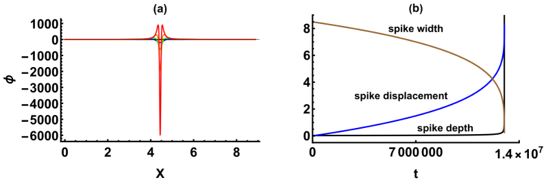
Figure 4: (a) Spike formation via computation of Eq. (12) with $c=1/4$. The initial condition is a small Gaussian-shaped perturbation of the base state $\phi=1$ on the interval $0\leq X\leq 2\sqrt{2}\pi$, where $2\sqrt{2}\pi$ is the most dangerous instability wavelength (the one at which the growth rate $\omega$ is the maximum value). Boundary conditions are periodic. The last shown profile corresponds to $\tau_{s}=43.35$. (b) Evolution of the spike dimensions (Eqs. (14)-(16)) at $\Delta E=0.01,a=2,b=1,E_{1}=8,t_{s}=1.3\times 10^{7}$. Proportionality constants $c_{1,2,3}=1$ are chosen to facilitate plotting three functions on the same screen.

Next, inserting $t_{s}=2bE_{1}^{2}\tau_{s}/a^{2}\left(E-E_{c}\right)^{2}$ in Eqs. (14)-(16) gives the following forms for the dependence of the spike parameters on $\Delta E$ and $t$:

$$\mbox{spike depth}=\frac{c_{1}a}{b\sqrt{2E_{1}^{2}\tau_{s}-\frac{a^{2}\left(E-E_{c}\right)^{2}t}{b}}},$$ (18)

$$\mbox{spike width}=c_{2}\left(2E_{1}^{2}\tau_{s}-\frac{a^{2}\left(E-E_{c}\right)^{2}t}{b}\right)^{1/4},$$ (19)

$$\mbox{spike center displacement from}\ y=0=c_{3}\left[\left(2\tau_{s}\right)^{1/4}\sqrt{E_{1}}-\left(2E_{1}^{2}\tau_{s}-\frac{a^{2}\left(E-E_{c}\right)^{2}t}{b}\right)^{1/4}\right].$$ (20)

Figure 5 shows the major spike dimension, its depth, as the contour plot of the two-variable function (18). Spike depth increases as the time and $\Delta E$ increase. Moreover, unless the time is close to a blow-up and $\Delta E$ is not very small, the depth is more sensitive to $\Delta E$ change than to $t$ change. This is the signature of a product $\left(E-E_{c}\right)^{2}t$ in Eq. (18), where the exponent of $t$ is one, and the exponent of $\Delta E$ is two. Same is true for the spike width and displacement.

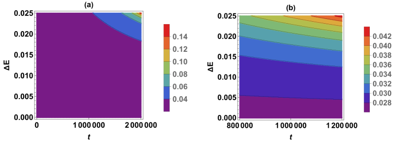
Figure 5: Spike depth, as given by Eq. (18). $a=2,b=1,E_{1}=8,\tau_{s}=40,c_{1}=1$. (b) is the zoom view of (a) in the middle of the time interval.

Also it is useful to expand Eq. (18) for small $\Delta E$ and $t$:

$$\mbox{spike depth}=\frac{c_{1}a}{bE_{1}\sqrt{2\tau_{s}}}+\frac{c_{1}a^{3}}{4\sqrt{2}b^{2}E_{1}^{3}\tau_{s}^{3/2}}\left(E-E_{c}\right)^{2}t+O\left(\left(E-E_{c}\right)^{4}t^{2}\right).$$ (21)

This shows that the spike depth grows quadratically in $\Delta E$ and only linear in $t$.

IV A weakly nonlinear multi-scale analysis of the primary modes of instability

As was already noted in Introduction, due to nonlinearity of a governing PDE (1) very shortly after the initiation of a morphological instability the initial sinusoidal, single-harmonic form of a solution (the initial condition) ceases to exist, and the solution is represented by a Fourier series. Without a loss of generality, we will account only for a handful of major terms in that series, i.e. the sinusoidal terms having a wavenumbers that are a small integer multiples of a wavenumber of the primary mode (the sinusoidal initial condition/perturbation) [18], and derive their time-dependent amplitudes. The primary mode has a finite wavenumber $0<k<k_{c}$.

We start with the following ansatz for the perturbation of the base state $r=1$:

$$r=1+\epsilon r_{1}\left(t_{0},t_{1},t_{2};E\right)\cos{ky}+\epsilon r_{4}\left(t_{0},t_{1},t_{2};E\right)\sin{ky}+\epsilon^{2}r_{2}\left(t_{0},t_{1},t_{2};E\right)\cos{2ky}+\epsilon^{2}r_{3}\left(t_{0},t_{1},t_{2};E\right)\sin{2ky},\ \epsilon\ll 1$$ (22)

where $t_{0}$ is the fast time and $t_{1},t_{2}$ are the slow times. Thus the time derivative reads:

$$\frac{\partial}{\partial t}=\frac{\partial}{\partial t_{0}}+\epsilon\frac{\partial}{\partial t_{1}}+\epsilon^{2}\frac{\partial}{\partial t_{2}}.$$ (23)

The initial conditions are chosen as:

$$r_{1}\left(0,t_{1},t_{2};E\right)=\xi_{0},\;0<\xi_{0}<1;\quad r_{2,3,4}\left(0,t_{1},t_{2};E\right)=0.$$ (24)

Now we proceed according to this plan: substitute the expansions (22) and (23) in Eq. (1), collect the terms of the same powers of $\epsilon$ on each of the two sides of the equation and equate them; next, for each of the resulting statements, collect the terms proportional to $\cos{ky}$, $\sin{ky}$, $\cos{2ky}$, and $\sin{2ky}$ on each of the two sides of a statement and equate, separately, the coefficients of these harmonics.

At the order $\epsilon$ we get:

$$\frac{\partial r_{1}}{\partial t_{0}}\cos{ky}+\frac{\partial r_{4}}{\partial t_{0}}\sin{ky}=\sigma(k;E)r_{1}\cos{ky}+\sigma(k;E)r_{4}\sin{ky},$$ (25)

thus

$$\frac{\partial r_{1,4}}{\partial t_{0}}=\sigma(k;E)r_{1,4},$$ (26)

where the growth rate $\sigma(k;E)$ is given by Eq. (4).

At the order $\epsilon^{2}$ we get:

$$\frac{\partial r_{1}}{\partial t_{1}}\cos{ky}+\frac{\partial r_{4}}{\partial t_{1}}\sin{ky}+\frac{\partial r_{2}}{\partial t_{0}}\cos{2ky}+\frac{\partial r_{3}}{\partial t_{0}}\sin{2ky}=f_{1}\left(k,r_{1},r_{4};E\right)+f_{2}\left(k,r_{1},r_{4},r_{2};E\right)\cos{2ky}+f_{3}\left(k,r_{1},r_{4},r_{3};E\right)\sin{2ky},$$ (27)

where $f_{1,2,3}$ are certain complicated functions. Therefore:

• $$\frac{\partial r_{1,4}}{\partial t_{1}}=0\rightarrow r_{1,4}=r_{1,4}\left(t_{0},t_{2};E\right).$$ (28)

  Applying the initial conditions (24) and accounting for Eq. (28) we get from the linear ODE (26):

  $$r_{1}=r_{1}\left(t_{0};E\right)=\xi_{0}e^{\sigma(k;E)t_{0}},\quad r_{4}=0.$$ (29)

  It can be observed now that the LSA result of Sec. II.1 for the primary mode has been obtained at the linear stage (at order $\epsilon$) of a multi-scale expansion.

• Substituting $r_{4}=0$ in $f_{2}$ and $f_{3}$, for $r_{2}$ and $r_{3}$ from Eq. (27) one obtains the linear ODEs:

  $$\frac{\partial r_{2,3}}{\partial t_{0}}=f_{2,3}\left(k,r_{1},r_{2,3};E\right)=p(k;E)r_{2,3}+q_{2,3}(k;E)r_{1}\left(t_{0};E\right)^{2},$$ (30)

  where

  $$p(k;E)=2\frac{2+S(1+\cos{2\psi})}{1+S}k^{2}\left(1-4k^{2}\right)+4E\frac{S\sin{2\psi}}{1+S}k^{2}=4\sigma(k;E)-6\frac{2+S(1+\cos{2\psi})}{1+S}k^{4},$$ (31)

  $$q_{2}(k;E)=-3\frac{2+S(1+\cos{2\psi})}{4(1+S)}k^{2}\left(1+k^{2}\right)-E\frac{S\sin{2\psi}}{2(1+S)}k^{2},$$ (32)

  $$q_{3}(k;E)=\frac{S\sin{2\psi}}{1+S}k^{3}\left(1-k^{2}\right)+E\frac{S^{2}(\cos{4\psi}-1)-S(6\cos{2\psi}+10)-12}{4(1+S)}k^{3}.$$ (33)

  Substituting $r_{1}\left(t_{0};E\right)$ from Eq. (29) and taking into account the initial conditions, the solutions of Eqs. (30) read:

  $$r_{2,3}=r_{2,3}\left(t_{0};E\right)=\frac{q_{2,3}(k;E)\xi_{0}^{2}}{p(k;E)-2\sigma(k;E)}\left[\exp{\left(p(k;E)t_{0}\right)}-\exp{\left(2\sigma(k;E)t_{0}\right)}\right].$$ (34)

• Finally, for consistency of Eq. (27) one needs $f_{1}\left(k,r_{1};E\right)=0$. This gives the constraint $k^{2}\left(k^{2}-k_{c}^{2}\right)r_{1}\left(t_{0};E\right)^{2}=0$, where $k_{c}$ is seen in Eq. (5). Since $r_{1}\left(t_{0};E\right)\neq 0$, either $k=0$, or $k=k_{c}$. This implies that the results would formally apply only at the longwave instability threshold $k=0$, or at the shortwave instability cut-off wavenumber $k_{c}$. However, we reasonably assume that the constraint holds approximately at $k=\delta_{1}$ and $k=k_{c}-\delta_{2}$, where $\delta_{1,2}$ are a positive constants that quantify the deviation from these values into the instability interval $0<k<k_{c}$. In particular, $k=\delta_{1}$ is the most dangerous wavenumber in LSA when $\delta_{1}=k_{c}/\sqrt{2}$.

Figure 6 shows $r_{1}$ as the function of the electric field at fixed $t_{0}$ and at various distances $\delta$ from the longwave instability threshold $k=0$ and from the short-wave instability cut-off $k=k_{c}$. For this, we took $\delta_{1}=\delta_{2}=\delta$ and substituted $k=\delta$ and $k=k_{c}-\delta$ in Eq. (29), where $\sigma(k;E)$ and $k_{c}(E)$ are given by Eqs. (4), (5). In the former case (Fig. 6(b)) one can see that $r_{1}\sim c_{1}\exp{(c_{2}E)},c_{1},c_{2}=const.$, and values of these constants can be easily calculated. However, for the particular numerical values of the parameters and for the plotting interval these exponential curves are well approximated by the straight lines. In the latter case (Fig. 6(a)) the analytical dependence on $E$ is complicated, but the curve data can be fitted: $\delta=0.001$: $r_{1}=0.00997+0.000048\exp{(0.145717E)}$; $\delta=0.01$: $r_{1}=0.00973+0.000458\exp{(0.153945E)}$; $\delta=0.025$: $r_{1}=0.00941+0.001056\exp{(0.16734E)}$.

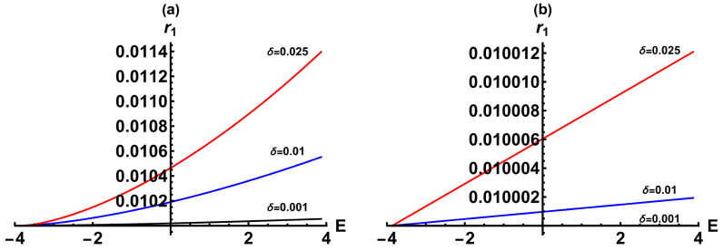
Figure 6: The amplitude of $\cos{ky}$ term in the ansatz (22), given by Eq. (29), at $t_{0}=1$, $\xi_{0}=0.01$ for $E_{c}+0.01\leq E\leq-E_{c}$, where $E_{c}=-3.866$. (a) Near the short-wave instability cut-off; (b) Near the long-wave instability threshold.

A close look at $r_{2}(E)$ and $r_{3}(E)$ curves (Fig. 7) and the comparison to $r_{1}(E)$ in Fig. 6 shows, first, that $r_{1}$ is several orders of magnitude larger than $r_{2,3}$. Thus the primary mode $\cos{ky}$ is dominant in the spectrum, as expected [18]. Next, the absolute values of $r_{2}$ are two orders of magnitude larger than the absolute values of $r_{3}$ near the longwave instability threshold, while the converse is true near the short-wave instability cut-off. Therefore $\cos{2ky}$ and $\sin{2ky}$ are the next two fast growing modes in the spectrum.

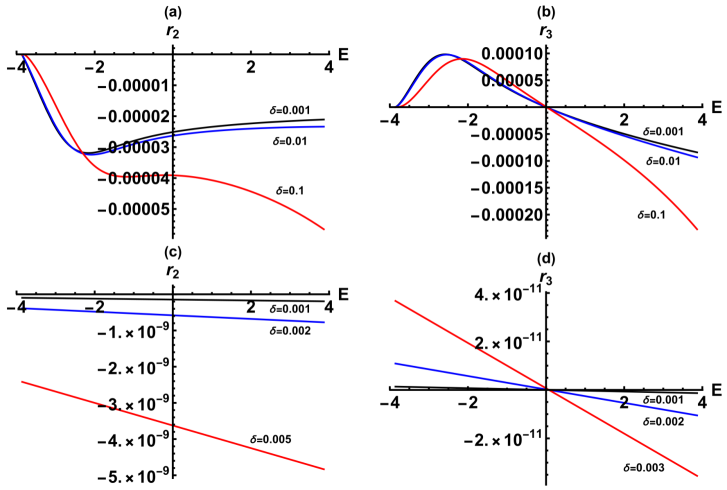
Figure 7: The amplitudes of $\cos{2ky}$ and $\sin{2ky}$ terms in the ansatz (22), given by Eqs. (34), at $t_{0}=1$, $\xi_{0}=0.01$ for $E_{c}+0.01\leq E\leq-E_{c}$, where $E_{c}=-3.866$. (a,b) Near the short-wave instability cut-off; (c,d) Near the long-wave instability threshold.

The largest of $r_{2,3}$ amplitudes, $r_{3}$, is plotted in Fig. 8 vs. $t_{0}$ and $E$ near the short-wave instability cut-off. Cross-secting Fig. 8(a) by a vertical cut shows that at any fixed $t_{0}$ the amplitude dependence on $E$ is roughly as seen in Fig. 7(b). Moreover, a (positive) maximum of the amplitude increases with $t_{0}$, as seen in Fig. 8(b).

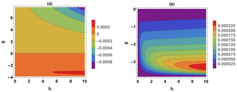
Figure 8: The amplitude of $\sin{2ky}$ term in the ansatz (22), given by Eqs. (34), at $\xi_{0}=0.01$, near the short-wave instability cut-off. (b) is the zoom view of the bottom region in (a).

V Summary

Provided that the electric field slightly exceeds a threshold value that is necessary for initiation of a morphological instability, the weakly nonlinear analysis that we carried out shows for the first time the electric field-and-time dependence of the dimensions of the shallow spike, whose strongly nonlinear development would ultimately lead to a wire pinch-off and its breakup into a chain of nanoparticles. In particular, this analysis shows that the spike depth initially grows quadratically in the deviation from a threshold value of the electric field. For the initial surface perturbation of the form $\xi_{0}\cos{ky},\;0<\xi_{0}<1$ (where $y$ is the axial variable) a separate, multi-scale analysis of a weakly nonlinear phase of the instability shows that in that regime the fastest growing instability modes are $\cos{ky}$, $\cos{2ky}$, and $\sin{2ky}$, and for these modes we found the explicit dependence of their amplitudes on time and the strength of the applied electric field.

VI Acknowledgments

The author thanks Alexander A. Nepomnyashchy and Mark R. Bradley for very useful suggestions and discussions regarding the analysis in Sec. III. Mark R. Bradley is also acknowledged for bringing his paper [24] to author’s attention and for pointing to Ref. [26].

References

- [1] H.B. Huntington, Ch. 6: Electromigration in metals, in: Diffusion in Solids: Recent Developments, Ed. A.S. Nowick, Academic Press, 1975.
- [2] P.S. Ho and T. Kwok, “Electromigration in metals”, Rep. Prog. Phys. 52, 301-348 (1989).
- [3] P.J. Rous, T.L. Einstein, and E.D. Williams, “Theory of surface electromigration on metals: application to self-electromigration on Cu(111)”, Surf. Sci. 315, L995-L1002 (1994).
- [4] Hongkun Park, Andrew K. L. Lim, A. Paul Alivisatos, J. Park, and Paul L. McEuen, “Fabrication of metallic electrodes with nanometer separation by electromigration”, Appl. Phys. Lett. 75, 301 (1999).
- [5] L. Valladares, L.L. Felix, A.B. Dominguez, T. Mitrelias, F. Sfigakis, S.I. Khondaker, C.H.W. Barnes, and Y. Majima, “Controlled electroplating and electromigration in nickel electrodes for nanogap formation”, Nanotechnology 21, 445304 (2010).
- [6] L. Arzubiaga, F. Golmar, R. Liopis, F. Casanova, and L.E. Hueso, “Tailoring palladium nanocontacts by electromigration”, Appl. Phys. Lett. 102, 193103 (2013).
- [7] R. Hoffmann-Vogel, “Electromigration and the structure of metallic nanocontacts”, Appl. Phys. Rev. 4, 031302 (2017).
- [8] F.A. Nichols and W.W. Mullins, “Surface-(Interface-) and volume-diffusion contributions to morphological changes driven by capillarity”, Trans. Metall. Soc. AIME 233, 1840–1848 (1965).
- [9] F.A. Nichols and W.W. Mullins, “Morphological Changes of a Surface of Revolution due to Capillarity Induced Surface Diffusion”, J. Appl. Phys. 36, 1826 (1965).
- [10] J.W. Cahn, “Stability of rods with anisotropic surface free energy”, Scripta Metall. 13, 1069–1071 (1979).
- [11] A.J. Bernoff, A.L. Bertozzi, and T.P. Witelski, “Axisymmetric surface diffusion: dynamics and stability of self-similar pinchoff”, J. Stat. Phys. 93 725–776 (1998).
- [12] B.D. Coleman, R.S. Falk, and M. Moakher, “Stability of cylindrical bodies in the theory of surface diffusion”, Physica D 89, 123-135 (1995).
- [13] M.S. McCallum, P.W. Voorhees, M.J. Miksis, S.H. Davis, and H. Wong, “Capillary instabilities in solid thin films: Lines”, J. Appl. Phys. 79, 7604 (1996).
- [14] H. Wong, M.J. Miksis, P.W. Voorhees, and S.H. Davis, “Universal pinch off of rods by capillarity-driven surface diffusion”, Scripta Mater. 39, 55–60 (1998).
- [15] D.J. Kirill, S.H. Davis, M.J. Miksis, and P.W. Voorhees, “Morphological instability of a whisker”, Proc. R. Soc. Lond. A 455, 3825-3844 (1999).
- [16] K.F. Gurski, and G.B. McFadden, “The effect of anisotropic surface energy on the Rayleigh instability”, Proc. R. Soc. Lond. A 459 2575–2598 (2003).
- [17] K.F. Gurski, G.B. McFadden, and M.J. Miksis, “The effect of contact lines on the Rayleigh instability with anisotropic surface energy”, SIAM J. Appl. Math. 66, 1163–1187 (2006).
- [18] F. Wang, O. Tschukin, T. Leisner, H. Zhang, B. Nestler, M. Selzer, G.C. Marques, and J. Aghassi-Hagmann, “Morphological stability of rod-shaped continuous phases”, Acta Materialia 192, 20-29 (2020).
- [19] V. Gorshkov and V. Pivman, “Kinetic Monte Carlo model of breakup of nanowires into chains of nanoparticles”, J. Appl. Phys. 122, 204301 (2017).
- [20] M. Khenner, “Effect of electromigration on onset of morphological instability of a nanowire”, J. Eng. Math. 140, 6 (2023).
- [21] M. Khenner, “Nanowire breakup via a morphological instability enhanced by surface electromigration”, Modelling and Simulation in Materials Science and Engineering 32, 015003 (2024).
- [22] T.F. Marinis, R.F. Sekerka, F.D. Lemkey, H.E. Cline, and M. McLean, In-Situ Composites IV, Elsevier, NY, pp. 315-327 (1982).
- [23] M. Schimschak and J. Krug, “Surface electromigration as a moving boundary value problem”, Phys. Rev. Lett. 78, 278 (1997).
- [24] M.P. Gelfand and R.M. Bradley, “One dimensional conservative surface dynamics with broken parity: Arrested collapse versus coarsening”, Physics Letters A 379, 199–205 (2015).
- [25] R.M. Bradley, private communication.
- [26] A.J. Bernoff and A.L. Bertozzi, “Singularities in a modified Kuramoto-Sivashinsky equation describing interface motion for phase transition”, Physica D 85, 375-404 (1995).
- [27] A.J. Bernoff and T.P. Witelski, “Stability and dynamics of self-similarity in evolution equations”, J. Eng. Math. 66, 11-31 (2010).