The effects of a minimal length on the Kerr metric and the Hawking temperature

Abstract

A brief review of the pseudo complex General Relativity (pcGR) will be presented, with its consequences, as the accumulation of a dark energy around a mass and a generalized Mach’s principle. The main objective in this contribution is to determine the Hawking temperature and the Entropy for various limits: i) The pc-Schwarzschild case with no minimal length present, ii) the pc-Kerr metric without a minimal length and iii) the general case, the pc-Kerr metric with a minimal length present. The physical consequences of a minimal length will be discussed, a possible interpretation of a gravitational Schwinger effect and the appearance of negative temperature. For large masses a minimal length does not show any sensible effect, but only for very small masses, several orders of the Planck mass, where non-trivial effects emerge, important for the production of mini-black holes in the early universe. Our results are more general than being restricted to pcGR. Any other model which assumes a distribution of dark energy around a stellar body produces the same effects. In contrast to these models, pcGR demands the presence of a dark energy term.

1 Introduction

In [1] the pseudo-complex algebraic extension of the General Relativity (GR) was introduced, called pseudo complex General Relativity (pcGR). The main consequences of this theory are the mandatory appearance of a dark energy term on the right hand side of the Einstein equation and the existence of a minimal length. The accumulation of dark energy around stellar object implies a generalized Mach’s principle, namely that any mass not only curves space-time but also modifies the vacuum structure around it.

In [2] the theory was explained in detail with the pc-Schwarzschild, pc-Kerr metric and applications were presented, as to the description of neutron stars and the accretion disk structure around a black hole. In [3] the pcGR was put into relation to several algebraic extensions of the GR, showing that all versions are contained as special cases of pcGR. Accretion disks around a black hole were investigated [2, 3, 4] and it was shown that deviations from GR only appear very near to the event horizon. A dark ring in the accretion, followed by a bright one is predicted, however, an observable resolution of minimal $5\mu as$ are required, not achieved up to now. Another consequence of this theory is that any mass can be stabilized, though very heavy objects still resemble black holes as predicted by the GR. Nevertheless, some possible emissions of light, due to in-falling matter, at/near the poles is predicted [5]. Therefore, pcGR predicts that stellar objects larger than 2.3 solar masses will be observed which neither behave as neutron stars nor as black holes, the transition to stellar objects resembling black holes will be fluent.

In this contribution, we are interested in determining the Hawking temperature and the entropy of these stellar objects, as a function of the rotational Kerr parameter $a$ and $b$, the last describing the accumulation of dark energy around a stellar object. We also propose that all space outside a stellar object is subject to a Hawking radiation, similar to the Schwinger effect known in Quantum Electrodynamics (QED) [6]. Another interest is to study the effects of a minimal length on this radiation. The pcGR will show that when an event horizon is present, near to this horizon negative temperatures will appear, which correspond to negative pressure [7], thus, stabilizing the star.

The paper is organized as follows: In Section 2 the pcGR is resumed and its main consequences listed. In Section 3 the application to the Kerr metric is discussed in several steps. First the limit of a non-rotating stellar object with no minimal length is investigated, after that the Kerr metric with no minimal length is considered and finally the general case, a rotating stellar object with a minimal length present. The last case will show dramatic effects near the event horizon In Section 4 Conclusions are drawn.

2 Pseudo-complex General Relativity

In this section, we will resume the theory of pcGR, i.e., its motivation, structure and some important consequences. The presentation will unite several results which have been published separately, but are important for a complete picture.

One possible manner to modify GR is an algebraic extension [3]. With that notion we associate the use of alternative variables than $x^{\mu}$, with $\mu$ = 0, 1, 2, 3. However, not all algebraic extensions are consistent, as noted in [8]: Most algebraic extensions lead in the limit of weak gravitational fields to the existence of ghost and/or tachyon solutions. Only two sets of coordinates are without problems, namely the real coordinates $(x^{\mu})$, which are the standard coordinates in GR, and the pseudo-complex coordinates

$$X^{\mu} = x^{\mu}+Iy^{\mu}~{}~{}~{},$$ (1)

with $I^{2}=1$ and $y^{\mu}$, yet to be determined. Thus, the space in pc-GR is 8-dimensional and one has to find a procedure to reduce it again to a 4-dimensional space, which will be exactly what will be explained further below through the use of a constraint.

Alternatively to (1) the $X^{\mu}$ can be expressed in terms of newly defined operators $\sigma_{\pm}=\frac{1}{2}\left(1\pm I\right)$, i.e.,

$$X^{\mu} = X^{\mu}_{+}\sigma_{+}+X^{\mu}_{-}\sigma_{-}$$

$$\sigma_{\pm}^{2} = \sigma_{\pm}~{},~{}\sigma_{+}\sigma_{-}=0~{},~{}\sigma_{+}+\sigma_{-}~{}=~{}1~{},~{}\sigma_{+}-\sigma_{-}~{}=~{}I$$

$$X^{\mu} = \frac{1}{2}\left(x^{\mu}\pm y^{\mu}\right)~{}~{}~{},$$ (2)

which provides a division of $X^{\mu}$ in terms of the zero-divisor components of $\sigma_{\pm}$. The notion of a zero divisor is a consequence of the property $\sigma_{+}\sigma_{-}=0$, i.e., two numbers $\lambda_{+}\sigma_{+}$ and $\lambda_{-}\sigma_{-}$ multiplies gives zero, which shows that the pseudo-complex variables do not form a field but rather a ring.

The length element squared in pcGR has now the form

$$d\omega^{2} = g_{\mu\nu}(X)dX^{\mu}dX^{\nu}$$ (3)

$$= g^{+}_{\mu\nu}(X_{+})dX_{+}^{\mu}dX_{+}^{\nu}\sigma_{+}+g^{-}_{\mu\nu}(X_{-})dX_{-}^{\mu}dX_{-}^{\nu}\sigma_{-}$$

$$= \left\{g^{+}_{\mu\nu}(X_{+})dX_{+}^{\mu}dX_{+}^{\nu}+g^{-}_{\mu\nu}(X_{-})dX_{-}^{\mu}dX_{-}^{\nu}\right\}$$

$$+I\left\{g^{+}_{\mu\nu}(X_{+})dX_{+}^{\mu}dX_{+}^{\nu}-g^{-}_{\mu\nu}(X_{-})dX_{-}^{\mu}dX_{-}^{\nu}\right\}$$

$$= \left\{g^{S}_{\mu\nu}\left[dx^{\mu}dx^{\nu}+dy^{\mu}dy^{\nu}\right]+g^{A}_{\mu\nu}\left[dx^{\mu}dy^{\nu}+dy^{\mu}dx^{\nu}\right]\right\}$$

$$+I\left\{g^{A}_{\mu\nu}\left[dx^{\mu}dx^{\nu}+dy^{\mu}dy^{\nu}\right]+g^{S}_{\mu\nu}\left[dx^{\mu}dy^{\nu}+dy^{\mu}dx^{\nu}\right]\right\}~{}~{}~{},$$

with the symmetric and antisymmetric combinations of the metrics from the two zero divisior components:

$$g^{S}_{\mu\nu} = \frac{1}{2}\left(g^{+}_{\mu\nu}+g^{-}_{\mu\nu}\right)~{},~{}g^{A}_{\mu\nu}~{}=~{}\frac{1}{2}\left(g^{+}_{\mu\nu}-g^{-}_{\mu\nu}\right)~{}~{}~{}.$$ (4)

The length element has to be real (particles only move on a real trajectory) and, thus, demanding that the pseudo-imaginary component in (3) vanishes, represents a constraint which has to be implemented.

The equations of motion, i.e. the modified Einstein equations, are derived from a variational principle, at first sight to be identical to the one in GR, but in distinction all objects (tensors) are pseudo-complex (pc) [2, 3]. The action is defined as

$$S = \int dX^{4}\sqrt{-g}\left({\cal R}+2\alpha\right)$$ (5)

with ${\cal R}$ as the pc-Riemann scalar and the term $\alpha$ describes the an additional dark energy. In the first publication, where the pcGR was presented [1, 2], a different variational principle was proposed, which is more involved to implement. But already in the appendix in [2] the alternative proposal, to apply instead a constraint, was discussed.

Therefore, one imposes the variational principle $\delta S=0$ with a constraint, namely

$$\delta S = \delta S_{+}\sigma_{+}+\delta S_{-}\sigma_{-}~{}=~{}0$$

$$0 = \left(\sigma_{+}-\sigma_{-}\right)\left\{g^{+}_{\mu\nu}(X_{+})dX_{+}^{\mu}dX_{+}^{\nu}-g^{-}_{\mu\nu}(X_{-})dX_{-}^{\mu}dX_{-}^{\nu}\right\}$$ (6)

$$= I\left\{g^{A}_{\mu\nu}\left[dx^{\mu}dx^{\nu}+dy^{\mu}dy^{\nu}\right]+g^{S}_{\mu\nu}\left[dx^{\mu}dy^{\nu}+dy^{\mu}dx^{\nu}\right]\right\}~{}~{}~{},$$

varying with respect to $g^{+}_{\mu\nu}$ in the $\sigma_{+}$ zero-divisor component and with respect to $g^{-}_{\mu\nu}$ in the $\sigma_{-}$ zero-divisor component. The constraint is implemented via the use of a Lagrange multiplier $\lambda$ [4].

This variation leads to the modified Einstein equations [3]

$${\cal R}^{\pm}_{\mu\nu}-\frac{1}{2}g^{\pm}_{\mu\nu}{\cal R}_{\pm} = 8\pi T_{\pm~{}\mu\nu}^{\Lambda}~{}~{}~{},$$ (7)

with the energy momentum tensors in the zero-divisor basis given by

$$8\pi\kappa T_{\pm~{}\mu\nu}^{\Lambda} = \lambda u_{\mu}u_{\nu}+\lambda\left({\dot{y}}_{\mu}{\dot{y}}_{\nu}\pm u_{\mu}{\dot{y}}_{\nu}\pm u_{\nu}{\dot{y}}_{\mu}\right)+\alpha g_{\mu\nu}^{\pm}~{}~{}~{},$$ (8)

where the dot refers to the derivative with respect to the eigentime ($ds=d\tau$).

To introduce a constraint is paid with a price, namely to find a solution to this constraint.

From this, we conclude that using pc-coordinates leads to Einstein equations which demands the appearance of a non-zero energy-momentum tensor on the right hand side of the equations. At this point, we have to introduce a phenomenological ansatz, which is based on the observation that a curved space creates vacuum fluctuations [9, 10], resulting in an $\sim 1/r^{6}$ dependence, times a function in $r$. As shown in [10] these vacuum fluctuations diverge at the event horizon, which is probable a consequence of not taking into account back-reaction effects. Nevertheless, it shows that vacuum fluctuations are strong near the position of the event horizon and the dependence on the radial distance we take into account by a fall-off of the dark energy as $\sim\frac{1}{r^{6}}$. Lower powers are excluded by observation [3], but the fall-off can be stronger. In [3] the fall-off of the dark energy is parametrized as $1/r^{n}$.

In what follows we will show that after some justifiable approximations we are left with one set of real Einstein equations, with a non-zero energy-momentum tensor on its right hand side, and the solution of the constraint will lead to a dispersion relation, which in a flat space is the one known from special relativity. The two equations in (7) will, under the proposed approximations, fuse to one equation.

These approximations are: i) We assume that the metrics in the two zero-divisor component are exactly the same, namely

$$g^{\pm}(X_{\pm}) \approx g_{\mu\nu}(x)~{}~{}~{}.$$ (9)

This is equivalent to assume the same functional form of the metrics, i.e., $g^{\pm}(X_{\pm})=g(X_{\pm})$. ii) A further assumption is that the corrections to the minimal length in the metric are negligible, i.e., the dependence is only on the real variable $x^{\mu}$. This approximation also implies that

$$g^{S}_{\mu\nu}(x) = g_{\mu\nu}(x)~{}{\rm and}~{}g^{A}_{\mu\nu}(x)~{}=~{}0~{}~{}~{}.$$ (10)

With this, the constraint reduces to

$$g_{\mu\nu}(x)dx^{\mu}dy^{\nu} = 0~{}~{}~{}.$$ (11)

This is the generalized dispersion relation with the solution for $y^{\mu}$ given by

$$y^{\mu} = l\frac{Dx^{\mu}}{D\tau}~{}~{}~{},$$ (12)

with $D$ being the covariant derivative [11] and $\tau$ is the eigentime. The factor $l$ is introduced for dimensional reasons and has the dimension of length ($c=1$).

Here, we have an example of a theory which uses a minimal length as a parameter, i.e., it is not affected by a Lorentz transformation. All symmetries in GR are preserved in pcGR, which is a huge advantage. For the case of a flat space ($g_{\mu\nu}=\eta_{\mu\nu}$, with $\eta_{\mu\nu}$ the Minkowsky metric) the dispersion relation reduces to the standard one and the solution of $y^{\mu}$ is just $y^{\mu}=lu^{\mu}$, with $u^{\mu}$ as the 4-velocity. It is obtained directly from (12), noting that all Christophel symbols vanish in flat space. This is the standard assumption for $y^{\mu}$ in theories including a minimal length (maximal acceleration) [12, 13].

Using (10), the Einstein tensors $G^{\pm}_{\mu\nu}$, which are pure functions of the metric, are in both zero divisor component equal, yielding $G_{\mu\nu}$. The energy-momentum tensors are also set to $T^{\Lambda}_{\mu\nu}$ = $\frac{1}{2}\left(T^{\Lambda}_{+~{}\mu\nu}+T^{\Lambda}_{-~{}\mu\nu}\right)$ (exploiting the symmetry in the zero-divisor components), where we added the upper symbol $\Lambda$ in order to refer it to dark energy.

To resume, we are finally left with the equations

$$G_{\mu\nu} = 8\pi\kappa T^{\Lambda}_{\mu\nu}$$

$$y^{\mu}~{}=~{}\frac{Dx^{\mu}}{D\tau} \leftarrow g_{\mu\nu}dx^{\mu}dy^{\mu}=0$$

$$d\omega^{2} = g_{\mu\nu}(x)\left[dx^{\mu}dx^{\nu}+dy^{\mu}dy^{\nu}\right]~{}~{}~{}.$$ (13)

The ansatz for $T_{\mu\nu}$ is made using a phenomenological approach, based on results from semi-classical Quantum Mechanics [9, 10] and it was explained above.

A phenomenological parametrization is finally used, describing a falling-off of the dark energy density as a power in the radial distance. For a particular ansatz, please consult [3]

The main results of this section can be resumed as follows:

• The pc-extension of GR (pcGR) demands a non-zero energy-momentum tensor on the right hand side of the Einstein equations. This term is associated to the appearance of a vacuum with an internal structure, given by a dark energy. The main consequence is as follows:

• The pc-GR implies an extension of Mach’s principle, namely that Mass deforms not only space-time but also changes the vacuum properties around any mass. We denominate it as the extended Mach’s principle. This result may be important, giving hints on what a quantized Gravity has to include.

• The pcGR also has as a consequence the generalized dispersion relation, resulting in conditions for the four components of $y^{\mu}$. Thus, it describes how a particle moves in the 8-dimensional space, restricting it to a 4-dimensional embedded space.

• Another consequence of the constraint is the appearance of a minimal length parameter $l$. This parameter is a scalar and is not affected by a Lorentz transformation. It represents a huge advantage, compared to other theories with a physical minimal length, subject to Lorentz contraction. In addition, the appearance of a minimal length may shed, too, some light on what a quantized Gravity has to contain.

3 Application to the Schwarzschild and Kerr metric

Defining a dimensionless radial variable

$$y = \frac{r}{m}~{}~{}~{},$$ (14)

outside the star’s mass distribution, the non-zero components of the Kerr metric are [3]

$$g_{00} = -\frac{y^{2}-2y+a^{2}\cos^{2}\vartheta+\frac{b}{6y^{2}}}{y^{2}+a^{2}\cos^{2}\vartheta}~{}~{}~{},$$

$$g_{11} = \frac{y^{2}+a^{2}\cos^{2}\vartheta}{y^{2}-2y+a^{2}+\frac{b}{6y^{2}}}~{}~{}~{},$$

$$g_{22} = y^{2}+a^{2}\cos^{2}\vartheta~{}~{}~{},$$

$$g_{33} = (y^{2}+a^{2})\sin^{2}\vartheta+\frac{a^{2}\sin^{4}\vartheta\left(2y-\frac{b}{6y^{2}}\right)}{y^{2}+a^{2}\cos^{2}\vartheta}~{}~{}~{},$$

$$g_{03} = 2\frac{-a\sin^{2}\vartheta~{}2y+a\frac{b}{6y^{2}}\sin^{2}\vartheta}{y^{2}+a^{2}\cos^{2}\vartheta}~{}~{}~{},$$ (15)

where $b$ is the parameter for the size of accumulation of dark energy around a stellar object. These components change insside the stars’ mass distribution, which will not be considered here. For a possible path, please consult [14].

In order to calculate the position of the event horizon, we determine the zeros of the $g_{00}$ component, which is equal to solving the equation [17]

$$y^{4}-2y^{3}+a^{2}y^{2}+b/6 = 0~{}~{}~{},$$ (16)

with four solutions.

In what follows, several limits will be discussed, as the Schwarzschild solution ($a=0$) but no minimal length, the Kerr solution but still with $l=0$ and finally the most general case, including the minimal length. There, we will see that the minimal length has important consequences for the structure of small black holes.

3.1 Schwarzschild case, $a=0$ AND $l=0$

The basis of the following calculations is the Schwarzschild metric, obtained using $a=0$ in the Kerr metric (15).

For $b=0$ we arrive at the standard expression in General Relativity (GR). For $b=\frac{81}{8}$, we arrive at the value used in the pseudo-complex General Relativity (pcGR) [1, 3].

3.1.1 Hawking temperature

According to [15], the surface gravity $\kappa$, is obtained via

$$\kappa = \frac{1}{2}\frac{\partial g_{00}}{\partial r}~{}=~{}\frac{1}{2m}\frac{\partial g_{00}(y)}{\partial y}~{}~{}~{},$$ (17)

where it is important to note that $\kappa$ times the mass $m$ is only a function in $y$. The derivative is usually applied at the position of the event horizon. In [15] essentially the same method is applied. Here, we will also calculate the $\kappa$ at an arbitrary distances to the center. The reason lies in our assumption that pair creation may be possible as soon as there is a gravitational field [10, 16], of course for weak fields the yield would be negligible. The same assumption is used in Quantum Electrodynamics (QED) and this phenomenon is called the Schwinger effect [6], which we will denote as the gravitational Schwinger effect.

The Hawking temperature is related to the surface gravity via [9, 15]

$$T = \frac{\kappa}{2\pi}~{}=~{}\frac{1}{2\pi my_{h}^{2}}\left(1-\frac{b}{3y_{h}^{3}}\right)~{}~{}~{},$$ (18)

where the final result is given on the right hand side. The position $y$ is taken here at the event horizon. But, note that we also can calculate $T$ at arbitrary distances, where $y$ is used instead of $y_{h}$. In Fig. 1 the temperature at the event horizon is plotted versus b. Note, that $T$ times the mass $m$ is only a function in $y$, only valid outside the star’s mass distribution, i.e. for $y\geq y_{h}$, for the inside a different approach has to be applied. For $y>y_{h}$ the temperature again is positive.

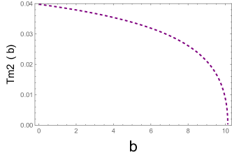
Figure 1: The temperature times $m$ depicted in dependence on $b$ for the Schwarzschild limit. Note, that the temperature is approaching zero as $b$ approaches 10.125.

As a general result, the Hawking temperature starts at the known value for $b=0$ (GR) and tends to zero for $b=\frac{81}{8}$. For the last value, there is no emission from the black hole at the event horizon, implying $T=0$ and a stable black hole, which does not evaporate. In fact, at this point the black hole ceases to exist and is a normal dark star, no emissions.

This strange behavior is linked to the negative heat capacity, which is obtained deriving $T$ with respect to $m$. Because $T$ is inverse proportional to $m$, the heat capacity will be proportional to $-1/m^{2}$. I.e., when $m$ increases, the entropy increases but the temperature decreases and vice versa.

3.1.2 Entropy, for the case $a=0$ and $l=0$

The relation between the entropy and energy is given by the thermodynamical relation (no electric charge, no angular momentum)

$$dE~{}=~{}dm = TdS~{}~{}~{},$$ (19)

where $m$ is the energy (mass) of the system (note that $c=1$).

Substituting (18) for $T$ leads to the differential equation

$$dS = \left(2\pi my_{h}^{2}\right)dm\left[\left(1-\frac{b}{3y_{h}^{2}}\right)\right]^{-1}~{}~{}~{}.$$ (20)

Inspecting (20) the $dS$ is proportional to $mdm$ and it can be integrated easily, leading to

$$S = \frac{m^{2}}{2}\left(2\pi y_{h}^{2}\right)\left[\left(1-\frac{b}{3y_{h}^{2}}\right)\right]^{-1}~{}~{}~{}.$$ (21)

Now, the factor $\left(1-\frac{b}{3y_{h}^{2}}\right)$ is in the denominator! This implies that the entropy goes to infinity toward the event horizon, while $T$ goes to zero, which is the result of the simplified approximations applied. Nevertheless, the product $TdS$ is constant and is always given by $dm=dE$, i.e., finite.

3.2 The Kerr case for $l=0$

The metric, in terms of the radial variable $y$, is given in (15). In order to obtain the position of the event horizon, the equation (16) has to be resolved. The corresponding figure is depicted in Fig. 2, where the dependence in terms of $b$ and $a$ is given [17]. The main observations are: For $b=\frac{81}{8}$ there is still an event horizon at $a=0$. However, as soon as $a>0$ there is no event horizon anymore. Also, for a given $b$, increasing $a$ leads at some point on to the disappearance of the event horizon. The curve at the bottom of Fig. 2 traces the projection of the event horizon, in dependence on $a$ and $b$.

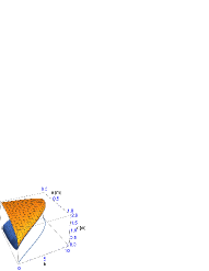
Figure 2: The position of the event horizon $r_{h}=my_{h}$, as a function on the dark energy parameter $b$ and the rotational paraneter $a$ [17]. The lower sheet in the figure corresponds to inner event horizons, also a solution of (16).

The Hawking temperature is calculated in the same manner as explained in the last section, save that now there is an additional dependence on $a$.

For the temperature we obtain

$$T = \frac{\kappa}{2\pi}~{}=~{}\frac{1}{2\pi my_{h}^{2}}\left(1-\frac{a^{2}{\rm cos}^{2}(\theta)}{y_{h}}-\frac{b}{3y_{h}^{2}}\right)\left(1+\frac{a^{2}{\rm cos}^{2}(\theta)}{y_{h}}\right)~{}~{}~{}.$$ (22)

Also, here we set $y=y_{h}$, but as mentioned, the same formula is valid for any position $y$. In Fig. 3 the temperature times the mass $m$ is depicted in dependence on $a$ and $b$. For $a=0$ the temperature decreases continuously towards zero, as obtained in the former section.

Also interesting is plotting the temperature, times $m$, as a function in $y$ and $b$ for two different cases of $a$, namely 0 and 1. The result is given in Fig. 4. In Quantum Electrodynamics particle pairs can be created in strong electromagnetic fields, which is called the Schwinger effect [18]. With the same reason, we can assume the possibility that pair production can happen in strong gravitational fields,as shown in [10].

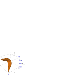
Figure 3: The dependence of the temperature, multiplies with the mass parameter $m$, on the rotational parameter $a$ of the Kerr metric and on the dark energy parameter $b$. We used $\epsilon=\frac{l}{m}=0.01$.

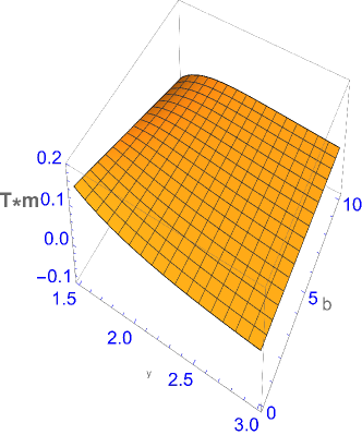
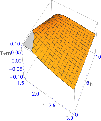
Figure 4: $T$ times $m$ is plotted versus $y$ and $b$. Note, due to the large mass ($\epsilon=\frac{l}{m}=0$), there is no effect of the minimal length.

In Fig. 5 the function $Tm$ is plotted versus $y=\frac{r}{m}$. For a non-zero value of $b$, vacuum fluctuations are simulated. The effect of them is a peak in the function $Tm$, as also obtained in [16], where the vacuum fluctuations were calculated using first principles. The fact that by our phenomenological ansatz we obtain a similar structure shows the usefulness of phenomenological approaches in getting useful insights. The left panel in Fig. 5 is for setting the minimal length equal to 0, while the right panel is for $\epsilon=\frac{l}{m}=0.01$ (see next sub-section). The change is not significant, implying that the mere presence of vacuum fluctuation creates this peak. When $b=0$ (no vaccum fluctuations), the function $Tm$ is steadily decreasing in $r$, with no peak.

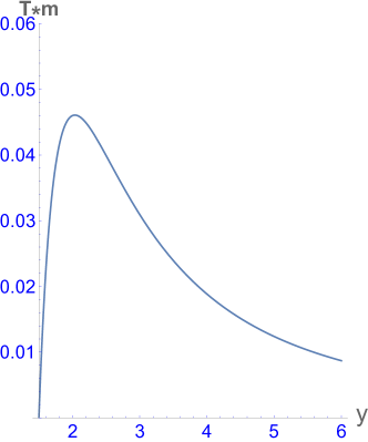
Figure 5: $T$ times $m$ is plotted versus $y$, for $b=\frac{81}{8}$. The left panel shows the result without the factor $\sigma^{2}$ and the right panel with this factor. The value $\epsilon=0.01$ was used.

For the entropy, we obtain

$$dS = \left(2\pi my_{h}^{2}\right)dm\left[\left(1-\frac{a^{2}{\rm cos}^{2}(\theta)}{y_{h}}-\frac{b}{3y_{h}^{2}}\right)\left(1+\frac{a^{2}{\rm cos}^{2}(\theta)}{y_{h}}\right)\right]^{-1}~{}~{}~{},$$ (23)

which exhibits the same behavior as in the last section. It tends to infinity toward an event horizon, but because $T$ tends to 0 at the event horizon, the product $TdS$ stays constant.

3.3 The general case: Kerr metric, with $l>0$

When $l>0$ another distinct property emerges more pronounced, namely negative temperatures. This sounds at first strange, because in classical mechanics negative temperatures are not possible. In classical physics, the temperature is related to the mean kinetic energy of particles in a gas. The temperature increases when the energy of the system increases. However, this changes in Quantum systems, when there is an upper bound to the energy [7, 19]. When energy increases, the temperature also increases, until half of the possible energy, which can be deposited is reached. From that point on, though the energy increases, the temperature becomes negative. In different words, negative temperature describes systems which are hotter than systems with a positive temperature [7, 20]. A central point is that the stability relation $\frac{\partial S}{\partial V}$ = $\frac{p}{T}>0$ is valid, where $S$ is the entropy, $V$ the volume, $p$ the pressure and $T$ the temperature. Thus, when $T$ is negative, the pressure has to be negative, too. Consequently, at negative temperature there is also a negative pressure, which can stabilize a black hole [7]. A useful reference on negative temperature and measurements in real physical systems is given in [21, 22].

In this context, we discuss the effects when a minimal length is included. The infinitesimal length squared changes to [23, 24]

$$d\omega^{2} = \sigma^{2}(r)g_{\mu\nu}dx^{\mu}dx^{\nu}~{}~{}~{},$$ (24)

with

$$\sigma^{2}(y) = \left(1-l^{2}\mid a\mid^{2}\right)~{}~{}~{}.$$ (25)

where $\mid a\mid^{2}$ is the absolute value of the acceleration. As noted by [13], the presence of an acceleration breaks covariance. The extraction of the factor $\sigma^{2}$ has to be seen as an approximation in order to include acceleration effects. Thus, the $\sigma^{2}(y)$ is a function of the acceleration. In terms of the accelerations it is given by

$$\sigma^{2}(r) = 1-l^{2}\left[\left(1-\frac{\Psi}{y^{2}}\right)\left(\overset{..}{t_{0}}\right)^{2}-\frac{y^{2}}{\Delta}\left(\overset{..}{y}\right)^{2}\right.$$ (26)

$$\left.-\left(\left(y^{2}+\alpha^{2}\right)+\frac{\alpha^{2}\Psi}{y^{2}}\right)\left(\overset{..}{\phi}\right)^{2}+\frac{2\alpha\Psi}{y^{2}}\left(\overset{..}{t_{0}}\overset{..}{\phi}\right)\right]~{}~{}~{}.$$

with

$$\Sigma = y^{2}+a^{2}\cos^{2}\theta$$ (27)

$$\Delta = y^{2}+a^{2}-\Psi$$ (28)

$$\Psi = 2y-\frac{b}{6y^{2}}$$ (29)

The accelerations $\ddot{t}$, $\ddot{y}$ and $\ddot{\phi}$ are given in [23] and will not be listed here.

Again, the Hawking temperature is given by $T=\frac{\kappa}{2\pi}$, where $\kappa$ is proportional to the derivative of $g_{00}$, as defined before. As we saw, this temperature, times the mass $m$, can be defined as a function in $y$, implying that also at space positions different to the event horizon, there exists the possibility to produce pairs of particle-antiparticles, just like the mentioned Schwinger effect [18] in Quantum Electrodynamics. Thus, when we plot the Hawking temperature as a function in $y$, we can access important information on particle pair production at any point in space. The dependence of the temperature on the position in the gravitational field was already investigated in [25]. The temperature has two terms, one proportional to $\sigma^{2}$ and the other one to the derivative of it. I.e., when $\sigma^{2}<0$, the temperature becomes negative, which is only valid if this happens for $y\geq y_{h}$. This is a more dominant effect because $\sigma^{2}$ can have singularities, even for $y\geq y_{h}$. On the right hand side of Fig. 5 the result for including $\sigma^{2}$ is shown, which is similar to [16], showing the advantage of our phenomenological path, compared to first principle approaches.

In Fig. 6 the Hawking temperature is plotted versus $y$ and $b$ for three different values of $a$ (0, 0.5 and 1). For $a=0$ we note a ridge still appearing at $y>y_{h}$ (the structure at $y<y_{h}$ can be ignored, because we do not include mass distributions), representing a singularity, which follows the position of the event horizon, starting at $y=2$ for $b=0$ and ending at $y=1.5$ for $b=\frac{81}{8}$. When increasing $a$ the end of the ridge moves to lower values of $b$ and vanishing for $a=1$, where no event horizon exists anymore.

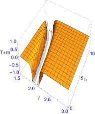
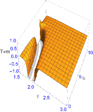
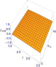
Figure 6: The Hawking temperature time $m$ as a function on $b$ and $y$. The most left figure depicts the results for $a=0$, the centered one for $a=0.5$ and the right one for $a=1$. We used $a=0$ and $\epsilon=\frac{l}{m}=0.01$, i.e., a black hole mass which is 100 times larger than the Planck mass. The structure below $y_{h}$ can be ignored, because there is mass present.

Another feature is the appearance of a singularity, where the temperature lowers to infinite negative values, for $y\geq y_{h}$. As exposed in [7], negative temperatures correspond to negative pressure, i.e. it works against the gravitational attraction and stabilizes the black hole. This was verified experimentally, simulating a black hole by a Ising-spin systems [26]. There it is shown that the Ising spin system simulates a Schwarzschild black hole, where the strength of the applied magnetic field is equivalent to the mass [26]. In pcGR this is the consequence of the presence of dark energy, acting repulsively.

In Fig. 7 the Hawking temperature times $m$ is plotted up to $b=15$, which is above the value of $\frac{81}{8}$, where the last event horizon exists for $a=0$. As can be appreciated, the temperature does not exhibit a singularity as soon as no event horizon exists, in agreement to the Fig. 6, where above a specific $a$ value, from which on no event horizon exists, the temperature also does not exhibit a singularity.

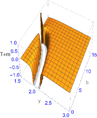
Figure 7: The Hawking temperature times $m$ as a function on $b$ and $y$, for a=0 but $b$ ranges up to 15. As can be appreciated, for $B>10.125$, when no event horizon exists, the temperature does not show a singularity. We used $a=0$ and $\epsilon=\frac{l}{m}=0.01$, i.e., a black hole mass which is 100 times larger than the Planck mass. The structure below $y_{h}$ can be ignored, because there is mass present.

One of the main take-aways is when an event horizon is present, the Temperature rises to very large negative values for $y$ near above the event horizon. Negative temperatures are hotter than positive temperatures [7] and the result implies an immediate evaporation of the black hole. All this is only valid for small masses, of few orders of the Planck mass, and disappears for large masses. The implication is that the production of small black holes, as speculated, is highly suppressed. Thus, according to our theory, black holes can only form when they are rapidly produced and with a large mass.

4 Conclusions

In this contribution we resumed the pcGR and discussed their consequences, which are i) the existence of a minimal length, ii) the appearance of a dark energy-momentum tensor on the right hand side of the Einstein equations and iii) some experimental predictions. The concept of a generalized Mach’s principle is presented, implying that a mass not only curves space-time but also modifies the vacuum structure around that mass.

We then investigated the consequences of a minimal length for the Hawking temperature and the entropy in the general case of a rotating stellar object (Kerr metric) with a minimal length present. The results presented include GR and theories which inlcude dark energy.

For massive objects, as a massive star or black hole, no effects of the minimal length are found. The situation changes significantly when the stellar object is small, like a mini-black hole. Thus, the consequences obtained here are rather valid only for very small objects, of a few orders of the Planck mass. Therefore, it may only play a role at the beginning of the universe where such objects are assumed to be produced.

At the event horizon, the Hawking temperature decreases with increasing accumulation of dark energy, described by a parameter $b$ in the theory. There is a maximum value ($\frac{81}{8}$) where the temperature reaches zero (no emission) at the event horizon and the entropy tends to infinity, however, for larger distances the temperature is again positive and shows a maximum at a finite radial distance. This singularity is a consequence of the simplified assumption of the dark energy distribution. When the minimal length is present, the metric involves a factor $\sigma^{2}$, which depends on the acceleration of a particle. This function shows a singularity at the event horizon, when $g_{00}=0$, which This produces negative values in the Hawking temperature, tracing the position of the event horizon. As soon as $b>\frac{81}{8}$, no large negative temperatures appears and the Hawking temperature has finite values. Small black holes evaporate explosively due to the appearance of a negative temperature at an event horizon. Thus, their very production is strongly suppressed. It appears that negative temperatures only appear due to the event horizon, because when no event horizon exists, the temperature remains finite. Negative temperatures also imply a negative pressure [7], which is explained in pcGR by the presence of dark energy, stabilizing the black hole. There is also the case when $T=0$, which implies that there is no radiation and the star is stable.

These findings are only valid for very small stellar objects. According to our findings, black holes have to be produced rapidly and with large masses, in order to survive.

References

- [1] P. O. Hess, W. Greiner, Int. J. Mod. Phys. E 18 (2009), 51.
- [2] P. O. Hess, M. Schäfer, W. Greiner, Peudo-Complex General Relativity, (Springer, Heidelberg, 2015).
- [3] P. O. Hess, Alternatives to Einstein’s Relativity Theory, Prog. in Part. and Nucl. Phys. 114 (2020) 103809.
- [4] P. O. Hess, AN 342 (2021),735.
- [5] Hess, publ. where light emission near the poles is predicted.
- [6] Y. Kluger, J. M. Eisenberg, B. Svetitsky, F. Cooper, E. Mottola, Physical Review Letters 67 (1991), 2427.
- [7] R. A. Norte, EPJ 145 (2024), 29001.
- [8] P. F. Kelly, R. B. Mann, Ghost properties of algebraically extended theories of gravitation, Class. and Quant. Grav. 3, 705 (1986).
- [9] N. D. Birrell, P. C. W. Davis, Quantum Fields is Curves Space, Cambridge University Press, London, (1982).
- [10] M. Visser, Phys. Rev. D 54 (1996) 5116.
- [11] R. Adler, M. Bazin, M. Schiffer, Introduction to General Ralativity, 2nd edition, (Mcgrw-Hill, New York, 1975).
- [12] E. R. Caianiello, Il Nuovo Cim. Lett. 32 (1981), 65.
- [13] A. Feoli, G. Lambiase, G. Papini, G. Scarpetta 2000, Phys. Lett. A 268 (2000), 247.
- [14] G. Caspar, I. Rodríguez, P. O. Hess, W. Greiner, Int. J. Mod. Phys. E 25 (2016), 1650027.
- [15] T. Padmanabhan, Phys. Rep. 406 (2005), 49.
- [16] M. F. Wondrak, W. D. van Suijlekom, Heino Falcke, Phys. Rev. Lett. 130 (2023), 221502.
- [17] P. O. Hess, E. López-Moreno, Universe 5 (2019), 191.
- [18] F Gelis, N Tanoi, Progr. Part. Nucl. Phys. 87 (2016), 1.
- [19] W. Greiner, L. Neise, H. Stoecker, Themrmodynamics and Statistical Mechanics, (Springer Heidelberg, 1995).
- [20] N. F. Ramsey, Phys. Rev. 103 (1956), 20.
- [21] S. Braun, Negative Absolute Temperature and the Dynamics of Quantum Phase Transitions, PhD thesis, Fakultät für Physik der Ludwig-Maximilians-Universität München, Germany (2014).
- [22] S. Braun,1, J. P. Ronzheimer, M. Schreiber, S. S. Hodgman, T. Rom,1, I. Bloch, U. Schneider, Science 339 (January 4) (2013), 52.
- [23] L. Maglahoui, P. O. Hess, AN 344 (2022), 220067.
- [24] L. Maghlaoui, P. O. Hess, AN 345 (2024), 20230151.
- [25] R. C. Tolman and P. Ehrenfest, Phys. Rev. 36 (1930), 1791.
- [26] Oppenheim J., Phys. Rev. E 68 (2003), 016108.