LOG-LIO2: A LiDAR-Inertial Odometry with Efficient Uncertainty Analysis
Kai Huang1, Junqiao Zhao∗,2,3, Jiaye Lin2,3, Zhongyang Zhu2,3, Shuangfu Song1, Chen Ye2, Tiantian Feng11Kai Huang, Shuangfu Song and Tiantian Feng are with the School of Surveying and Geo-Informatics, Tongji University, Shanghai, China
(e-mail: huangkai@tongji.edu.cn; songshuangfu@tongji.edu.cn; fengtiantian@tongji.edu.cn).2Junqiao Zhao, Jiaye Lin, Zhongyang Zhu and Chen Ye are with Department of Computer Science and Technology, School of Electronics and Information Engineering, Tongji University, Shanghai, China, and the MOE Key Lab of Embedded System and Service Computing, Tongji University, Shanghai, China
(e-mail: zhaojunqiao@tongji.edu.cn; 2233057@tongji.edu.cn; 2310920@tongji.edu.cn; yechen@tongji.edu.cn).3Institute of Intelligent Vehicles, Tongji University, Shanghai, China.Digital Object Identifier (DOI): see top of this page.
Abstract
Uncertainty in LiDAR measurements, stemming from factors such as range sensing,
is crucial for LIO (LiDAR-Inertial Odometry) systems as it affects the accurate weighting in the loss function.
While recent LIO systems address uncertainty related to range sensing, the impact of incident angle on uncertainty is often overlooked by the community.
Moreover, the existing uncertainty propagation methods suffer from computational inefficiency.
This paper proposes a comprehensive point uncertainty model that accounts for both the uncertainties from LiDAR measurements and surface characteristics, along with an efficient local uncertainty analytical method for LiDAR-based state estimation problem.
We employ a projection operator that separates the uncertainty into the ray direction and its orthogonal plane.
Then, we derive incremental Jacobian matrices of eigenvalues and eigenvectors w.r.t. points, which enables a fast approximation of uncertainty propagation.
This approach eliminates the requirement for redundant traversal of points, significantly reducing the time complexity of uncertainty propagation from to when a new point is added.
Simulations and experiments on public datasets are conducted to validate the accuracy and efficiency of our formulations.
The proposed methods have been integrated into a LIO system, which is available at https://github.com/tiev-tongji/LOG-LIO2.
I INTRODUCTION
Uncertainty stemming from sensor limitations, measurement noises, and unpredictable physical environments plays a crucial role in robotic state estimation, as it affects the accurate weighting of distance metrics in the loss function [1].
One common approach is to model the measurement uncertainty using zero-mean Gaussian noise with respect to point coordinates and integrates these noises into the state estimation.
However, such uncertainty modeling of LiDAR measurements is not precise.
To address this issue, [2] develops a point uncertainty model that incorporates both range and bearing, while [3] further includes the surface roughness.
These uncertainties are then propagated to the geometric elements such as planes, which are utilized for weighting the point-to-element distance in scan-to-map registration, thereby enhancing the accuracy and reliability of the system [2, 4, 5].
However, range uncertainty is also influenced by the incident angle [6, 7], a factor often overlooked by existing studies.
Additionally, continuous propagation of uncertainty from numerous points, which exhibits linear time complexity , can be computationally expensive, particularly for dense point cloud and real-time applications.
Therefore, an efficient uncertainty propagation method is highly desirable.
In this paper, we present a comprehensive point uncertainty model that incorporates all relevant factors affecting LiDAR measurements, including range, bearing, incident angle, and surface roughness.
This model leverages the projection operator [7] to separate the uncertainty into the ray direction and its orthogonal plane. And we demonstrate the consistency of our method with existing methods [2, 4, 5].
To accelerate the propagation of uncertainty from points to the geometric elements,
we derive the incremental Jacobian matrices for eigenvalues and eigenvectors corresponding to specified points from Welford’s formulation [8].
The parametric uncertainty of the geometric elements is then updated incrementally by fast approximations.
We validate the efficiency and accuracy of the fast uncertainty approximation through simulation experiments.
Subsequently, we integrate these methods into a LIO system named LOG-LIO2.
By comparing the performance of LOG-LIO2 with state-of-the-art LIO systems, i.e. VoxelMap [5], LOG-LIO [9] and FastLIO2 [10], we demonstrate the performance improvement achieved by the proposed techniques.
The main contributions of this work are as follows:
•
A comprehensive point uncertainty model with a fast calculation method,
incorporating the uncertainty of range and bearing measurements from LiDAR,
as well as incident angle and roughness concerning the target surface.
•
A fast approximation of uncertainty propagation from points to eigenvalues and eigenvectors by leveraging the incremental Jacobian matrices,
reducing the time complexity from to by eliminating the need for repetitive calculations when a new point is added.
•
We demonstrate the efficiency and accuracy of our methods from both simulation and public datasets.
The methods proposed in this paper are incorporated into a LIO system which is available at https://github.com/tiev-tongji/LOG-LIO2.
II RELATED WORKS
The integration of IMU has significantly improved the practical robustness of LIO systems [11].
However, a critical limitation persists in these systems: the uncertainty of each point is treated homogeneously, neglecting potential spatial and environmental variations that can significantly impact accuracy.
[2] investigates the physical measuring principles of LiDAR and derives the uncertainty model for each laser beam encompassing range and bearing uncertainties.
Specifically, the bearing uncertainty is modeled as a perturbation [12] in the tangent plane of the ray.
However, the calculation of perturbation requires the construction of two bases in the tangent plane, leading to increased computational cost.
[4] introduces a novel adaptive voxelization method that iteratively divides voxels until the point distribution matches the line or plane geometry.
The paper derives the Jacobian and Hessian matrices of eigenvalues and eigenvectors w.r.t. the points within the voxel, leveraging these matrices for LiDAR bundle adjustment.
Building on these prior works, VoxelMap [5] integrates the point uncertainty model and adaptive voxelization technique into a LiDAR-based odometry system.
The uncertainty associated with each point is then propagated to the plane parameters to weight the point-to-plane distance in the state estimation.
However, the traversing of all points during propagation reduces the real-time performance of the system.
In addition to inherent laser range and bearing uncertainties, the geometrical properties of the target surface also contribute significantly to observed point uncertainty.
[6] and [7] analyze the geometrical relationship between the laser beam and the surface normal, incorporating the uncertainty arising from the incident angle into the ray direction.
While they obtain a closed-form approximation of this uncertainty, it is overlooked by the SLAM community.
Distinct from prior works, [3] introduces a principled uncertainty model for LiDAR scan-to-map registration.
This model incorporates the roughness of the measured uneven planes, thereby enhancing robustness but also introducing complexity in estimation.
Having the above, our focus is on developing a comprehensive point uncertainty model and deriving efficient uncertainty propagation methods, aiming to strike a balance between accuracy and computational efficiency.
III PRELIMINARY
In this paper, we assume the transformation between LiDAR and IMU is calibrated in advance.
We consider as the center of point cloud .
The sum of the outer products of all points deviating from is S,
which is normalized to A, i.e. the covariance,
(1)
where the superscript indicates a specified cloud with points.
For the symmetric matrix A, eigenvalue decomposition is performed as follows:
(2)
where is the eigenvector corresponding to the eigenvalue with .
IV Point Uncertainty Model
Modeling the point uncertainty derived from the range and bearing measurements as [2, 4, 5] is natural since the coordinate is obtained from the relative position w.r.t. the LiDAR.
However, the geometric properties of the target surface, i.e. incident angle and roughness, also contribute to the uncertainty of the LiDAR measurements [3, 6, 7].
Our uncertainty model takes into account both the properties of the sensor itself and the observed geometry.
We assume the uncertainty follows a Gaussian distribution.
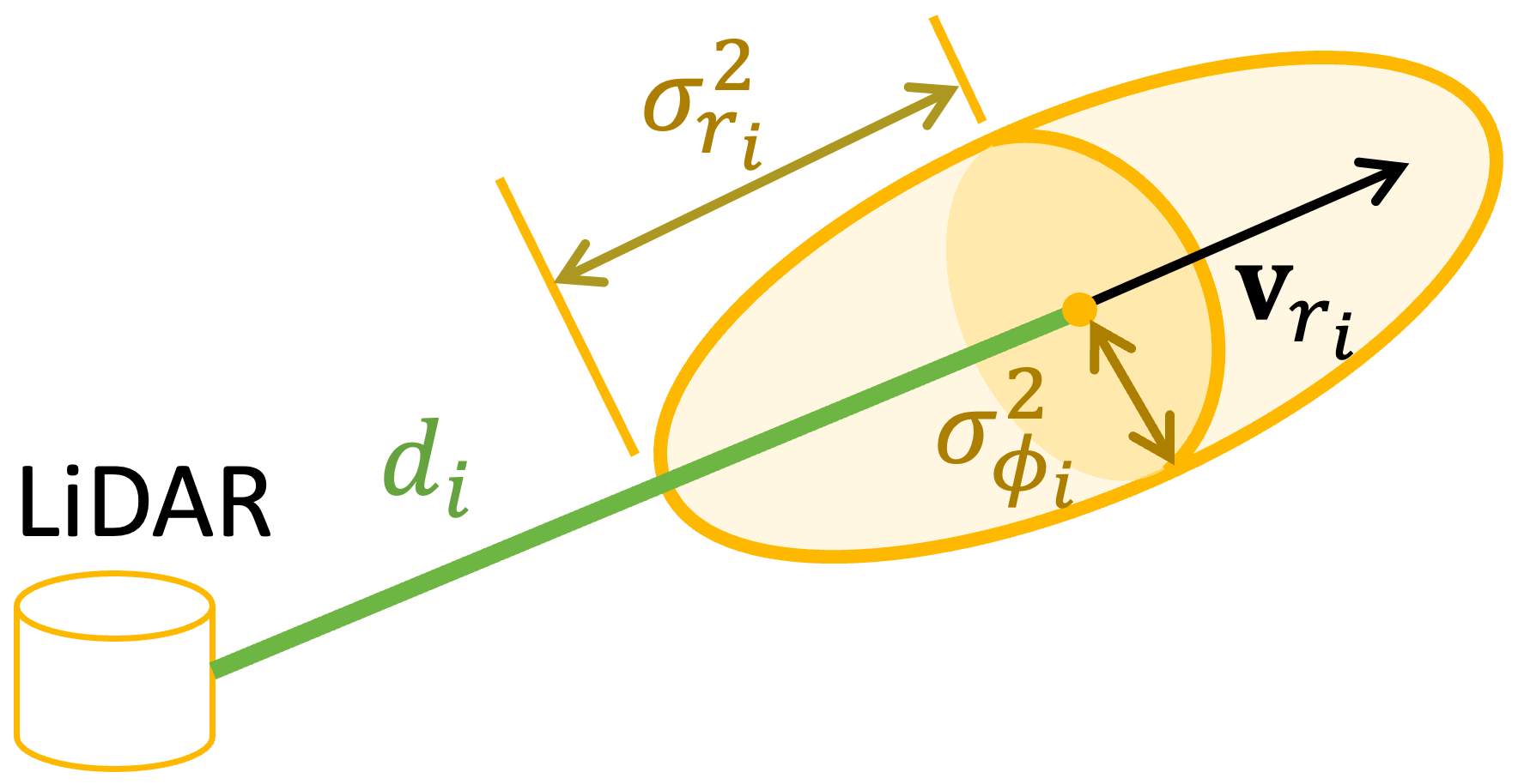
Inspired by [7] and as shown in Figure 1(a), we denote the magnitude of uncertainty along the ray as
while the magnitude of uncertainty in the direction orthogonal to is denoted as .
Note that the orientation of is not specified in order to simplify the calculations, as further explained in Section IV-B.
(a)point uncertainty model
(b)incident angle and roughness
Figure 1: Illustration of geometric relationship for the point uncertainty model.
IV-AUncertainty Factors
IV-A1 Range and bearing
Similar to [2, 5], we assume that the magnitude of the range and bearing uncertainty to each laser beam are both constant factors,
and , respectively.
In a 3D space, the extends in the , while is isotropic in the orthogonal plane of the .
IV-A2 Incident Angle
As illustrated in Figure 1(b), the incident angle between the laser beam and the surface normal, plays a pivotal role in the range sensing [7].
As increases from 0 to , the range uncertainty also rises.
We model the uncertainty caused by the incident angle along the ray direction,
(3)
where is the distance from to the LiDAR.
IV-A3 Roughness
We account for the impact of surface roughness on the point in a simpler and faster manner compared to [3].
To achieve this, we estimate the normal of the target surface by analyzing two different neighborhood scales.
As shown in Figure 1(b), the angle formed between these two normals serves as a metric for quantifying the uncertainty introduced by the roughness:
(4)
where is a preset value,
and are normals estimated under different neighborhood scales.
IV-BFast Uncertainty Calculation
Assuming the roughness is isotropic in 3D space,
we integrate the aforementioned three factors to compute the covariance of a point as follows:
(5)
where , , and is the unit vector in ray direction.
The projection operator is employed to isotropically project the magnitude of the bearing uncertainty onto the 2D plane that is orthogonal to in 3D space [7].
Note that considering only the uncertainty of range and bearing, our method aligns with [2, 4, 5], which is proved in Appendix A-A.
And we present a more comprehensive point uncertainty model accompanied by an efficient method that offers greater geometric interpretability.
V LUFA: Local Uncertainty Fast Approximation
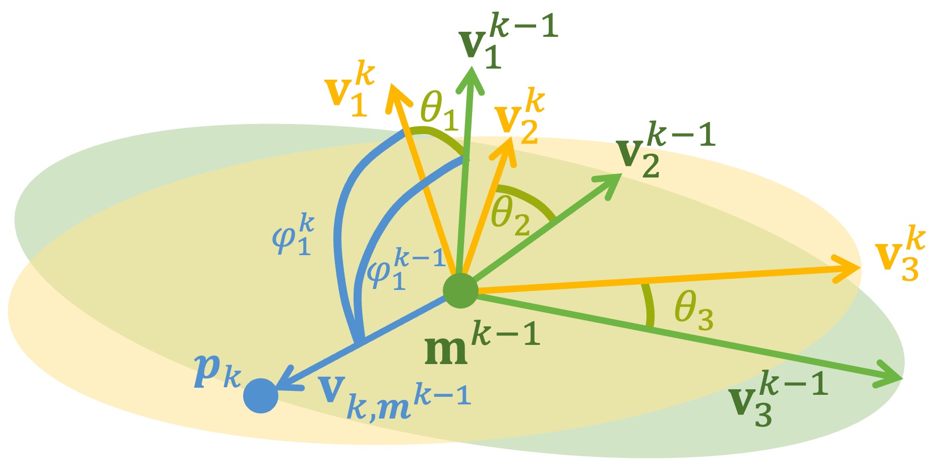
As outlined in BALM [4], given a set of points ,
computing the center, covariance, and propagation of point uncertainty to the eigenvalues and eigenvectors,
necessitates traversing all points in resulting in time complexity.
This can hinder real-time performance.
To relieve this computation burden, we propose an incremental update approach to compute these statistics, achieving time complexity when a new point is added.
This enhancement ensures real-time performance, making it more suitable for applications like SLAM.
V-AIncremental Center and Covariance
Using Welford’s formula [8], we incrementally update the center m and covariance S of as follows:
(6)
(7)
where and are updated from and , is the newly added point.
Define and combine (1),
the normalized covariance can be updated incrementally as follows:
(8)
The updated covariance can be decomposed into two terms:
the first term scales the covariance of the existing point cloud,
while the second term captures the incremental contribution of the newly added point .
V-BIncremental Jacobian of Eigenvalues
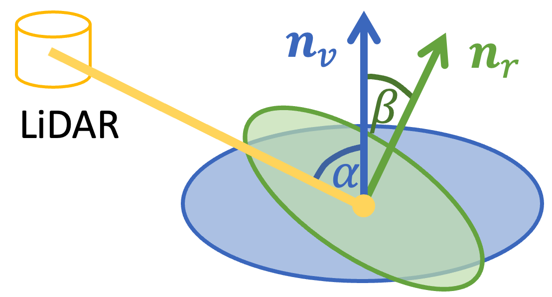
The partial derivative of w.r.t. the point is given by:
(9)
where is the distance between and , is the angle between and .
Define , then and are angles from the direction of to and , respectively.
The proof of (9) is provided in Appendix A-B.
Figure 2:
Illustration of geometric relationship for the local frame.
Figure 2 visually depicts the geometric relationships involved in (9).
To clarify the geometric meaning, let’s consider , the normal of a plane, as an example, which determines the direction for calculating the point-to-plane distance.
Suppose that with a sufficient large number of points sampled from the plane and lies on it, then, and .
Consequently, the second term of is approximately equal to 0.
Furthermore, the second term (incremental terms) of (9) are identical for the first points.
This characteristic allows for their efficient computation without the need to traverse .
We take the magnitude of the second term of (9) to determine the update form of the Jacobian matrix of the eigenvalues.
If the magnitude is smaller than a threshold, we approximately update the Jacobian as follows:
(10)
Otherwise, the Jacobian is updated in the manner of BALM [4] :
(11)
Considering that is independent of , the Jacobian matrix of eigenvalues w.r.t. can be simplified as,
According to BALM [4], the Jacobian matrix of the eigenvectors w.r.t. can be represented as:
.
For the element in -th row and -th column in :
(13)
And (13) can be further simplified as
,
where the subscripts and are elements of .
Since diagonal elements in is equal to 0,
The rest of this section only specify the form of the off-diagonal elements.
Analogous to the Jacobian matrix of the eigenvalues, for , the matrix above can be incrementally updated,
which is also divided into scale and increment parts:
(14)
where and are angles from to and , respectively.
We specify the form of and prove (14) in Appendix A-C.
With the assumption that a sufficient large number of points already sampled from the surface, the second term of (14) is approximately equal to 0.
Take , i.e. normal , of the surface as an example,
the partial derivative of the updated w.r.t. can be approximately updated as follows:
(15)
where we omit some of the subscripts to simplify the representation.
Considering that is independent of , the matrix w.r.t. can be simplified as,
(16)
We prove (16) in Appendix A-C and define to simplify the representation.
V-DIncremental Update of Covariance
Using the above incremental Jacobian matrix of the eigenvalues (10) and the eigenvectors (15), their covariance can be updated in an approximate form.
We simply divide the covariance of the eigenvalues corresponding to specified points into scale and increment parts as follows:
(17)
Similarly, the covariance of the eigenvector can be updated as follows:
(18)
where we omit some of the subscripts to simplify the representation.
This fast approximation method for covariance can be seamlessly integrated with other statistical metrics sharing similar scaling properties.
Derived from (6), we get easily.
Furthermore, can be incrementally updated as,
(19)
Combining (18) and (19), the covariance of the normal and center can be fast approximated as follows:
(20)
In contrast to methods like VoxelMap [5], (20) offers a significant computational advantage by achieving a constant time complexity of .
This translates to faster execution, making it well-suited for real-time applications.
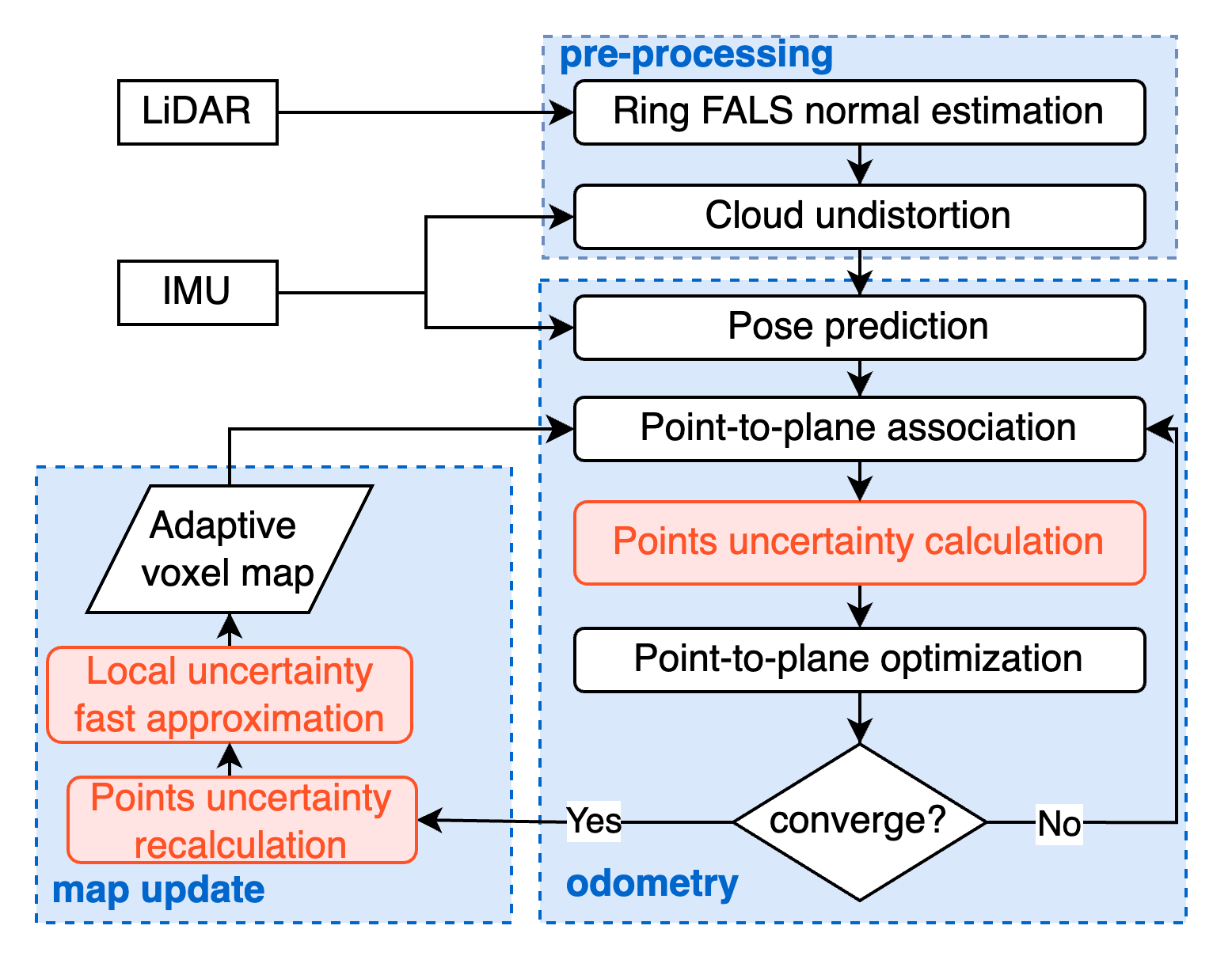
VI Integration with LIO
In this section, we integrate the proposed point uncertainty model along with the uncertainty fast approximation methods into our prior work [9], namely LOG-LIO2.
The system state is as follows:
(21)
where, and are the orientation, position and velocity of IMU in the world frame, and are gyroscope and accelerometer bias respectively, is the known gravity vector in the world frame.
Figure 3: System overview of LOG-LIO2 with enhancements marked in red.
The overall system structure is depicted in Figure 3.
It comprises three modules: pre-processing, odometry and map update.
We employ adaptive voxelization from VoxelMap [5] for map management, leveraging its efficient data association and incorporating the computation of within-voxel covariance.
VI-APre-processing
For a point within the new input scan, we first estimate its normal using Ring FALS [9].
Subsequently, point cloud undistortion is performed to compensate for LiDAR motion based on IMU measurements [11].
VI-BOdometry
By incorporating the IMU measurements from the previous frame as a prediction for the current frame, we transform each point into the world frame.
Then, we perform point-to-plane association: each point is assigned to the voxel it resides in if the points within that voxel satisfy planar geometry (indicated by the minimum eigenvalue below a threshold).
We denote as the eigenvector corresponding to the minimum eigenvalue of a given voxel.
Notably, differs from in that it incorporates geometric information from all map points within the voxel, making it more suitable for the incident angle calculation (3),
whereas focuses on the local geometry of individual points in the scan.
Both and contribute to roughness estimation (4).
Point uncertainty is then calculated (see Section IV) and used to weight point-to-plane distance:
(22)
where is the center corresponding to the associated voxel.
We denote the propagated state and covariance by and respectively.
By incorporating the prior distribution and stacking all the point-to-plane associations, we obtain the maximum a-posterior estimate (MAP) as follows [11]:
(23)
where computes the difference between and in the local tangent space of ,
is the error of the -th iterate update at time , is the Jacobian matrix w.r.t. .
The point-to-plane distance is weighted by , which incorporates point, center, and normal uncertainties.
We employ iEKF [11] to optimize the system state.
VI-CMap update
After optimization, each point is assigned to the corresponding voxel with the updated state.
A crucial aspect of this module lies in propagating the uncertainty from the scan points to the voxel center, as well as its eigenvalues and eigenvectors.
The uncertainty of points is first recalculated based on the updated state.
Apart from increment magnitude checks (see Section V),
we employ LUFA considering two additional factors:
VI-C1 Map stability
To strike a balance between initial map instability and computational efficiency,
we employ LUFA after points within a voxel exceeds a predefined threshold .
VI-C2 Error accumulation
The fast approximation introduces small errors with each iteration.
To alleviate the accumulation of these errors, we limit the continuous application of LUFA to a maximum of iterations.
Beyond the above conditions, the rigorous update forms (11) and (13) are employed.
Additionally, once the point count reaches , we fix the voxel update using rigorous forms to ensure the accuracy of the local geometric information.
This adaptive strategy effectively balances stability and efficiency during map updates.
VII EXPERIMENTAL RESULTS
VII-AExperimental Settings
The experiment focuses on the following two research questions:
1) Can LUFA approximate the uncertainty computed in rigorous form?
2) Can LOG-LIO2 improve accuracy and efficiency by incorporating our point uncertainty model and LUFA?
We first validate LUFA in a simulation environment and then further test the performance of LOG-LIO2 on real-world datasets.
Our workstation runs with Ubuntu 18.04, equipped with an Intel Core Xeon(R) Gold 6248R 3.00GHz processor and 32GB RAM.
VII-BLUFA Experiments
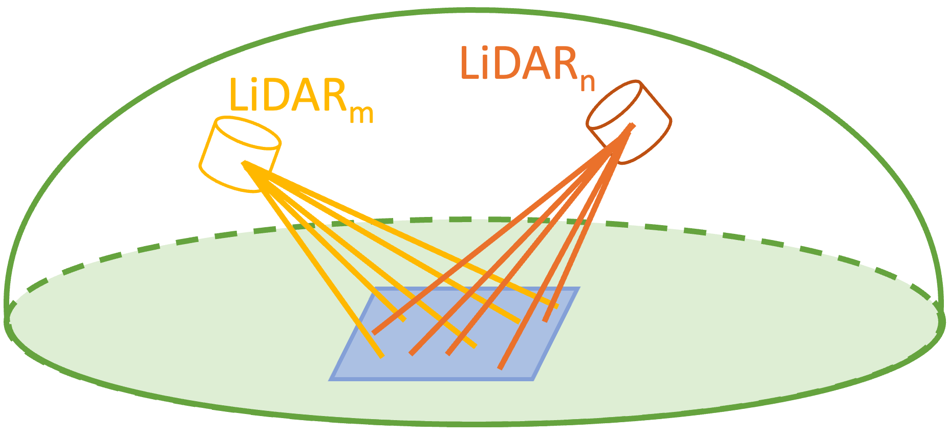
Figure 4: Illustration of the simulation environment.
To assess the accuracy and efficiency of LUFA, we benchmark it against BALM [4].
Figure 4 illustrates the validation environment, simulating a plane with 20 LiDARs, each LiDAR captures 50 points on the plane.
All LiDARs are positioned on the same side of the plane and remain within a 100m radius of its center.
The center and normal of the plane, the poses of the LiDARs, and the coordinates of the sampled points on the plane are all randomly generated.
To mimic real-world scenarios, we corrupt all these parameters with Gaussian noise, accounting for factors such as the plane’s unevenness, inaccuracies in the LiDAR poses, and measurement errors.
The point uncertainty is calculated as detailed in Section IV.
We set to define when LUFA is triggered.
VII-B1 Accuracy
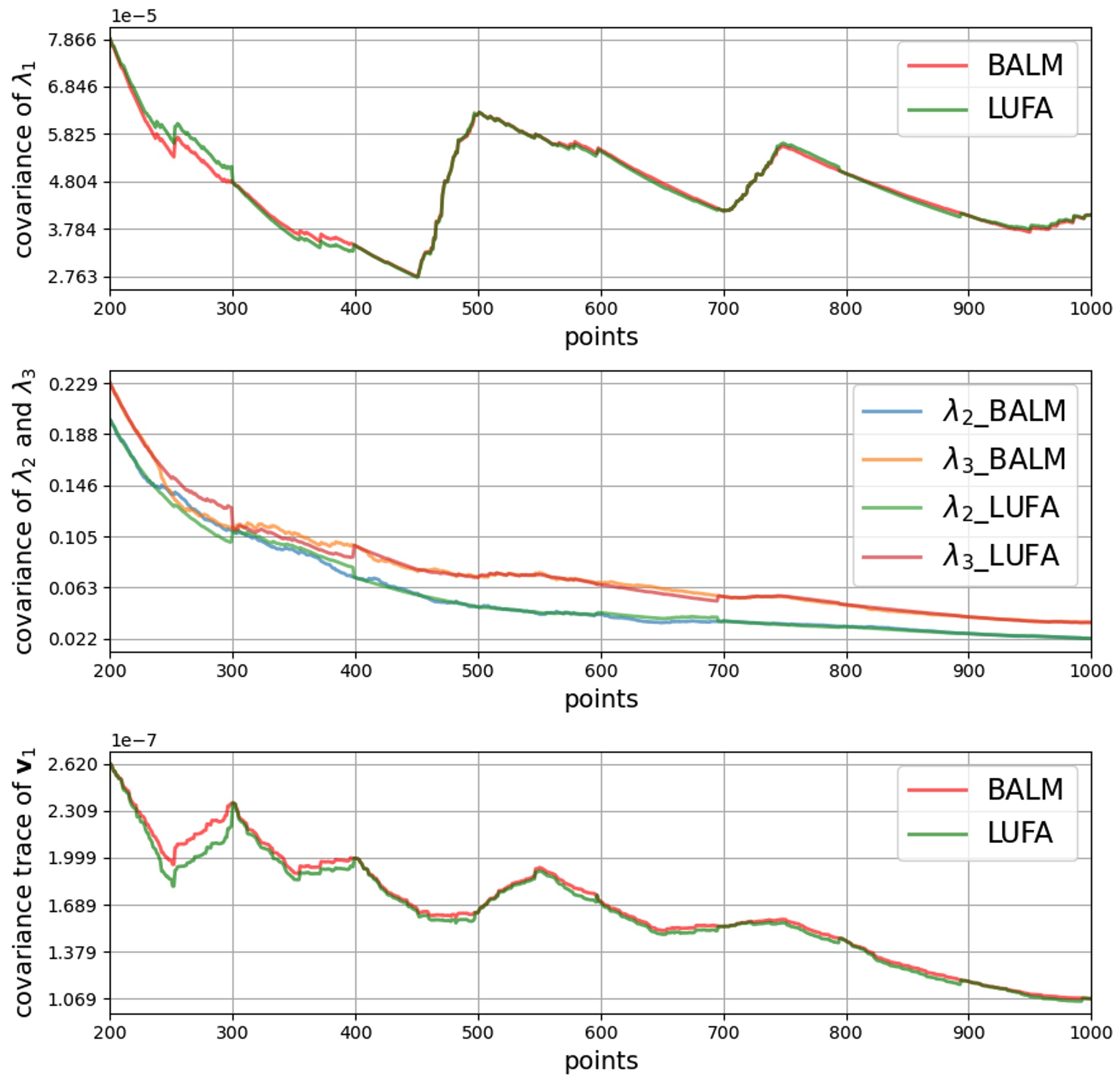
Figure 5 illustrates the covariance of the and the covariance trace of computed by LUFA and BALM.
As the covariance of the eigenvectors involves matrices, we compare the trace of the covariance matrices in our experiments, which provides a measure of the overall magnitude of the covariance.
The results indicate that the covariance computed by LUFA is close to that of BALM.
This closeness in covariance values demonstrates the effectiveness of LUFA in approximating the uncertainty propagation while maintaining a reasonable level of accuracy.
Figure 5: Comparison of covariance calculated by LUFA and BALM.
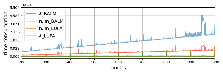
Figure 6: Time consumption for computing the covariance.
, represent the covariance of the normal and the center.
VII-B2 Efficiency
We further plot the processing time w.r.t the number of points for better evaluation in Figure 6.
As expected, BALM exhibits linear time complexity , resulting in processing time increases proportionally with the number of points.
In contrast, the processing time of LUFA remains nearly constant, adhering to time complexity.
The observed peaks in LUFA’s processing time occur at intervals of 100 points, which stems from our imposed limitation on the maximum number of consecutive LUFA executions.
Utilizing the incremental center (6) and covariance (7) ensures that even at peak processing times, LUFA remains computationally more efficient than BALM.
By comparing the results obtained using LUFA with those from BALM, we demonstrate that LUFA achieves comparable accuracy while significantly improving computational efficiency.
VII-CLIO Experiments
To evaluate the efficacy of LOG-LIO2 in real-world scenarios, we employ the M2DGR dataset[13].
This dataset collects data on a ground platform equipped with Velodyne-32 LiDAR and presents significant challenges for our previous method, LOG-LIO.
To isolate the impact of specific components within LOG-LIO2, we introduce LOG2-i, which solely leverages our point uncertainty model (Section IV) for ablation studies.
We compare the performance of LOG-LIO2 against two leading LIO methods: FAST-LIO2 [11] and PV-LIO111https://github.com/HViktorTsoi/PV-LIO.
PV-LIO is the reimplementation of VoxelMap [5] integrating IMU, showing promising results in practice.
To ensure a fair comparison, LOG-LIO2, LOG2-i and PV-LIO are executed on all dataset sequences using identical parameters: a maximum voxel size of 1.6m, and a maximum octree layer of 3, resulting in a minimum voxel size of 0.2m.
FAST-LIO2 and LOG-LIO are run with a map resolution of 0.4m.
Additionally, we set and to 200 and 1000 respectively, defining the thresholds for when LUFA is triggered and when it is no longer necessary.
Due to the instability in the RTK signal, the first and last 100 seconds of sequences street07 and street10 are excluded from the evaluation.
Noted that all the LIO systems above perform scan-to-map registration by minimizing point-to-plane distances and loop closure was disabled for all experiments.
VII-C1 Accuracy Evaluation
Table I reports the root-mean-square-error (RMSE) of absolute trajectory error (ATE).
Obviously, LOG-LIO2 and LOG2-i stand out as the most accurate LIO systems, exhibiting comparable performance, with LOG-LIO and PV-LIO following behind.
The advantage of LOG-LIO2, LOG2-i, and PV-LIO stem from a combination of an adaptive voxel map and uncertainty-weighted point-to-plane distance for scan-to-map registration.
This approach offers a more accurate geometric representation, leading to minimal registration errors.
Conversely, LOG-LIO and FAST-LIO2 depend on a fixed-scale tree structure for map management and implement noise-weighted point-to-plane distance.
Notably, LOG-LIO distinguishes itself from FAST-LIO2 by incrementally maintaining normal and point distribution within map nodes, thereby enabling the capture of geometric complexities.
TABLE I: The Translation RMSE(m) Results of Pose Estimation Comparison on the M2DGR Dataset
LOG-LIO2
LOG2-i
LOG-LIO
PV-LIO
FAST-LIO2
walk_01
0.131
0.132
0.117
0.135
0.112
door_01
0.264
0.262
0.266
0.262
0.271
door_02
0.197
0.197
0.196
0.194
0.200
street_01
0.343
0.303
0.291
0.439
0.272
street_02
2.625
2.541
3.252
3.540
2.754
street_03
0.104
0.104
0.092
0.093
0.106
street_04
1.032
1.079
0.697
1.081
0.552
street_05
0.426
0.370
0.306
0.543
0.377
street_06
0.355
0.338
0.355
0.494
0.434
street_07
0.358
0.339
0.422
0.651
3.512
street_08
0.166
0.156
0.140
0.138
0.170
street_09
1.822
1.861
2.380
1.678
3.648
street_10
0.314
0.369
0.349
0.464
0.956
mean
0.626
0.619
0.682
0.747
1.028
•
The best and second-best results are bolded and underlined respectively.
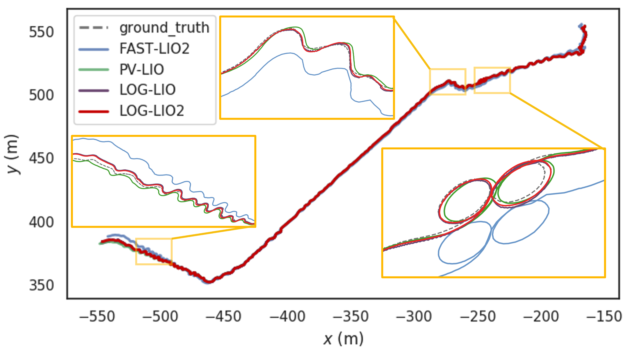
Figure 7: Localization estimates in sequence street_07 of the M2DGR dataset.
LOG2-i and LOG-LIO2 outperform PV-LIO in a majority of the sequences, benefiting from our comprehensive point uncertainty model.
PV-LIO’s model suffers from limitations: constant uncertainty in the ray direction, proportionality to range in the orthogonal plane (see (26)), and neglecting surface geometry.
In contrast, our model incorporates incident angle and surface roughness, leading to a more precise environmental representation.
This advantage is pronounced in vast outdoor environments like the street sequence.
Meanwhile, in small indoor spaces like the door sequence, all systems achieve comparable performance due to inherently lower point uncertainty and the presence of well-defined structural planes.
Figure 7 compares the trajectories in the street_07 sequence, further highlighting the performance difference.
VII-C2 Efficiency Evaluation
The processing time of LOG-LIO2, LOG2-i, and PV-LIO for the street sequence is detailed in Table II,
providing insights into both map update and runtime behavior across various thread configurations.
Note that Ring FALS introduces an additional 6ms overhead within the pre-processing module of LOG-LIO2 and LOG2-i.
Despite this overhead, comparing the average time consumption with 4 threads, LOG2-i exhibits a slightly shorter duration than PV-LIO,
mainly benefiting from the fast uncertainty calculation (Equation (IV-B)), increment center and covariance (V-A).
LOG-LIO2 stands out for its processing efficiency due to the incorporation of LUFA.
LUFA significantly accelerates map updates, leading to shorter overall processing times compared to LOG2-i and PV-LIO.
The map update module of LOG-LIO2 executes in nearly half the time of PV-LIO with a single thread and two-thirds the time with four threads.
TABLE II: The Average Time Consumption(ms) of street Sequence in The Experiments
LOG-LIO2
LOG2-i
PV-LIO
thread(s)
1
4
1
4
1
4
map update
19.13
9.29
28.67
11.92
37.98
14.56
total
59.20
50.77
68.68
52.83
80.27
59.47
VIII CONCLUSION
This paper presents a comprehensive point uncertainty model alongside a fast calculation method utilizing the projection operator.
This model incorporates not only the range and bearing uncertainty of LiDAR but also the uncertainty arising from incident angle and surface roughness.
Furthermore, we derive the incremental Jacobian matrices of the eigenvalues and eigenvectors, enabling the application of the local uncertainty fast approximation (LUFA).
The accuracy and efficiency of our formulations are first demonstrated through simulation experiments, benchmarking against the rigorous form derived by BALM.
Subsequently, we integrate all aforementioned methods into the LIO system LOG-LIO2.
Ablation experiments conducted on a public dataset validate the accuracy and efficiency of LOG-LIO2 compared to state-of-the-art LIO systems.
Appendix A
A-AConsistency of Projection Operator with Perturbation
In [2, 4, 5], the point uncertainty model considering range and bearing is derived from the perturbation of the true range and true bearing as below:
(24)
where and is range and bearing measurements respectively,
-operation encapsulated in [12],
and are range and bearing noise, respectively.
The Jacobian matrix of w.r.t. and can be further obtained as
,
where denotes the skew-symmetric matrix mapping the cross product,
and is the orthogonal basis of the tangent plane at .
Then the covariance of the point leads to:
(25)
Despite constructing arbitrarily in the tangent plane of is feasible, this approach incurs a computational cost.
We show that utilization of the projection operator simplifies the computation while maintaining consistency:
(26)
Therefore, by eliminating the need for constructing , our approach results in a more efficient method.
A-BProof of The Incremental Jacobian of Eigenvalue
Similar to BALM [4], in this section, are viewed as constant.
(8) multiplied by on the left and on the right, and combine with (2) gives:
(27)
Then the partial derivative of the updated eigenvalue w.r.t. gives:
(28)
With the value of in the last update, only the second term of the above equation needs to be solved.
where and are angles from the direction of to and , respectively.
Substituting (35), (36) and (37) into (34) yields:
(38)
It should be noted that and are scalar.
For , which is independent of , (34) degenerates into:
(39)
References
[1]
S. Thrun, “Probabilistic robotics,” Communications of the ACM, vol. 45, no. 3, pp. 52–57, 2002.
[2]
C. Yuan, X. Liu, X. Hong, and F. Zhang, “Pixel-level extrinsic self calibration of high resolution lidar and camera in targetless environments,” IEEE Robotics and Automation Letters, vol. 6, no. 4, pp. 7517–7524, 2021.
[3]
B. Jiang and S. Shen, “A lidar-inertial odometry with principled uncertainty modeling,” in 2022 IEEE/RSJ International Conference on Intelligent Robots and Systems (IROS). IEEE, 2022, pp. 13 292–13 299.
[4]
Z. Liu and F. Zhang, “Balm: Bundle adjustment for lidar mapping,” IEEE Robotics and Automation Letters, vol. 6, no. 2, pp. 3184–3191, 2021.
[5]
C. Yuan, W. Xu, X. Liu, X. Hong, and F. Zhang, “Efficient and probabilistic adaptive voxel mapping for accurate online lidar odometry,” IEEE Robotics and Automation Letters, vol. 7, no. 3, pp. 8518–8525, 2022.
[6]
T. Tasdizen and R. Whitaker, “Cramer-rao bounds for nonparametric surface reconstruction from range data,” in Fourth International Conference on 3-D Digital Imaging and Modeling, 2003. 3DIM 2003. Proceedings. IEEE, 2003, pp. 70–77.
[7]
K.-H. Bae, D. Belton, and D. D. Lichti, “A closed-form expression of the positional uncertainty for 3d point clouds,” IEEE transactions on pattern analysis and machine intelligence, vol. 31, no. 4, pp. 577–590, 2008.
[8]
B. Welford, “Note on a method for calculating corrected sums of squares and products,” Technometrics, vol. 4, no. 3, pp. 419–420, 1962.
[9]
K. Huang, J. Zhao, Z. Zhu, C. Ye, and T. Feng, “Log-lio: A lidar-inertial odometry with efficient local geometric information estimation,” IEEE Robotics and Automation Letters, vol. 9, no. 1, pp. 459–466, 2023.
[10]
C. Bai, T. Xiao, Y. Chen, H. Wang, F. Zhang, and X. Gao, “Faster-lio: Lightweight tightly coupled lidar-inertial odometry using parallel sparse incremental voxels,” IEEE Robotics and Automation Letters, vol. 7, no. 2, pp. 4861–4868, 2022.
[11]
W. Xu, Y. Cai, D. He, J. Lin, and F. Zhang, “Fast-lio2: Fast direct lidar-inertial odometry,” IEEE Transactions on Robotics, vol. 38, no. 4, pp. 2053–2073, 2022.
[12]
D. He, W. Xu, and F. Zhang, “Kalman filters on differentiable manifolds,” arXiv preprint arXiv:2102.03804, 2021.
[13]
J. Yin, A. Li, T. Li, W. Yu, and D. Zou, “M2dgr: A multi-sensor and multi-scenario slam dataset for ground robots,” IEEE Robotics and Automation Letters, vol. 7, no. 2, pp. 2266–2273, 2021.