Privacy-Enhanced Database Synthesis for Benchmark Publishing
Abstract.
Benchmarking is crucial for evaluating a DBMS, yet existing benchmarks often fail to reflect the varied nature of user workloads. As a result, there is increasing momentum toward creating databases that incorporate real-world user data to more accurately mirror business environments. However, privacy concerns deter users from directly sharing their data, underscoring the importance of creating synthesized databases for benchmarking that also prioritize privacy protection. Differential privacy has become a key method for safeguarding privacy when sharing data, but the focus has largely been on minimizing errors in aggregate queries or classification tasks, with less attention given to benchmarking factors like runtime performance. This paper delves into the creation of privacy-preserving databases specifically for benchmarking, aiming to produce a differentially private database whose query performance closely resembles that of the original data. Introducing PrivBench, an innovative synthesis framework, we support the generation of high-quality data that maintains privacy. PrivBench uses sum-product networks (SPNs) to partition and sample data, enhancing data representation while securing privacy. The framework allows users to adjust the detail of SPN partitions and privacy settings, crucial for customizing privacy levels. We validate our approach, which uses the Laplace and exponential mechanisms, in maintaining privacy. Our tests show that PrivBench effectively generates data that maintains privacy and excels in query performance, consistently reducing errors in query execution time, query cardinality, and KL divergence.
PVLDB Reference Format:
PVLDB, 17(1): XXX-XXX, 2023.
doi:XX.XX/XXX.XX
††This work is licensed under the Creative Commons BY-NC-ND 4.0 International License. Visit https://creativecommons.org/licenses/by-nc-nd/4.0/ to view a copy of this license. For any use beyond those covered by this license, obtain permission by emailing info@vldb.org. Copyright is held by the owner/author(s). Publication rights licensed to the VLDB Endowment.
Proceedings of the VLDB Endowment, Vol. 17, No. 1 ISSN 2150-8097.
doi:XX.XX/XXX.XX
PVLDB Artifact Availability:
The source code, data, and/or other artifacts have been made available at https://github.com/dsegszu/privbench.
1. Introduction
Benchmarking, a crucial component for evaluating the performance of DBMSs, has historically leveraged established benchmarks such as the TPC series (TPC, ). These conventional benchmarks use fixed schemas and queries to compare the performance of different database systems standardizedly. However, they may fall short in representing the varied, specific workloads and data characteristics unique to every user. Moreover, the nuances of real-world applications, intrinsic data characteristics, and user-specific performance expectations might not be fully captured by these fixed benchmarks, showing a need for benchmarks more tailored to individual users.
For benchmark publishing, creating a database or workload that is specific to a user while ensuring data privacy poses a remarkable challenge. Some solutions try to create databases based on a given workload (yang2022sam, ), or produce a workload from an existing database (zhang2022learnedsqlgen, ), yet often overlook a crucial element: privacy protection. Such oversight can lead to potential risks of sensitive information exposure, a concern especially critical in contexts where data privacy is paramount. The task of creating databases for testing DBMSs needs to balance privacy and accuracy. Even though benchmarks should represent real user situations due to the different types of user workloads, the above methods struggle to keep databases genuine and protect user privacy at the same time. Other data synthesis methods, like privacy-preserving data publishing (li2014dpsynthesizer, ; zhang2017privbayes, ; zhang2021privsyn, ; cai2021privmrf, ; cai2023privlava, ) and GAN-based tabular data generation (liu2023tabular, ), provide some ideas but often struggle to balance usefulness for benchmarking and privacy protection, typically favoring one over the other.
In this paper, we delve into the synthesis of databases and aim to address the challenges of striking a balance between three things: preserving privacy, preserving original data distribution within synthetic data, minimizing the errors of query execution, measured in execution time and the cardinality of query result. We present PrivBench, a framework that leverages sum product networks (SPNs) (poon2011sum, ) with an emphasis on privacy preservation through the use of differential privacy (DP) (dwork2006differential, ; dwork2014algorithmic, ). SPNs, which excel in representing complex dependencies and data distributions at multiple granularities, have been employed for cardinality estimation (DeepDB, ), an essential operation that reflects the cost of query execution and has been extensively used in query optimizers (leis2015good, ). Using SPNs, PrivBench effectively synthesizes databases, protecting user privacy and reducing the compromise on the quality in benchmarking scenarios. In particular, PrivBench constructs SPNs on the input database instance, which is equivalent to partitioning the tuples of each relational table into disjoint blocks and building histograms within each block. Additionally, we connect the per-table SPNs based on reference relationships to form a multi-SPN model. We inject noise to all partitioning operations, histograms, and SPN connections to guarantee DP for data synthesis through the multi-SPN.
Example 1.
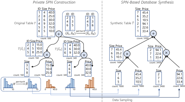
Figure 1 illustrates the process of constructing SPN for a single table and synthesizing data from it. Initially, the original table comprises two attributes and 500 rows. The data is partitioned into two groups of rows through clustering, which introduces a sum node. Subsequently, the columns within each group are separated by a product node, with each column forming a leaf node. Each leaf node stores a histogram representing its corresponding single-column subtable. To ensure DP, the table partition decision for the sum node, which consists of two sets of row indices or IDs, and the histogram for each leaf node are perturbed. During the data synthesis phase, synthetic data are sampled from these perturbed histograms and progressively merged up the hierarchy. A product node performs a horizontal concatenation of columns, while a sum node executes a vertical concatenation of rows. This recursive procedure is repeated until it reaches the root node, resulting in the generation of a complete synthetic dataset.
| Method | Input | Evalution Metric | Multi- table | DP | ||
| Query | DB | KL Div. | Card. error | ✓ | ||
| DPSynthesizer (li2014dpsynthesizer, ) | ✓ | high | medium | ✓ | ||
| DataSyn (ping2017datasynthesizer, ) | ✓ | high | high | ✓ | ||
| PrivSyn (zhang2021privsyn, ) | ✓ | high | high | ✓ | ||
| MST (mckenna2021winning, ) | ✓ | high | high | ✓ | ||
| PrivMRF (cai2021privmrf, ) | ✓ | high | high | ✓ | ||
| PreFair (pujol2022prefair, ) | ✓ | high | high | ✓ | ||
| AIM (mckenna2022aim, ) | ✓ | ✓ | high | high | ✓ | |
| SAM (yang2022sam, ) | ✓ | low | low | ✓ | ||
| PrivLava (cai2023privlava, ) | ✓ | low | medium | ✓ | ✓ | |
| VGAN (liu2023tabular, ) | ✓ | high | high | |||
| CGAN (liu2023tabular, ) | ✓ | high | medium | ✓ | ||
| PrivBench | ✓ | low | low | ✓ | ✓ | |
In essence, our contribution is a novel exploration into the equilibrium needed between synthesizing databases that maintain a high fidelity to original user data for DBMS benchmarking, while preserving user privacy. With smart incorporation of SPNs and DP, PrivBench provides a framework that aligns closely with benchmarking scenarios, protecting user privacy and reducing the compromise on the quality or authenticity of the synthesized database. Table 1 summarizes the comparison with alternative methods.
Our experimental results on several publicly accessible datasets demonstrate that PrivBench consistently achieves a uniformly lower query execution time error and Q-error on the cardinalities of queries compared to existing privacy-preserving data publishing methods such as PrivLava (cai2023privlava, ) with a notable reduction of up to 77%. Moreover, it surpasses SAM (yang2022sam, ), a data generation method without privacy preservation, exhibiting up to several orders of magnitude lower in Q-error and a 10-fold reduction in query execution time error. Regarding the KL divergence measured on the original and the synthetic databases, our method achieves improvements over PrivLava by 16% and SAM by 28%.
Our contributions are summarized as follows.
-
•
We study the problem of privacy-preserving database synthesis which transforms a database in a differentially private manner while aligning the performance of query workloads on the generated database with the original one.
-
•
To solve the problem, we propose PrivBench, which synthesizes databases by leveraging differentially private SPNs (Section 4). These SPNs ont only learn the data distributions of individual tables but also record the primary-foreign key references between them, adeptly managing complex dependencies among the relations in the input database.
-
•
We conduct a rigorous privacy analysis of PrivBench (Section 5). Our analysis proves that PrivBench satisfied DP and instructs how to allocate the privacy budget of DP within the complex and dynamic node construction process of the multi-SPN.
-
•
Experimental results illustrate that ours consistently achieves lower errors in query execution time and Q-errors in query cardinality, and exhibits improvements in KL divergence over alternative methods (Section 7).
2. Related Work
DP-based data synthesis stands as a significant solution to privacy-preserving data publication, with a plethora of relevant studies emerging in recent years (vietri2020new, ; aydore2021differentially, ; chen2020gs, ; ge2020kamino, ; li2014dpsynthesizer, ; li2021dpsyn, ; mckenna2021winning, ; mckenna2019graphical, ; zhang2017privbayes, ; zhang2021privsyn, ; snoke2018pmse, ; torkzadehmahani2019dp, ; xie2018differentially, ; cai2021privmrf, ). We classified these works into two categories based on their foundational methods.
GAN-based methods. Generative Adversarial Network (GAN) dominates the landscape of image generation techniques. Consequently, a prevailing trend in data synthesis involves the utilization of GANs and related variants (jordon2018pate, ; xie2018differentially, ; long2021g, ; liu2023tabular, ). The state-of-the-art approach outlined in (liu2023tabular, ) presents a solution named VGAN tailored for tabular data, which models tuples with mixed data types as numerical samples for subsequent deep learning model training. Building upon VGAN, Liu et al. (liu2023tabular, ) modified the discriminator, which directly accesses the original data, to satisfy differential privacy, resulting in the DP-compliant method CGAN.
Marginal set-based methods. According to the analysis presented in (tao2021benchmarking, ), marginal set-based methods (li2014dpsynthesizer, ; zhang2017privbayes, ; ping2017datasynthesizer, ; mckenna2019graphical, ; mckenna2021winning, ; cai2021privmrf, ; zhang2021privsyn, ; ge2020kamino, ; mckenna2022aim, ; pujol2022prefair, ; cai2023privlava, ) often demonstrate superior performance while adhering to privacy preservation. Early work DPSynthesizer (li2014dpsynthesizer, ) achieves synthetic data generation by building multivariate joint distribution. While the high-level designs of these methods share similarities, they diverge in their detailed approaches. PrivBayes (zhang2017privbayes, ), DataSyn (ping2017datasynthesizer, ) and PrivMRF (cai2021privmrf, ) opt for selecting specific subsets from -way marginals, where is determined by the dataset. In contrast, other mechanisms, such as MST (mckenna2021winning, ) and PrivSyn (zhang2021privsyn, ), maintain a fixed candidate set for 2-way marginal queries.
Moreover, PreFair (pujol2022prefair, ) introduces a causal fairness criterion, advocating for equitable fairness in the generated data. The novelty of AIM (mckenna2022aim, ) lies in being a workload-adaptive algorithm, which first selects a set of queries, conducts private measurements on these queries, and finally generates synthetic data from the noise measurements. PrivLava (cai2023privlava, ) builds upon the methodology of PrivMRF (cai2021privmrf, ) by also employing probabilistic graphical models (PGMs) for data modeling. However, what sets PrivLava apart from PrivMRF is its integration of latent variables, enabling it to effectively model foreign key constraints. Note that PrivLava stands as the current state-of-the-art method in this domain.
Outside the realm of DP-based data synthesis, there exist non-private approaches that support multi-table data synthesis (gilad2021synthesizing, ; yang2022sam, ), which we draw insights from. Among them, SAM (yang2022sam, ) stands out as the top performer. It devised a deep learning model for data synthesis, utilizing query workloads for training to produce a database that mirrors the original.
3. Problem Definition
| Type-ID | … |
| 1 | … |
| 2 | … |
| 3 | … |
| … | … |
| Range | … |
| ID | Size | Price | … | Type-ID |
| 1 | 4 | 40.0 | … | 1 |
| 2 | 8 | 25.0 | … | 1 |
| 3 | 6 | 30.0 | … | 2 |
| … | … | … | … | … |
| 498 | 9 | 32.0 | … | 9 |
| 499 | 3 | 15.0 | … | 10 |
| 500 | 5 | 10.0 | … | 10 |
| Range | [1, 10] | [0, 40.0] | … |
Consider a benchmark which consists of a database instance with its associated schema, each being a private relation table. For any , a tuple refers to a tuple , denoted as , if the foreign key of refers to the primary key of and the values of the two keys match. A tuple depends on , denoted as , if or there exist in , s.t. , , , , and . We assume never occurs in .
Without loss of generality, following previous work (cai2023privlava, ), we assume that is a primary private table (e.g., the table in Figure 2a) that contains sensitive information, and any other table , is a secondary private table (e.g., the table in Figure 2b) in which the tuples depend on the tuples in . We study the case of synthesizing a similar database to while preserving the privacy of all private tables. We employ differential privacy (DP) (dwork2014algorithmic, ; cai2023privlava, ), a celebrated approach for protecting database privacy.
Definition 0 (Differential Privacy (DP) (dwork2014algorithmic, ; cai2023privlava, )).
A randomized algorithm that takes as input a table (a database , resp.) satisfies -DP at the table level (at the database level, resp.) if for any possible output and for any pair of neighboring tables and (neighboring databases and , resp.),
| (1) | ||||
| (2) |
Two tables and neighbor if they differ in the value of only one tutple. and neighbor if can be obtained from by changing the values of a tutple and all other tuples that depend on .
Table-level DP provides a strong guarantee that the output distributions remain indistinguishable before and after any change to a single tuple . This should hold even when considering the dependencies among tuples induced by foreign keys in the relational schema. Therefore, we focus on database-level DP that further ensures that any change to the tuples that depend on should also has a limited impact on the output distributions. To ensure a bounded multiplicity for the neighboring databases, we follow prior work (kotsogiannis2019privatesql, ; tao2020computing, ; dong2022r2t, ; cai2023privlava, ) to assume that each tuple in is referred to by at most tuples for each secondary table . The privacy parameter controls the level of indistinguishability. With the definition of DP, we target the privacy-preserving database synthesis problem, defined as follows.
Problem 1 (Privacy-Preserving Database Synthesis).
Given a database with its schema, the task is to generate a database with the same schema as while ensuring -DP at the database level.
Whereas many privacy-preserving data synthesizers for DP are available, such as DPSynthesizer (li2014dpsynthesizer, ), PrivBayes (zhang2017privbayes, ), PrivSyn (zhang2021privsyn, ), PrivMRF(cai2021privmrf, ), and PrivLava (cai2023privlava, ), their aims are mainly reducing the error of aggregate queries (e.g., marginal queries (barak2007privacy, )), range queries, or downstream classification tasks, rather than publishing a database for benchmarking. Considering that the benchmark is used to test the performance of a DBMS, our aim is to synthesize a database with two concerns:
-
•
is supposed to be statistically similar to .
-
•
For the query workloads to be executed on , we expect they report the same runtime performance on .
For the first concern, one evaluation measure is KL divergence. Given a table and its counterpart , the KL divergence of from is defined as
where denotes the probability of tuple in . Then, the KL divergence of from is defined as the average KL divergence over all the tables of . For the second concern, given a query workload, we can compare the execution times on and . Since the execution time may vary across DBMSs, we can also compare the cardinality, i.e., the number of tuples in the query result, which is often used in a query optimizer for estimating query performance (leis2015good, ). In particular, Q-error (moerkotte2009preventing, ) is a widely used measure for comparing cardinalities:
where denotes a query in the workload, and and denote the cardinalities of executing on and , respectively. Then, we compute the mean Q-error of the queries in the workload.
4. PrivBench: Database Synthesis with Private SPNs
In this section, we propose PrivBench, an SPN-based differentially private database synthesis method.
4.1. Overview of PrivBench
PrivBench utilizes SPNs to address the two concerns outlined in Section 3. SPNs, due to their excellent performance in representing complex dependencies and data distributions at multiple granularities, have been employed in cardinality estimation (DeepDB, ), a prevalent approach intrinsically connected to estimating the runtime cost of queries. Drawing inspiration from this, we adapt the output in (DeepDB, ) to produce a synthesized database, designed to closely resemble the input database in terms of data distribution and cardinality upon query execution. As shown in Algorithm 1, PrivBench involves a three-phase process for database synthesis.
-
•
Private SPN Construction (Lines 1–2). Firstly, we construct an SPN for each table in the input database . Each SPN is created by a differentially private algorithm , where each leaf node contains a histogram of a column of a subset of rows in .
-
•
Private Fanout Construction (Lines 3–4). Secondly, we complement each SPN with some leaf nodes that model primary-foreign key references to obtain a modified SPN . We use a differentially private algorithm to calculate fanout frequencies for each foreign key and store them in the complemented leaf nodes.
-
•
SPN-Based Database Synthesis (Lines 5–6) Thirdly, we sample a table from each modified SPN to synthesize a database .
4.2. Private SPN Construction
4.2.1. Overview of
Algorithm 2 outlines our process for constructing an SPN on a single table. Following DeepDB (DeepDB, ), we employ a tree-structured SPN to model a given table . The procedure recursively generates a binary tree , where should be a parent node, and , should be two subtrees. We divide into the following three procedures.
-
•
(Operation Planning): We decide an operation for the parent node and the privacy budget allocated to .
-
•
(Parent Generation): According to the operation and the privacy budget , we generate the parent node.
-
•
(Children generation): We further generate the children , through recursive calls to .
4.2.2. Planning
The procedure takes the role of determining an operation for the parent node, which can be creating a leaf/sum/product node. A sum (resp. product) node indicates partitioning the rows (resp. columns) of the given table, while a leaf node means generating the table’s histogram. Since all these types of operations should be performed in a differentially private manner, also allocates a privacy budget for the parent node and calculates the remaining privacy budget for the children. Concretely, proceeds as follows.
1. Leaf node validation (Lines 1–2). We validate if we should only generate a leaf node for the given table. When both the size and the dimension of the given table are insufficient to split, i.e., and , the operation must be creating a leaf node, i.e., , and all the given privacy budget should be allocated for , i.e., . Here, we require that the size of a split subtable should not be smaller than the parameter for the sake of utility, which is ensured by the row splitting algorithm .
2. Correlation trial (procedure ). We preliminarily trial the performance of column splitting, which will be used to decide the operation by the procedure. Specifically, we consume a slight privacy budget to generate a trial column partition (Line 11) and compute the perturbed correlation
where calculates the normalized mutual information of two subtables, returns the global sensitvity of the given function, and generates the Laplace noise (Line 12). Intuitively, the smaller the correlation between the two subtables, the smaller the impact of column splitting on the data distribution, hence the better the performance of column splitting (DeepDB, ). Note that when either column or row splitting is infeasible, we do not need to evaluate the correlation since the operation must be the feasible one (Line 14).
Definition 0 (Column Splitting).
The column splitting mechanism outputs a column partition with probability proportional to , where is the set of all possible column partitions of , , and .
3. Operation decision (procedure ):. We determine the operation for the parent node. When the size (resp. dimension) of the table is insufficient for row (resp. column) splitting, the operation must be column (resp. row) splitting (Lines 22–25). However, when both column splitting and row splitting are feasible, we choose one of them according to the correlation (Lines 17–21). If does not exceed the threshold , we select column splitting as the operation because its performance is satisfactory.
4. Budget allocation (procedure ):. We allocate privacy budgets to the parent node and its children, respectively. Since nodes with less depth are more important for accurately modeling the data distribution, we allocate the privacy budget in a decreasing manner: always allocating half of the current privacy budget to the children, resulting in and (Line 31). However, when the operation is to split a table with only two attributes, since there is only one possible column partition, no privacy budget should be consumed for the parent node (Line 29).
4.2.3. Parent generation
Given the operation and its privacy budget , we generate the parent node as follows.
Case 1: . We generate a leaf node with a differentially private histogram (Line 7). Specifically, the procedure first computes a histogram over the table and then perturbs the histogram by adding some Laplace noise, which satisfies DP.
Case 2: . We call the procedure to create a sum node (Line 9). Here, can employ any differentially private K-means clustering algorithm (su2016differentially, ) to determine a perturbed row partition , where and are two clusters of row indices. Then, the partition is sotred in the sum node .
Case 3: . We apply the procedure to generate a product node (Line 11). Similar to the case of row splitting, determines a perturbed column partition to be stored in the node , and each element of the partition contains a subset of column indices. More concretely, as defined in Definition 1, employs an exponential mechanism to sample an instance of according its mutual information , which measures the correlation between ; the lower the mutual information, the higher the probability of outputting .
4.2.4. Children generation
If , the children are set to because the node is a leaf node (Line 19). Otherwise, we generate the and subtrees for the split subtables . Specifically, we first allocate the remaining privacy budget among the subtrees (Lines 14–17), which will be discussed in Section 5.1. Then, given the allocated privacy budgets , we call the procedure for the subtables to generate the subtrees , , respectively (Line 21).
4.3. Private Fanout Construction
After constructing SPNs for all private tables in the input database, we follow previous work (DeepDB, ; yang2022sam, ; yang2020neurocard, ) to utilize fanout distribution, i.e., the distribution of the foreign key in the referencing table, to model their primary-foreign key references. To maintain fanout distributions for all joined keys, prior work (DeepDB, ; yang2022sam, ; yang2020neurocard, ) uses a full outer join of all the tables, which causes large space overhead.
To address this issue, we propose Algorithm 4 that captures primary-foreign key references by complement SPNs with leaf nodes storing fanout distributions. Specifically, to construct the reference relation between tables and where refers to , we first find a certain attribute and traverse all its leaf nodes. For each leaf node , we identify the rows in whose column of attribute is stored in and count the fanout frequencies of the primary key of w.r.t. the identified rows, which a fanout table (Lines 3–5). Then, the fanout table is perturbed by adding some Laplace noise and stored in a new leaf node (Lines 6–7). Finally, we replace with a new subtree of SPN that connects and with a product node (Lines 8–9). Additionally, to minimize the impact of Laplace noise on the fanout distribution, we require attribute to have the most leaf nodes. Intuitively, the overall fanout distribution of a foreign key is the average of the fanout distributions stored in its leaf nodes. Therefore, the variance caused by the Laplace noise decreases as the leaf nodes increase.
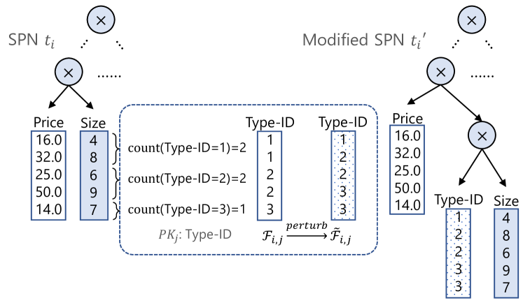
Example 2.
Figure 3 shows an example of how PrivBench complements the original SPN with the leaf nodes of the foreign key Type-ID. First, we identify that attribute size attribute possesses the most leaf nodes in . For each leaf node of attribute size, we find the corresponding subcolumn of attribute using the row indices of the subcolumn of attribute and calculate its fanout table. Then, we perturb the fanout table and store it in a new leaf node. Finally, the new leaf node is added into the SPN as a sibling to the leaf node of attribute and as the child of a newly added product node, resulting in a modified SPN .
4.4. SPN-Based Database Synthesis
Algorithm 5 shows how we synthesize a table given an SPN . If the root node of is a leaf node, we sample a table according to the histogram or fanout table stored in the node (Lines 1–2). If it is a sum (product, resp.) node, we recursively apply the procedure to the left and right children of and vertically (horizontally, resp.) concatenate the returned tables and (Lines 4–9). Finally, we obtain a table that has a data distribution similar to that of the private table . By synthesizing tables for all modified SPNs, we obtain a synthetic database .
5. Privacy Analysis
In this section, we rigoriously analyze how PrivBench satisfies DP and how we should allocate privacy budgets to some key steps in PrivBench.111All missing proofs can be found in our online appendix: https://drive.google.com/file/d/1mjhKOajBNvN5RbX7k_pvEoFi9DRCWuza/view?usp=sharing.
5.1. Privacy Analysis on
In this subsection, we first prove that the , , and procedures satisfy DP, and then prove that therefore achieves DP.
5.1.1. Analysis of
The procedure consists of the , , and subprocedures. If the subprocedures satisfy DP, we can conclude that ensures DP according to the sequential composition theorem of DP (dwork2006differential, ).
. (1) When and , the procedure employs the -DP procedure to compute a perturbed partition . Then, it calculates the NMI of and injects the Laplace noise into it, which ensures -DP. Consequently, according to the sequential composition theorem of DP (dwork2006differential, ), satisfies -DP. (2) When or , since varying the value of any row in does not have any impact on the output , satisfies -DP according to Definition 1. Note that we adopt the bounded DP interpretation; in the case of unbounded DP, adding/removing a row from causes the procedure to take the other conditional branch (i.e., Lines 11–14), thereby breaking the DP guarantee.
and . Similar to the second case of , for both procedures and , because changing the value of any row in does not affect the table size and the table dimension , it also does not impact their outputs. Therefore, they ensure -DP.
. When or , satisfies -DP since any change to does not impact the output (Lines 1–2); otherwise, since it sequentially combines , , and , satisfies the -DP according to the sequential composition theorem of DP (dwork2006differential, ), where the value of differs in different cases (see Lines 12 and 16).
Lemma 0.
For any and any , if and , satisfies -DP; otherwise, it satisfies -DP at the table level.
5.1.2. Analysis of
Then, we show that in any cases of the given operation , achieves DP. (1) When , we ensure DP using the Laplace mechanism. That is, we inject Laplacian noise into the histogram , which satisfies -DP. (2) When , we employ a DP row splitting mechanism to generate a perturbed row partition , which achieves -DP. (3) When , our column splitting mechanism is essentially an instance of the Exponential mechanism, thereby guaranteeing -DP.
Lemma 0.
For any and any , satisfies -DP at the table level.
5.1.3. Analysis of
Next, we analyze the DP guarantee of in different cases. (1) When , since always returns two null children, it must satisfy -DP. Therefore, in this case, achieves -DP. (2) When , Theorem 3 shows that in the case of row splitting, the privacy budgets for constructing the tree satisfies a parallel composition property:
Therefore, to optimize the utility of the subtrees, we maximize each subtree’s privacy budget and set . Note that Theorem 3 differs from the celebrated parallel composition theorem (dwork2006differential, ): their theorem assumes unbounded DP while our theorem considers bounded DP. (3) When , we allocate privacy budgets based on the scales of the subtrees (Line 18). Intuitively, a subtree with a larger scale should be assigned with a larger privacy budget to balance their utility. Thus, their privacy budgets are proportional to their scales . The scale metric is a function of the given table’s size and dimension, which will be defined in Theorem 6 based on our privacy analysis.
Theorem 3 (Parallel composition under bounded DP).
Given a row partition , publishing satisfies -DP at the database level, where is a subset of row indices and is a table-level -DP algorithm, .
Consequently, when or , we can prove the DP guarantee by mathematical induction: when (resp. ) returns a subtree with only a leaf node, as shown in case 1, it satisfies -DP (resp. -DP); otherwise, assuming (resp. ) satisfies -DP (resp. -DP), we conclude that satisfies -DP according to the sequential composition theorem (dwork2006differential, ) or Theorem 3, where or . Note that varying any row of does not affect and since they are functions of a table’s size and dimension.
Lemma 0.
For any , if , satisfies table-level -DP; otherwise, it satisfies table-level -DP.
5.1.4. Analysis of
Lemma 0.
For any , satisfies table-level -DP.
In addition, since allocates the privacy budget from the root to the leaf nodes in a top-down manner, it may result in insufficient budgets allocated to the leaf nodes. Consequently, an interesting question arises: If we allocate a privacy budget to all leaf nodes, how large the total privacy budget should be? Theorem 6 answers the question and instructs the design of the scale metirc. That is, if we guarantee a privacy budget for each leaf node, then constructing the and subtrees should satisfy -DP and -DP, respectively. Therefore, the privacy budgets should be proportional to the corresponding scales (see Line 17 of Algorithm 2). In our experiments, we set the scale metric as defined in Theorem 6 for .
Theorem 6.
Let denote the set of all possibles subtables of with and , . If for any , calls , satisfies table-level -DP, where .
5.2. Privacy Analysis on
For each leaf node , injects the Laplace noise into the fanout table (Line 5), which implements the -differentially private Laplace mechanism. Then, according to Theorem 3, publishing all the leaf nodes with perturbed fanout tables also satisfies -DP due to the nature of parallel composition. Therefore, ensures DP.
Lemma 0.
For any SPN , any primary key , and any , satisfies -DP at the table level.
5.3. Privacy Analysis on
Given that both and satisfy DP, the DP guarantee of the algorithm is established according to Theorem 8. Note that to measure the indistinguishability level of database-level DP, we cannot simply accumulate the privacy budgets assigned to each private table for table-level DP, i.e., . Intuitively, while table-level DP only guarantees the indistinguishability of neighboring tables, database-level DP requires indistinguishability of two tables that differ in at most tuples because those tuples may depend on a single tuple in the primary private table. Consequently, as shown in Corollary 9, the indistinguishability levels of procedures and at the table level should be reduced by factor for database-level DP. Therefore, to ensure -DP for , we can allocate the given privacy budget as follows:
where is the ratio of privacy budget allocated for fanout construction and is the number of all referential pairs . In our experiments, we follow the above setting of privacy budgets for PrivBench.
Theorem 8.
Given that satisfies -DP at the table level for all , satisfies -DP at the database level, where is the maximum multiplicity of .
Corollary 0 (of Theorem 8).
satisfies -DP at the database level.
| Dataset | #Tables | #Rows | #Attributes | Workload | Baselines | |||
| Adult | 1 | 48842 | 13 | SAM-1000 |
|
|||
| California | 2 | 2.3M | 28 | MSCN-400 | SAM (non-DP), PrivLava | |||
| JOB-light | 6 | 57M | 15 |
|
SAM (non-DP), DPSynthesizer |
6. Discussion
In this section, we discuss several interesting functionalities of PrivBench.
Supported data types
While most works on privacy-preserving database synthesis only support categorical data, PrivBench additionally supports numeric data. This is because the leaf nodes of the SPN can classify numeric data by range and generate histograms for these ranges. Synthetic numeric data is then sampled from these ranges using the histograms. Theoretically, this data synthesis method could also support more complex data types, such as text data and time series data, provided that we can divide the domain of the target data into meaningful subdomains to generate its histogram. Therefore, PrivBench is highly extensible, and its support for more data types could be a future research direction.
Visualization
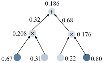
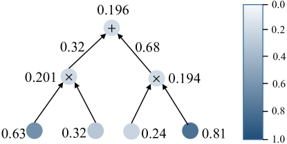
Visualization enable us to intuitively evaluate whether the data generated by PrivBench closely approximates the original data as a benchmark. As shown in Figure 4, after synthesizing data using PrivBench, we can obtain a pair of SPNs built on the original and synthetic data, respectively. After testing a bundle of queries, we can determine the selectivity value for each leaf node. Subsequently, we can color the leaf nodes based on the magnitude of the selectivity value, with darker colors indicating higher values, creating a colored SPN. Ultimately, by comparing the colored SPN of the original data with that of the synthetic data, we can assess whether the two sets of data perform similarly in benchmarking.
Benchmark scaling
In practice, users (e.g., companies) may require database benchmarks of different sizes to meet varying needs. Therefore, PrivBench supports synthesizing a database of any size by setting a scale factor for each table therein. However, determining an appropriate scale factor could be challenging for users lacking specialized knowledge, especially when their benchmarking requirements may evolve with the development of their business. Thus, a potential extension for PrivBench is to analyze the trends in the user’s historical query logs to predict their current needs and then automatically optimize scale factors for them. This approach would facilitate more tailored and efficient benchmarking adapted to the dynamic demands of users.
Composite foreign key
PrivBench also supports the synthesis of composite foreign keys. One possible method is to merge the multiple columns of a composite key into a single column and then generate leaf nodes for it. However, the merged column usually has a very large number of unique values, with each unique value having a very small count, which significantly impacts the utility of the histogram when some noise is injected. Therefore, we treat each column of the composite key independently. That is, we synthesize data independently for each column and then merge the synthetic columns to derive the synthetic composite key.
7. Experimental Evaluation
In this section, we conduct extensive experiments to demonstrate the effectiveness of PrivBench.
7.1. Experimental Settings
Research questions. Our experiments answer the following research questions.
-
•
Distribution similarity: Is the database synthesized by PrivBench closer to the original database in data distribution?
-
•
Runtime similarity: For executing query workloads, is the database synthesized by PrivBench closer to the original database in terms of runtime performance?
Datasets, query workloads, and baselines. Table 2 summarizes the datasets, query workloads, and baselines used to verify the performance of PrivBench, which are widely adopted in the database synthesis research. We introduce them as follows.
-
•
The Adult dataset contains a single table of census information about individuals, including their occupation and income. We utilize the preprocessed version provided in (yang2022sam, ). We execute SAM-100 (yang2022sam, ), a workload with 1000 randomly generated queries randomly, to evaluate the runtime performance of PrivBench and baselines. The baselines cover existing maintream data synthesis works, including non-private methods SAM (yang2022sam, ) and VGAN (liu2023tabular, ), and DP-based methods DPSynthesizer (li2014dpsynthesizer, ), DataSyn (ping2017datasynthesizer, ), MST (mckenna2021winning, ), PrivSyn (zhang2021privsyn, ), PrivMRF (cai2021privmrf, ), PreFair (pujol2022prefair, ), CGAN (liu2023tabular, ), and AIM (mckenna2022aim, ).
-
•
The California dataset (center2020integrated, ) consists of 2 tables about household information. We adopt MSCN-400 (kipf2018learned, ) as a query workload, containing 400 randomly generated queries with up to 2 joins. In addition to the non-private method SAM (yang2022sam, ), we employ PrivLava (cai2023privlava, ) as a baseline, which is an extension of PrivMRF (cai2021privmrf, ) for multi-relation synthesis.
-
•
The JOB-light dataset (yang2022sam, ) includes 6 tables related to movies, which is extracted from the Internet Movie Database (IMDB). In addition to the MSCN-400 workload with up to 2 joins, we also use the JOB-70 workload (yang2022sam, ), which focuses on joins of multiple tables and provides 70 queries with up to 5 joins. The baselines includes SAM (yang2022sam, ) and DPSynthesizer (li2014dpsynthesizer, ). Note that we do not test DPSynthesizer on California and PrivLava on JOB-light because their open-source code has not been adapted to these datasets.
These datasets are respectively used for single-relation, two-relation, and multi-relation database synthesis, thereby allowing for a comprehensive assessment of PrivBench’s performance.
| Model | KL Div. | Q-error | Exec. time error | ||||||||
| Mean | Median | 75th | 90th | MAX | Mean | Median | 75th | 90th | MAX | ||
| SAM | 6.48 | 1.97 | 1.31 | 1.76 | 2.70 | 168 | 0.52 | 0.38 | 0.62 | 0.81 | 1.68 |
| DPSynthesizer | 41.2 | 41.56 | 1.45 | 2.61 | 13.42 | 0.57 | 0.42 | 0.60 | 0.85 | 1.67 | |
| VGAN | 40.6 | 199.2 | 3.49 | 19.22 | 61.43 | 0.61 | 0.44 | 0.65 | 0.79 | 1.65 | |
| CGAN | 38.3 | 50.03 | 8.78 | 22.67 | 60.82 | 0.56 | 0.40 | 0.63 | 0.81 | 1.67 | |
| PrivSyn | 40.7 | 1519 | 28.39 | 576.3 | 4369 | 0.58 | 0.41 | 0.62 | 0.80 | 1.75 | |
| DataSyn | 39.5 | 426.9 | 13.81 | 95.74 | 568.0 | 0.55 | 0.44 | 0.63 | 0.82 | 1.69 | |
| PreFair | 33.5 | 381.4 | 13.47 | 103.8 | 518.6 | 0.63 | 0.48 | 0.67 | 0.86 | 1.75 | |
| MST | 35.1 | 833.5 | 20.22 | 246.3 | 1448 | 0.59 | 0.42 | 0.65 | 0.88 | 1.74 | |
| PrivMRF | 37.6 | 184.2 | 7.51 | 24.11 | 61.39 | 0.65 | 0.53 | 0.71 | 0.93 | 1.81 | |
| AIM | 34.8 | 766.4 | 16.54 | 161.2 | 882.1 | 0.59 | 0.47 | 0.68 | 0.82 | 1.66 | |
| PrivBench (sf=1) | 4.79 | 1.73 | 1.12 | 1.45 | 2.05 | 241 | 0.53 | 0.42 | 0.64 | 0.80 | 1.64 |
| PrivBench (sf=5) | 16.72 | 1.75 | 1.13 | 1.46 | 2.10 | 263 | 0.76 | 0.59 | 0.84 | 1.26 | 2.40 |
| PrivBench (sf=10) | 24.51 | 1.81 | 1.13 | 1.46 | 2.14 | 259 | 0.83 | 0.64 | 0.95 | 1.44 | 2.97 |
Metrics. To answer the first research question regarding distribution similarity, we employ the KL divergence defined in Section 3, which measures the difference in data distribution between the original and synthetic databases. Then, to answer the second research question regarding runtime similarity, we use Q-error defined in Section 3 and execution time error. While the former metric indirectly evaluates the runtime performance of the synthetic benchmark by calculating its error in the cardinality, the latter metric directly measures the difference in query execution time between the databases.
Settings of parameters. In our experiments, the privacy budget for PrivBench varies from to , which aligns with prior work (cai2023privlava, ). The settings of the scale metric and the privacy budgets for SPN construction and for fanout construction follow those discussed in Section 5. For all datasets, we set the threshold for column splitting , and the budget ratios for correlation trial. The minimum table size is set to for Adult and to for the other datasets considering that the table size of Adult in much smaller than other tables. The budget ratio for fanout construction is set to for California and to for JOB-light given that JOB-light has more referential pairs of tables to be connected by fanout tables.
Environment. All experiments are implemented in Python and performed on a CentOS 7.9 server with an Intel(R) Xeon(R) Silver 4216 2.10GHz CPU with 64 cores and 376GB RAM. The DBMS we use to test query execution is PostgreSQL 12.5 with 5GB shared memory and default settings for other parameters.
| Model | KL Div. | Q-error | Exec. time error | ||||||||
| Mean | Median | 75th | 90th | MAX | Mean | Median | 75th | 90th | MAX | ||
| SAM | 18.71 | 17.97 | 1.77 | 3.58 | 8.60 | 5040 | 1.19 | 0.75 | 1.07 | 1.48 | 2.16 |
| DPSynthesizer | 16.30 | 2355 | 1.02 | 1.598 | 14.39 | 1.11 | 0.66 | 1.01 | 1.43 | 2.21 | |
| PrivBench (sf=1) | 10.92 | 4.50 | 1.03 | 1.23 | 1.99 | 380 | 1.02 | 0.45 | 0.96 | 1.36 | 2.13 |
| PrivBench (sf=5) | 16.35 | 4.61 | 1.03 | 1.24 | 2.01 | 393 | 1.69 | 1.27 | 1.82 | 2.94 | 3.75 |
| PrivBench (sf=10) | 25.81 | 4.65 | 1.03 | 1.24 | 2.03 | 407 | 1.85 | 1.52 | 2.08 | 3.34 | 3.89 |
| Model | KL Div. | Q-error | Exec. time error | ||||||||
| Mean | Median | 75th | 90th | MAX | Mean | Median | 75th | 90th | MAX | ||
| SAM | 18.71 | 2776 | 2.29 | 5.39 | 27.78 | 110.7 | 1.03 | 5.81 | 86.47 | 6280 | |
| DPSynthesizer | 16.30 | 5963 | 3.35 | 46.91 | 478.7 | 106.2 | 0.83 | 4.57 | 59.92 | 5368 | |
| PrivBench (sf=1) | 10.92 | 15.85 | 1.30 | 2.61 | 5.77 | 923 | 13.17 | 0.52 | 2.85 | 5.49 | 636 |
| PrivBench (sf=5) | 16.35 | 16.68 | 1.32 | 2.78 | 5.92 | 1103 | 21.70 | 1.26 | 6.83 | 13.74 | 1261 |
| PrivBench (sf=10) | 25.81 | 16.94 | 1.32 | 2.82 | 6.11 | 1169 | 28.54 | 1.48 | 8.79 | 20.32 | 2658 |
7.2. Evaluation on Distribution Similarity
Adult. Table 3 shows the results on the Adult dataset. We can see that PrivBench outperforms all the baselines in terms of KL divergence Even when compared to non-DP methods, SAM and VGAN, the performance of PrivBench is still significantly better. In addition, we observe that PrivBench is sensitive to the scale factor , but even in the case of , its KL divergence is still much lower than those of DP-based baselines. Therefore, we conclude that PrivBench synthesizes statistically accurate databases in single-relation database synthesis. It is observed that there is no significant difference in this metric between GAN-based and Marginal-based approaches, highlighting the superiority of the intermediate structure, SPNs utilized in our work.
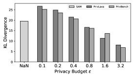
California. Figure 5a provides the KL divergences for PrivBench and PrivLava on the California dataset under different privacy budgets. The results indicate that PrivBench outperforms PrivLava for most values of privacy budget. Additionally, a higher privacy budget leads to a better KL divergence for both methods because less noise is injected into the database. Therefore, for two-relation databases, PrivBench can also synthesizes databases that are more similar to the original database in data distribution.
JOB-light. Tables 4 and 5 report the same results in KL divergence for dataset JOB-light because KL divergence is agnostic to the query workload. We have the following findings: First, when sf equals 1, the performance of PrivBench is not only better than DP-based baseline DPSynthesizer (li2014dpsynthesizer, ), but even better than the non-DP baseline SAM (yang2022sam, ). Then, increasing sf significantly hurts the KL divergence of PrivBench, but the loss is quite limited compared with the magnitude of scaling. Therefore, we conclude that for multi-relation database synthesis, the performance of PrivBench in terms of distribution similarity is also outstanding.
7.3. Evaluation on Runtime Similarity
Adult. The middle five columns of Table 3 present the results of experiments comparing our approach with other baselines on a single-table dataset in terms of Q-error-related metrics. The results demonstrate that PrivBench exhibits the lowest Q-errors across all metrics compared to other methods, including the non-DP baseline SAM. An additional encouraging observation is the minimal fluctuation of Q-error with respect to the scale factor (sf). Consequently, we conclude that our approach outperforms all baselines for single-relation synthesis in terms of Q-error, and its performance remains robust against increases in data scale.
Under the standard setting where the scale factor equals 1, our method exhibits lower execution time error compared to all other methods. Furthermore, we observed the scale factor has a significant impact on runtime performance. When the scale factor is increased to 5, PrivBench’s results no longer outperform those of the baseline methods. The relatively minor advantage of our work compared to other methods can be attributed to two main factors: firstly, the dataset’s small size, and secondly, the dataset containing only one single table, thus making the overall query tasks relatively straightforward. Subsequent experimental results corroborate this observation.
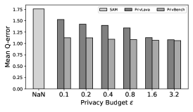
California. In Figure 5b, we illustrate the mean Q-error of SAM, PrivLava, and PrivBench in multi-table settings, and we observe the following trends: Firstly, in terms of overall performance, our method outperforms PrivLava, which in turn outperforms SAM. Secondly, there exists a linear correlation between privacy budget and Q-error: higher values of result in lower Q-error across different privacy budget scenarios. Thirdly, with lower values of , the difference between our method and PrivLava becomes more pronounced. This is due to the fact that our method consistently approaches the ideal scenario (Q-error = 1) with minimal fluctuation across privacy budgets, while PrivLava exhibits significant fluctuations. In conclusion, our method surpasses PrivLava in terms of Q-error, and its performance remains robust even with decreases in the privacy budget.
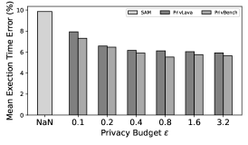
Similarly to the Q-error, in terms of execution time error, our work outperforms PrivLava and SAM. Additionally, both PrivLava and PrivBench exhibit a negative correlation between execution time error and privacy budget , indicating better runtime performance under larger privacy budget.
JOB-light. Tables 4 and 5 document the performance of baselines and PrivBench in terms of Q-error on the multi-table dataset JOB-light. We can observe that PrivBench consistently outperforms others, including SAM and DPSynthesizer, as evidenced in Tables 4 and 5. A comparison among Tables 3, 4, and 5, which respectively feature workloads with no joins, up to two joins, and up to five joins, illustrates that while the Q-error performance of SAM and DPSynthesizer deteriorates significantly with increasing joins, the performance of PrivBench remains stable. Consequently, it can be concluded that PrivBench not only surpasses DPSynthesizer in terms of Q-error but also demonstrates robust performance against increases in the number of joins.
In the multi-table experiment on execution time error, our approach significantly outperforms both competitors. As previously mentioned, our advantage increases significantly with the increase in dataset size and the number of joins between multiple tables, unaffected by the increase in scale factor. In conclusion, our approach excels over baselines in large multi-relation databases and remains robust against increases in scale factor.
7.4. Summary
Combining the experimental contexts of the three datasets and four sets of workloads mentioned earlier, PrivBench outperformed all DP-based and non-DP competitors in terms of KL divergence, Q-error, and execution time error. The performance of PrivBench is also robust against increases in data scale and decreases in privacy budget. This demonstrates that PrivBench can synthesize databases that are more similar to the original database in distribution and runtime performance. Additionally, as the number of joins increases, the advantages of PrivBench become more pronounced. In summary, our approach effectively balances data quality and privacy, presenting a promising solution to privacy-preserving database synthesis and benchmark publishing.
| Case study | KL Div. | Q-error |
|
||
| Estate database | 8.52 | 1.1 | 1.24 | ||
| Business database (sf=1) | 16.68 | 1.07 | 1.78 | ||
| Business database (sf=100) | 34.90 | 1.14 | 30.51 |
7.5. Case Study
In this subsection, we conduct two case studies to demonstrate the performance of PrivBench in real-world scenarios.
Case study 1: Real estate database. In this study, we select a real estate database (li2018homeseeker, ) collected from Australia, which provides a rich and diverse array of property-related information, including details about the properties themselves, addresses, surrounding features, school district information, and more. The database comprises 12 tables and various common data types. We construct 10 complex queries and evaluate the performance of PrivBench in terms of Q-error, KL divergence, and execution time error. As shown in Table 6, PrivBench performs excellently across all metrics, meeting practical needs. The query with the highest Q-error, targeting properties near the top 50 primary schools and their details, is:
"SELECT pb.*, pa.Formated Address, ps.name, sr.Ranking
FROM Property_Basic pb
JOIN Property_Address pa ON pb.proID = pa.proID
JOIN Mapping_School ms ON pb.proID = ms.pro_ID
JOIN School ps ON ms.sec1= ps.school_ID
JOIN School_Ranking sr ON ps.school_ID = sr.school_ID
WHERE sr.Ranking <= 50 and ps.type = ’Primary’;".
For this query, the cardinality on the original data was 2466, while on the generated data, it was 3129. The reason for this discrepancy is the noise perturbation on the Ranking and type attributes, with the error further amplified through the join of five tables, leading to the final cardinality difference. The execution time error for this query was 0.89 seconds, indicating that the query logic on the generated data did not undergo significant changes. The main cost still lies in the join of the five tables, and the changes in the two attributes did not significantly impact the table scan.
Case study 2: Real business database. In this study, we collaborate with CRDH, a large private company in China, to evaluate PrivBench in more complex scenarios. The company provides its benchmark for real business purposes, comprising 1,400 tables with a complex schema. The evaluation results in Table 6 demonstrate the outstanding performance of PrivBench in both distribution and runtime similarities when the data scale is not amplified. Additionally, the large-scale benchmark generated with a scale factor of also helped the company identify several system bottlenecks and design flaws, while other benchmarking tools are unable to achieve similar results.
8. Conclusion
In this paper, we delve into the domain of synthesizing databases that preserve privacy for benchmark publishing. Our focus is on creating a database that upholds differential privacy while ensuring that the performance of query workloads on the synthesized data closely aligns with the original data. We propose PrivBench, an innovative synthesis framework designed to generate data that is both high in fidelity and mindful of privacy concerns. PrivBench utilizes SPNs at its core to segment and sample data from SPN leaf nodes and conducts subsequent operations on these nodes to ensure privacy preservation. It allows users to adjust the granularity of SPN partitions and determine privacy budgets through parameters, crucial for customizing levels of privacy preservation. The data synthesis algorithm is proven to uphold differential privacy. Experimental results highlight PrivBench’s capability to create data that not only maintains privacy but also demonstrates high query performance fidelity, showcasing improvements in query execution time error, query cardinality error, and KL divergence over alternative approaches. The promising research directions for future work are twofold: (i) identifying the optimal privacy budget allocation scheme and (ii) generating data and query workloads simultaneously.
References
- [1] Tpc benchmarks. https://www.tpc.org/.
- [2] S. Aydore, W. Brown, M. Kearns, K. Kenthapadi, L. Melis, A. Roth, and A. A. Siva. Differentially private query release through adaptive projection. In ICML, pages 457–467. PMLR, 2021.
- [3] B. Barak, K. Chaudhuri, C. Dwork, S. Kale, F. McSherry, and K. Talwar. Privacy, accuracy, and consistency too: a holistic solution to contingency table release. In Proceedings of the twenty-sixth ACM SIGMOD-SIGACT-SIGART symposium on Principles of database systems, pages 273–282, 2007.
- [4] K. Cai, X. Lei, J. Wei, and X. Xiao. Data synthesis via differentially private markov random fields. PVLDB, 14(11):2190–2202, 2021.
- [5] K. Cai, X. Xiao, and G. Cormode. Privlava: synthesizing relational data with foreign keys under differential privacy. SIGMOD, 1(2):1–25, 2023.
- [6] M. Center. Integrated public use microdata series, international: Version 7.3 [data set]. minneapolis, mn: Ipums, 2020.
- [7] D. Chen, T. Orekondy, and M. Fritz. Gs-wgan: A gradient-sanitized approach for learning differentially private generators. NeurIPS, 33:12673–12684, 2020.
- [8] W. Dong, J. Fang, K. Yi, Y. Tao, and A. Machanavajjhala. R2t: Instance-optimal truncation for differentially private query evaluation with foreign keys. In Proceedings of the 2022 International Conference on Management of Data, pages 759–772, 2022.
- [9] C. Dwork. Differential privacy. In ICALP, pages 1–12. Springer, 2006.
- [10] C. Dwork, A. Roth, et al. The algorithmic foundations of differential privacy. Foundations and Trends® in Theoretical Computer Science, 9(3–4):211–407, 2014.
- [11] C. Ge, S. Mohapatra, X. He, and I. F. Ilyas. Kamino: Constraint-aware differentially private data synthesis. arXiv preprint arXiv:2012.15713, 2020.
- [12] A. Gilad, S. Patwa, and A. Machanavajjhala. Synthesizing linked data under cardinality and integrity constraints. In Proceedings of the 2021 International Conference on Management of Data, pages 619–631, 2021.
- [13] B. Hilprecht, A. Schmidt, M. Kulessa, A. Molina, K. Kersting, and C. Binnig. Deepdb: learn from data, not from queries! PVLDB, 13(7):992–1005, 2020.
- [14] J. Jordon, J. Yoon, and M. Van Der Schaar. Pate-gan: Generating synthetic data with differential privacy guarantees. In ICLR, 2018.
- [15] A. Kipf, T. Kipf, B. Radke, V. Leis, P. Boncz, and A. Kemper. Learned cardinalities: Estimating correlated joins with deep learning. arXiv preprint arXiv:1809.00677, 2018.
- [16] I. Kotsogiannis, Y. Tao, X. He, M. Fanaeepour, A. Machanavajjhala, M. Hay, and G. Miklau. Privatesql: a differentially private sql query engine. Proceedings of the VLDB Endowment, 12(11):1371–1384, 2019.
- [17] V. Leis, A. Gubichev, A. Mirchev, P. Boncz, A. Kemper, and T. Neumann. How good are query optimizers, really? PVLDB, 9(3):204–215, 2015.
- [18] H. Li, L. Xiong, L. Zhang, and X. Jiang. Dpsynthesizer: differentially private data synthesizer for privacy preserving data sharing. In PVLDB, volume 7, page 1677. NIH Public Access, 2014.
- [19] M. Li, Z. Bao, T. Sellis, S. Yan, and R. Zhang. Homeseeker: A visual analytics system of real estate data. Journal of Visual Languages & Computing, 45:1–16, 2018.
- [20] N. Li, Z. Zhang, and T. Wang. Dpsyn: Experiences in the nist differential privacy data synthesis challenges. arXiv preprint arXiv:2106.12949, 2021.
- [21] T. Liu, J. Fan, G. Li, N. Tang, and X. Du. Tabular data synthesis with generative adversarial networks: design space and optimizations. The VLDB Journal, pages 1–26, 2023.
- [22] Y. Long, B. Wang, Z. Yang, B. Kailkhura, A. Zhang, C. Gunter, and B. Li. G-pate: Scalable differentially private data generator via private aggregation of teacher discriminators. NeurIPS, 34:2965–2977, 2021.
- [23] R. McKenna, G. Miklau, and D. Sheldon. Winning the nist contest: A scalable and general approach to differentially private synthetic data. arXiv preprint arXiv:2108.04978, 2021.
- [24] R. McKenna, B. Mullins, D. Sheldon, and G. Miklau. Aim: An adaptive and iterative mechanism for differentially private synthetic data. arXiv preprint arXiv:2201.12677, 2022.
- [25] R. McKenna, D. Sheldon, and G. Miklau. Graphical-model based estimation and inference for differential privacy. In ICML, pages 4435–4444. PMLR, 2019.
- [26] G. Moerkotte, T. Neumann, and G. Steidl. Preventing bad plans by bounding the impact of cardinality estimation errors. PVLDB, 2(1):982–993, 2009.
- [27] H. Ping, J. Stoyanovich, and B. Howe. Datasynthesizer: Privacy-preserving synthetic datasets. In SSDBM, pages 1–5, 2017.
- [28] H. Poon and P. Domingos. Sum-product networks: A new deep architecture. In ICCV Workshops, pages 689–690. IEEE, 2011.
- [29] D. Pujol, A. Gilad, and A. Machanavajjhala. Prefair: Privately generating justifiably fair synthetic data. arXiv preprint arXiv:2212.10310, 2022.
- [30] J. Snoke and A. Slavković. pmse mechanism: differentially private synthetic data with maximal distributional similarity. In PSD, pages 138–159. Springer, 2018.
- [31] D. Su, J. Cao, N. Li, E. Bertino, and H. Jin. Differentially private k-means clustering. In Proceedings of the sixth ACM conference on data and application security and privacy, pages 26–37, 2016.
- [32] Y. Tao, X. He, A. Machanavajjhala, and S. Roy. Computing local sensitivities of counting queries with joins. In Proceedings of the 2020 ACM SIGMOD International Conference on Management of Data, pages 479–494, 2020.
- [33] Y. Tao, R. McKenna, M. Hay, A. Machanavajjhala, and G. Miklau. Benchmarking differentially private synthetic data generation algorithms. arXiv preprint arXiv:2112.09238, 2021.
- [34] R. Torkzadehmahani, P. Kairouz, and B. Paten. Dp-cgan: Differentially private synthetic data and label generation. In CVPR Workshops, pages 0–0, 2019.
- [35] G. Vietri, G. Tian, M. Bun, T. Steinke, and S. Wu. New oracle-efficient algorithms for private synthetic data release. In ICML, pages 9765–9774. PMLR, 2020.
- [36] L. Xie, K. Lin, S. Wang, F. Wang, and J. Zhou. Differentially private generative adversarial network. arXiv preprint arXiv:1802.06739, 2018.
- [37] J. Yang, P. Wu, G. Cong, T. Zhang, and X. He. Sam: Database generation from query workloads with supervised autoregressive models. In SIGMOD, pages 1542–1555, 2022.
- [38] Z. Yang, A. Kamsetty, S. Luan, E. Liang, Y. Duan, X. Chen, and I. Stoica. Neurocard: one cardinality estimator for all tables. PVLDB, 14(1):61–73, 2020.
- [39] J. Zhang, G. Cormode, C. M. Procopiuc, D. Srivastava, and X. Xiao. Privbayes: Private data release via bayesian networks. ACM Transactions on Database Systems, 42(4):1–41, 2017.
- [40] L. Zhang, C. Chai, X. Zhou, and G. Li. Learnedsqlgen: Constraint-aware sql generation using reinforcement learning. In SIGMOD, pages 945–958, 2022.
- [41] Z. Zhang, T. Wang, N. Li, J. Honorio, M. Backes, S. He, J. Chen, and Y. Zhang. PrivSyn: Differentially private data synthesis. In USENIX Security, pages 929–946, 2021.