Distributed Representations Enable
Robust Multi-Timescale Computation
in Neuromorphic Hardware

Abstract

Programming recurrent spiking neural networks (RSNNs) to robustly perform multi-timescale computation remains a difficult challenge. To address this, we show how the distributed approach offered by vector symbolic architectures (VSAs), which uses high-dimensional random vectors as the smallest units of representation, can be leveraged to embed robust multi-timescale dynamics into attractor-based RSNNs. We embed finite state machines into the RSNN dynamics by superimposing a symmetric autoassociative weight matrix and asymmetric transition terms. The transition terms are formed by the VSA binding of an input and heteroassociative outer-products between states. Our approach is validated through simulations with highly non-ideal weights; an experimental closed-loop memristive hardware setup; and on Loihi 2, where it scales seamlessly to large state machines. This work demonstrates the effectiveness of VSA representations for embedding robust computation with recurrent dynamics into neuromorphic hardware, without requiring parameter fine-tuning or significant platform-specific optimisation. This advances VSAs as a high-level representation-invariant abstract language for cognitive algorithms in neuromorphic hardware.

I Introduction

Neuromorphic computing promises to match the efficiency of information processing in the brain by emulating biological neural and synaptic dynamics in hardware [1]. In contrast to more conventional artificial neural networks (ANNs), biological neurons have rich internal temporal dynamics and interact sparsely with unary events (spikes). Performing multi-timescale tasks – such as motor planning and execution – with biologically-plausible spiking neurons requires information to be retained and processed for periods much longer than the timescales available in individual neurons and synapses [2, 3]. Information must then be represented by the collective dynamics of recurrently-connected populations of neurons instead. Programming recurrent spiking neural networks (RSNNs) to perform long-timescale tasks with short-timescale neurons remains a formidable challenge however, due to the conflicting demands that the network should react quickly to input but otherwise be stable on long timescales [4].

In the face of these challenges, a possible approach would be to apply gradient-based iterative learning algorithms to train the network parameters to solve a particular task [5, 6, 7]. However, besides being computationally intensive and biologically implausible, such approaches are not well-suited to tasks with long timescales, due to the need to backpropagate gradients into the distant (potentially infinite) past [8]. Furthermore, these approaches do not have guarantees of stability and robustness, compared to those afforded by much simpler biologically-inspired models like the Hopfield attractor network [9, 10].

If the trained networks are to be deployed on mixed-signal neuromorphic hardware, one must usually perform calibrating chip-in-the-loop training, lest device-specific nonidealities absent during training lead to a catastrophic degradation in network performance upon deployment [11, 12, 13, 14, 6]. To overcome these difficulties and to shift to more robust training procedures, it has been suggested that a more appropriate level of description for programming neuromorphic hardware may be at the level of high-dimensional patterns of neuron activity, rather than individual neuron and synapse parameters [15]. In vector symbolic architectures (VSAs) – also known as hyperdimensional computing (HDC) – arbitrary symbolic data structures are represented by high-dimensional random vectors, known as hypervectors, such that information is distributed across the entire vector [16, 17, 18, 19]. The representations are thus not dependent upon the precise functioning of individual components, which is a critical property for robust functioning in neuromorphic hardware and biology [20, 21].

In this work, we show how the VSA approach of using hypervectors as the smallest unit of representation can be leveraged to program arbitrary state machines into RSNNs in a scalable and robust manner. Neural state machines have already been shown to be important computational primitives for reproducing cognitive behaviours in neuromorphic agents [22], and have been used in the context of solving constraint satisfaction problems [23]. We represent each state with a hypervector and store it in the RSNN as a fixed-point attractor. The VSA formalism allows us to superimpose additional heteroassociative outer-product terms within the weight matrix, without causing substantial interference. These additional terms embed the input-triggered transitions between attractor states.

We first embed multiple state machines into simulated RSNNs with non-ideal synaptic weights. To validate these simulations in neuromorphic hardware, we create a proof-of-concept implementation using a memristive crossbar setup run in a closed-loop with simulated neurons. Finally, we implement these networks on Intel’s asynchronous digital neuromorphic research chip Loihi 2 [24], to demonstrate the algorithm’s scalability.

This work demonstrates the capability of VSAs as a functional abstraction layer for neuromorphic hardware [15]. It permits the description of complex RSNN behaviours from a high level while being invariant to the choice of underlying neural representation, and is highly robust to hardware-specific non-idealities. It is a step towards a general framework for interoperability of cognitive algorithms across varying neuromorphic hardware architectures, without requiring significant optimisation or fine-tuning upon deployment to each particular platform.

II Results

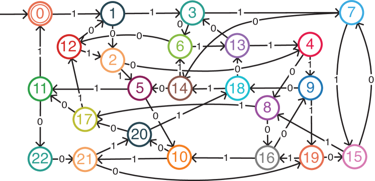
Figure 1: The 23-state DFA embeded into RSNNs in simulation and on Loihi 2. This particular DFA performs modulo division of binary numbers. The DFA is initialised in the state $q_{0}$, and a binary number is input most-significant-bit first. The final state indicates the result of the input $\mathrm{mod}\>\>23$.

State machines are perhaps the most comprehensive model of multi-timescale dynamics, as they react quickly to input but are otherwise stable on indeterminately-long timescales. They also have a clear utility for building more complex neural models of cognitive behaviours [22, 25, 23]. We focus on the task of embedding deterministic finite automata (DFAs) into recurrent spiking neural networks (RSNNs) by expressing the DFA in terms of high-dimensional attractor states and transitions between them. For every state $q$ in the finite set of states $Q$, we embed an associated fixed-point attractor state in the RSNN dynamics that is stable on long timescales. When input is given to the network, the RSNN should quickly transition between attractor states according to the desired state transition function $F:Q\times S\rightarrow Q$ in the DFA, where $S$ is the set of all input symbols.

We achieve this by IID generating hypervectors $\mathbf{\bm{q}}\in\{0,1\}^{N}$ to represent each DFA state $q$, then storing this state in the RSNN’s dynamics using a Hopfield-like outer-product learning rule. The vectors follow a sparse block structure, i.e., the $N$ elements are split up into $M$ blocks of equal length $L$, and exactly one entry in each block is nonzero [26, 27].

We use sparse rather than dense vectors to benefit from the increased capacity in attractor networks [28, 29, 30], distributed rather than localist for robustness [31], and random and pseudo-orthogonal rather than perfectly orthogonal due to the number of available states being exponential rather than linear in $N$ (Section S3) [32]. We use a sparse block structure due to the simplicity of the required neural activation function, and compatibility with the VSA framework [27]. Additionally, we move closer to a more biologically-plausible model of attractor transition dynamics in the brain, where sparse representations enforced by local competitive mechanisms are abundant [33, 34].

For every state transition, we embed additional outer product terms such that if the correct subset of neurons is masked by external input, the RSNN may transition between attractor states (see Methods). The terms are of the form $(\mathbf{\bm{q}}_{1}-\mathbf{\bm{q}}_{0})(\mathbf{\bm{q}}_{0}\circ\overline{\mathbf{\bm{s}}})^{\intercal}$ where $\overline{\mathbf{\bm{s}}}$ is another (bipolar) hypervector, and “$\circ$” is a VSA binding operation. Without input to the network, these terms are pseudo-orthogonal to the network state, i.e. $\langle(\mathbf{\bm{q}}_{0}\circ\overline{\mathbf{\bm{s}}})\cdot\mathbf{\bm{q}}_{0}\rangle=0$ and so have negligible effect. When the network is masked by the correct (binary) hypervector $\mathbf{\bm{s}}$ however (effectively an unbinding operation), they become similar to the network state, i.e. $(\mathbf{\bm{q}}_{0}\circ\overline{\mathbf{\bm{s}}})\cdot(\mathbf{\bm{q}}_{0}\land\mathbf{\bm{s}})=\frac{1}{2}M$ where “$\land$” is component-wise $\mathrm{AND}$, implementing the masking. This allows us to effectively modulate the strengths of superimposed terms by masking neurons in the RSNN [21].

We then wish to program this weight matrix onto neuromorphic hardware to reliably and robustly realise the desired dynamics without requiring significant optimisation or adaptation to the target hardware. In contrast, deployment of RSNNs to neuromorphic hardware usually requires some degree of chip-in-the-loop training or post-deployment fine-tuning to ensure robustness to hardware-specific nonidealities [12, 11, 6, 35, 36]. This requirement severely limits the ability of neuromorphic hardware to be deployed at scale.

We demonstrate the reliability and generality of our approach by running experiments in three SNN environments. First in simulation, where we show the ideal functioning of the RSNN even with considerably non-ideal weights. Second, a closed-loop memristive hardware setup with 64$\times$64 resistive RAM (RRAM) devices acting as the synaptic weights, demonstrating the suitability of the approach for novel beyond-CMOS memristor-integrated neuromorphic hardware. Third, we demonstrate on Intel’s neuromorphic research chip Loihi 2 that the approach scales up seamlessly to large state machines.

II-A SNN simulation

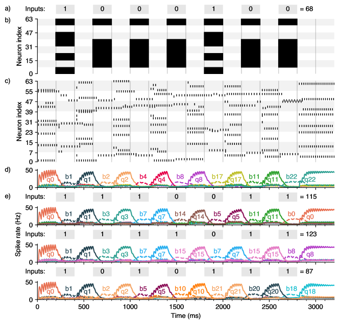
Figure 2: An RSNN performing a walk on the 23-state DFA, using noisy 1-bit weights. a) The symbolic input to the RSNN. b) The input vector to the RSNN at any time, which each masks out half of the neurons therein. Each different input $s$ corresponds to a different hypervector $\mathbf{\bm{s}}$. Only the first 64 neurons are shown. c) A spike raster plot of activity within the RSNN. When the input to the network is constant, the network stabilises in an attractor state. When the input changes, some blocks are masked out or revealed, which may cause transitions to a new attractor state. The WTA mechanism ensures that only one neuron is persistently active in each block. d) The kernel-filtered mean firing rate of the neurons active in the attractor states $\mathbf{\bm{q}}_{0},\ldots,\mathbf{\bm{q}}_{22}$, as well as the transition-facilitating bridge states $\mathbf{\bm{b}}_{0},\ldots,\mathbf{\bm{b}}_{22}$. The bridge states are represented by dashed lines and coloured the same as their corresponding $q$ attractor states. Interpreting the sequence of inputs given as a binary number, the final inhabited attractor state indicates the result of the number modulo 23. We here serially input the number 68, and the RSNN correctly halts in the $q_{22}$ state. e) The same RSNN is given different sequences of inputs, and the RSNN performs the correct walk between attractor states in all cases.

The simulated RSNN consists of $N$ leaky integrate-and-fire (LIF) neurons, with all-to-all synaptic connectivity, except between neurons in the same block, which have Winner-Take-All (WTA) connectivity between themselves (see Methods). This enforces that only one neuron in each block may spike at once, thereby restricting the neural activity to have a sparse block code structure.

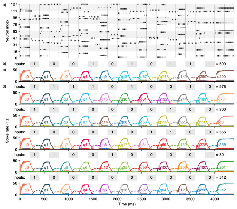
Figure S3: A 300-state DFA embedded into an RSNN in simulation with ideal weights. The chosen DFA implements modular division of binary numbers by 300, generated in the same way as in Figures 1 and 2. a) A raster plot of the first 64 neurons’ spikes, with block length $L=16$. b) The symbolic inputs to the RSNN. c) The mean firing rate of the neurons in each attractor state. d) Different input sequences are given to otherwise identical simulations. In all cases, the RSNN performs the correct walk between attractor states, with the final inhabited state indicating the result of the input binary number $\mathrm{mod}\ 300$. By specifying our RSNN dynamics in the VSA framework, scaling up the algorithm to large state machines is seamless, and is limited only by the memory capacity of the attractor network.

Although the method generalises to arbitrary DFAs [21], we chose to implement a 23-state DFA which can perform modular division of binary numbers (Figure 1), as it is a clear example of useful computation. Two inputs, $s_{0}$ and $s_{1}$, with associated random hypervectors $\mathbf{\bm{s}}_{0}$ and $\mathbf{\bm{s}}_{1}$, are input to the network to represent “0” and “1”, respectively. A sequence of inputs thus corresponds to a dividend $d$ in binary representation, and the final state corresponds to the result of the modular division $d\ \mathrm{mod}\ 23$. The full state transition function is described by the transitions $q_{n}\overset{s_{0}}{\longrightarrow}q_{(2n\ \mathrm{mod}\ 23)}$ and $q_{n}\overset{s_{1}}{\longrightarrow}q_{(2n+1\ \mathrm{mod}\ 23)}$ for all states $q_{n}$, $n\in\{0,\ldots,22\}$. The weight matrix to implement this DFA was constructed as described in Methods. We then stochastically binarized the ideal weights and added independently-sampled Gaussian noise of standard deviation 0.5 to each binary weight value, such that the two weight distributions were highly overlapping. This demonstrates robustness to low-precision and noisy weights, which are inherent in most neuromorphic hardware platforms. Despite these nonidealities, the RSNN performs the correct walk between attractor states for every input sequence (Figure 2). A similar DFA with 300 states (Figure S3) was constructed in the same way, to demonstrate the seamless scaling to large state machines.

II-B Memristive crossbar

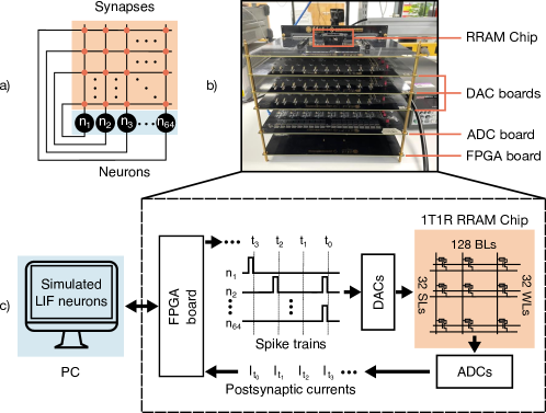
Figure 3: The closed-loop experimental setup for running the RSNN using the 4K RRAM system. a) A simplified schematic of the 64-neuron RSNN. b) The physical RRAM measurement system, containing an FPGA board, three DAC boards and one ADC board. c) The scheme of running the closed-loop experiment in which the LIF neurons are simulated on a PC. The FPGA board receives the control commands from the PC and operates all word-, source- and bit lines (WLs, SLs, BLs) of the RRAM chip in parallel. At each time step ($t_{n}$), the spikes generated by the neurons are sent to the synapse array on WLs, which are represented by voltage pulses. Meanwhile, a 0.2V read voltage is applied to the SLs. The postsynaptic currents ($I_{t_{n}}$) produced by the RRAM cells accumulate on each BL, and the readout results are returned to the PC through the ADCs and FPGA.

To demonstrate that the approach is robust to non-idealities introduced by memristive devices, we run a closed-loop experiment with synapses on a memristive crossbar and neurons in simulation (Figure 3). Whenever the simulated neurons spiked, the memristive crossbar was read by applying the binary vector of spiking neurons as a voltage input vector to the crossbar via the on-board DACs. The readout currents were read by the ADCs and then fed back into the simulation as postsynaptic currents. With this hybrid “computer in the loop” approach, we demonstrate the readiness of the algorithm for implementation on emerging SNN-memristor platforms [37].

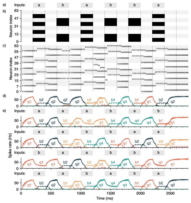
Figure S4: The closed-loop memristive crossbar experiment, configured to embed a second DFA. The DFA is given by $q_{0}\overset{a}{\rightarrow}q_{1}\overset{a}{\rightarrow}q_{2}\overset{b}{\rightarrow}q_{3}\overset{b}{\rightarrow}q_{0}$. a) The symbolic input to the network. b) The masking input to the network, with a separate mask for $a$ and $b$. Due to size constraints, the mask vectors were chosen to be orthogonal. c) The spiking activity of neurons within the RSNN. d) The mean firing rates of the neurons within each attractor state. e) The same experiment was performed with different sequences of inputs, which cause corresponding different walks between the states. The RSNN performs the correct walk between attractor states in all cases. Although there is erroneous neuron firing in some blocks (due to the non-ideal device conductances), the distributed states ensure the overall dynamics are unaffected.

We used an RRAM crossbar with 4096 devices. Due to this size constraint, we implemented smaller DFAs than in simulation. The weights were mapped to ternary values by thresholding, and then written to three conductance states on the RRAM devices. Although the device programming procedure in principle supports more weight states – limited by the precision of the ADCs (12 bit) – relaxation effects in the filamentary RRAM cause the conductance values to disperse in the milliseconds to seconds after programming, reducing the effective precision of the weights [38, 39]. After this dispersion, the RRAM devices store the synaptic weights in a non-volatile fashion [40]. We first implemented a DFA representing a 4-state counter. The RSNN performs the correct walk between attractor states, despite the fixed-pattern-noise and trial-to-trial weight non-idealities in the crossbar current readouts (Figure 4). We then implemented another 4-state DFA but with two inputs, following an identical procedure. For every input sequence tested, the network performs the correct walk between attractor states (Figure S4).

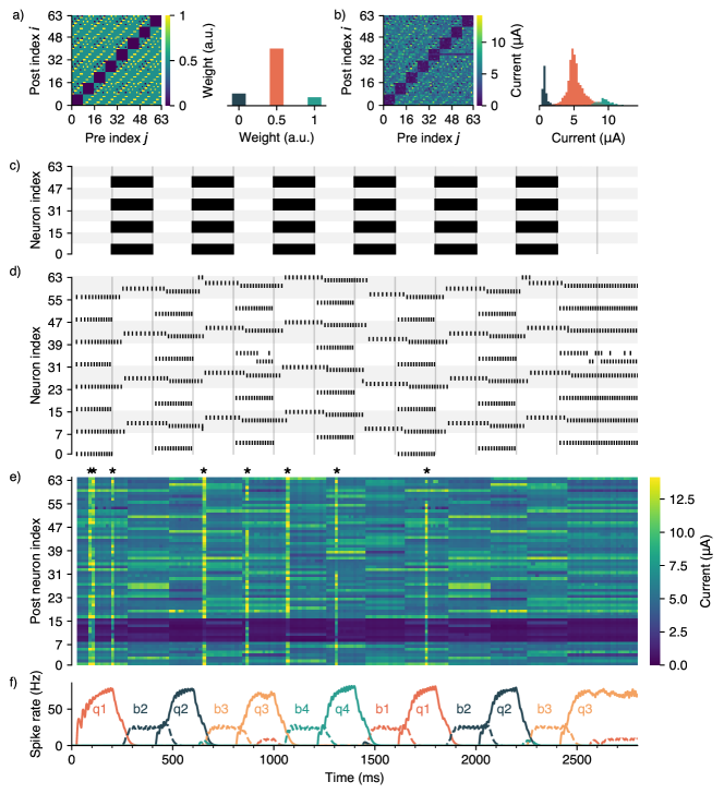
Figure 4: A 4-state DFA embedded into an RSNN using a memristive crossbar with 64$\times$64 RRAM devices as the synaptic weights. The DFA is described by $q_{0}\overset{s}{\rightarrow}q_{1}\overset{s}{\rightarrow}q_{2}\overset{s}{\rightarrow}q_{3}\overset{s}{\rightarrow}q_{0}$ for a single input $s$. a) The ternary weight matrix to be written to the RRAM crossbar, and a histogram of the values. b) Readout currents from each of the 64$\times$64 RRAM devices after programming, and separate histograms for each of the ternary weight values. There is significant mismatch between the measured currents and the ideal values; a row of faulty devices which give almost no current; and devices which give anomalously large currents. c) The masking input to the network. d) A spike raster plot of the neurons within the RSNN. Due to the size constraints introduced by the crossbar, we chose the attractor hypervectors $\mathbf{\bm{q}}$ to be orthogonal rather than random. e) Measured postsynaptic current readings from whenever a neuron in the second block spiked, chosen for the prominence of trial-to-trial current variation. The weights between neurons in the same block were programmed to the lowest weight, hence the horizontal band of low currents. At some times, multiple neurons fired within the same time step (labelled by asterisks above). f) The mean firing rates of the neurons in each attractor state. Despite the considerable nonidealities present, the RSNN performs the correct walk between attractor states.

II-C Loihi 2

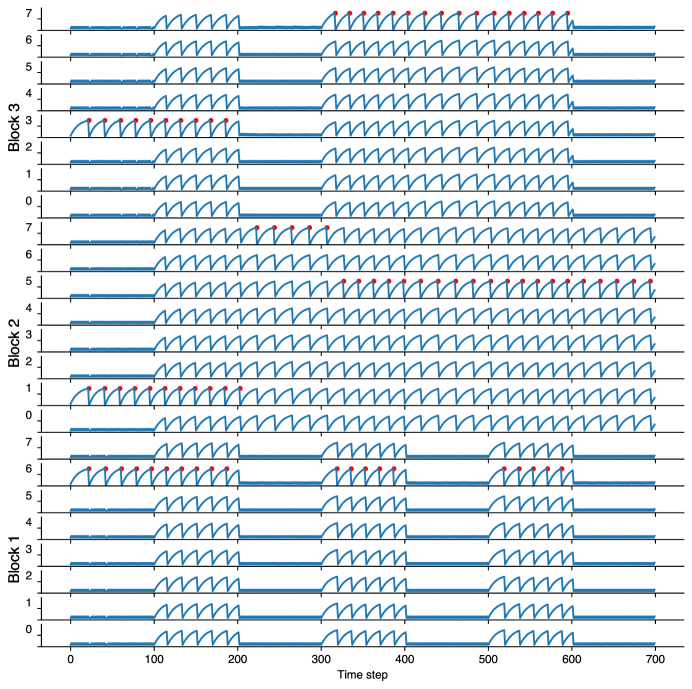
Figure S2: The winner-take-all mechanism implemented on Loihi 2. Although every neuron is receiving enough excitatory input that it will spike if unhindered, the WTA mechanism - implemented using shunting inhibition - allows only the neuron with the greatest integrated current to spike. This is an easy way to stabilize the attractor dynamics and constrains the neural activity to sparse block codes.

To demonstrate that the approach scales to large state machines on neuromorphic hardware and can be easily transferred to different types of neuromorphic systems, we implemented the RSNN on Intel’s neuromorphic research chip Loihi 2. We implemented a functionally-equivalent block-WTA mechanism with shunting inhibition synapses using a custom neuron microcode. This is required to give each neuron both a conventional integrative synapse and a shunting inhibition synapse. When a shunting synapse is stimulated, it resets the membrane potential of the target neuron to a subthreshold value (Figure S2), implementing the within-block WTA and the block-wise masking of the RSNN by input. The integrative synapses implement the recurrent weight matrix as specified in Methods. We implemented the same 23-state DFA as in simulation (Figure 1), now quantizing the ideal weights to the available 8-bit values.

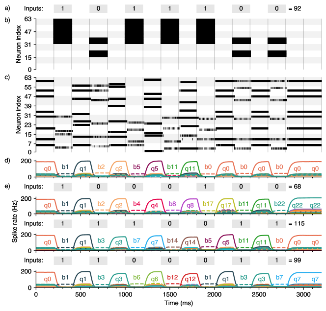
Figure 5: The 23-state DFA on Loihi 2. a) The input symbol to the network at any time, and b) the corresponding input vectors, which mask the network activity. c) A spike raster plot of the first 64 neurons. The shunting-inhibition WTA mechanism ensures that only one neuron in every block may spike at once (see Methods). d) Kernel firing-rate estimates of each $q$ and $b$ state, choosing arbitrarily that 1 time step on Loihi represents 1ms. The sequence of inputs given corresponds to the binary representation of the number 92. The RSNN halts in the $q_{0}$ state, indicating correctly that 92 is divisible by 23. e) For all sequences of inputs, the correct walk between attractor states is performed.

The network performs the correct walk between attractor states reliably for all given input sequences (Figure 5).

III Discussion

It is a widely-held belief that recurrent attractor dynamics underlie the brain’s ability to temporarily represent information in stable neuron firing patterns, without the need for components with intrinsically-long timescales [41], and despite the non-idealities present in biological systems [42, 43, 44, 45, 3].

Networks that switch between discrete attractor states are used to explain neural recordings and are thought to underlie higher decision-making processes [46, 47, 48, 25]. These robust dynamics inspired the embedding of controlled attractor transition dynamics in RNNs, in particular in neuromorphic systems that mimic the brain’s parallelism and asynchrony, but suffer from a similar inherent unreliability of single components as biological systems [49] (see [21] for a more comprehensive overview).

In previous efforts to embed attractor-based state machines into spiking neuromorphic hardware [22, 23], each state was represented by a dedicated orthogonal (non-overlapping) population of neurons with a synaptic gating mechanism to trigger state transitions. Although this simplifies the state encoding, these localist state representations limit the robustness, flexibility and scalability of the network in comparison to a distributed approach [31]. If each state is represented by a unique population of $M$ neurons that are active for only one pattern, then a network of $N$ neurons can represent at most $N/M$ patterns. In contrast, sparse distributed single-layer attractor networks can store $N^{2}/(\log{N})^{2}$ patterns, making more efficient use of the available synaptic resources [29, 30, 28]. Additionally, adding new states with localist representations requires adding or finding new neurons which are inactive for every other pattern. This is at odds with the mixed selectivity of neurons found throughout the brain [50].

We instead utilised the distributed representational framework of Vector Symbolic Architectures (VSAs), with which it has been shown possible to achieve the approximately quadratic scaling for state machines embedded into RNNs [21]. In VSAs, symbolic data is represented by high-dimensional random vectors which can be composed to represent arbitrary data structures and algorithms [16]. The state-representing hypervectors thus have a nonzero probabilistic degree of overlap, but it is nonetheless possible to generate an exponential (in $N$) number of hypervectors for which significant overlap between any pair of hypervectors is unlikely (Section S3) [32, 51].

The distributed representation also makes the network highly robust to various nonidealities, such as noise, individual component failure and non-ideal neuron dynamics. Their robustness to low-precision (quantized) and inaccurate synaptic weights is particularly relevant for memristive in-memory applications. Along with the flexibility of VSAs, this has prompted recent interest in combining VSAs with memristive crossbars [20, 52] and spiking neural networks [53, 54, 55, 56], where synaptic and neural non-idealities are abundant. The results obtained from simulations and the closed-loop memristive crossbar setup confirm the system’s reliable operation under hardware constraints, notably without requiring parameter fine-tuning.

The VSA binding operation let us construct the recurrent weight matrix for a particular DFA, by superimposing autoassociative and heteroassociative outer-product terms without incurring considerable interference. Transitions are triggered by masking a subset of the neurons – constituting an effective unbinding operation – while in previous work, additional mechanisms were required to modulate between attractor and transition dynamical regimes [57, 58, 59, 60, 61, 62, 63, 64]. Furthermore, the simplicity of this construction method means that the weight matrix could reasonably be learned via local Hebbian learning rules, such that states and transitions are learned and unlearned as needed to solve a particular task [65].

Programming a certain DFA into an RSNN in one shot may be sufficient for some applications, however. In space, ionizing solar radiation causes unwanted bit-flips in systems using conventional charge-based memories, and so necessitates fault-tolerant computation schemes. Our system is intrinsically robust to such events, since the attractor dynamics quickly reverse any erroneous flips in the neural state. Furthermore, RRAM-based memories are highly resistant to solar radiation, making memristive VSA-programmed attractor-based neuromorphic implementations of conventional algorithms potentially suitable for space and other high-energy applications [66].

The flexibility and robustness of the model enables a wide range of applications for neuromorphic hardware. It could be used to coordinate information flow in complex neuromorphic systems [67], or be directly incorporated into existing works leveraging VSA representations [68], such as online learning of robotics schemas [69] or general computation with VSA-based stack machines [70, 15].

By adopting the VSA formalism, we programmed an RSNN from an abstract higher level of description, which is separated from the exact details of the hardware. It relied on the existence of a fixed stereotypical low-level neural motif (the block-WTA connectivity), but adjusted only the connections between neurons in different blocks, to easily program the same neural hardware for different purposes. This ability to abstract the function of lower layers and then build upon them relatively carefree is the foundation of conventional digital design approaches and bears resemblance to Marr’s levels of analysis [71, 15]. VSAs are especially suited as an abstraction layer to divorce high-level function from low-level neural dynamics, in part due to their invariance of the choice of hypervector representation [15, 16]. For example, in place of sparse block code hypervectors, we could have instead used phasor hypervectors [72, 18] or their sparse variants, which have an elegant connection to the periodic spiking of resonate-and-fire neurons [53, 54]. The same VSA-based algorithm could be implemented on different neuromorphic hardware platforms, using whichever hypervector representation is best suited for the available neuron circuit. Neuromorphic computing would greatly benefit from a high-level neurally-inspired abstract programming language, which can be robustly implemented across different neuromorphic hardware platforms [73, 15, 74]. Although there have been many works towards such a unification [75, 76, 77, 78, 79], the majority of these focus on finding common ways to interface with different neuromorphic hardware platforms, or to compose functional SNN modules, rather than on defining higher-level abstract primitives that are invariant of the neural representations on the hardware on which they are embedded.

This work serves as a demonstration of the broader argument that VSAs are a highly capable level of abstraction for embedding computation through neural dynamics into neuromorphic hardware [15]. We embedded arbitrary state machines into RSNNs, as they are a clear example of multi-timescale computation: the switching between states is fast, but the attractor dynamics ensure stability on long timescales [9, 10]. The fully-distributed representations ensure increasing robustness with increasing dimensionality and can be composed to represent arbitrary data structures and algorithms. Their invariance to the choice of hypervector representation – many of which have elegant spiking implementations – may allow neuromorphic hardware to be programmed at a level that is entirely divorced from the underlying neural representations, but that can reliably and robustly be implemented on different neuromorphic hardware platforms without the need for fine-tuning.

IV Methods

IV-A VSA arithmetic

Vector symbolic architectures (VSAs) are a way to represent compositional data structures in a distributed manner, using high-dimensional random vectors, hypervectors, as the smallest units of representation [16, 19, 17, 18]. They rely on the fact that independently-generated high-dimensional vectors have a very small inner product (the so-called pseudo orthogonality property) and so they can be iteratively generated to represent new items. The simplest hypervectors are balanced bipolar hypervectors $\mathbf{\bm{x}}\in\{-1,1\}^{N}$, where the value $X_{i}$ at any component in a hypervector $\mathbf{\bm{x}}$ is IID generated via $P(X_{i}=1)=P(X_{i}=-1)=0.5$, known as the Multiple-Add-Permute (MAP) VSA model [19, 16]. We define the similarity between any pair of MAP hypervectors by the normalised inner product, $\mathrm{sim}(\mathbf{\bm{x}},\mathbf{\bm{y}})=\frac{1}{N}\mathbf{\bm{x}}\cdot\mathbf{\bm{y}}$. The similarity between a hypervector and itself is then $\mathrm{sim}(\mathbf{\bm{x}},\mathbf{\bm{x}})=1$, while the similarity between independently-generated hypervectors is approximately 0 with standard deviation $1/\sqrt{N}$. For large $N$, any significant similarity between hypervectors thus conveys meaning, since it is overwhelmingly unlikely that the similarity occurred unintentionally [17, 32].

Each VSA model is equipped with (at least) two operators to generate hypervectors which represent relationships between other hypervectors, and so also the symbols they represent. They are known as bundling ($\oplus$) and binding ($\circ$), often corresponding to component-wise addition and multiplication respectively. The hypervector produced by a bundling operation is similar to its constituents, $\mathrm{sim}(\mathbf{\bm{a}}\oplus\mathbf{\bm{b}},\mathbf{\bm{a}})\approx\mathrm{sim}(\mathbf{\bm{a}}\oplus\mathbf{\bm{b}},\mathbf{\bm{b}})\approx 1$, and so can be used to represent sets. The hypervector produced by a binding operation is dissimilar to both of its constituents: if $\mathbf{\bm{c}}=\mathbf{\bm{a}}\circ\mathbf{\bm{b}}$, then $\mathrm{sim}(\mathbf{\bm{c}},\mathbf{\bm{a}})\approx\mathrm{sim}(\mathbf{\bm{c}},\mathbf{\bm{b}})\approx 0$. But, $\mathbf{\bm{c}}$ has the property that either of its constituents may be used as an inverse, to extract the other via an unbinding operation. In the MAP VSA model, the Hadamard product (element-wise multiplication) serves as both the binding and unbinding operations. It is then clear that $\mathbf{\bm{b}}$ can be retrieved from $\mathbf{\bm{c}}$ via $\mathbf{\bm{c}}\circ\mathbf{\bm{a}}=\mathbf{\bm{b}}$ and vice versa.

The simplest example of a data structure built using VSAs is a store of key-value pairs (also known as role-filler bindings). Given a finite set of keys $k\in K$ and values $v\in V$, we can generate for every $k$ and $v$ a hypervector $\mathbf{\bm{k}}_{k}$ and $\mathbf{\bm{v}}_{v}$ to represent them. A hypervector $\mathbf{\bm{m}}$ may then be constructed to unambiguously represent a datastore $g:K\rightarrow V$ of key-value pairs, by superimposing a set of bound hypervectors via

$$\mathbf{\bm{m}}=\bigoplus_{\text{keys }k}\mathbf{\bm{k}}_{k}\circ\mathbf{\bm{v}}_{g(k)}$$ (1)

To find the value associated with a given key $l\in K$, we bind to $\mathbf{\bm{m}}$ the key hypervector $\mathbf{\bm{k}}_{l}$, giving $\mathbf{\bm{m}}\circ\mathbf{\bm{k}}_{l}=\mathbf{\bm{v}}_{g(l)}\oplus\bigoplus_{\text{keys }k\neq l}\mathbf{\bm{k}}_{k}\circ\mathbf{\bm{k}}_{l}\circ\mathbf{\bm{v}}_{g(l)}$. The terms in the summation are not similar to any hypervector in our codebooks for $K$ or $V$, and so produce inner products of order $\mathcal{O}(1/\sqrt{N})$ only. This hypervector is thus just the desired value hypervector $\mathbf{\bm{v}}_{g(k)}$, plus a summation of noise terms. A “clean” version of the value hypervector can be obtained by an autoassociative cleanup memory, for example an attractor network with energy minima at the states $\mathbf{\bm{v}}$ [80, 81]. We can also simply read out the represented value $v$ by choosing the $\mathbf{\bm{v}}_{v}$ with the greatest inner product with $\mathbf{\bm{m}}\circ\mathbf{\bm{k}}_{g(l)}$, via an exhaustive search or more efficient methods [82, 83]. Although this is a simple example of how compositional data structures can be represented, it is the foundation for solving more interesting tasks with VSAs, such as reasoning by analogy or compositional visual reasoning problems [54, 84, 85].

We make use of both dense bipolar (MAP) hypervectors and sparse binary block code (SBC) hypervectors [26, 19, 16]. Although SBC hypervectors have their own canonical binding operation [27], in this work we liberally mix the SBC and MAP models to realise the desired RSNN dynamics. By exploiting the pseudo-orthogonality of bound hypervectors, we construct the recurrent weights by superimposing different associative weights matrices, without incurring significant interference between them. The masking-out of neurons in the RSNN constitutes an effective unbinding operation. Terms which are bound to an input hypervector, and so were pseudo orthogonal, may effectively be unbound, thereby becoming aligned, which allows us to trigger state transitions by selectively masking neurons with input.

IV-B State machine embedding

A DFA is a finite state machine containing a set of states $Q$, an initial state $q_{0}\in Q$, a finite set of input symbols $S$, and a state transition function $F:Q\times S\rightarrow Q$. In addition, a DFA denotes a subset $A\subseteq Q$ of its states as “accepting” states. A string of input symbols is then said to have been accepted by the DFA if it terminates in one of the acceptance states. As such, DFAs can be used to perform pattern matching – accepting or rejecting strings based on a predefined set of rules, regular expressions [86].

The DFA is embedded into the attractor network by first generating for each state $q\in Q$ a binary hypervector $\mathbf{\bm{q}}\in\{0,1\}^{N}$ to represent this state. We restrict these hypervectors to be sparse block codes. That is, we divide the $N$ components into $M$ equally-sized blocks of length $L=N/M$ (we choose $N$ to be divisible by $M$ for our convenience), and then let exactly one component in each block be $1$-valued, with the rest $0$. The state hypervectors $\mathbf{\bm{q}}$ are then stored as attractors in the RSNN in one shot via a sparse generalization of the Hebbian outer-product learning rule in Hopfield networks [29, 30, 28].

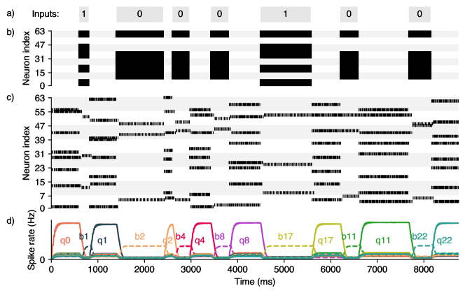
Figure S5: The simulated RSNN with an irregular input timing scheme. a) The symbolic input to the network. inputs were given for between 200ms and 1000ms. b) The corresponding input hypervector masking the neurons. c) A raster plot of spike activity in the RSNN. d) The mean firing rate of the neurons in each attractor state. The network is not reliant on an exact input timing scheme to perform the correct sequence of transitions. There is, of course, a minimum duration for which an input (or lack thereof) must be given, to ensure the postsynaptic currents have time to update, which is determined by the synaptic time constant $\tau_{\text{syn}}$.

Additional terms are required to embed the correct state-transition dynamics. For every input symbol $s\in S$, a dense binary hypervector $\mathbf{\bm{s}}\in\{0,1\}^{N}$ is generated, which, when input to the network, should trigger the correct transitions between attractor states. We restrict these hypervectors to be block-constant, such that components in the same block have the same value. We will denote $\bar{\mathbf{\bm{s}}}\in\{-1,1\}^{N}$ as the equivalent bipolar representation of these hypervectors, given by $\bar{\mathbf{\bm{s}}}=2\mathbf{\bm{s}}-1$. For every state $q$, an additional sparse binary block-coded vector $\mathbf{\bm{b}}$ is generated, which we refer to as its bridge state. They will be attractors of the RSNN dynamics only when there is input to the network. Transitions will be constructed such that, when we give input to the RSNN, it will not transition directly from a source state $\mathbf{\bm{q}}$ to target state $\mathbf{\bm{q}}^{\prime}$, but rather will transition from $\mathbf{\bm{q}}$ to $\mathbf{\bm{b}}^{\prime}$, the bridge state belonging to the target state $\mathbf{\bm{q}}^{\prime}$. When the input is removed, the RSNN will finally flow from the $\mathbf{\bm{b}}^{\prime}$ to $\mathbf{\bm{q}}^{\prime}$ state, completing the transition. Splitting each transition up in this way ensures they are not dependent upon a specific input timing scheme (Figure S5). For the sake of understanding, the construction of the recurrent weight matrix $\mathbf{W}\in R^{N\times N}$ can be divided into three parts, first to embed the $\mathbf{\bm{q}}$ states as attractors

$$\begin{split}\mathbf{W}_{\text{attr.}}=\sum_{q\in Q}(\mathbf{\bm{q}}-f)(\mathbf{\bm{q}}-f)^{\intercal}\end{split}$$ (2)

where the coding level $f=1/L$ is the fraction of nonzero elements in each $\mathbf{\bm{q}}$ hypervector. This is the same weight description for storing sparse attractors as in earlier works [30, 29]. We then embed the dynamics of the bridge states, via

$$\begin{split}\mathbf{W}_{\text{brdg.}}=\sum_{q\in Q}\Big{[}&(\mathbf{\bm{q}}-f)(\mathbf{\bm{b}}-f)^{\intercal}\\ +&\sum_{s\in S}(\mathbf{\bm{b}}-\mathbf{\bm{q}})\big{(}(\mathbf{\bm{b}}-f)\circ\bar{\mathbf{\bm{s}}}\big{)}^{\intercal}\Big{]}\end{split}$$ (3)

where “$\circ$” is the Hadamard product (component-wise multiplication). We are thus using an unorthodox mixture of the MAP [19] and SBC [26, 27] VSA models [16]. These terms cause the bridge states $\mathbf{\bm{b}}$ flow to their corresponding $\mathbf{\bm{q}}$ states, except when input is present, then they themselves become attractors of the RSNN’s dynamics. In order to store transitions between states, outer product terms are then similarly added for each non-loop transition, the set of which we define as $E=\{(q,s,q^{\prime})\>\ \text{s.t.}\ \>q^{\prime}=F(q,s),\>q^{\prime}\neq q\}$. They are included as

$$\begin{split}\mathbf{W}_{\text{trans.}}=\sum_{\eta\in E}(\mathbf{\bm{b}}^{\prime}-\mathbf{\bm{q}})\big{(}(\mathbf{\bm{q}}-f)\circ\bar{\mathbf{\bm{s}}}\big{)}^{\intercal}\end{split}$$ (4)

where $\mathbf{\bm{q}}$ is the attractor state for source state $q$ for edge $\eta$, and $\mathbf{\bm{b}}^{\prime}$ the bridge state belonging to the target state $q^{\prime}=F(q,s)$, as defined by $E$. The full weight matrix is then given by the superposition $\mathbf{W}=\mathbf{W}_{\text{attr.}}+\mathbf{W}_{\text{brdg.}}+\mathbf{W}_{\text{trans.}}$.

IV-C RSNN attractor dynamics

While no input is given to the network, the states $\mathbf{\bm{q}}$ are attractors of the network dynamics, and the bridge states $\mathbf{\bm{b}}$ immediately transition to their corresponding $\mathbf{\bm{q}}$ state. When input is given to the network, which we implement as masking of the network state, terms inside $\mathbf{W}$ which were pseudo-orthogonal to the network state, may become similar. The currently-inhabited state may cease to be an attractor of the dynamics, and may instead drive the network to a different attractor state. In simulation, the masking operation is implemented by input-triggered refractory periods, and on Loihi by shunting inhibition synapses.

If $\mathbf{W}$ contained only the symmetric attractor terms $\mathbf{W}_{\text{attr.}}$, then we could consider the dynamics of the network when each block is updated asynchronously in discrete time steps, where one block is picked at random, and the neuron with the greatest input spikes. The RSNN can then be coarsely described by a neural state vector $\mathbf{\bm{z}}_{t}\in\{0,1\}^{N}$, indicating which neuron is active in each block. Due to the symmetry of $\mathbf{W}^{\text{attr.}}$, we can define an energy

$$E(\mathbf{\bm{z}}_{t})=-\frac{1}{2}\mathbf{\bm{z}}_{t}^{\intercal}\mathbf{W}_{\text{attr.}}\mathbf{\bm{z}}_{t}$$ (5)

which will either decrease or stay the same between time steps (Section S1) [87]. By construction, our energy surface consists of energy wells at our DFA states $\mathbf{\bm{q}}$, which gives us our much-revered fixed-point attractor dynamics [30, 29].

This description of the dynamics is only valid when ignoring the asymmetric terms present in $\mathbf{W}$. To describe the dynamics due to the addition of the other terms, we consider the postsynaptic sum $\mathbf{\bm{h}}_{t+1}=\mathbf{W}\mathbf{\bm{z}}_{t}$ with and without an input to the RSNN. It is instructive to work with the expectation of $\mathbf{\bm{h}}_{t+1}$, where terms containing inner products between independent hypervectors can be discarded. We must, however, keep in mind that for finite $N$, the postsynaptic sum will only approximate its expected value, due to the accumulation of nonzero inner products between realised hypervectors. See [32, 51] for a rigorous theoretical analysis. We first consider the dynamics when the network is in an attractor state, $\mathbf{\bm{z}}_{t}=\mathbf{\bm{q}}^{\mu}$ for some $q^{\mu}\in Q$. The expected postsynaptic sum $\langle\mathbf{\bm{h}}\rangle$ is then given by

$$\begin{split}\langle\mathbf{\bm{h}}\rangle&=\bigl{\langle}\mathbf{W}\mathbf{\bm{q}}^{\mu}\bigr{\rangle}\\ &=\bigl{\langle}\mathbf{W}_{\text{attr.}}\mathbf{\bm{q}}^{\mu}\bigr{\rangle}+\bigl{\langle}\mathbf{W}_{\text{brdg.}}\mathbf{\bm{q}}^{\mu}\bigr{\rangle}+\bigl{\langle}\mathbf{W}_{\text{trans.}}\mathbf{\bm{q}}^{\mu}\bigr{\rangle}\\ &\propto(\mathbf{\bm{q}}^{\mu}-f)+\mathbf{\bm{0}}+\mathbf{\bm{0}}\\ &=\mathbf{\bm{q}}^{\mu}-f\end{split}$$ (6)

where only the terms inside $\mathbf{W}_{\text{attr.}}$ give a nonzero contribution. The terms inside $\mathbf{W}_{\text{brdg.}}$ can be ignored because the $\mathbf{\bm{b}}$ and $\mathbf{\bm{q}}$ hypervectors are all mutually pseudo-orthogonal. In $\mathbf{W}_{\text{tran.}}$ there are terms including the $\mathbf{\bm{q}}$ hypervectors, and so one might expect $\mathbf{W}_{\text{tran.}}$ to contribute to $\langle\mathbf{\bm{h}}\rangle$. However, the VSA binding operation in each of the summed terms (Equation 4) produces hypervectors which are pseudo-orthogonal to $\mathbf{\bm{q}}^{\mu}$, i.e. $\langle(\mathbf{\bm{q}}-f)\circ\bar{\mathbf{\bm{s}}})\cdot\mathbf{\bm{q}}^{\mu}\rangle=0\>\forall\>\mathbf{\bm{q}},\mathbf{\bm{q}}^{\mu}$. The superimposed $\mathbf{W}_{\text{tran.}}$ matrix thus does not contribute to the expected postsynaptic sum $\langle\mathbf{\bm{h}}\rangle$, it is effectively hidden by the VSA binding operation. See Section S2 for a derivation. In the large-$N$ limit, and sufficiently close to the attractor states $\mathbf{\bm{q}}$, we thus have only the fixed-point attractor dynamics resulting from the symmetric $\mathbf{W}_{\text{attr.}}$ matrix [30, 29].

IV-D RSNN transition dynamics

We now consider how $\langle\mathbf{\bm{h}}\rangle$ changes when we apply an input $s^{\lambda}\in S$ to the RSNN, which we assume corresponds to a valid transition $\eta=(q^{\mu},s^{\lambda},q^{\mu\prime})\in E$ from state $q^{\mu}$ to $q^{\mu\prime}$. Inputting $s^{\lambda}$ to the RSNN corresponds to applying $\mathbf{\bm{s}}^{\lambda}\in\{0,1\}^{N}$ as a mask to the RSNN, such that all neurons in the blocks for which $\mathbf{\bm{s}}^{\lambda}$ is zero are prevented from spiking. The expected postsynaptic sum is then given by

$$\begin{split}\langle\mathbf{\bm{h}}\rangle&=\bigl{\langle}\mathbf{W}(\mathbf{\bm{q}}^{\mu}\land\mathbf{\bm{s}}^{\lambda})\bigr{\rangle}\\ &=\bigl{\langle}\mathbf{W}_{\text{attr.}}(\mathbf{\bm{q}}^{\mu}\land\mathbf{\bm{s}}^{\lambda})\bigr{\rangle}+\bigl{\langle}\mathbf{W}_{\text{brdg.}}(\mathbf{\bm{q}}^{\mu}\land\mathbf{\bm{s}}^{\lambda})\bigr{\rangle}\\ &\quad\quad+\bigl{\langle}\mathbf{W}_{\text{trans.}}(\mathbf{\bm{q}}^{\mu}\land\mathbf{\bm{s}}^{\lambda})\bigr{\rangle}\\ &\propto(\mathbf{\bm{q}}^{\mu}-f)+\mathbf{\bm{0}}+(\mathbf{\bm{b}}^{\mu\prime}-\mathbf{\bm{q}}^{\mu})\\ &=\mathbf{\bm{b}}^{\mu\prime}-f\end{split}$$ (7)

where $\land$ is a component-wise $\mathrm{AND}$ operation, implementing the masking. The RSNN thus transitions to the $\mathbf{\bm{b}}^{\mu\prime}$ state, the bridge state belonging to the target $q^{\mu\prime}$ state. By applying $\mathbf{\bm{s}}^{\lambda}$ as a mask to the RSNN, we caused heteroassociative terms to be projected out of the edge summation in $\mathbf{W}_{\text{trans.}}$, which push the RSNN from $\mathbf{\bm{q}}^{\mu}$ to $\mathbf{\bm{b}}^{\mu\prime}$.

A similar calculation can be done to show that the bridge states $\mathbf{\bm{b}}$ are attractors only when the network is being masked by a valid input, i.e. $\langle\mathbf{W}(\mathbf{\bm{b}}^{\mu}\land\mathbf{\bm{s}})\rangle=\mathbf{\bm{b}}^{\mu}-f$. When the input is removed, however, this becomes $\langle\mathbf{W}\mathbf{\bm{b}}^{\mu}\rangle=\mathbf{\bm{q}}^{\mu}-f$, driving the RSNN towards the target $\mathbf{\bm{q}}$ state, completing the transition. By applying a sequence of inputs to the RSNN as masks (with pauses in between), we cause the RSNN to perform the desired sequence of transitions between attractor states. Including the bridge states in the state machine construction ensures that transitions are not dependent upon a specific input timing scheme, since an input must be given – and crucially then removed – to complete a transition (Figure S5) [21]. If an input $s$ were given that did not correspond to a valid transition for the current state $q$, no transition occurs.

Constructing attractor networks with transition dynamics by superimposing symmetric autoassociative terms and asymmetric heteroassociative terms, is not a new idea [57]. In order to ensure that neither attractor or transition dynamics dominated always, one had to either ensure a fine balance between the relative strengths of the two terms [58, 59, 88], or to introduce additional mechanisms to modulate their relative strengths, such as delayed synapses [60, 61, 62, 89] or short-term synaptic plasticity [63, 64]. By exploiting the properties of VSAs, we have achieved the same result without such mechanisms and without sacrificing robustness. By adding to $\mathbf{W}$ latent heteroassociative terms which were each bound to a certain hypervector $\mathbf{\bm{s}}$, in the absence of input, we could ignore their contribution to the RSNN dynamics, due to the zero expected inner product with the network state (Equation 6). However, when we mask the RSNN with the same $\mathbf{\bm{s}}$ – an effective unbinding operation – these heteroassociative terms are revealed, and trigger the transition dynamics (Equation 7). We use the masking mechanism to realise an unbinding operation because it is not reliant on the synchronous arrival of inputs [21].

It is important to emphasize that the synaptic weights are never altered during operation. Rather, by selectively excluding columns of $\mathbf{W}$ from the dynamics, we change which states project to which.

IV-E Spiking neuron model

We simulate leaky integrate-and-fire neurons (LIF), defined by

$$\frac{\mathrm{d}u_{i}}{\mathrm{d}t}=-\frac{1}{\tau_{m}}(u_{i}-u_{\text{rest}})+\frac{1}{C}I_{i}(t)$$ (8)

where $u_{i}$ is dynamical membrane voltage of the neuron $i$, $\tau_{m}$ and $u_{\text{rest}}$ are the membrane time constant and rest potential respectively, $I_{i}$ is the postsynaptic current to that neuron, and $C=\qty{1}{F}$. When $u$ exceeds the spiking threshold $u_{\theta}$, the neuron emits a spike and $u$ is quickly clamped to a subthreshold reset voltage (here 0mV) for an amount of time determined by the refractory period $\tau_{\text{ref}}$. The postsynaptic currents $I_{i}(t)$ we modelled as second-order low-pass filters over spike inputs,

$$\begin{split}\tau_{\text{syn}}\frac{\mathrm{d}I_{i}}{\mathrm{d}t}&=-I_{i}+J_{i}(t)\\ \tau_{\text{syn}}\frac{\mathrm{d}J_{i}}{\mathrm{d}t}&=-J_{i}+\sum_{j=1}^{N}w_{ij}\sum_{\text{spks }k}\delta(t-t_{j}^{k})\end{split}$$ (9)

where we introduce the synaptic time constant $\tau_{\text{syn}}$, the Dirac delta function $\delta(\cdot)$, and we sum over the spike times $t_{j}^{k}$ from all presynaptic neurons $j$, with synaptic weight $w_{ij}$ measured in coulombs. This has solution

$$\begin{split}I_{i}(t)&=\sum_{j=1}^{N}w_{ij}\Big{(}K(t)\circledast\sum_{k}\delta(t-t^{k}_{j})\Big{)}(t)\\ &=\big{[}\mathbf{W}\mathbf{\bm{z}}(t)\big{]}_{i}\end{split}$$ (10)

where $K(t)$ is an exponentially-decaying alpha kernel with time constant $\tau_{\text{syn}}$, $\circledast$ indicates temporal convolution, and $\mathbf{\bm{z}}(t)$ defines the kernel-filtered spike activity. The current is continuous everywhere (in contrast to the more conventional first-order temporal filters [90]), which ensures that $I_{i}$ is not affected by the precise timing of presynaptic spikes [91]. In the Loihi implementation, only a first-order synapse was used, so this is not strictly necessary.

A network with these neurons might not necessarily have nontrivial stable states, especially if it has only excitatory synaptic connectivity. For too large weight values, the RSNN will enter a state of all neurons being active, while for too small weight values, no neurons may be active. An easy way to ensure that the RSNN always represents a nontrivial state, is to constrain the neural activity to our space of interest, in this case to sparse block codes. This is achieved by giving each block of neurons winner-take-all (WTA) connectivity, as is often done to enforce constraints when solving constraint satisfaction problems with RSNNs [92]. The WTA mechanism is implemented such that if any neuron spikes, then all neurons in the same block are forced into a refractory state (Figure 6). This behaviour is easily implementable in analog VLSI [93, 94]. The same mechanism is used to mask out a subset of neurons within the RSNN with external input. In conjunction with Equation 10, each block thus performs an $\mathrm{argmax}$ neural activation function on the vector of postsynaptic currents $\mathbf{\bm{I}}(t)=\mathbf{W}\mathbf{\bm{z}}(t)$ integrated between spike times. The firing rates $\mathbf{\bm{z}}(t)$ and postsynaptic currents $\mathbf{\bm{I}}(t)$ approximate the discrete dynamics of the network state $\mathbf{\bm{z}}_{t}$ and the postsynaptic sum $\mathbf{\bm{h}}_{t}$ respectively, as described in Section IV-C.

IV-F Simulation details

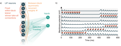
Figure 6: a) RSNN network diagram. The neurons are split into blocks of equal length (here $L=4$) with WTA connectivity between all neurons in the same block. The between-block weights $\mathbf{W}$ are programmed to embed the desired DFA in the RSNN dynamics. The connectivity from each input $s$ is set according to its binary hypervector $\mathbf{\bm{s}}$. b) Membrane potential traces $u_{i}(t)$ of the first 8 neurons within an RSNN. Whenever a neuron spikes (red dots), all neurons within the same block are forced into a refractory state. Thus only the neuron with the greatest postsynaptic current spikes, realising an $\mathrm{argmax}$ function in each block and confining the neural activity to sparse block codes. Between 200ms and 400ms, the second block is masked by an input (either $s_{0}$ or $s_{1}$), which causes the network to switch between attractor states.

The neuron equations were simulated in the Brian 2 SNN simulator [95], using the Euler ODE solver with a default time step of 0,05ms. The weight matrix to embed the chosen DFA was constructed as described in Methods, with $N=2048$ neurons and blocks of length $L=8$. These ideal weights were transformed to binary values, to match that biological synapses may, and neuromorphic synapses often do have very few bits of precision. This binarisation was performed stochastically, via

$$w_{ij}^{\text{binary}}=\begin{cases}1\>\>\text{w.p.}\>\>(1+\exp[-\beta(w_{ij}-\langle w\rangle)/\sigma_{w}])^{-1}\\ 0\>\>\text{otherwise}\end{cases}$$ (11)

where $\langle w\rangle$ and $\sigma_{w}$ are the mean and standard deviation of the ideal weight values respectively, and the steepness parameter $\beta$ is heuristically set to $\beta=2$. This is a common way to embed analog values into binary-valued memristive devices [96]. We then add noise to each weight value, to emulate that the distribution of the binary weight states may themselves be imperfect and even overlapping. The non-ideal weights used in simulation are then given by

$$w_{ij}^{\text{nonideal}}=|w_{ij}^{\text{binary}}+\chi_{ij}|$$ (12)

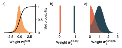
Figure S1: Histograms of the recurrent weight values in simulation before and after nonidealities are applied. a) The ideal weights are shown in yellow, with a sigmoidal transfer function overlain. b) The ideal weights are stochastically binarised according to the sigmoidal set probability. c) The weights after independent Gaussian noise is added to each binarised weight value. The two histograms were each normalised to unit height. These non-idealities emulate that the synaptic weights are imprecise, unreliable and noisy. The weights $w_{ij}^{\text{nonideal}}$ were used in the RSNN in Figure 2.

where $\chi_{ij}$ are independent samples from a centered Gaussian distribution with standard deviation $0.5$. Histograms of the ideal; binary; and non-ideal weights are shown in Figure S1. It is well known that attractor networks are robust to such nonidealities, and that their effect is to reduce the number of attractors that can be reliably stored [10, 97, 98, 28].

The RSNN is initialised in the $q_{0}$ state, and then a sequence of inputs $s_{0}$ or $s_{1}$ are given to the network for 200ms at a time, with gaps in-between. We used this particular timing scheme for simplicity, but the proper functioning of the RSNN is not dependent upon the exact timing of inputs. Each input (and gap) may be given for arbitrarily long periods (Figure S5), needing only to be longer than the attractor-switching time, which is of the order $\tau_{\text{syn}}$.

The firing rate of each attractor state $q$ is given by the dot product of its hypervector $\mathbf{\bm{q}}$ and the vector of kernel-filtered spike activity, i.e.

$$\begin{split}m_{q}(t)=\frac{1}{M}\sum_{i=1}^{N}[\mathbf{\bm{q}}]_{i}\big{(}K(t)\circledast\sum_{\text{spks }k}\delta(t-t_{i}^{k})\big{)}(t)\end{split}$$ (13)

where $m_{q}(t)$ is the firing rate of state $q$, and $K(t)$ is a normalised alpha kernel with time constant $\tau_{\text{readout}}$. If the RSNN is exactly representing a state $q$, then $\langle m_{q}\rangle=\langle\nu\rangle$ where $\langle\nu\rangle$ is the average firing rate of the active neurons. Since the $\mathbf{\bm{q}}$ states are not orthogonal, the expected firing rate of the other $q^{\prime}\neq q$ attractor states $\langle m_{q^{\prime}}\rangle=\langle\nu\rangle/L$ is nonzero. The firing rates of the bridge states $\mathbf{\bm{b}}$ are likewise calculated.

IV-G RRAM crossbar experiment details

The neuron equations were simulated in Python using Euler’s method with the NumPy package. At each time step, if one or multiple neurons spiked, the memristive crossbar was read, and the measured currents were linearly scaled then applied to the postsynaptic neurons in simulation. The experimental measurements were made using non-volatile 1T1R HfO_x-based RRAM chips integrating 32$\times$128 devices. The hardware setup is shown in Figure 3. An FPGA board in the measurement system supports the parallel operation of the WLs, BLs, and SLs of the RRAM chip.

With the 4096 RRAM devices, we could create a fully-connected RSNN with 64 neurons. In simulation and on Loihi, the dimensionality was large enough that we could rely upon the pseudo-orthogonality of randomly-generated hypervector representations. This is not reliably achieved for $N=64$, and so we instead manually chose our sparse block code hypervectors $\mathbf{\bm{q}}$ and $\mathbf{\bm{b}}$ to be orthogonal. The ideal weight matrix $\mathbf{W}$ was constructed as described in Methods, but with the $f$ terms set to $f=0$, to compensate for the fact that our attractor state vectors now have exactly 0 inner product. Since the RRAM devices supported ternary weight states (normalised to $0,0.5,1$), we mapped the ideal weights to ternary weights by applying two thresholds on either side of 0. The distributions of these ternary conductance states are shown in Figure 4.

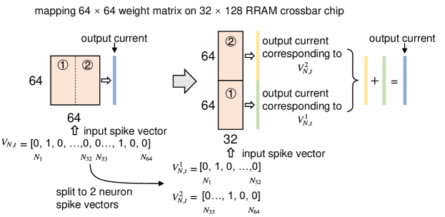
Figure S6: The scheme to map the 64$\times$64 weight matrix to the 32$\times$128 RRAM crossbar chip. We split the size 64 neuron spike vector into two size 32 vectors. We then apply each vector separately as input to the RRAM crossbar one after the other, and read the output currents as depicted. The sum of the two size 64 output current vectors is equivalent to applying a size 64 spike vector as input to a 64$\times$64 crossbar array (shown left). The summation of the two output current vectors is performed in software, and then fed back into the RSNN simulation as postsynaptic currents.

To store the 64$\times$64 weight matrix on the physical RRAM chip, we partitioned it into two 32$\times$64 matrices, and then stored their concatenation on the available 32$\times$128 devices (Figure S6). To perform a current readout (whenever a neuron spiked), we input the binary vector of the first 32 neurons as a voltage via the DACs in parallel, and read the first 64 currents. Then, we input the binary vector of the latter 32 neurons’ spike activity, and added the two current vectors together on the PC. Therefore all but the last multiply-and-accumulate step was performed in-memory.

IV-H Loihi implementation

The experiments were run on the Intel Loihi 2 Oheo Gulch research system using 1024 neurons (128 blocks of 8 neurons) on 95 neurocores. The code was written in Python using Intel’s Lava package.

The network uses the regular current-based leaky integrate and fire neuron model on Loihi. However, different from the hard-coded model, each neuron has a conventional integrative synapse, with weights set by $\mathbf{W}$, and a shunting inhibitory synapse to implement the block-WTA and masking behaviour. To achieve the shunting inhibition synapse, we implemented the neuron using custom neuron microcode, a novel feature of Loihi 2. The microcode on Loihi 2 allows arbitrary instructions from a limited instruction set. To avoid having to create a neuron with 2 registers to store the input, we discriminate the integrative synapse’s input and the shunting synapse’s input by different weight ranges. The shunting synapse’s weight was set to -2048, a value that is never reached by integrating regular input. So, in the microcode, before the regular neuron behaviour is computed, a comparison is made if the input value is below 1000. If it is, the membrane potential is reset to 0 (shunting) and 2048 is added to the input in order not to interfere with the integrative synapse.

The weight matrix was constructed as described in Section IV, and then quantized by linearly mapping the 4-sigma range of $\mathbf{W}$ to the available even integer weight values in the interval $[-254,254]$. These recurrent weights were then written to the all-to-all recurrent synapse weights. Attractor transitions were triggered by stimulating the shunting inhibition synapses, with the input vectors $\mathbf{\bm{s}}_{0}$ or $\mathbf{\bm{s}}_{1}$ to input a 0 or 1, respectively. At the start of the experiment, the RSNN is initialised in the first attractor state $q_{0}$. Inputs are then given for 200 time steps each, with a 200 time step gap in-between, wherein no input is given.

References

Author contributions

M.C. conceived the initial algorithm and its SNN implementation. H.G., A.R. implemented the algorithm on Loihi. H.W. supervised, and J.C., M.C., implemented the algorithm on the memristive crossbar setup. E.N., H.W., G.I., M.Z., E.C. supervised the experiments. All authors contributed to writing the manuscript.

Competing interests

The authors declare no competing interests.

Supplementary Material

S1 Energy function

We can split the neural state vector $\mathbf{\bm{z}}_{t}\in\{0,1\}^{N}$ at time step $t$ into the vector describing only the components in the block, $\mathbf{\bm{z}}^{b}_{t}$, and the vector describing all the other $N-L$ components $\mathbf{\bm{z}}^{\neg b}_{t}$, with $\mathbf{\bm{z}}_{t}=\mathbf{\bm{z}}^{b}_{t}+\mathbf{\bm{z}}^{\neg b}_{t}$. If we define the energy$E_{t}$ at time step $t$ as $E_{t}=-\frac{1}{2}\mathbf{\bm{z}}_{t}^{\intercal}\mathbf{W}\mathbf{\bm{z}}_{t}$, then the change in energy $\Delta E_{t+1}=E_{t+1}-E_{t}$ is given by

$$\Delta E_{t+1}=-(\mathbf{\bm{z}}_{t+1}^{b}-\mathbf{\bm{z}}_{t}^{b})^{\intercal}\mathbf{W}\mathbf{\bm{z}}_{t}^{\neg b}$$ (1)

where we have used that $\mathbf{W}$ is symmetric, and there are no interactions (weight is 0) between neurons in the same block [87]. Now, the block-WTA dynamics mean that each block effectively computes an $\mathrm{argmax}$ over its inputs, meaning that $\mathbf{\bm{z}}_{t+1}^{b}$ maximises the inner product $\mathbf{\bm{z}}_{t+1}^{b\intercal}\mathbf{W}\mathbf{\bm{z}}_{t}^{\neg b}$, and so is the maximum possible value that $\mathbf{\bm{z}}_{t}^{b\intercal}\mathbf{W}\mathbf{\bm{z}}_{t}^{\neg b}$ can take. Thus, we have $\Delta E_{t}\leq 0$, i.e. the network dynamics descend the energy surface $E(\mathbf{\bm{z}})$, which we have constructed to consist of energy wells at our DFA states $\mathbf{\bm{q}}$.

S2 Postsynaptic sum calculations

We first calculate the mean and variance of the components of the postsynaptic sum $\mathbf{\bm{h}}$, in the case that the network is already in state $\mathbf{\bm{q}}^{\mu}\in Q$, and there is no input. We calculate the contribution to $\mathbf{\bm{h}}$ due to the three superimposed matrices in $\mathbf{W}$ separately, for the sake of cleanliness. We will assume that the inner products between different hypervectors are independent (while they are actually only pairwise independent), such that their variances combine linearly.

$$\begin{split}[\mathbf{W}_{\text{attr.}}\mathbf{\bm{q}}^{\mu}]_{i}&=\sum_{\nu}^{Q}(q_{i}^{\nu}-f)(\mathbf{\bm{q}}^{\nu}-f)\cdot\mathbf{\bm{q}}^{\mu}\\ &=M(1-f)(q_{i}^{\mu}-f)+\sum_{\nu\neq\mu}^{Q}\underbrace{(q_{i}^{\nu}-f)}_{\begin{subarray}{c}\text{Mean = 0}\\ \text{Var. = }f(1-f)\end{subarray}}\underbrace{(\mathbf{\bm{q}}^{\nu}-f)\cdot\mathbf{\bm{q}}^{\mu}}_{\begin{subarray}{c}\text{Mean = 0}\\ \text{Var. = }Mf(1-f)\end{subarray}}\\ &=M(1-f)(q_{i}^{\mu}-f)\pm f(1-f)\sqrt{(Q-1)M}\\ &\approx M(q_{i}^{\mu}-f)\pm f\sqrt{MQ}\end{split}$$ (2)

where we are abusing notation somewhat by using $Q$ to denote the number of states in the set $Q$ (and will do the same with $E$ and $S$), and on the last line we make the approximation that $Q\gg 1$ (there are many many DFA states) and $f\ll 1$ (our states are sparse). The corresponding calculation for the bridge matrix is

$$\begin{split}[\mathbf{W}_{\text{brdg.}}\mathbf{\bm{q}}^{\mu}]_{i}&=\sum_{\nu}^{Q}\Big{[}\underbrace{(q_{i}^{\nu}-f)}_{\begin{subarray}{c}\text{Mean = 0}\\ \text{Var. = }f(1-f)\end{subarray}}\underbrace{(\mathbf{\bm{b}}^{\nu}-f)\cdot\mathbf{\bm{q}}^{\mu}}_{\begin{subarray}{c}\text{Mean = 0}\\ \text{Var. = }Mf(1-f)\end{subarray}}+\sum_{s}^{S}\underbrace{(b_{i}^{\nu}-q_{i}^{\nu})}_{\begin{subarray}{c}\text{Mean = 0}\\ \text{Var. = }2f(1-f)\end{subarray}}\underbrace{((\mathbf{\bm{b}}^{\nu}-f)\circ\overline{\mathbf{\bm{s}}})\cdot\mathbf{\bm{q}}^{\mu}}_{\begin{subarray}{c}\text{Mean = 0}\\ \text{Var. = }Mf(1-f)\end{subarray}}\Big{]}\\ &=0\pm f(1-f)\sqrt{MQ(1+2S)}\\ &\approx 0\pm f\sqrt{MQ(1+2S)}\\ \end{split}$$ (3)

If we are constructing a DFA with many inputs (large $S$), but each state has incoming edges with only a few of these inputs, then the capacity of the network can be increased by here summing not over all inputs, but only over the unique inputs of the edges to the state $q$. The transition matrix calculation goes

$$\begin{split}[\mathbf{W}_{\text{tran.}}\mathbf{\bm{q}}^{\mu}]_{i}&=\sum_{\eta}^{E}(b_{i}^{\prime}-q_{i})((\mathbf{\bm{q}}-f)\circ\overline{\mathbf{\bm{s}}})\cdot\mathbf{\bm{q}}^{\mu}\\ &=\sum_{\eta|q\neq q^{\mu}}^{E}\underbrace{(b_{i}^{\prime}-q_{i})}_{\begin{subarray}{c}\text{Mean = 0}\\ \text{Var. = }2f(1-f)\end{subarray}}\underbrace{((\mathbf{\bm{q}}-f)\circ\overline{\mathbf{\bm{s}}})\cdot\mathbf{\bm{q}}^{\mu}}_{\begin{subarray}{c}\text{Mean = 0}\\ \text{Var. = }Mf(1-f)\end{subarray}}+\sum_{\eta|q=q^{\mu}}^{E}\underbrace{(b_{i}^{\prime}-q_{i})}_{\begin{subarray}{c}\text{Mean = 0}\\ \text{Var. = }2f(1-f)\end{subarray}}\underbrace{((\mathbf{\bm{q}}^{\mu}-f)\circ\overline{\mathbf{\bm{s}}})\cdot\mathbf{\bm{q}}^{\mu}}_{\begin{subarray}{c}\text{Mean = 0}\\ \text{Var. = }M(1-f)^{2}\end{subarray}}\\ &=0\pm(1-f)\sqrt{2Mf^{2}(E-S)+2MSf(1-f)}\\ &\approx 0\pm\sqrt{2Mf^{2}E+2MSf}\\ \end{split}$$ (4)

where we split the summation up into transitions whose source state is $q^{\mu}$ (and those with a different source state). We then assume the worse-case scenario that $S$ of the $E$ edges have $q^{\mu}$ as a source state. The final postsynaptic sum is given by

$$\begin{split}[\mathbf{\bm{h}}]_{i}=[\mathbf{W}\mathbf{\bm{q}}^{\mu}]_{i}&\approx M(q_{i}^{\mu}-f)\pm\sqrt{M}\sqrt{2f^{2}Q(1+S)+2f^{2}E+2fS}\\ &\propto q_{i}^{\mu}-f\pm\sqrt{\frac{2}{N}}\sqrt{fQ(1+S)+fE+S}\\ \end{split}$$ (5)

from which we get $\langle\mathbf{W}\mathbf{\bm{q}}^{\mu}\rangle\propto\mathbf{\bm{q}}^{\mu}-f$.

We then calculate the postsynaptic sum when we are masking the network with an input $s^{\lambda}$, and we assume there exists an edge $\epsilon\in E$ with source state $q^{\mu}$ and input $s^{\lambda}$. Calculating $\mathbf{\bm{h}}$ in the same way, we have

$$\begin{split}[\mathbf{W}_{\text{attr.}}(\mathbf{\bm{q}}^{\mu}\land\mathbf{\bm{s}}^{\lambda})]_{i}&=\sum_{\nu}^{Q}(q_{i}^{\nu}-f)(\mathbf{\bm{q}}^{\nu}-f)\cdot(\mathbf{\bm{q}}^{\mu}\land\mathbf{\bm{s}}^{\lambda})\\ &=\frac{1}{2}M(1-f)(q_{i}^{\mu}-f)+\sum_{\nu\neq\mu}^{Q}\underbrace{(q_{i}^{\nu}-f)}_{\begin{subarray}{c}\text{Mean = 0}\\ \text{Var. = }f(1-f)\end{subarray}}\underbrace{(\mathbf{\bm{q}}^{\nu}-f)\cdot(\mathbf{\bm{q}}^{\mu}\land\mathbf{\bm{s}}^{\lambda})}_{\begin{subarray}{c}\text{Mean = 0}\\ \text{Var. = }\frac{1}{2}Mf(1-f)\end{subarray}}\\ &=\frac{1}{2}M(1-f)(q_{i}^{\mu}-f)\pm f(1-f)\sqrt{(Q-1)\frac{1}{2}M}\\ &\approx\frac{1}{2}M(q_{i}^{\mu}-f)\pm f\sqrt{\frac{1}{2}MQ}\end{split}$$ (6)

and for the bridge matrix

$$\begin{split}[\mathbf{W}_{\text{brdg.}}(\mathbf{\bm{q}}^{\mu}\land\mathbf{\bm{s}}^{\lambda})]_{i}&=\sum_{\nu}^{Q}\Big{[}\underbrace{(q_{i}^{\nu}-f)}_{\begin{subarray}{c}\text{Mean = 0}\\ \text{Var. = }f(1-f)\end{subarray}}\underbrace{(\mathbf{\bm{b}}^{\nu}-f)\cdot(\mathbf{\bm{q}}^{\mu}\land\mathbf{\bm{s}}^{\lambda})}_{\begin{subarray}{c}\text{Mean = 0}\\ \text{Var. = }\frac{1}{2}Mf(1-f)\end{subarray}}+\sum_{s}^{S}\underbrace{(b_{i}^{\nu}-q_{i}^{\nu})}_{\begin{subarray}{c}\text{Mean = 0}\\ \text{Var. = }2f(1-f)\end{subarray}}\underbrace{((\mathbf{\bm{b}}^{\nu}-f)\circ\overline{\mathbf{\bm{s}}})\cdot(\mathbf{\bm{q}}^{\mu}\land\mathbf{\bm{s}}^{\lambda})}_{\begin{subarray}{c}\text{Mean = 0}\\ \text{Var. = }\frac{1}{2}Mf(1-f)\end{subarray}}\Big{]}\\ &=0\pm f(1-f)\sqrt{\frac{1}{2}MQ(1+2S)}\\ &\approx 0\pm f\sqrt{\frac{1}{2}MQ(1+2S)}\\ \end{split}$$ (7)

and the transition matrix

$$\begin{split}&[\mathbf{W}_{\text{tran.}}(\mathbf{\bm{q}}^{\mu}\land\mathbf{\bm{s}}^{\lambda})]_{i}=\sum_{\eta}^{E}(b_{i}^{\prime}-q_{i})((\mathbf{\bm{q}}-f)\circ\overline{\mathbf{\bm{s}}})\cdot(\mathbf{\bm{q}}^{\mu}\land\mathbf{\bm{s}}^{\lambda})\\ &=(1-f)\frac{M}{2}(b_{i}^{\prime}-q_{i}^{\mu})+\sum_{\begin{subarray}{c}\eta\neq\epsilon\\ \text{and }q\neq q^{\mu}\end{subarray}}^{E}\underbrace{(b_{i}^{\prime}-q_{i})}_{\begin{subarray}{c}\text{Mean = 0}\\ \text{Var. = }2f(1-f)\end{subarray}}\underbrace{((\mathbf{\bm{q}}-f)\circ\overline{\mathbf{\bm{s}}})\cdot(\mathbf{\bm{q}}^{\mu}\land\mathbf{\bm{s}}^{\lambda})}_{\begin{subarray}{c}\text{Mean = 0}\\ \text{Var. = }\frac{M}{2}f(1-f)\end{subarray}}+\sum_{\begin{subarray}{c}\eta\neq\epsilon\\ \text{and }q=q^{\mu}\end{subarray}}^{E}\underbrace{(b_{i}^{\prime}-q_{i})}_{\begin{subarray}{c}\text{Mean = 0}\\ \text{Var. = }2f(1-f)\end{subarray}}\underbrace{((\mathbf{\bm{q}}-f)\circ\overline{\mathbf{\bm{s}}})\cdot(\mathbf{\bm{q}}^{\mu}\land\mathbf{\bm{s}}^{\lambda})}_{\begin{subarray}{c}\text{Mean = 0}\\ \text{Var. = }\frac{M}{2}(1-f)^{2}\end{subarray}}\\ &=\frac{1}{2}M(1-f)(b_{i}^{\prime}-q_{i}^{\mu})\pm(1-f)\sqrt{M\big{(}f^{2}(E-S+1)+(S-1)f(1-f)\big{)}}\\ &\approx\frac{1}{2}M(b_{i}^{\prime}-q_{i}^{\mu})\pm\sqrt{M(f^{2}E+f(S-1))}\end{split}$$ (8)

where we split the summation over all transitions $E$ into the correct transition $\epsilon$, incorrect transitions with different source states, and incorrect transitions with the same source state. We then assume the worst case that there are $S-1$ incorrect transitions with the same source state.

Combining the three again, we get

$$\begin{split}[\mathbf{\bm{h}}]_{i}=[\mathbf{W}(\mathbf{\bm{q}}^{\mu}\land\mathbf{\bm{s}}^{\lambda})]_{i}&\approx\frac{M}{2}(b_{i}^{\prime}-f)\pm\sqrt{M}\sqrt{f^{2}Q(1+S)+f^{2}E+f(S-1)}\\ &\propto(b_{i}^{\prime}-f)\pm\frac{2}{\sqrt{N}}\sqrt{fQ(1+S)+fE+S-1}\end{split}$$ (9)

which in expectation gives us $\langle\mathbf{W}(\mathbf{\bm{q}}^{\mu}\land\mathbf{\bm{s}}^{\lambda})\rangle\propto\mathbf{\bm{b}}^{\prime}-f$. The same procedure can be applied to calculate the mean and variance of the postsynaptic sum in all cases.

S3 Sparse block code representational capacity

We here derive a result, adapted from [32], that the number of sparse block code (SBC) hypervectors that can be randomly-generated without accidentally incurring a significant degree of overlap between any pair of them, is exponential in dimension $N$, and so very large for reasonable values of $N$ and $L$.

We generate SBC hypervectors of dimension $N$, with block length $L$, and number of blocks $M=N/L$. The coding level is then $f=1/L$. The normalised similarity between SBC hypervectors is given by

$$\mathrm{sim}(\mathbf{\bm{a}},\mathbf{\bm{b}})=\frac{1}{M}\mathbf{\bm{a}}\cdot\mathbf{\bm{b}}$$ (10)

such that the the similarity between identical hypervectors $\mathrm{sim}(\mathbf{\bm{a}},\mathbf{\bm{a}})=1$, and the expected similarity between independent hypervectors is $\langle\mathrm{sim}(\mathbf{\bm{a}},\mathbf{\bm{b}})\rangle=f<1$.

We first provide a bound on the similarity between independent hypervectors. We can rewrite the similarity between SBC hypervectors as

$$\mathrm{sim}(\mathbf{\bm{a}},\mathbf{\bm{b}})=\frac{1}{M}\sum_{i=1}^{M}X_{i}$$ (11)

where $X_{i}\in\{0,1\}$ denotes whether the same neuron in the $i$’th block is active in both hypervectors, with $\langle X_{i}\rangle=f$. By Hoeffding’s inequality, this sum is bounded by

$$\mathbb{P}\big{[}\mathrm{sim}(\mathbf{\bm{a}},\mathbf{\bm{b}})-f\geq\theta\big{]}\leq\exp\big{(}-2M\theta^{2}\big{)}$$ (12)

where $\theta$ is a threshold of our choosing. This bound gives us assurances about how much the similarity between independent hypervectors can deviate from the expected value $f$. We can then set $\theta$ to represent the maximum acceptable similarity between independent hypervectors. Given that independent hypervectors have expected similarity $f$, and identical hypervectors have similarity $1$, then a reasonable threshold might halfway between them, $\theta=\frac{1}{2}(1-f)$. For reasonable values of $N=1000$, $L=8$, the probability that a given pair of independent hypervectors exceeds $\theta$ is then less than $10^{-20}$.

We however want a bound on the number $K$ of SBC hypervectors that can be generated, for which none of the possible inner product pairs exceed $\theta$. For $K$ hypervectors, there are $\frac{1}{2}K(K-1)<\frac{1}{2}K^{2}$ pairs to check. By Boole’s inequality, that the union probability of a set of events occurring $\mathbb{P}\big{[}\bigcup_{i}E_{i}\big{]}\leq\sum_{i}\mathbb{P}[E_{i}]$ for some countable events $\{E_{i}\}$ (whether a similarity exceeds $\theta$), we have

$$\mathbb{P}[\text{any pair exceeds $\theta$}]\leq\delta=\sum_{j=1}^{\frac{1}{2}K^{2}}\exp\big{(}-2M\theta^{2}\big{)}=\frac{1}{2}K^{2}\exp\big{(}-2M\theta^{2}\big{)}$$ (13)

where we have introduced $\delta\in[0,1]$ as the acceptable probability of a collision, which we will set to $\delta\ll 1$. We can then rearrange for the number of hypervectors $K$,

$$K=\sqrt{2\delta}\exp\Big{(}M\theta^{2}\Big{)}=\sqrt{2\delta}\exp\Big{(}N\theta^{2}/L\Big{)}$$ (14)

and so the number of SBC hypervectors that can be generated before a collision becomes likely, is exponential in dimension $N$. For comparison, the number of orthogonal localist representations that can be generated is linear in $N$.

For reasonable values of $N=1000$, $L=8$, with an acceptable failure probability of $\delta=0.0001$, then with probability greater than $0.9999$, we can generate $K\approx 3\times 10^{9}$ SBC hypervectors before a collision occurs, which is well in excess of the number of states that can be stored in an attractor network, which scales at most with the number of synapses $N^{2}$.

Parameter	Description	First simulation	Crossbar experiment	Big simulation	Loihi
$N$	Number of neurons	2048	64	2048	1024
$L$	Block length	8	8	16	8
$\langle|w_{ij}|\rangle$	Synaptic weight strength	$\approx\qty{0.1}{\milli\per}$	$\approx\qty{4}{\milli\per}$	$\approx\qty{0,2}{\milli\per}$	$\approx 45$
$C$	Membrane capacitance	1F	1F	1F	-
$\tau_{m}$	Membrane time constant	20ms	20ms	20ms	10
$u_{\theta}$	Spiking threshold	20mV	20mV	20mV	1000
$u_{\text{rest}}$	Resting potential	25mV	25mV	25mV	0
$u_{\text{reset}}$	Reset potential	0mV	0mV	0mV	0
$\tau_{\text{syn}}$	Synaptic time constant	20ms	20ms	20ms	-
$\tau_{\text{ref}}$	Refractory period	10ms	10ms	10ms	0
$\tau_{\text{readout}}$	Readout kernel timescale	10ms	10ms	10ms	10

TABLE I: Parameters used in the simulation, closed-loop memristive crossbar and Loihi setups. The magnitude of the synaptic weights $\langle|w_{ij}|\rangle$ is the total amount of charge that each spike adds to a postsynaptic neuron’s membrane.

References

- [1] C. Mead “Neuromorphic electronic systems” Conference Name: Proceedings of the IEEE In Proceedings of the IEEE 78.10, 1990, pp. 1629–1636 DOI: 10.1109/5.58356
- [2] Surya Ganguli, Dongsung Huh and Haim Sompolinsky “Memory traces in dynamical systems” In Proceedings of the National Academy of Sciences 105.48 National Academy of Sciences, 2008, pp. 18970–18975 DOI: 10.1073/pnas.0804451105
- [3] Mikail Khona and Ila R. Fiete “Attractor and integrator networks in the brain” Number: 12 Publisher: Nature Publishing Group In Nature Reviews Neuroscience 23.12, 2022, pp. 744–766 DOI: 10.1038/s41583-022-00642-0
- [4] Sepp Hochreiter and Jürgen Schmidhuber “Long short-term memory” In Neural Computation 9.8, 1997, pp. 1735–1780 DOI: 10.1162/neco.1997.9.8.1735
- [5] Guillaume Bellec et al. “A solution to the learning dilemma for recurrent networks of spiking neurons” Number: 1 Publisher: Nature Publishing Group In Nature Communications 11.1, 2020, pp. 3625 DOI: 10.1038/s41467-020-17236-y
- [6] Benjamin Cramer et al. “Surrogate gradients for analog neuromorphic computing” Publisher: Proceedings of the National Academy of Sciences In Proceedings of the National Academy of Sciences 119.4, 2022, pp. e2109194119 DOI: 10.1073/pnas.2109194119
- [7] Emre O. Neftci, Hesham Mostafa and Friedemann Zenke “Surrogate gradient learning in spiking neural networks” arXiv:1901.09948 [cs, q-bio] arXiv, 2019 DOI: 10.48550/arXiv.1901.09948
- [8] John Miller and Moritz Hardt “Stable recurrent models” In International Conference on Learning Representations, 2019 URL: https://openreview.net/forum?id=Hygxb2CqKm
- [9] J.. Hopfield “Neural networks and physical systems with emergent collective computational abilities” Publisher: National Academy of Sciences Section: Research Article In Proceedings of the National Academy of Sciences 79.8, 1982, pp. 2554–2558 DOI: 10.1073/pnas.79.8.2554
- [10] Daniel J. Amit “Modeling brain function: the world of attractor neural networks, 1st edition”, 1989 DOI: 10.1017/CBO9780511623257
- [11] Thomas Bohnstingl et al. “Biologically-inspired training of spiking recurrent neural networks with neuromorphic hardware” In 2022 IEEE 4th International Conference on Artificial Intelligence Circuits and Systems (AICAS), 2022, pp. 218–221 DOI: 10.1109/AICAS54282.2022.9869963
- [12] Sebastian Schmitt et al. “Neuromorphic hardware in the loop: Training a deep spiking network on the BrainScaleS wafer-scale system” ISSN: 2161-4407 In 2017 International Joint Conference on Neural Networks (IJCNN), 2017, pp. 2227–2234 DOI: 10.1109/IJCNN.2017.7966125
- [13] Yigit Demirag, Charlotte Frenkel, Melika Payvand and Giacomo Indiveri “Online training of spiking recurrent neural networks with phase-change memory synapses” arXiv:2108.01804 [cs] arXiv, 2021 DOI: 10.48550/arXiv.2108.01804
- [14] Uğurcan Çakal et al. “Gradient-descent hardware-aware training and deployment for mixed-signal Neuromorphic processors” arXiv:2303.12167 [cs] arXiv, 2024 DOI: 10.48550/arXiv.2303.12167
- [15] Denis Kleyko et al. “Vector symbolic architectures as a computing framework for emerging hardware” Conference Name: Proceedings of the IEEE In Proceedings of the IEEE 110.10, 2022, pp. 1538–1571 DOI: 10.1109/JPROC.2022.3209104
- [16] Denis Kleyko, Dmitri A. Rachkovskij, Evgeny Osipov and Abbas Rahimi “A survey on hyperdimensional computing aka vector symbolic architectures, part I: Models and data transformations” In ACM Computing Surveys 55.6, 2022, pp. 130:1–130:40 DOI: 10.1145/3538531
- [17] Pentti Kanerva “Hyperdimensional computing: An introduction to computing in distributed representation with high-dimensional random vectors” In Cognitive Computation 1.2, 2009, pp. 139–159 DOI: 10.1007/s12559-009-9009-8
- [18] T.. Plate “Holographic reduced representations” Conference Name: IEEE Transactions on Neural Networks In IEEE Transactions on Neural Networks 6.3, 1995, pp. 623–641 DOI: 10.1109/72.377968
- [19] Ross W. Gayler “Multiplicative binding, representation operators & analogy” In Advances in Analogy Research: Integration of Theory and Data from the Cognitive, Computational, and Neural Sciences, 1998 URL: http://cogprints.org/502/
- [20] Geethan Karunaratne et al. “In-memory hyperdimensional computing” Bandiera_abtest: a Cg_type: Nature Research Journals Number: 6 Primary_atype: Research Publisher: Nature Publishing Group Subject_term: Computer science;Electronic devices Subject_term_id: computer-science;electronic-devices In Nature Electronics 3.6, 2020, pp. 327–337 DOI: 10.1038/s41928-020-0410-3
- [21] Madison Cotteret, Hugh Greatorex, Martin Ziegler and Elisabetta Chicca “Vector symbolic finite state machines in attractor neural networks” In Neural Computation 36.4, 2024, pp. 549–595 DOI: 10.1162/neco˙a˙01638
- [22] E. Neftci et al. “Synthesizing cognition in neuromorphic electronic systems” In Proceedings of the National Academy of Sciences 110.37, 2013, pp. E3468–E3476 DOI: 10.1073/pnas.1212083110
- [23] Dongchen Liang and Giacomo Indiveri “A neuromorphic computational primitive for robust context-dependent decision making and context-dependent stochastic computation” Conference Name: IEEE Transactions on Circuits and Systems II: Express Briefs In IEEE Transactions on Circuits and Systems II: Express Briefs 66.5, 2019, pp. 843–847 DOI: 10.1109/TCSII.2019.2907848
- [24] Garrick Orchard et al. “Efficient neuromorphic signal processing with Loihi 2” arXiv:2111.03746 [cs] arXiv, 2021 DOI: 10.48550/arXiv.2111.03746
- [25] Peter Dayan “Simple substrates for complex cognition” In Frontiers in Neuroscience 2, 2008, pp. 31 DOI: 10.3389/neuro.01.031.2008
- [26] Mika Laiho, Jussi H. Poikonen, Pentti Kanerva and Eero Lehtonen “High-dimensional computing with sparse vectors” In 2015 IEEE Biomedical Circuits and Systems Conference (BioCAS), 2015, pp. 1–4 DOI: 10.1109/BioCAS.2015.7348414
- [27] Edward Paxon Frady, Denis Kleyko and Friedrich T. Sommer “Variable binding for sparse distributed representations: Theory and applications” Conference Name: IEEE Transactions on Neural Networks and Learning Systems In IEEE Transactions on Neural Networks and Learning Systems 34.5, 2023, pp. 2191–2204 DOI: 10.1109/TNNLS.2021.3105949
- [28] Andreas Knoblauch, Günther Palm and Friedrich T. Sommer “Memory capacities for synaptic and structural plasticity” In Neural Computation 22.2, 2010, pp. 289–341 DOI: 10.1162/neco.2009.08-07-588
- [29] Shun-ichi Amari “Characteristics of sparsely encoded associative memory” In Neural Networks 2.6, 1989, pp. 451–457 DOI: 10.1016/0893-6080(89)90043-9
- [30] M.. Tsodyks and M.. Feigel’man “The enhanced storage capacity in neural networks with low activity level” Publisher: IOP Publishing In Europhysics Letters (EPL) 6.2, 1988, pp. 101–105 DOI: 10.1209/0295-5075/6/2/002
- [31] D.. Rumelhart and J.. McClelland “Parallel distributed processing: explorations in the microstructure of cognition. Volume 1. Foundations” Publisher: MIT Press,Cambridge, MA, 1986 URL: https://www.osti.gov/biblio/5838709
- [32] Anthony Thomas, Sanjoy Dasgupta and Tajana Rosing “A theoretical perspective on hyperdimensional computing” In Journal of Artificial Intelligence Research 72, 2022, pp. 215–249 DOI: 10.1613/jair.1.12664
- [33] Günther Palm “Neural associative memories and sparse coding” In Neural Networks 37, Twenty-fifth Anniversay Commemorative Issue, 2013, pp. 165–171 DOI: 10.1016/j.neunet.2012.08.013
- [34] Christopher J. Rozell, Don H. Johnson, Richard G. Baraniuk and Bruno A. Olshausen “Sparse coding via thresholding and local competition in neural circuits” In Neural Computation 20.10, 2008, pp. 2526–2563 DOI: 10.1162/neco.2008.03-07-486
- [35] Emre Neftci and Giacomo Indiveri “A device mismatch compensation method for VLSI neural networks” ISSN: 2163-4025 In 2010 Biomedical Circuits and Systems Conference (BioCAS), 2010, pp. 262–265 DOI: 10.1109/BIOCAS.2010.5709621
- [36] Julian Büchel et al. “Supervised training of spiking neural networks for robust deployment on mixed-signal neuromorphic processors” Publisher: Nature Publishing Group In Scientific Reports 11.1, 2021, pp. 23376 DOI: 10.1038/s41598-021-02779-x
- [37] Hugh Greatorex et al. “TEXEL: A mixed-signal neuromorphic processor with on-chip learning for beyond-CMOS device integration” In In preparation, 2024
- [38] A. Fantini et al. “Intrinsic program instability in HfO2 RRAM and consequences on program algorithms” In 2015 IEEE International Electron Devices Meeting (IEDM), 2015, pp. 7.5.1–7.5.4 DOI: 10.1109/IEDM.2015.7409648
- [39] Chen Wang et al. “Relaxation Effect in RRAM Arrays: Demonstration and Characteristics” In IEEE Electron Device Letters 37.2, 2016, pp. 182–185 DOI: 10.1109/LED.2015.2508034
- [40] Junren Chen et al. “Scaling limits of memristor-based routers for asynchronous neuromorphic systems” Conference Name: IEEE Transactions on Circuits and Systems II: Express Briefs In IEEE Transactions on Circuits and Systems II: Express Briefs 71.3, 2024, pp. 1576–1580 DOI: 10.1109/TCSII.2023.3343292
- [41] Simone D’Agostino et al. “DenRAM: neuromorphic dendritic architecture with RRAM for efficient temporal processing with delays” Publisher: Nature Publishing Group In Nature Communications 15.1, 2024, pp. 3446 DOI: 10.1038/s41467-024-47764-w
- [42] W.. Little “The existence of persistent states in the brain” In Mathematical Biosciences 19.1, 1974, pp. 101–120 DOI: 10.1016/0025-5564(74)90031-5
- [43] Edmund Rolls “The mechanisms for pattern completion and pattern separation in the hippocampus” In Frontiers in systems neuroscience 7, 2013, pp. 74 DOI: 10.3389/fnsys.2013.00074
- [44] Rishidev Chaudhuri and Ila Fiete “Computational principles of memory” Number: 3 Publisher: Nature Publishing Group In Nature Neuroscience 19.3, 2016, pp. 394–403 DOI: 10.1038/nn.4237
- [45] Elad Schneidman, Michael J. Berry, Ronen Segev and William Bialek “Weak pairwise correlations imply strongly correlated network states in a neural population” In Nature 440.7087, 2006, pp. 1007–1012 DOI: 10.1038/nature04701
- [46] Valerio Mante, David Sussillo, Krishna V. Shenoy and William T. Newsome “Context-dependent computation by recurrent dynamics in prefrontal cortex” Number: 7474 Publisher: Nature Publishing Group In Nature 503.7474, 2013, pp. 78–84 DOI: 10.1038/nature12742
- [47] David Sussillo and Omri Barak “Opening the black box: low-dimensional dynamics in high-dimensional recurrent neural networks” In Neural computation 25.3 MIT Press One Rogers Street, Cambridge, MA 02142-1209, USA journals-info …, 2013, pp. 626–649
- [48] Paul Miller “Itinerancy between attractor states in neural systems” In Current opinion in neurobiology 40, 2016, pp. 14–22 DOI: 10.1016/j.conb.2016.05.005
- [49] Ueli Rutishauser and Rodney Douglas “State-dependent computation using coupled recurrent networks” In Neural computation 21, 2009, pp. 478–509 DOI: 10.1162/neco.2008.03-08-734
- [50] S. Fusi, E. Miller and Mattia Rigotti “Why neurons mix: high dimensionality for higher cognition” In Current Opinion in Neurobiology, 2016 DOI: 10.1016/j.conb.2016.01.010
- [51] Kenneth L. Clarkson, Shashanka Ubaru and Elizabeth Yang “Capacity analysis of vector symbolic architectures” arXiv:2301.10352 [cs] arXiv, 2023 DOI: 10.48550/arXiv.2301.10352
- [52] Hamza Errahmouni Barkam et al. “Reliable hyperdimensional reasoning on unreliable emerging technologies” ISSN: 1558-2434 In 2023 IEEE/ACM International Conference on Computer Aided Design (ICCAD), 2023, pp. 1–9 DOI: 10.1109/ICCAD57390.2023.10323935
- [53] E. Frady and Friedrich T. Sommer “Robust computation with rhythmic spike patterns” Publisher: National Academy of Sciences Section: PNAS Plus In Proceedings of the National Academy of Sciences 116.36, 2019, pp. 18050–18059 DOI: 10.1073/pnas.1902653116
- [54] Alpha Renner et al. “Neuromorphic visual scene understanding with resonator networks” arXiv:2208.12880 [cs, eess] arXiv, 2022 DOI: 10.48550/arXiv.2208.12880
- [55] Zhuowen Zou et al. “Memory-inspired spiking hyperdimensional network for robust online learning” Number: 1 Publisher: Nature Publishing Group In Scientific Reports 12.1, 2022, pp. 7641 DOI: 10.1038/s41598-022-11073-3
- [56] Justin Morris et al. “HyperSpike: Hyperdimensional computing for more efficient and robust spiking neural networks” ISSN: 1558-1101 In 2022 Design, Automation & Test in Europe Conference & Exhibition (DATE), 2022, pp. 664–669 DOI: 10.23919/DATE54114.2022.9774644
- [57] D. Horn and M. Usher “Neural networks with dynamical thresholds” Publisher: American Physical Society In Physical Review A 40.2, 1989, pp. 1036–1044 DOI: 10.1103/PhysRevA.40.1036
- [58] Friedrich T. Sommer and Thomas Wennekers “Synfire chains with conductance-based neurons: internal timing and coordination with timed input” In Neurocomputing 65-66, Computational Neuroscience: Trends in Research 2005, 2005, pp. 449–454 DOI: 10.1016/j.neucom.2004.10.015
- [59] Takeshi Kambara, Yoshiki Kashimori, Noriaki Usuba and Osamu Hoshino “Role of itinerancy among attractors as dynamical map in distributed coding scheme” In Neural Networks: The Official Journal of the International Neural Network Society 10.8, 1997, pp. 1375–1390 DOI: 10.1016/s0893-6080(97)00022-1
- [60] H. Gutfreund and M. Mezard “Processing of temporal sequences in neural networks” Publisher: American Physical Society In Physical Review Letters 61.2, 1988, pp. 235–238 DOI: 10.1103/PhysRevLett.61.235
- [61] Daniel J. Amit “Neural networks counting chimes” Publisher: National Academy of Sciences In Proceedings of the National Academy of Sciences of the United States of America 85.7, 1988, pp. 2141–2145 DOI: 10.1073/pnas.85.7.2141
- [62] Marc F.. Drossaers “Hopfield models as nondeterministic finite-state machines” In Proceedings of the 14th conference on Computational linguistics - Volume 1, COLING ’92 USA: Association for Computational Linguistics, 1992, pp. 113–119 DOI: 10.3115/992066.992087
- [63] Bolun Chen and Paul Miller “Attractor-state itinerancy in neural circuits with synaptic depression” In The Journal of Mathematical Neuroscience 10.1, 2020, pp. 15 DOI: 10.1186/s13408-020-00093-w
- [64] P. Peretto and J.. Niez “Collective properties of neural networks” In Disordered Systems and Biological Organization Berlin, Heidelberg: Springer Berlin Heidelberg, 1986, pp. 171–185
- [65] Evgeny Osipov, Denis Kleyko and Alexander Legalov “Associative synthesis of finite state automata model of a controlled object with hyperdimensional computing” In IECON 2017 - 43rd Annual Conference of the IEEE Industrial Electronics Society, 2017, pp. 3276–3281 DOI: 10.1109/IECON.2017.8216554
- [66] M. Maestro-Izquierdo et al. “Gamma radiation effects on HfO2-based RRAM devices” ISSN: 2643-1300 In 2021 13th Spanish Conference on Electron Devices (CDE), 2021, pp. 23–26 DOI: 10.1109/CDE52135.2021.9455719
- [67] Sandro Baumgartner et al. “Visual pattern recognition with on on-chip learning: towards a fully neuromorphic approach” In 2020 IEEE International Symposium on Circuits and Systems (ISCAS), 2020, pp. 1–5 IEEE
- [68] Denis Kleyko, Dmitri Rachkovskij, Evgeny Osipov and Abbas Rahimi “A survey on hyperdimensional computing aka vector symbolic architectures, part II: Applications, cognitive models, and challenges” In ACM Computing Surveys 55.9, 2023, pp. 175:1–175:52 DOI: 10.1145/3558000
- [69] Peer Neubert, Stefan Schubert and Peter Protzel “An introduction to hyperdimensional computing for robotics” In KI - Künstliche Intelligenz 33.4, 2019, pp. 319–330 DOI: 10.1007/s13218-019-00623-z
- [70] Thomas Yerxa, Alexander Anderson and Eric Weiss “The hyperdimensional stack machine” In Cognitive Computing, 2018, pp. 1–2
- [71] David Marr “Vision: A computational investigation into the human representation and processing of visual information” W. H. FreemanCompany, 1982
- [72] André J. Noest “Phasor neural networks” In Proceedings of the 1987 International Conference on Neural Information Processing Systems, NIPS’87 Cambridge, MA, USA: MIT Press, 1987, pp. 584–591
- [73] Catherine D. Schuman et al. “Opportunities for neuromorphic computing algorithms and applications” Publisher: Nature Publishing Group In Nature Computational Science 2.1, 2022, pp. 10–19 DOI: 10.1038/s43588-021-00184-y
- [74] Herbert Jaeger, Beatriz Noheda and Wilfred G. Wiel “Toward a formal theory for computing machines made out of whatever physics offers” Publisher: Nature Publishing Group In Nature Communications 14.1, 2023, pp. 4911 DOI: 10.1038/s41467-023-40533-1
- [75] Fabio Stefanini, Emre O. Neftci, Sadique Sheik and Giacomo Indiveri “PyNCS: a microkernel for high-level definition and configuration of neuromorphic electronic systems” Publisher: Frontiers In Frontiers in Neuroinformatics 8, 2014 DOI: 10.3389/fninf.2014.00073
- [76] Andrew P. Davison et al. “PyNN: a common interface for neuronal network simulators” Publisher: Frontiers In Frontiers in Neuroinformatics 2, 2009 DOI: 10.3389/neuro.11.011.2008
- [77] James B. Aimone, William Severa and Craig M. Vineyard “Composing neural algorithms with Fugu” arXiv:1905.12130 [cs] arXiv, 2019 DOI: 10.48550/arXiv.1905.12130
- [78] Youhui Zhang et al. “A system hierarchy for brain-inspired computing” Publisher: Nature Publishing Group In Nature 586.7829, 2020, pp. 378–384 DOI: 10.1038/s41586-020-2782-y
- [79] Chris Eliasmith “A unified approach to building and controlling spiking attractor networks” In Neural Computation 17.6, 2005, pp. 1276–1314 DOI: 10.1162/0899766053630332
- [80] Julia Steinberg and Haim Sompolinsky “Associative memory of structured knowledge” Number: 1 Publisher: Nature Publishing Group In Scientific Reports 12.1, 2022, pp. 21808 DOI: 10.1038/s41598-022-25708-y
- [81] V.. Gritsenko et al. “Neural distributed autoassociative memories: a survey” arXiv:1709.00848 [cs] In Kibernetika i vyčislitel’naâ tehnika 2017.2(188), 2017, pp. 5–35 DOI: 10.15407/kvt188.02.005
- [82] E. Frady, Spencer J. Kent, Bruno A. Olshausen and Friedrich T. Sommer “Resonator networks, 1: An efficient solution for factoring high-dimensional, distributed representations of data structures” In Neural Computation 32.12, 2020, pp. 2311–2331 DOI: 10.1162/neco˙a˙01331
- [83] Netanel Raviv “Linear codes for hyperdimensional computing” arXiv:2403.03278 [cs, math] version: 1 arXiv, 2024 DOI: 10.48550/arXiv.2403.03278
- [84] Michael Hersche et al. “A neuro-vector-symbolic architecture for solving Raven’s progressive matrices” Number: 4 Publisher: Nature Publishing Group In Nature Machine Intelligence 5.4, 2023, pp. 363–375 DOI: 10.1038/s42256-023-00630-8
- [85] Tony A. Plate “Analogy retrieval and processing with distributed vector representations” _eprint: https://onlinelibrary.wiley.com/doi/pdf/10.1111/1468-0394.00125 In Expert Systems 17.1, 2000, pp. 29–40 DOI: 10.1111/1468-0394.00125
- [86] Marvin L. Minsky “Computation: finite and infinite machines” USA: Prentice-Hall, Inc., 1967
- [87] Michael A. Cohen and Stephen Grossberg “Absolute stability of global pattern formation and parallel memory storage by competitive neural networks” Conference Name: IEEE Transactions on Systems, Man, and Cybernetics In IEEE Transactions on Systems, Man, and Cybernetics SMC-13.5, 1983, pp. 815–826 DOI: 10.1109/TSMC.1983.6313075
- [88] J. Buhmann and K. Schulten “Noise-driven temporal association in neural networks” Publisher: IOP Publishing In Europhysics Letters (EPL) 4.10, 1987, pp. 1205–1209 DOI: 10.1209/0295-5075/4/10/021
- [89] D Kleinfeld “Sequential state generation by model neural networks.” In Proceedings of the National Academy of Sciences of the United States of America 83.24, 1986, pp. 9469–9473 DOI: 10.1073/pnas.83.24.9469
- [90] Elisabetta Chicca, Fabio Stefanini, Chiara Bartolozzi and Giacomo Indiveri “Neuromorphic electronic circuits for building autonomous cognitive systems” Conference Name: Proceedings of the IEEE In Proceedings of the IEEE 102.9, 2014, pp. 1367–1388 DOI: 10.1109/JPROC.2014.2313954
- [91] Ole Richter et al. “A subthreshold second-order integration circuit for versatile synaptic alpha kernel and trace generation” In Proceedings of the 2023 International Conference on Neuromorphic Systems Santa Fe NM USA: ACM, 2023, pp. 1–4 DOI: 10.1145/3589737.3606008
- [92] Hesham Mostafa, L.. Müller and Giacomo Indiveri “Rhythmic inhibition allows neural networks to search for maximally consistent states” In Neural Computation 27, 2015, pp. 2510–2547 DOI: 10.1162/neco˙a˙00785
- [93] Madison Cotteret et al. “Robust spiking attractor networks with a hard winner-take-all neuron circuit” ISSN: 2158-1525 In 2023 IEEE International Symposium on Circuits and Systems (ISCAS), 2023, pp. 1–5 DOI: 10.1109/ISCAS46773.2023.10181513
- [94] J.P. Abrahamsen, P. Hafliger and T.S. Lande “A time domain winner-take-all network of integrate-and-fire neurons” In 2004 IEEE International Symposium on Circuits and Systems (ISCAS) 5, 2004, pp. V–V DOI: 10.1109/ISCAS.2004.1329537
- [95] Marcel Stimberg, Romain Brette and Dan FM Goodman “Brian 2, an intuitive and efficient neural simulator” In eLife 8, 2019, pp. e47314 DOI: 10.7554/eLife.47314
- [96] Finn Zahari et al. “Analogue pattern recognition with stochastic switching binary CMOS-integrated memristive devices” Number: 1 Publisher: Nature Publishing Group In Scientific Reports 10.1, 2020, pp. 14450 DOI: 10.1038/s41598-020-71334-x
- [97] H. Sompolinsky “The theory of neural networks: The Hebb rule and beyond” In Heidelberg Colloquium on Glassy Dynamics, Lecture Notes in Physics Berlin, Heidelberg: Springer, 1987, pp. 485–527 DOI: 10.1007/BFb0057531
- [98] D.. Willshaw, O.. Buneman and H.. Longuet-Higgins “Non-holographic associative memory” Publisher: Nature Publishing Group In Nature 222.5197, 1969, pp. 960–962 DOI: 10.1038/222960a0
Acknowledgements
Thanks to Friedrich Sommer, Denis Kleyko, Chris Kymn and Anthony Thomas for enlightening discussions and suggestions. This work has been supported by DFG projects NMVAC (432009531) and MemTDE (441959088). The authors would like to acknowledge the financial support of the CogniGron research center and the Ubbo Emmius Funds (Univ. of Groningen).