Novel method for in-situ drift velocity measurement in large volume TPCs: the Geometry Reference Chamber of the NA61/SHINE experiment at CERN

Abstract

This paper presents a novel method for low maintenance, low ambiguity in-situ drift velocity monitoring in large volume Time Projection Chambers (TPCs). The method was developed and deployed for the $40\,\mathrm{m}^{3}$ TPC tracker system of the NA61/SHINE experiment at CERN, which has a one meter of drift length. The method relies on a low-cost multi-wire proportional chamber (MWPC) placed downstream of the TPCs to be monitored. The drift velocity is then determined by matching the reconstructed tracks in the TPC to the hits of the pertinent monitoring chamber, called Geometry Reference Chamber (GRC), which is then used as a differential length scale. An important design requirement on the GRC was minimal added complexity to the existing system, in particular, compatibility with Front-End Electronics (FEE) cards already used to read out the TPCs. Moreover, the GRC system was designed to operate both in large and small particle flux. The system is capable of monitoring the evolution of the in-situ drift velocity down to a one permil precision, with a few minutes of time sampling.

1 Introduction

The NA61 experiment, also called the SPS Heavy Ion and Neutrino Experiment (SHINE) [2], is a large-acceptance hadron spectrometer experiment at the Super Proton Synchrotron (SPS) accelerator at CERN. Its physics program includes measurements for heavy-ion physics, as well as measurements on particle production in hadron-nucleus collisions, with an emphasis on the application of those measurements in flux predictions for long-baseline neutrino oscillation experiments (T2K, DUNE) and for cosmic ray observatories (Pierre Auger Observatory). These physics programs demand the operability of NA61/SHINE in both high and low particle multiplicity environments.

The main components of the NA61/SHINE experiment are two large superconducting bending magnets and a system of large volume Time Projection Chambers (TPCs). As the drift dimension of the TPCs is considerably large (${\gtrsim}1\,$meter), in order to achieve necessary position resolution in the drift direction, the in-situ drift velocity inside the TPCs needs to be monitored needs to me monitored at the permil level. Since the drift velocity slowly evolves with time, its evolution needs to be followed with a few minutes of time sampling. In this paper, we describe a cost-efficient supplementary detector system specifically developed for this purpose.

One of the default methods for monitoring drift velocity in a TPC is to analyze its exhaust gas with a small probe chamber [1, 2, 3, 4] and then predict the in-situ drift velocity of the TPC via the known pressure, temperature and drift field in the TPC gas. This method dates back to the large-volume TPCs at LEP. NA61/SHINE also uses this technique to monitor the drift velocity in its TPCs, but due to the limited absolute systematic accuracy of the method it is mainly used for monitoring the time stability of the gas composition. The exhaust method is prone to uncertainties in pressure and temperature measurements in the large-volume chambers, and is also vulnerable to contaminations along the exhaust line and system outgassing.

Due to the systematic uncertainties of the exhaust analyzer method, typically it is complemented by absolute in-situ drift velocity measurements. For this, typically a UV laser system is used: ionizing laser beam tracks are projected into the sensitive volume at known locations, and the drift velocity can then be measured from the apparent positions of these beams in terms of TPC drift time. Direct measurement methods using laser systems are common [5, 3] and very accurate. UV laser-based drift velocity and geometry monitoring systems, however, are rather hard to implement or upgrade on existing chambers retrospectively. Moreover, the cost and development time for such systems is substantial.

Along with other CERN experiments, the NA61/SHINE facility was also significantly upgraded during the Long Shutdown 2 (LS2) period (2019-2021) of the accelerator complex. Since during the LS2 the subdetectors were moved, precise alignment calibration of the chambers was required, as was a system for accurately and reliably determining their drift velocities. As the TPCs were already constructed, minimally-invasive measurement systems were preferred. Our chose was a simple solution: a planar detector with fixed segmentation along the TPC drift direction, called the Geometry Reference Chamber (GRC), was to be placed downstream of the TPC system. TPC tracks reconstructed with an approximately known drift velocity were extrapolated to the GRC and paired with the GRC hits. If the drift velocity estimate differs from the true drift velocity inside the TPC, the mismatch of the drift coordinate of the hits becomes worse with increasing drift depth. The correction between the drift velocity estimate and the true drift velocity then can be calculated from the slope of this mismatch scatter plot. That is, the GRC is used as a differential length scale in order to convert the drift time, measured by the TPC readout, to drift depth. It is quite advantageous that the GRC method is differential: an accurate alignment of the TPC against the GRC is not needed. The concept is illustrated in Fig.1.

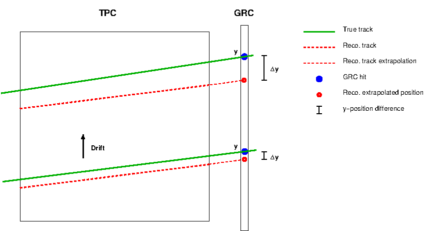
Figure 1: (Color online) Illustration of the Geometry Reference Chamber (GRC) concept. The particle tracks in the TPC chamber are reconstructed with an initial estimate for the drift velocity and are paired to the hits of a segmented detector, the GRC. In case the drift velocity estimate differs from the true in-situ drift velocity inside the TPC, the mismatch along the drift coordinate gets gradually worse at increasing drift depths. The slope of the drift coordinate mismatch against the drift coordinate as measured by the GRC provides the correction between the true in-situ drift velocity versus the initial estimate.

In order to implement the GRC concept, several design requirements were considered. To reduce the development time and cost of the readout electronics, a solution using the existing TPC readout Front-End Electronics (FEE) was chosen. In order to reduce the number of readout channels, we decided to implement a simple Multi-Wire Proportional Chamber (MWPC) with cartesian readout. This required two issues to be addressed. Firstly, the signal formation in the GRC had to be slowed down sufficiently such that the signal persists until the TPC electronics begins to sample the charges. This is not entirely trivial to achieve, since TPC readout electronics typically have a microsecond-level trigger latency with respect to the particle passage time, during which the signal may already disappear from the GRC. In order to mitigate this issue, a drift volume with adjustable drift field was introduced in the GRC design, transverse to the particle passage direction, and with that the GRC signal duration could be controlled. Secondly, the cartesian readout scheme tends to be problematic whenever the particle occupancy is large. In order to overcome this limitation, the GRC acceptance was designed to be variable: for low-multiplicity type of collisions, the entire GRC acceptance can be used, whereas for high-multiplicity collisions, individual anode wires (sense wires) of the GRCs can be disabled, down to a single amplifying wire. This helps reduce the number of combinatorial ghost hits.

The structure of the paper is as follows. In Section 2 an overview of the NA61/SHINE experimental facility is given. In Section 3 the GRC design requirements, parameters, and implementation are discussed. In Section 4 the operational performance is shown. In Section 5 a conclusion is provided. The paper is closed by Appendix A and Appendix B discussing the details of systematic errors and the calibration of further geometry-related TPC calibration constants, where the GRC chamber plays a role.

2 The NA61/SHINE experimental facility

The NA61/SHINE [2] is a fixed-target hadron spectrometer experiment at the CERN SPS accelerator. Large parts of its tracking devices were inherited from a previous experiment called NA49 [3]. Its physics program covers the study of strongly-interacting matter via heavy-ion collisions and measurements of identified particle production spectra in hadron-nucleus collisions as reference data for flux prediction in long baseline neutrino experiments (T2K, DUNE) and large area cosmic ray observatories (Pierre Auger Observatory).

An overview of the NA61/SHINE experiment is shown in Fig.2. Two large superconducting bending magnets (Vertex-I and II) are responsible for particle deflection for charge and momentum determination. Their total maximum bending power is ${\sim}9\,\mathrm{Tm}$ (up to $1.5\,\mathrm{Tesla}$ magnetic field in Vertex-I and $1.1\,\mathrm{Tesla}$ in Vertex-II). A target holder with target-in / target-out moving capability sits just upstream of the first Vertex TPC. Thin targets can be placed inside a silicon Vertex Detector (VD) for precise vertex determination. NA61/SHINE also has the ability to measure interactions in extended replica targets for long baseline neutrino experiments. The tracking devices for spectrometry are composed of eight large volume TPCs (total ${\sim}40\,\mathrm{m}^{3}$ and ${\sim}1\,\mathrm{m}$ drift length), capable of performing both tracking and $\mathrm{d}E/\mathrm{d}x$ measurements. An MRPC-based Time-of-Flight wall (L-ToF) provides further particle identification (PID) capabilities around mid-rapidity, whereas a scintillator based Time-of-Flight wall covers (F-ToF) covers the forward phase space, enabling two-dimensional (ToF+$\mathrm{d}E/\mathrm{d}x$) separation of particle species at large parts of the acceptance. A calorimeter is placed at the end of the beamline, called the Projectile Spectator Detector (PSD), which helps to characterize collision centrality in heavy-ion collisions, and consists of two compartments (MPSD and FPSD) for optimal shower containment. Upstream of the target position, a set of beam position detectors (BPDs), scintillator and Cherenkov detectors serve as beam and beam PID trigger (not shown in the figure). On the beamline between VTPC-1 and the GapTPC, a small plastic scintillator with a $1\,\mathrm{cm}$ diameter serves as an interaction trigger in most collision types (S4). In rare run settings, a very similar scintillator (S5) just upstream of MPSD is used instead. For heavy-ion runs the scintillator (S3) just downstream of VD is used for interaction definition through detecting loss of charge (i.e., by sensing a decreased $Z^{2}$ with respect to the beam nuclei). The VD, the new silicon BPDs, the MRPC-based L-ToF, the MPSD and FPSD were introduced during the Long Shutdown 2 (LS2) upgrade period between 2019-2021. Also during LS2, the data acquisition (DAQ) was upgraded, allowing for an event recording rate up to $1.8\,k\mathrm{Hz}$ for the detector complex.

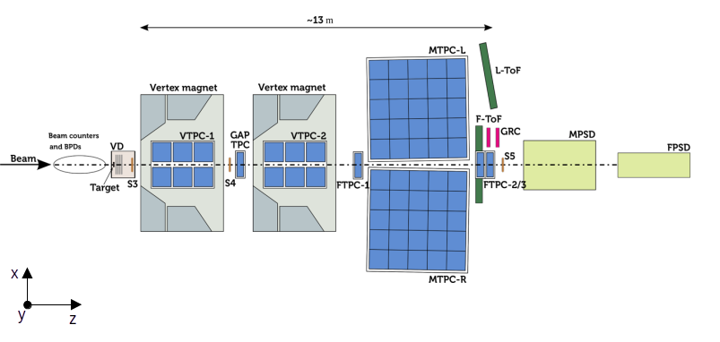
Figure 2: (Color online) The NA61/SHINE detector configuration, after the Long Shutdown 2 (LS2) upgrade, i.e. since 2022. The drawing shows the top view of the bending plane. That is, the approximately homogeneous magnetic field inside the Vertex-I and Vertex-II magnets is perpendicular to the figure. The electric drift field of the TPCs is also perpendicular to the figure. The GRC system for in-situ drift velocity monitoring was also conceptualized and introduced during the LS2. The GRC system, as of now, consists of two adjacent identical chambers (GRC-1 and GRC-2), for redundancy reasons.

The concept of the Geometry Reference Chambers (GRCs), just downstream of MTPC-L, was also developed during the LS2 upgrade period. Its lightweight design was motivated by short development time, and relatively fast and low risk implementability. In addition, the TPC chambers were moved during the LS2 upgrade, and therefore seven calibration constants apart from the drift velocity must be re-determined. These are the trigger latency, the three-dimensional alignment shifts, and the three alignment angles for each TPC. These are too many unknowns to determine without an absolute reference. The GRC enables unambiguous determination of all seven parameters and the drift velocity.

3 The GRC system

The NA61/SHINE TPCs have a drift length of ${\sim}1\,\mathrm{m}$ and are capable of resolving particle cluster positions at the ${\sim}1\,\mathrm{mm}$ at the extremum of the drift volume. Therefore, in order to reduce the systematic errors of the position measurements below the position resolution, the in-situ drift velocity has to be determined with permil accuracy. The drift velocity in a typical TPC system is affected by the working gas composition, the electric drift field applied to the TPC, the gas temperature, and the gas pressure. Most large TPC systems, such as the TPCs in NA61/SHINE experiment or the one in ALICE [5] at CERN’s LHC, or in STAR [6, 7] at BNL’s RHIC, are equilibrated with the atmospheric pressure, with a very slight constant overpressure applied in order to avoid air inflitration. Since the gas composition, drift field and the temperature is typically stabilized, the shortest time scale variations are caused by meteorological changes in the ambient air pressure. This means that the time scale of anticipated substantial drift velocity variations are not shorter than about $5$ minutes. Therefore, the design goal of the GRC system was to have an in-situ drift velocity measurement inside MTPC-L with a permil statistical error for about every $5$ minute time window during data taking. Given the worst-case minimal particle flux, this requirement gives the lower bound to the acceptance (area) of the GRC in case of low-multiplicity collision types. In order to minimize the necessary area of the GRC, a location was chosen with the maximum possible particle flux passing through MTPC-L, but avoiding the vicinity of the beam spot. This justifies the chosen placement of the GRC system, shown in Fig.2. At the selected location, the worst-case minimum particle flux was estimated using formerly recorded proton-proton collision data at $13\,\mathrm{GeV}/c$ beam momentum. With about a factor of two safety margin, this resulted in a $40\,\mathrm{cm}$ $\times$ $120\,\mathrm{cm}$ sensitive area, with the longer dimension fully covering the drift direction of MTPC-L. For redundancy reasons, two identical GRC stations (GRC-1 and GRC-2) were placed in an adjacent position (see Fig.2).

For cost efficiency reasons, the GRC implementation was chosen to be a robust MWPC with cartesian readout loosely based on the design [8, 9], which was originally optimized for cosmic muon imaging purposes. Gas amplification is achieved on the anode wires (Sense Wires), and the transverse position information is read from adjacent wires (Field Wires) parallel to these in the same plane. For the vertical position information relevant for drift velocity monitoring, the segmentation is achieved using wires with the same functionality as cathode strips, perpendicular to the Sense Wire / Field Wire direction (those are called Pickup Wires). The design choice to use such wires instead of strips is due to easier construction of the whole chamber. For low-multiplicity data taking campaigns, the entire GRC acceptance is read out as is. For high-multiplicity runs, such as heavy-ion data taking periods, the cartesian combinatorial background becomes an issue. In order to mitigate this, the design allowed for high-voltage jumpers used to turn off individual Sense Wires. This has the effect of narrowing the transverse acceptance down to a single active sense wire. This feature completely eliminates the cartesian combinatorics, preserving the drift velocity determination accuracy in high multiplicity runs. The concept is sketched in the left panel of Fig.3.

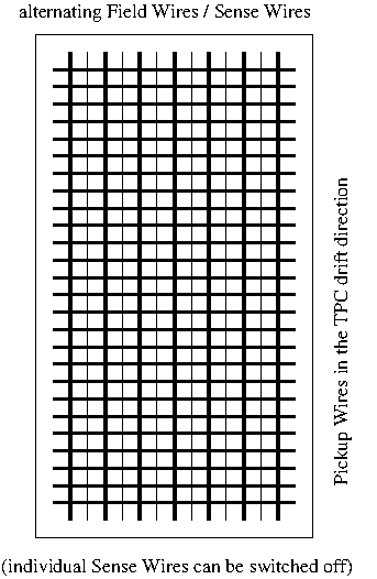
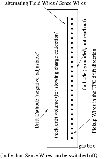
Figure 3: (Color online) Left panel: sketch of a GRC chamber as seen from the direction of the arriving particle flux (not to scale). The transverse direction is covered by the Field Wire / Sense Wire plane, where the electron multiplication takes place on the Sense Wires, and their mirror charges on the Field Wires are read out. The TPC drift direction is covered by the Pickup Wire plane, also seeing the mirror charges of the charge clouds on the Sense Wires. This provides the other cartesian coordinate for readout. Individual Sense Wires can be connected to high voltage or ground using configurable high-voltage jumpers (not drawn on the figure). Right panel: sketch of a GRC as seen from side view (not to scale). The thickness of the drift region is larger in the direction of the particle flux, and a drift cathode electrode with adjustable potential is used. This combination makes sure that the charge collection can be sufficiently slowed down such that the signal in the chamber persists until the TPC readout electronics, used for the GRC readout, begins to measure.

In order to reduce cost and development time for the readount electronics, the GRCs were designed to be read out using the existing TPC FEEs. Two TPC FEE cards are enough to read out the induced charges on the $32$ Field Wire channels $\times$ $192$ Pickup Wire channels in each GRC. A natural issue with this solution is that the TPC, being a relatively slow device, allows for a relatively large trigger latency. A typical TPC readout FEE is generally optimized for making meaningful charge sampling measurements only $1-2\,\mu\mathrm{s}$ after the beam passage. In order to make sure that the signal in the GRC persists until the TPC FEE begins to take meaningful charge samples, a $30\,\mathrm{mm}$ thick drift volume was added. This has the effect of extending charge collection over time. In order to control the signal collection timescale, an adjustable drift field electrode was added to the design. The signal stretching concept is shown schematically in the right panel of Fig.3. The GRC front-end readout system is fully integrated with the NA61/SHINE Data Acquisition System (DAQ). GRC-specific event reconstruction software is fully integrated with the NA61/SHINE offline software (ShineOffilne) [10]. The fundamental parameters of the MWPC design of the GRCs are listed in Table 1.

chassis	FR4 bars and typical PCB board material
typical working gas	$\mathrm{Ar}(80):\mathrm{CO}_{2}(20)$ at $5\,\mathrm{l/h}$ flow
typical Drift Cathode potential	$0\,\mathrm{V}$
Field Wire and Pickup Wire potential	$0\,\mathrm{V}$
typical Sense Wire potential	$1580\,\mathrm{V}$
Pickup Wire	CuZn40 (EDM Tec) $100\,\mu{}\mathrm{m}$, $70\,\mathrm{g}$ tension
Field Wire	CuZn40 (EDM Tec) $100\,\mu{}\mathrm{m}$, $70\,\mathrm{g}$ tension
Sense Wire	Au coated W (Luma Metall) $20\,\mu{}\mathrm{m}$, $15\,\mathrm{g}$ tens.
Field Wire to Sense Wire distance	$6\,\mathrm{mm}$
distance between adjacent Pickup Wires	$3\,\mathrm{mm}$ (read out pairwise)
FW/SW to Pickup Wire plane distance	$10\,\mathrm{mm}$
Pickup Wire plane to cathode backplane dist.	$2\,\mathrm{mm}$
Drift Cathode to FW/SW plane	$30\,\mathrm{mm}$
number of Sense Wires	$31$
number of Field Wires	$32$
number of Pickup Wire pairs	$192$

Table 1: Design parameters of the GRC MWPCs.

Since the GRC performs a differential measurement along the TPC drift direction, precise alignment of the GRCs with respect to the TPC is not critical. However, if the TPC-GRC alignment is known, the GRC system can be used to determine a further calibration constant: the trigger latency ($t_{0}$). In order to make use of this possibility, care was taken in the design such that the position of the optical survey target for geodesic localization of the GRCs can be accurately related to the internal wire positions. A CAD sketch of the sensor plane and a photograph of the installed GRC system is seen in Fig.4.

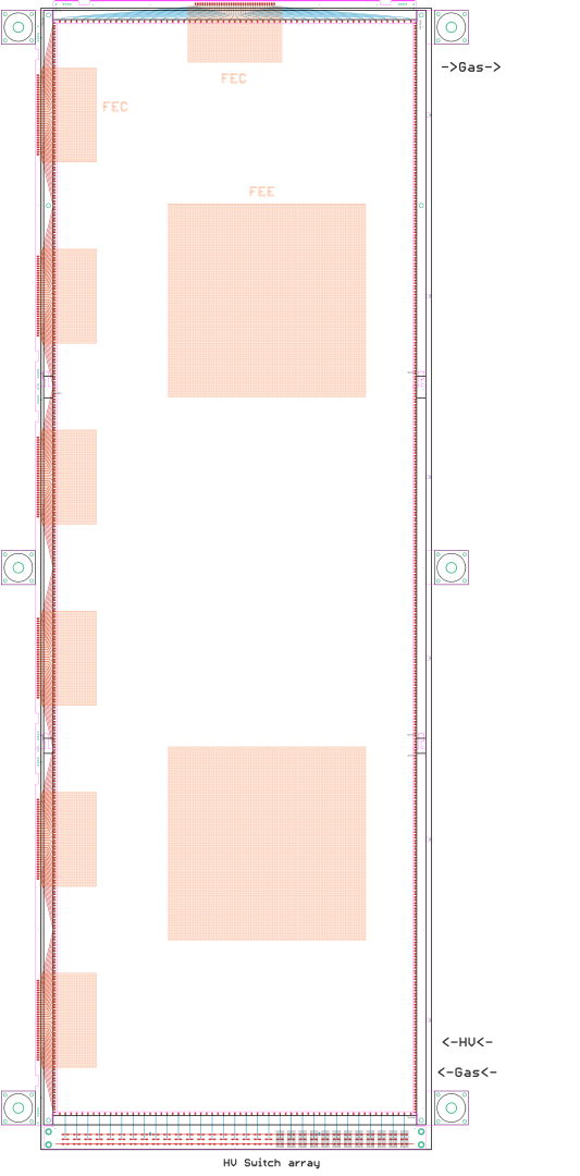
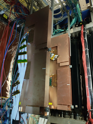
Figure 4: (Color online) Left panel: the PCB CAD snapshot of the sensor layer of a GRC chamber. The six holders for the optical geodesic survey targets are well visible. By design, these are precisely relatable to the internal wire geometry. Right panel: the photograph of the installed GRC system as seen looking upstream. The black wall is the F-TOF, covering the downstream plane of MTPC-L. The upstream chamber is GRC-1, whereas the downstream chamber is GRC-2.

4 Drift velocity calibration using the GRC

Drift velocity calibration via the GRC is based on track matching between MTPC-L and the GRC as sketched in Fig.1, and subsequently using GRC as a differential length scale. If the drift velocity estimate differs from the true drift velocity, the TPC drift coordinate versus GRC coordinate mismatch has a slope as a function of the GRC coordinate. This slope can be used for calibration. Tracks are typically collected over the course of 5 minutes of data taking, providing a drift velocity estimate spanning those 5 minutes.

The calibration equations can be derived as follows. The NA61/SHINE coordinate convention, as seen in Fig.2, is that the global cartesian $x$ coordinate is from MTPC-R to MTPC-L, the global $y$ coordinate is from down to up, and the global $z$ coordinate is along the nominal beamline from upstream toward downstream. Similarly oriented $x$, $y$, $z$ cartesian local coordinates are also used within each chamber. The TPC drift coordinate is the $y$ local coordinate, by convention, and the drift is from negative to positive direction, whereas the local $x$ coordinate is along the readout pads of a padrow (along the Sense Wires of the TPC), and the local $z$ coordinate is stepping in between pad rows. For a TPC chamber, one has that

$$y_{\mathrm{nom}} = y_{\mathrm{anode},\mathrm{nom}}-(t_{0,\mathrm{nom}}+t_{\mathrm{drift,raw}})\cdot v_{\mathrm{drift,nom}},$$ (4.1)

$$y_{\mathrm{true}} = y_{\mathrm{anode},\mathrm{true}}-(t_{0,\mathrm{true}}+t_{\mathrm{drift,raw}})\cdot v_{\mathrm{drift,true}}.$$ (4.2)

Here $y_{\mathrm{nom}}$ is the reconstructed drift coordinate assuming a nominal estimate during reconstruction for the position of the TPC amplification plane at $y_{\mathrm{anode},\mathrm{nom}}$. The symbol $t_{0,\mathrm{nom}}$ stands for a nominal estimate for the trigger latency during reconstruction. $t_{\mathrm{drift,raw}}$ is the measured particle track cluster position in terms of drift time as measured by the TPC readout. $v_{\mathrm{drift,nom}}$ is the nominal estimate for the electron drift velocity in the TPC during reconstruction. The quantities labeled by $\,{()}_{\mathrm{true}}\,$ are the true but unknown values of these calibration factors. The negative sign in Eq.(4.2) is due to the coordinate convention in NA61/SHINE. The coordinate $y_{\mathrm{nom}}$ measured by the TPC along the drift direction corresponds to a GRC measurement $y_{\mathrm{true}}$, for each track matched to a GRC hit, as seen in Fig.1. The matching is done via a typically ${\sim}3\,\mathrm{cm}$ wide tolerance window. By eliminating the running variable $t_{\mathrm{drift,raw}}$ in Eq.(4.2), one infers

$$\Delta{y} = \underbrace{\left(v_{\mathrm{drift,nom}}/v_{\mathrm{drift,true}}-1\right)}_{\mathrm{slope}}\cdot y_{\mathrm{true}}$$ (4.3)

. $$\qquad\;+\;\underbrace{\left(y_{\mathrm{anode,nom}}-v_{\mathrm{drift,nom}}/v_{\mathrm{drift,true}}\cdot y_{\mathrm{anode,true}}+v_{\mathrm{drift,nom}}\cdot(t_{0,\mathrm{true}}-t_{0,\mathrm{nom}})\right)}_{\mathrm{offset}}$$ (4.4)

for the ensemble of TPC-GRC tracks. Here $\Delta{y}:=y_{\mathrm{nom}}-y_{\mathrm{true}}$ stands for the drift coordinate TPC-GRC mismatch and $y_{\mathrm{true}}$ stands for the GRC measurement. Occasionally, the label $()_{\mathrm{true}}$ will be suppressed where not confusing. The slope of the $\Delta{y}$ versus $y$ scatter plot determines the correction factor between the true drift velocity $v_{\mathrm{drift,true}}$ and the estimate $v_{\mathrm{drift,nom}}$ assumed during the reconstruction, thus $v_{\mathrm{drift,true}}$ can be determined from the TPC-GRC mismatch data. This is shown in Fig.5 top panel for a typical low-multiplicity data set (proton-carbon collisions at $120\,\mathrm{GeV}/c$ beam momentum, recorded in 2023). In Fig.5 bottom left panel the same is shown, but for a typical high-multiplicity data set (minimum-bias Pb+Pb collisions at $150\,A\mathrm{GeV}/c$ beam momentum, recorded in 2022). Fig.5 bottom right panel shows the same high-multiplicity data set with only a single Sense Wire switched on, thus eliminating the cartesian combinatorial ghost hits using the design feature explained in Section 3.

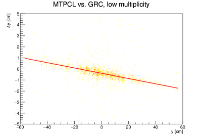
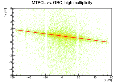
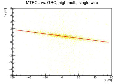
Figure 5: (Color online) Top panel: an example for the $\Delta{y}$ versus $y$ drift velocity calibration method on a real data sample in a $5$-minute time window. The corresponding data set is a low multiplicity run (proton-carbon collisions at $120\,\mathrm{GeV}/c$ beam momentum, recorded in 2023). Here, the full GRC acceptance was used. Bottom left panel: the equivalent plot for a high multiplicity run, with the full GRC acceptance (minimum-bias Pb+Pb collisions at $150\,A\mathrm{GeV}/c$ beam momentum, recorded in 2022). Bottom right panel: the same high multiplicity data set with only a single Sense Wire used, thus eliminating the cartesian combinatorial ghost hits in GRC. Note the substantially-reduced background. The color scale is merely to emphasize hit density.

In order to further suppress the combinatorial background accompanying the correlation signalsignal, the ROOT implementation of the Least Trimmed Squares (LTS) fitting was used. After calibrating MTPC-L, the upstream chambers are subsequently calibrated step-by-step using downstream chambers as geometric references.

The statistical uncertainty of the method can be estimated from above by treating the pickup wire electrodes as $6\,\mathrm{mm}$ wide strips. Thus, the single-track position resolution of the GRC is not worse than $6\,\mathrm{mm}/\sqrt{12}$, corresponding to the resolution of a $6\,\mathrm{mm}$ wide uniform distribution. For a track sample of a ${\sim}5\,\mathrm{minute}$ time window, typically there are hundreds of MTPC-L tracks hitting the GRC. It is thus possible to reach the desired statistical uncertainty of $1\,\mathrm{mm}$, corresponding to $1$ per mil of the ${\sim}1\,\mathrm{m}$ TPC drift length. The systematic accuracy of the method was quantified using a closure test. By re-reconstructing the data using the calibrated drift velocities, the calculated correction on top of the previously-corrected drift velocities was found to be better than 1-2 permil. This can be attributed to the systematic uncertainty of the method. The systematics were also double-checked by comparing the obtained drift velocities to the exhaust analysis method, which agreed within 1-2 permil, up to a normalization constant. Note that the exhaust analysis method is expected to have worse systematics in comparison to the more-direct $\Delta{y}$ versus $y$ method discussed in this paper. These validation plots are seen in Fig.6.

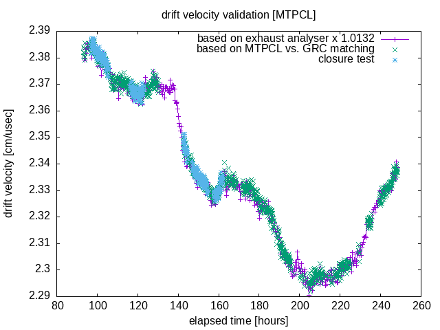
Figure 6: (Color online) Final validation of the GRC-based $\Delta{y}$ versus $y$ drift velocity calibration method. It is seen that the closure test is satisfied to the desired accuracy (1-2 permil). Moreover, good consistency is seen with the exhaust analyzer method. (Note that the exhaust analyzer method is expected to have some absolute systematic error, hence the necessity for its normalization scale adjustment.)

5 Concluding remarks

In this paper a novel cost-efficient method was described for in-situ drift velocity monitoring in large volume TPCs. The method was deployed and is currently in use at the NA61/SHINE experiment at CERN. The key idea is to place a low-cost segmented detector, called to be the Geometry Reference Chamber (GRC), downstream of the TPC to be monitored. This monitoring solution was added retrospectively to the existing TPC system without a surgical operation to the chambers. A GRC was cost-effectively realized by using a MWPC designed to be compatible with existing TPC readout electronics. In such a way the development time and cost of the readout electronics could be spared. In order to match such an MWPC to the TPC readout electronics, it was necessary to slow down the signal formation in the GRC, since TPC readout electronics typically posses a considerable trigger latency. This signal slowing was achieved by using an adjustable drift field transverse to the particle passage direction. The number of required readout channels was minimized using cartesian readout. Since the NA61/SHINE experiment is used to study both low- and high-multiplicity collisions, the acceptance of the GRC was designed to be sufficiently large while addressing the issue of combinatorial ghost hits. The latter was handled by making the acceptance adjustable: when studying high-multiplicity collisions, individual Sense Wires can be switched off down to a single wire, eliminating the cartesian ghosts, whereas for low-multiplicity runs the full acceptance is used with all of the Sense Wires operational.

The GRC system has been demonstrated of being capable of monitoring the drift velocity down to a one permil absolute precision in about $5$ minute time windows. That is, the pertinent method is applicable to large drift length TPC systems, with minimal design time, and relatively low manpower and cost.

Motivated by the GRC-based drift velocity monitoring method, a calibration procedure for the other geometric calibration parameters of the NA61/SHINE TPC chambers was also developed. Using that concept, all 8 parameters (time-dependent drift velocity, trigger latency, alignment shifts, and alignment angles) of the TPC system were successfully calibrated.

Appendix

Appendix A Trigger latency and drift-direction alignment of TPCs

After the drift velocity has been calibrated with the $\Delta{y}$ versus $y$ method, one has $v_{\mathrm{drift,nom}}\approx v_{\mathrm{drift,true}}$, and therefore the TPC-GRC drift coordinate mismatch becomes $y$-independent, expressable as

$$\Delta{y} = \underbrace{(t_{0,\mathrm{true}}-t_{0,\mathrm{nom}})}_{\mathrm{slope}}\cdot v_{\mathrm{drift}}\;+\;\underbrace{(y_{\mathrm{anode,nom}}-y_{\mathrm{anode,true}})}_{\mathrm{offset}}$$ (A.1)

as seen from Eq.(4.4). Taking several data samples with in-situ drift velocity differing by $1-2\%$, the slope of the $\Delta{y}$ versus $v_{\mathrm{drift}}$ scatter plot provides the additive correction between the true trigger latency ($t_{0,\mathrm{true}}$) against the trigger latency estimate applied during the reconstruction ($t_{0,\mathrm{nom}}$). Thus, $t_{0,\mathrm{true}}$ can be determined from the TPC-GRC mismatch data. After the $t_{0}$ is calibrated, the TPC-GRC mismatch will be not only $y$-independent, but also $v_{\mathrm{drift}}$-independent, and one is left with $\Delta{y}=y_{\mathrm{anode,nom}}-y_{\mathrm{anode,true}}$. Thus, the drift direction displacement ($y$-alignment correction) $y_{0}:=y_{\mathrm{anode,nom}}-y_{\mathrm{anode,true}}$ of the TPC versus the GRC can be determined from the TPC-GRC mismatch data. An example for the $\Delta{y}$ versus $v_{\mathrm{drift}}$ calibration method is shown in Fig.7. Having the $t_{0}$ and $y_{0}$ obtained, the upstream TPC chambers can also be calibrated, using the already calibrated TPCs as geometry reference, in place of the GRC.

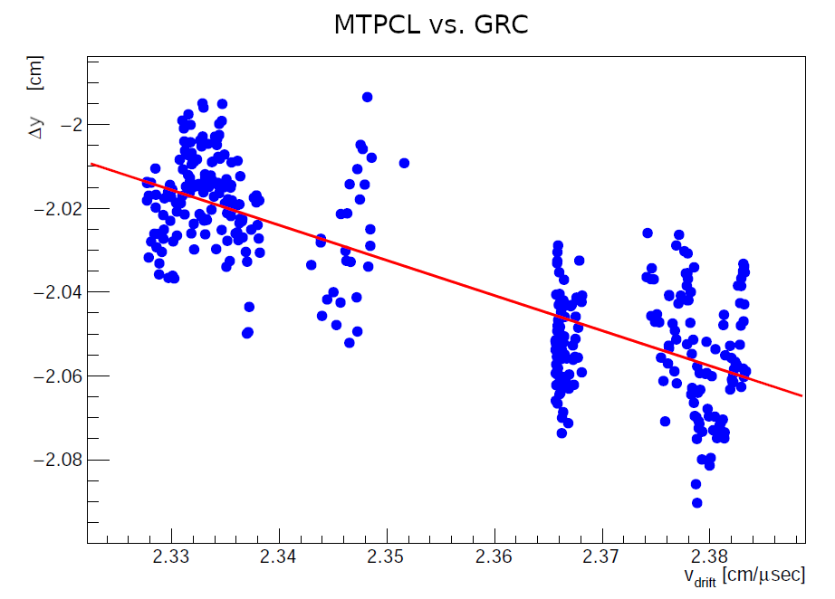
Figure 7: (Color online) An example for the $\Delta{y}$ versus $v_{\mathrm{drift}}$ analysis for trigger latency ($t_{0}$) and drift direction shift ($y_{0}$) calibration, after the drift velocity ($v_{\mathrm{drift}}$) has been obtained. The slope of the pertinent scatter data gives the $t_{0}$ correction, whereas the offset gives the $y_{0}$ correction. For the method to be workable, data samples with different drift velocities (up to $1-2\%$) are used. The pertinent data set is a high multiplicity collision type (minimum-bias Pb+Pb collisions at $150\,A\mathrm{GeV}/c$ beam momentum, recorded in 2022).

In the calibration database, for each TPC, the $t_{0}$ information is stored as follows. The $t_{0}$ for one of the TPCs (MTPC-L) is stored as a global reference (called to be the global $t_{0}$). For the other TPCs, only their relative $t_{0}$ difference with respect to this reference TPC is stored (called to be the chamber $t_{0}$). The rationale in such separation of the global and chamber $t_{0}$ contributions is the following. The chamber $t_{0}$ values are supposed to be detector constants, as they can only depend on cable lengths and electronic delays with respect to the trigger system. The global $t_{0}$, however, can also depend on the physics settings, such as beam time-of-flight, custom settings of delays inside the trigger logic etc. Thus, it is safer to recalibrate the global $t_{0}$ (MTPC-L versus GRC) for each data taking campaign, whereas it is enough to determine the relative chamber $t_{0}$ constants (other TPCs versus MTPC-L) only once, as they are detector constants. The recalculated relative chamber $t_{0}$ values are used, though, for consistency checks and quality monitoring.

Appendix B Systematic errors and alignment calibration of the TPCs

As summarized in Section 4, the final systematics of the in-situ drift velocity calibration via the $\Delta{y}$ versus $y$ method was verified to be not worse than 1-2 permil (or $1\,\mathrm{mm}$ overall, along the ${\sim}1\,\mathrm{m}$ drift length). This performance, however, was only achievable after some detailed studies. The main systematics error comes from a possible misalignment of the adjacent chambers, or misalignment of MTPC-L versus the GRC. Assume that we have a pair of TPC chambers, to be calibrated against each-other from the point of view of drift velocity. Assume moreover that the downstream one is either the GRC, or is an already drift velocity calibrated TPC. Using automatic formula manipulation programs (e.g. Maple) evaluating affine transformations is not difficult, and it is rather straightforward to show that if the upstream chamber has an imperfectly known alignment, that contributes to the multiplicative drift velocity correction $v_{\mathrm{drift,corr}}:=v_{\mathrm{drift,true}}/v_{\mathrm{drift,nom}}$ obtained by the $\Delta{y}$ versus $y$ in-situ drift velocity calibration method, described in Section 4. The track-by-track systematics is seen to be

$$\mathrm{syst}(v_{\mathrm{drift,corr}})=\Big{(}y\cdot\theta_{x}+x\cdot\theta_{y}+(y-y_{\mathrm{mainvertex}})\cdot\theta_{x}+z_{0}\Big{)}\cdot\frac{1}{z-z_{\mathrm{mainvertex}}}$$ (B.1)

to the first order. Here, $x,y,z$ is the particle hit position at the $z=const$ reference plane (e.g. the GRC plane) of the $\Delta{y}$ versus $y$ study, moreover $x_{0},y_{0},z_{0}$ denote the (unkown) correction to the position alignment of the upstream chamber, and $\theta_{x},\theta_{y},\theta_{z}$ denote the (unknown) correction to the angular alignment of the upstream chamber, whereas the $x,y,z$ coordinates indexed by $()_{\mathrm{mainvertex}}$ denote the coordinates of the collision point. It is seen that the drift velocity systematics decreases with distance from the main-vertex, and therefore justifies our placement of the GRC downstream of all the TPCs, as seen in Fig.2. Even if the angular or position alignment of the MTPC-L with respect to the GRC were imperfectly known to $|y\cdot\theta_{x}|\lesssim 1\,\mathrm{cm}$ or $|x\cdot\theta_{y}|\lesssim 1\,\mathrm{cm}$ or $|(y-y_{\mathrm{mainvertex}})\cdot\theta_{x}|\lesssim 1\,\mathrm{cm}$ or $|z_{0}|\lesssim 1\,\mathrm{cm}$, since $|z_{{}_{\mathrm{GRC}}}-z_{\mathrm{mainvertex}}|\approx 16\,\mathrm{m}$, this would not disturb the MTPC-L versus GRC drift velocity calibration, beyond half a permil. That is, the alignment imperfection does not give sizable systematics to the MTPC-L versus GRC in-situ drift velocity calibration. When propagating the drift velocity calibration toward the upstream chambers (VTPC-1, VTPC-2), however, the systematics Eq.(B.1) by imperfectly known alignment can give a sizable contribution. Therefore, in this appendix we briefly describe, how the alignment is calibrated.

A TPC chamber has in total 8 unknown calibration coefficients related to its geometry: the $x_{0},y_{0},z_{0}$ position misalignment correction (transverse, drift direction, longitudinal), the $\theta_{x},\theta_{y},\theta_{z}$ angular misalignment correction, the drift velocity correction $(v_{\mathrm{drift,corr}}-1)$, and the correction to the trigger latency $t_{0,\mathrm{corr}}:=t_{0,\mathrm{true}}-t_{0,\mathrm{nom}}$. These unkown imperfection parameters, to be determined by the calibration procedure, are small, and therefore, correction to the first order Taylor expansion terms with respect to these is enough. We use special magnetic field-off calibration runs in order to have only straight trajectories for charged particle tracks throughout the chamber system. In other words, the chamber system is tomographed by an ensemble of straight global tracks associated to the main-vertex, and their mismatch pattern is studied when dissected and refitted by straight lines in the local detectors, as illustrated in Fig.8.

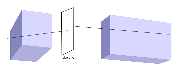
Figure 8: (Color online) Sketch of the alignment calibration strategy for adjacent TPCs: special magnetic field-off alignment calibration runs are recorded, i.e. the chamber system is tomographed by straight global main-vertex tracks. If the relative alignment parameters for the chambers assumed during the reconstruction are imperfect, the track parameters will have a mismatch, when compared on a joint reference plane, for the adjacent chambers.

Quantitatively, the magnetic field-off data based alignment calibration goes as follows. For MTPC-L, the $(v_{\mathrm{drift,corr}}-1)$ parameter is determined as in Section 4, and the parameters $t_{0,\mathrm{corr}}$,$y_{0}$ are determined as in Appendix A, whereas $\theta_{x}=\theta_{y}=\theta_{z}=0$ and $x_{0}=z_{0}=0$ by convention, i.e. MTPC-L is taken as alignment reference. The other chambers are calibrated against each-other pairwise, for all the 8 parameters, assuming that e.g. the downstream one is already calibrated. An imperfection in the assumption about the 8 parameters of the upstream chamber causes a mismatch between locally refitted track pieces in the adjacent chambers, when compared on a $z=const$ reference plane, see again Fig.8. If the straight track segments are parameterized by the four parameters $N_{x},N_{y},M_{x},M_{y}$ as $x=M_{x}+(z-z_{\mathrm{ref}})\cdot N_{x}$ and $y=M_{y}+(z-z_{\mathrm{ref}})\cdot N_{y}$, then the locally refitted and compared local tracks will give a track parameter mismatch vector field $\Delta{N}_{x},\Delta{N}_{y},\Delta{M}_{x},\Delta{M}_{y}$ as a function of the track parameters $N_{x},N_{y},M_{x},M_{y}$ in the downstream chamber (which is already calibrated or reference). Evaluating affine transformations, one arrives at the formula

$$\Delta{N}_{x} = (1+N_{x}^{2})\cdot\theta_{y}+N_{y}\cdot(N_{x}\cdot\theta_{x}+\theta_{z}),$$ (B.2)

$$\Delta{N}_{y} = N_{y}^{2}\cdot(\theta_{x}+\theta_{y})+N_{y}\cdot(v_{\mathrm{drift,corr}}-1)-N_{x}\cdot\theta_{z}+\theta_{x},$$ (B.3)

$$\Delta{M}_{x} = N_{x}\cdot(M_{y}\cdot\theta_{x}+M_{x}\cdot\theta_{y}+z_{0})+z\cdot\theta_{y}+M_{y}\cdot\theta_{z}-x_{0},$$ (B.4)

$$\Delta{M}_{y} = N_{y}\cdot(M_{x}\cdot\theta_{y}+M_{y}\cdot\theta_{x}+z_{0})+z\cdot\theta_{x}-M_{x}\cdot\theta_{z}-y_{0}$$ (B.6)

$$\qquad+(M_{y}-y_{\mathrm{anode,nom}})\cdot(v_{\mathrm{drift,corr}}-1)-t_{0,\mathrm{corr}}\cdot v_{\mathrm{drift,nom}}$$

for the mismatch field, to the first order, given the 8 imperfection parameters $\theta_{x},\theta_{y},\theta_{z}$, $x_{0},z_{0}$, $(v_{\mathrm{drift,corr}}-1)$, $t_{0,\mathrm{corr}}$, $y_{0}$. For practical reasons, the track sample satisfying $|N_{y}|\approx 0$, i.e. close to horizontal tracks are used, since for these the first two lines of Eq.(B.6) simplifies as

$$\mathrm{for\;}|N_{y}|\approx 0,\mathrm{one\;has}:$$ (B.7)

$$\Delta{N}_{x} = (1+N_{x}^{2})\cdot\theta_{y},$$ (B.8)

$$\Delta{N}_{y} = -N_{x}\cdot\theta_{z}+\theta_{x}.$$ (B.9)

That is, for magnetic field-off data, for $|N_{y}|\approx 0$ main-vertex tracks, from the $\Delta{N}_{x}$ versus $N_{x}$ plot the parameter $\theta_{y}$ can be read off, whereas from the $\Delta{N}_{y}$ versus $N_{x}$ plot the parameters $\theta_{x}$ and $\theta_{z}$ can be read off, see Fig.9 top panels. After re-reconstructing with the obtained $\theta_{x},\theta_{y},\theta_{z}$ angular alignment corrections, the third line of Eq.(B.6) yields

$$\Delta{M}_{x} = N_{x}\cdot z_{0}-x_{0}.$$ (B.10)

That is, for magnetic field-off data, from the $\Delta{M}_{x}$ versus $N_{x}$ plot the parameters $x_{0}$ and $z_{0}$ can be read off, see Fig.9 bottom panel.

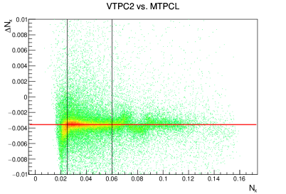
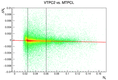
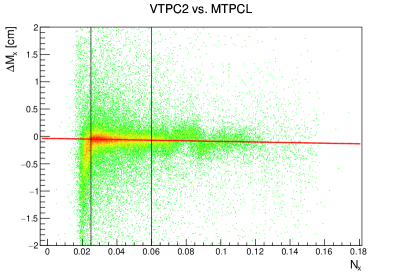
Figure 9: (Color online) Top panels: an example for the $\theta_{x},\theta_{y},\theta_{z}$ angular alignment calibration using $\Delta{N}_{x}$ versus $N_{x}$ and $\Delta{N}_{y}$ versus $N_{x}$ plots for $|N_{y}|\approx 0$ tracks in magnetic field-off data (the pertinent sample is minimum-bias Pb+Pb at $150\,A\mathrm{GeV}/c$ beam momentum, recorded in 2022). Bottom panel: an example for the $x_{0},z_{0}$ position alignment calibration using $\Delta{M}_{x}$ versus $N_{x}$ plot for tracks in magnetic field-off data (using the same sample as for the top panels). The black vertical lines indicate fiducial cuts, in order to avoid regions close to the TPC field cages, where the drift electric field can be imperfect (inhomogeneus). The color scale is merely for emphasizing hit density.

After re-reconstruction with the obtained $\theta_{x},\theta_{y},\theta_{z}$ angular alignment corrections and the $x_{0},z_{0}$ alignment shift corrections, the fourth line of Eq.(B.6) yields

$$\Delta{M}_{y} = M_{y}\cdot(v_{\mathrm{drift,corr}}-1)-y_{\mathrm{anode,nom}}\cdot(v_{\mathrm{drift,corr}}-1)-t_{0,\mathrm{corr}}\cdot v_{\mathrm{drift,nom}}-y_{0}$$ (B.11)

which is nothing but the already known Eq.(4.4), to the first order in $(v_{\mathrm{drift,corr}}-1)$, re-expressed in the notations of this appendix. That is, the drift velocity correction $(v_{\mathrm{drift,corr}}-1)$ can be determined via the usual $\Delta{y}$ versus $y$ method, as already described in Section 4. Finally, after re-reconstruction, one arrives at

$$\Delta{M}_{y} = -t_{0,\mathrm{corr}}\cdot v_{\mathrm{drift,nom}}-y_{0},$$ (B.12)

which is nothing but the already known Eq.(A.1), re-expressed in the notations of this appendix. Therefore, the remaining corrections $t_{0,\mathrm{corr}}$ and $y_{0}$ can be determined via the usual $\Delta{y}$ versus $v_{\mathrm{drift}}$ method, as already described in Appendix A. Thus, the triangular system of calibration equations for the 8 TPC geometry unkowns is saturated, and the entire TPC system can be calibrated.

After the full alignment correction, drift velocity corection, $t_{0}$ correction, $y_{0}$ correction, the overall systematics of the geometry related calibration parameters of the large TPCs, as estimated via closure tests, are listed in Table 2. The statistical errors are negligible.

	$\theta_{x},\theta_{y},\theta_{z}$ [∘]	$x_{0},z_{0}$ [$\mathrm{mm}$]	$v_{\mathrm{drift}}$ [$\%$]	$t_{0}$ [$\mathrm{ns}$]	$y_{0}$ [$\mathrm{mm}$]
	syst.	syst.	syst.	syst.	syst.
MTPC-L	$0$ (reference)	$0$ (reference)	$0.2$	$11$	$0.15$
VTPC-2	$0.038$	$0.30$	$0.2$	$33$	$0.25$
MTPC-R	$0.014$	$0.20$	$0.2$	$33$	$0.63$
VTPC-1	$0.026$	$0.25$	$0.2$	$32$	$0.07$

Table 2: The table of overall systematics of the TPC geometry parameters, for the large chambers, as estimated via closure tests. The calibration scheme was GRC $\rightarrow$ MTPC-L, followed by MTPC-L $\rightarrow$ VTPC-2, then VTPC-2 $\rightarrow$ MTPC-R and VTPC-2 $\rightarrow$ VTPC-1.

References

- [1] M. Kuich, Kaon production in mid-rapidity in Be+Be collisions at the CERN SPS, PhD thesis, University of Warsaw (2019), sections D.4 and D.5 [EDMS:2150851].
- [2] N. Abgrall et al. (the NA61 Collaboration), NA61/SHINE facility at the CERN SPS: beams and detector system, JINST 9 (2014) P06005 [arXiv:1401.4699].
- [3] S. Afanasiev et al. (the NA49 Collaboration), The NA49 large acceptance hadron detector, Nucl. Instrum. Meth. A430 (1999) 210.
- [4] A. Cattai, H. G. Fischer, A. Morelli, Drift velocity in Ar + CH4 + water vapours, DELPHI Internal Report (1989) 63.
- [5] J. Alme et al., The ALICE TPC, a large 3-dimensional tracking device with fast readout for ultra-high multiplicity events, Nucl. Instrum. Meth. A622 (2010) 316 [arXiv:1001.1950].
- [6] J. Abele et al., The Laser System for the STAR Time Projection Chamber, Nucl. Instrum. Meth. A499 (2003) 692.
- [7] M. Anderson et al., The STAR Time Projection Chamber: a unique tool for studying high multiplicity events at RHIC, Nucl. Instrum. Meth. A499 (2003) 659.
- [8] D. Varga, G. Nyitrai, G. Hamar, L. Oláh, High efficiency gaseous tracking detector for cosmic muon radiography, Advances in High Energy Physics 2016 (2016) 1962317 [arXiv:1607.08494].
- [9] D. Varga, Sz. J. Balogh, Á. Gera, G. Hamar, G. Nyitrai, G. Surányi, Construction and readout systems for gaseous muography detectors, J. Adv. Instrum. in Science 2022 (2022) 307.
- [10] R. Sipos, A. László, A. Marcinek, T. Paul, M. Szuba, M. Unger, D. Veberic, O. Wyszynski, The offline software framework of the NA61/SHINE experiment, J. Phys. Conf. Ser. 396 (2012) 022045.