Learned frequency-domain scattered wavefield solutions using neural operators

Abstract

Solving the wave equation is essential to seismic imaging and inversion. The numerical solution of the Helmholtz equation, fundamental to this process, often encounters significant computational and memory challenges. We propose an innovative frequency-domain scattered wavefield modeling method employing neural operators adaptable to diverse seismic velocities. The source location and frequency information are embedded within the input background wavefield, enhancing the neural operator’s ability to process source configurations effectively. In addition, we utilize a single reference frequency, which enables scaling from larger-domain forward modeling to higher-frequency scenarios, thereby improving our method’s accuracy and generalization capabilities for larger-domain applications. Several tests on the OpenFWI datasets and realistic velocity models validate the accuracy and efficacy of our method as a surrogate model, demonstrating its potential to address the computational and memory limitations of numerical methods.

I Introduction

Solving wave equations is pivotal for various geophysical applications like reverse time migration and full waveform inversion. However, the computational and memory bottlenecks often hinder real-time applications like microseismic imaging for CO2 monitoring. Frequency-domain simulation [1] offers a reduced dimension solution space for multi-scale waveform inversion. Yet, it still struggles with exponentially increasing memory demands with increasing model size and the necessity for repeated simulations across various frequencies.

With the development of modern machine learning techniques comes the possibility of using neural networks to surrogate numerical modeling. Physics-informed neural networks (PINNs) have recently been employed for frequency-domain wavefield modeling, demonstrating their potential in solving complex wave equations in irregular geometry through meshless solutions [2, 3, 4]. Despite their multi-frequency and multi-source capabilities [5], PINNs’ need for retraining or transfer learning for new velocities limits their generalization. Consequently, developing neural networks for a range of parametric PDEs becomes crucial. Neural operators [6] have shown great potential in solving for parametric PDEs, which provide instant PDE solutions given various coefficients and boundary conditions. Recently, they have also been used for seismic wavefield simulation, e.g., 2D time-domain wavefield simulation [7]. However, learning seismic waveform modeling in the time domain faces several challenges: (1) Learning the mapping directly from input 2D velocities and source locations to 3D wavefield volumes (spanning 2D spatial and 1D time-lapse domains) requires huge memory cost [8]; (2) Learning the mapping between the snapshots at different times within recurrent composition though decreases the memory cost, will be subject to error propagation [9] as well as the relatively huge inference cost due to the iterative nature. Thus, learning in the frequency domain using neural operators, which avoids the above limitations, could efficiently handle parametric wave equations.

Although current neural operator implementations for the frequency domain wavefield solutions offer memory efficiency, they typically often use the end-to-end framework to learn the mapping from the velocities, source locations, and frequencies to the corresponding wavefield solutions without additional feature engineering [8, 10]. Specifically, they treat the source locations as binary masks and frequencies as an additional channel for inputting neural operators with constant values. However, without considering the physics of seismic wavefields, this approach offers suboptimal inputs for convolution-based feature extraction networks. Thus, it requires additional modifications to the network architecture, e.g., paralleled Fourier neural operator [10] or limits the target frequencies of modeling [8] to make the neural operators handle various velocities and source configurations (e.g., locations and frequency) simultaneously.

To tackle this challenge, we propose learned frequency-domain scattered wavefield solutions using the Fourier neural operator. Unlike conventional methods that add source location and frequency as input channels, our proposed method implicitly embeds such information into an analytically evaluated background wavefield for a homogeneous background velocity. So, the neural operator focuses on mapping this background wavefield with the frequency and source information embedded in the scattered wavefield (or the full wavefield) for a given velocity model also as an input. The proposed method allows the neural operators to simultaneously handle the modeling for various velocities, frequencies, and source locations. Moreover, to improve generalization for larger-domain velocities beyond the training sample scope, we propose incorporating the single reference frequency [11] to enhance the generalization ability. We demonstrate the effectiveness of the proposed method on the OpenFWI dataset [12] and more realistic models, e.g., extracted from Overthrust models.

II Methodology

II-A Operator learning for Partial differential equations

Operator learning provides a stable way to build simulations for parametric PDEs, yielding a magnitude of speed-up compared to conventional numerical simulation. Parametric PDEs, in general, can be defined as

$$\mathcal{L}_{a}[u](x) =0,\quad x\in\Omega$$ (1)

where $a\in\mathcal{A}$ denotes the parameters of the operator $\mathcal{L}$, such as coefficient functions, and $u\in\mathcal{U}$ is the physical phenomenon we aim to solve for and belonging to solution space $\mathcal{U}$. The parameters and the solution are a function of location $x$ defined within domain $\Omega$. For learning an operator, we assume that, for any $a\in\mathcal{A}$, there exists a unique solution $u=\mathcal{F}(a)\in\mathcal{U}$ satisfying Eq. (1), then $\mathcal{F}$ is the solution operator of Eq. (1). Regarding the acoustic wave equation in seismic modeling, $a$ includes the source locations, frequencies, and velocity models, and $u$ represents the corresponding simulated wavefield.

The acoustic wave equation in the frequency domain (the Helmholtz equation) is formulated as follows:

$$\left(\frac{\omega^{2}}{\mathbf{v}^{2}}+\nabla^{2}\right)\mathbf{U}(\mathbf{x})=\mathbf{s},$$ (2)

where $\omega$ is the angular frequency, $\mathbf{v}$ is the velocity, $\mathbf{U}$ is the complex frequency-domain wavefield, $\mathbf{s}$ is the source term at the location $(x_{s},z_{s})$. Given a source location, a frequency, and a velocity model, we typically define a neural network $f$ with parameters $\theta$, $f_{\theta}(\mathbf{v},x_{s},z_{s},\omega)$, to represent $\mathbf{U}$.

II-B Embedding the source configurations into the background wavefield

With $f_{\theta}(\mathbf{v},x_{s},z_{s},\omega)$ and reference pre-generated modeling results as labels, we can train the neural network $f$ to act as a surrogate modeling tool. However, this approach integrates the source location and the frequency as additional input channels, with a scalar value representing frequency and a binary mask denoting the source location [7]. While structurally convenient, such representations offer limited information for effectively utilizing learned kernels in feature extraction. Instead, here, we propose embedding such information, including the frequency and the source location, in the background wavefield $\mathbf{U}_{0}$, defined, for 2D media, as:

$$\mathbf{U}_{0}(x,z)=\frac{i}{4}\boldsymbol{H}_{0}^{(2)}\left(\omega\sqrt{\frac{\left\{\left(x-x_{s}\right)^{2}+\left(z-z_{s}\right)^{2}\right\}}{\mathbf{v}_{0}^{2}}}\right),$$ (3)

where $\boldsymbol{H}_{0}^{(2)}$ is the zero-order Hankel function of the second kind, $(x_{s},z_{s})$ is the source location, $\mathbf{v}_{0}$ is the constant background velocity, and $i$ is the imaginary unit. The beauty of using background wavefield is that there is no need to specify the location of the source or the frequency while still being able to handle various source locations and frequencies. In addition, the constant background velocity can be regarded as the zero-wavenumber component of the velocity $\mathbf{v}$. Thus, the background wavefield also provides guided background information for the neural network since it controls the shape of the full wavefield. This representation or transformation of the source location and frequencies provides rich information for convolution-based feature extraction. Then, the input to the neural networks is changed from the $(\mathbf{v},x_{s},x_{z},\omega)$ to $(\mathbf{v},\mathbf{U}_{0})$.

II-C Learning for the scattered wavefield

As shown in many previous works [13, 9], learning the residual of the physical wavefield rather than directly learning the physical field itself will improve the accuracy of the neural network-based simulation. For example, Alkhalifah et al., (2020)[14] showed that solving for the scattered wavefield instead of directly learning wave equation solutions can help us avoid the point-source singularity. Inspired by those facts and considering we have a background wavefield with embedded frequency and source location information, we design the neural operator to predict the scattered wavefield, $\delta\mathbf{U}=\mathbf{U}-\mathbf{U}_{0}$, satisfying

$$\frac{\omega^{2}}{\mathbf{v}^{2}}\delta\mathbf{U}+\nabla^{2}\delta\mathbf{U}+\omega^{2}\left(\frac{1}{\mathbf{v}^{2}}-\frac{1}{\mathbf{v}_{0}^{2}}\right)\mathbf{U}_{0}=0.$$ (4)

Following the conventional supervised learning paradigm, we randomly sample source locations, frequencies, and velocities $\{v^{i},x_{s}^{i},z_{s}^{i},\omega^{i}\}$ to compute the background wavefield $U_{0}^{i}$ by solving Equation 3, and then generate the corresponding wavefield $\delta U^{i}$ by solving Equation 4 numerically for each sample. Using these samples, we train a neural network $f_{\theta}$ with input $(v^{i},U_{0}^{i})$ to predict the scattered wavefield (or the full wavefield by adding a residual connection from the input background wavefield directly to output) using a mean squared error loss

$$L(\theta)=\frac{1}{N}\sum^{N}_{i=1}{\|f_{\theta}(v^{i},U_{0}^{i})-\delta U^{i}\|_{2}^{2}},$$ (5)

where $N$ is the number of training samples. As for the choice of the neural network, we select the commonly used benchmark network, the Fourier neural operator (FNO) [6], to test the framework. The full pipeline of the approach is shown in Figure 1.

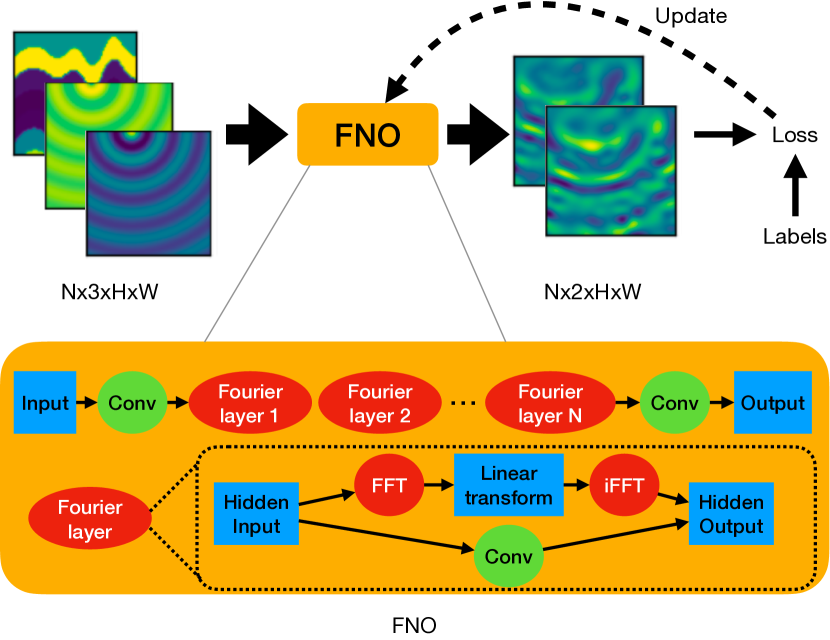
Figure 1: The pipeline of the proposed method, where the labels denote the reference results using the finite-difference method, N denotes the number of samples, and H and W are the height and width of the images. The input has three channels, including velocity and real and imaginary parts of the analytical background wavefield, while the output consists of two channels representing real and imaginary parts of the scattered wavefield. For the FNO description, we refer the reader to [6].

III Numerical Examples

We conducted tests on two velocity datasets, OpenFWI [12] and more realistic models, utilizing the Fourier Neural Operator (FNO) with four blocks (Fourier layer shown in Figure 1). Each block was configured with a truncated Fourier mode set to 48 and a Fourier layer width of 128. The activation function used here is the Gaussian Error Linear Unit (GELU) [15]. We employed an Adam optimizer to train the FNO, using a learning rate 1e-3. The training was conducted over 1000 epochs, with a batch size of 128 for the OpenFWI test and 64 for realistic models. The chosen frequency range, from 3 Hz to 21 Hz, aligns with the primary frequency band often used in seismic applications.

III-A Synthetic tests on OpenFWI dataset

Here, we first applied the proposed method to the OpenFWI dataset, focusing on the ’CurveVelA’ velocity class [12], as illustrated in Figure 3. This class of velocities includes curved layers, and the value of velocity within the layers gradually increases with depth. This test involved a comprehensive training set comprising 9,000 samples, encompassing various velocities, source locations, and frequencies, and a corresponding validating set comprising 1,000 samples. Although the Fourier neural operator can learn the mapping between infinite function space, the training data here are discretized samples with a spatial resolution of 139$\times$139. The training curve and validation error analysis are shown in Figure 2, and as we can see, the training converges well.

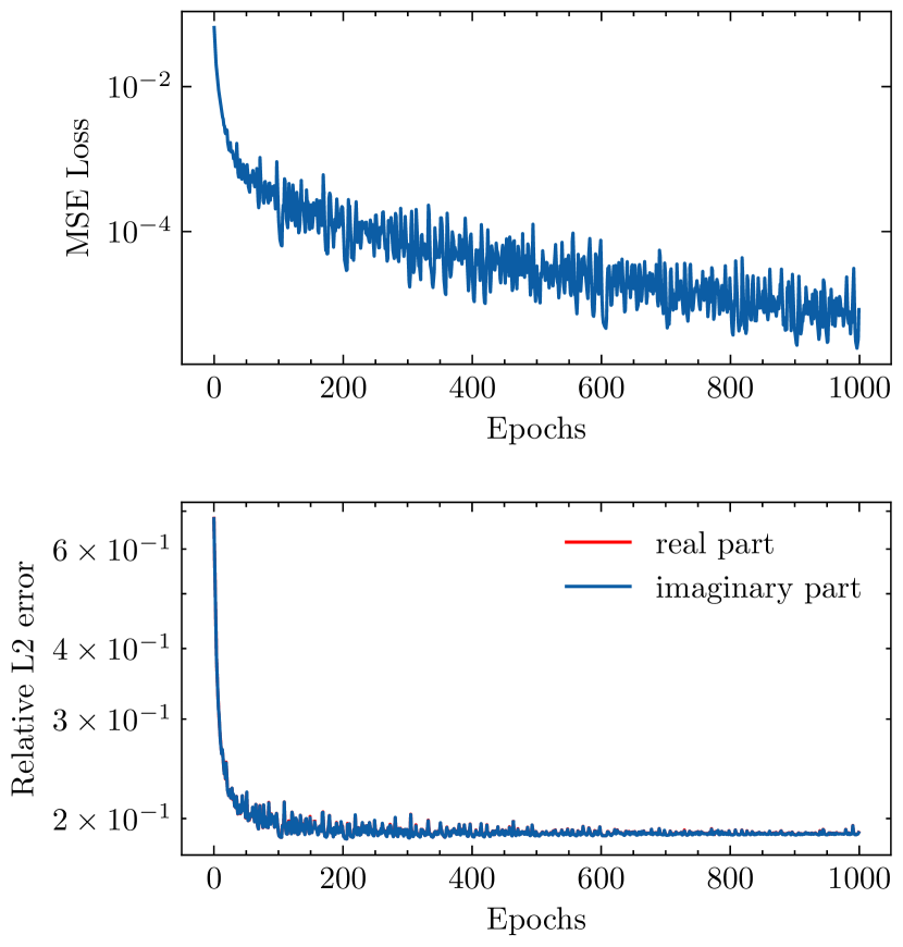
Figure 2: The training history for the ’CurveVelA’ test. Top: the training loss curve; Bottom: the validation error, which is measured by the relative L2 norm between the predictions and reference simulated results.

After the training, we evaluated the FNO for various unseen velocities, shown in Figure 4. For comparison, we use the optimal 9-point finite difference method to calculate the reference results with a spatial interval of 0.0125 km at both $x$ and $z$ directions. The predictions of FNO match well with the reference wavefields from numerical finite-difference modeling. It demonstrates that the network managed to extract the source location information and the frequency from the background wavefield and learn the relations between the various velocities and simulated complex wavefields.

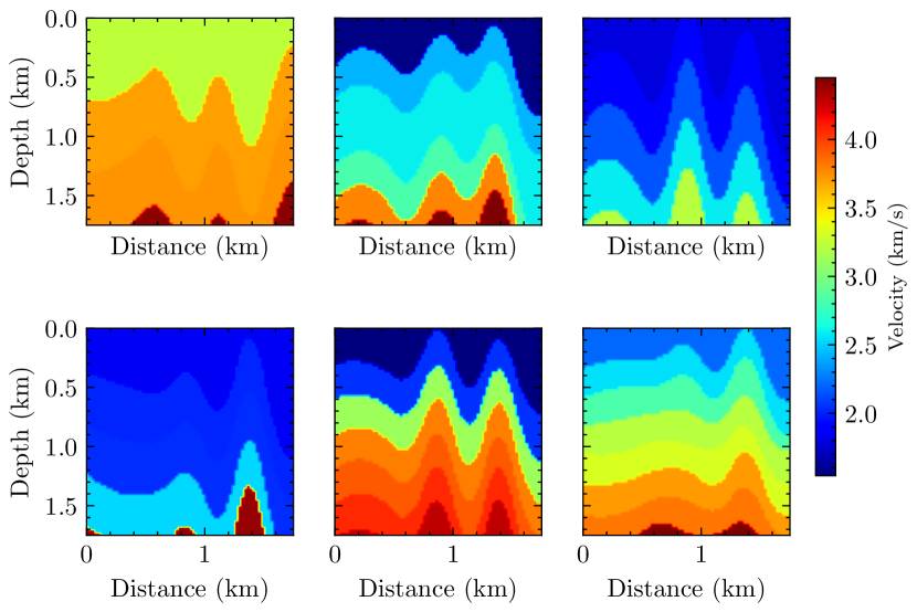
Figure 3: Samples of velocity models from the ’CurveVelA’ class.

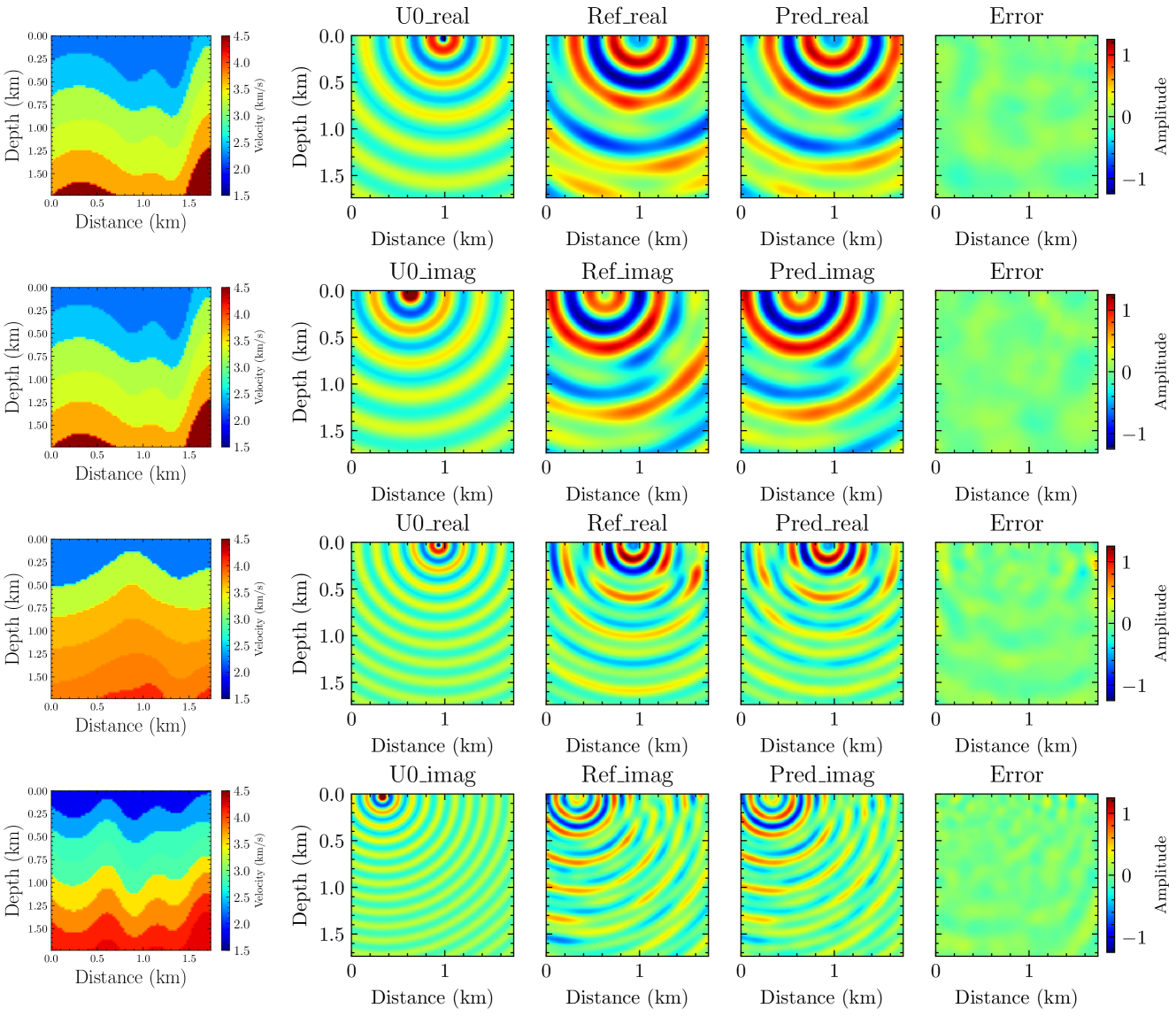
Figure 4: The results of the network predictions for velocity models (Column 1) from the test set. The plots include the background wavefield (Column 2), the reference results from numerical solutions (Column 3), the predictions (Column 4), and the difference between the predictions and the numerical solutions (Column 5). In rows 1 and 3, we show the real part of the wavefields, while in rows 2 and 4, we show the imaginary part of the wavefields. The first two rows are the results of the same velocity and same frequency of 4.25 Hz but with different source locations. The third row is the result of the prediction on another velocity but with a frequency of 7.55 Hz, while the fourth row is the result of 9.88 Hz.

III-B More realistic velocity models

To further test the effectiveness of the proposed method, we choose more realistic velocity models to test, e.g., the combinations of Overthrust, Marmousi models, and so on. Figure 5 shows samples of velocities in the training dataset. The number of training samples is 5,400, while that for validation is 600. Figure 6 shows the training loss curve and the validation error at each epoch. We also train FNO up to 1000 epochs, and it converges well. We similarly obtain the numerical reference results on unseen cases (unseen configurations of velocities, frequencies, and source locations) with a spatial interval of 0.025 km in both $x$ and $z$ directions and compare them with the predictions from the FNO. Figure 7 shows a comparison between the numerical solutions and the network predictions. Like the OpenFWI dataset tests, the FNO predicts accurate wavefields instantly.

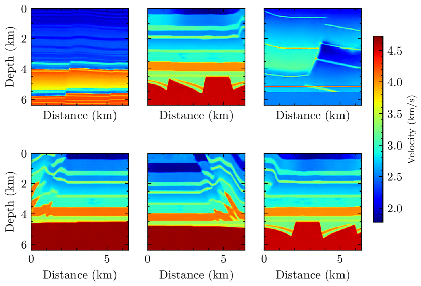
Figure 5: Samples of realistic velocity models used in the training.

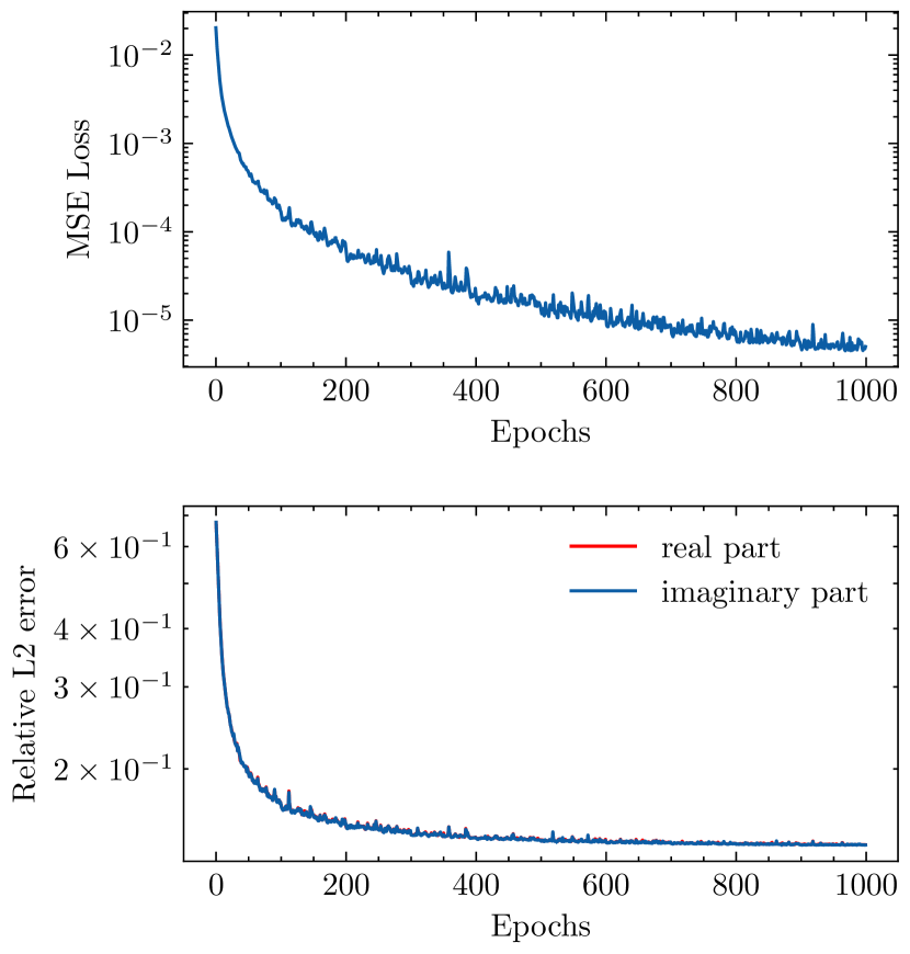
Figure 6: The training history for the realistic models test. Top: the training loss curve; Bottom: the validation error, which is measured by the relative L2 norm between the predictions and reference simulated results.

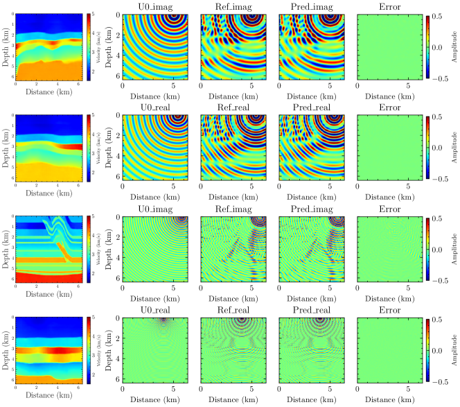
Figure 7: The results of the network predictions for four realistic velocity models in which the order of the plots are the same as in Figure 4. The frequencies for each forward modeling are, 3.93 Hz, 5.00 Hz, 12.60 Hz, and 20.66 Hz from top to bottom.

III-C Generalization test with reference frequency:

As shown in [16], FNO faces aliasing problems across different resolution scales, yielding large errors when we apply the pre-trained neural operator to predict wavefields for an unseen resolution, like when we increase the simulation domain. So, we extend our testing to evaluate the proposed method’s generalization capabilities on an unseen sample for a larger model, utilizing the concept of reference frequency. The neural network was initially trained on velocities covering an area of 6.4$\times$6.4 km² with a resolution of 256$\times$256. We then conducted a generalization test on a velocity model spanning 12.8$\times$12.8 km². with the same spatial interval. Due to the inherent resolution independence of the FNO, it seamlessly outputs the wavefield for the larger domain, which we refer to as ’direct prediction’, as depicted in Figure 8. Although the main components of the wavefield have been predicted by the FNO, their relative errors are still large. We calculate the relative L2 norm, which is the Euclidean distance from the prediction to the reference solutions divided by the Euclidean norm of the reference solutions, and the relative errors for direct predictions are 0.520 for the real part and 0.518 for the imaginary part of the wavefields. It is hard to obtain a high-accuracy prediction for a large unseen domain directly. Crucially, leveraging the reference frequency concept [11] allows us to upscale the 4.78 Hz wavefield in the large domain (12.8$\times$12.8 km²) to an equivalent 9.56 Hz wavefield in the smaller domain (6.4$\times$6.4 km²). This provides us with physical support to predict high-frequency wavefields for a large-scale velocity model rather than a direct prediction of high-resolution wavefields. As illustrated in Figure 9, this scaled wavefield demonstrates enhanced accuracy compared to direct predictions. The relative errors calculated at the resolution of 256$\times$256 between the predictions of our method without interpolation and the reference results, shown in Figure 8, are 0.052 for the real part and 0.054 for the imaginary part of the wavefield. After bilinear interpolation of the prediction using our method, the errors at a resolution of 512$\times$512 are 0.096 for the real part and 0.097 for the imaginary part of the wavefield. Though the errors slightly increase, as shown in Figure 9, the predictions using our method are still close to the reference results.

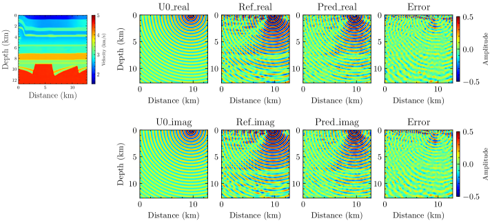
Figure 8: A generalization test on a realistic velocity model (Column 1) covering an area of 12.8$\times$12.8$km^{2}$. Column 2 shows the real and imaginary parts of the analytical background wavefield defined on 12.8$\times$12.8$km^{2}$ with an interval of 0.025 km in both $x$ and $z$ directions and with a frequency of 4.78 Hz; Column 3 represents the numerical solutions using optimal 9-point finite-difference method on a grid of 512 $\times$ 512 with a spatial interval of 0.025 $km$; Column 4 and Column 5 are the predictions using a conventional method and corresponding errors compared to the numerical solutions.

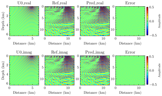
Figure 9: A generalization test on a realistic velocity model (the same velocity shown in Figure 8) using our method. The first column shows the input of our method, which are the 9.56 Hz analytical background wavefields defined on 6.4$\times$6.4$km^{2}$ with an interval of 0.025 km in both $x$ and $z$ directions. Columns 2, 3, and 4 show the numerical solutions, the predictions of our method, and the errors.

IV Discussions

The proposed method has shown good performance on the OpenFWI and realistic velocity models. It frees us at inference time from numerical simulations, in which the computational complexity is high. Taking the test on realistic models as an example, the numerical simulation, executed in parallel on an Intel(R) Xeon(R) Gold 6230R CPU @ 2.10GHz, for each velocity and frequency at a resolution of 256$\times$256 requires 6.4 seconds, and that at a resolution of 512$\times$512 requires 38.3 seconds. Using our method, the elapsed time on an NVIDIA A100 GPU (we do not fully utilize the GPU due to the relatively small input size and batch size) is 0.036 seconds for the resolution of 256$\times$256, 1.1 seconds for the resolution of 512$\times$512. Those speedups come from two main aspects: (1) we avoid repeated simulations; (2) we can easily utilize the latest hardware and software advances of accelerated computing [17] because we build the algorithm on machine learning. However, we recognize the challenges associated with the preparation of data-label pairs required for training the neural operator, particularly as the resolution of training samples increases. Additionally, the generalization capability to unseen velocities hinges on the diversity and volume of the training samples. While these challenges can be mitigated to some extent through physics-constrained learning, our focus in this paper is on introducing the neural operator with the background wavefield as input. Furthermore, the generalization prowess of our method across varied velocity models holds promising implications for applications in full waveform inversion (FWI), potentially eliminating the need for retraining and achieving real-time FWI. In our implementation, we decided to have the actual velocity as input and the scattered wavefield as output. However, the method can be equally applied by alternatively having the perturbation velocity (difference between the true and homogeneous background) as input and also the option of having the scattered or the full wavefield as output. As mentioned earlier, the full wavefield can also be obtained by employing a residual connection between the input background wavefield and the scattered wavefield.

V Conclusions

We presented a novel implementation for predicting the wavefield using the Fourier Neural Operator (FNO) by incorporating the analytically derived background wavefield as input. As a result, the source location and frequency are embedded in the background wavefield, facilitating compact and effective feature engineering. This methodology enables efficient surrogate modeling across various velocities, frequencies, and source locations. Our tests on both the OpenFWI dataset and some realistic velocity models have demonstrated the high accuracy and effectiveness of the proposed method. Additionally, incorporating a reference frequency strategy significantly enhances the accuracy of our model in generalizing to larger, unseen domain, marking a substantial advancement in the field of frequency-domain wavefield modeling.

VI Acknowledgements

We thank KAUST and the DeepWave Consortium sponsors for their support and the SWAG group for the collaborative environment. This work utilized the resources of the Supercomputing Laboratory at KAUST, and we are grateful for that.

References

- [1] K. J. Marfurt, “Accuracy of finite‐difference and finite‐element modeling of the scalar and elastic wave equations,” GEOPHYSICS, vol. 49, no. 5, pp. 533–549, May 1984. [Online]. Available: http://library.seg.org/doi/10.1190/1.1441689
- [2] T. Alkhalifah, C. Song, U. b. Waheed, and Q. Hao, “Wavefield solutions from machine learned functions constrained by the Helmholtz equation,” Artificial Intelligence in Geosciences, vol. 2, pp. 11–19, Dec. 2021. [Online]. Available: https://linkinghub.elsevier.com/retrieve/pii/S2666544121000241
- [3] C. Song, T. Alkhalifah, and U. B. Waheed, “A versatile framework to solve the Helmholtz equation using physics-informed neural networks,” Geophysical Journal International, vol. 228, no. 3, pp. 1750–1762, Nov. 2021. [Online]. Available: https://academic.oup.com/gji/article/228/3/1750/6409132
- [4] X. Huang and T. Alkhalifah, “PINNup: Robust Neural Network Wavefield Solutions Using Frequency Upscaling and Neuron Splitting,” Journal of Geophysical Research: Solid Earth, vol. 127, no. 6, p. e2021JB023703, 2022, _eprint: https://onlinelibrary.wiley.com/doi/pdf/10.1029/2021JB023703. [Online]. Available: https://onlinelibrary.wiley.com/doi/abs/10.1029/2021JB023703
- [5] X. Huang, T. Alkhalifah, and F. Wang, “High-Dimensional Wavefield Solutions Using Physics-Informed Neural Networks with Frequency-Extension,” in 83rd EAGE Annual Conference & Exhibition. Madrid, Spain / Online, Spain: European Association of Geoscientists & Engineers, 2022, pp. 1–5. [Online]. Available: https://www.earthdoc.org/content/papers/10.3997/2214-4609.202210542
- [6] Z. Li, N. Kovachki, K. Azizzadenesheli, B. Liu, K. Bhattacharya, A. Stuart, and A. Anandkumar, “Fourier Neural Operator for Parametric Partial Differential Equations,” 2020, arXiv: 2010.08895. [Online]. Available: http://arxiv.org/abs/2010.08895
- [7] Y. Yang, A. F. Gao, K. Azizzadenesheli, R. W. Clayton, and Z. E. Ross, “Rapid Seismic Waveform Modeling and Inversion With Neural Operators,” IEEE Transactions on Geoscience and Remote Sensing, vol. 61, pp. 1–12, 2023. [Online]. Available: https://ieeexplore.ieee.org/document/10091544/
- [8] C. Zou, K. Azizzadenesheli, Z. E. Ross, and R. W. Clayton, “Deep Neural Helmholtz Operators for 3D Elastic Wave Propagation and Inversion,” Nov. 2023, arXiv:2311.09608 [physics]. [Online]. Available: http://arxiv.org/abs/2311.09608
- [9] W. Shi, X. Huang, X. Gao, X. Wei, J. Zhang, J. Bian, M. Yang, and T.-Y. Liu, “LordNet: Learning to Solve Parametric Partial Differential Equations without Simulated Data,” 2022, publisher: arXiv Version Number: 1. [Online]. Available: https://arxiv.org/abs/2206.09418
- [10] B. Li, H. Wang, S. Feng, X. Yang, and Y. Lin, “Solving Seismic Wave Equations on Variable Velocity Models with Fourier Neural Operator,” Feb. 2023, arXiv:2209.12340 [physics]. [Online]. Available: http://arxiv.org/abs/2209.12340
- [11] X. Huang and T. Alkhalifah, “Single Reference Frequency Loss for Multifrequency Wavefield Representation Using Physics-Informed Neural Networks,” IEEE Geoscience and Remote Sensing Letters, vol. 19, pp. 1–5, 2022. [Online]. Available: https://ieeexplore.ieee.org/document/9779736/
- [12] C. Deng, S. Feng, H. Wang, X. Zhang, P. Jin, Y. Feng, Q. Zeng, Y. Chen, and Y. Lin, “OPENFWI: Large-scale Multi-structural Benchmark Datasets for Full Waveform Inversion,” in 36th Conference on Neural Information Processing Systems (NeurIPS 2022) Track on Datasets and Benchmarks. Curran Associates, Inc., 2022, pp. 6007–6020.
- [13] N. Wandel, M. Weinmann, and R. Klein, “Teaching the Incompressible Navier-Stokes Equations to Fast Neural Surrogate Models in 3D,” Physics of Fluids, vol. 33, no. 4, p. 047117, Apr. 2021, arXiv:2012.11893 [physics]. [Online]. Available: http://arxiv.org/abs/2012.11893
- [14] T. Alkhalifah, C. Song, U. B. Waheed, and Q. Hao, “Wavefield Solutions from Machine Learned Functions that Approximately Satisfy the Wave Equation,” in EAGE 2020 Annual Conference & Exhibition Online. European Association of Geoscientists & Engineers, 2020, pp. 1–5. [Online]. Available: https://www.earthdoc.org/content/papers/10.3997/2214-4609.202010588
- [15] D. Hendrycks and K. Gimpel, “Gaussian Error Linear Units (GELUs),” 2016, arXiv:1606.08415 [cs]. [Online]. Available: http://arxiv.org/abs/1606.08415
- [16] B. Raonić, R. Molinaro, T. De Ryck, T. Rohner, F. Bartolucci, R. Alaifari, S. Mishra, and E. de Bézenac, “Convolutional Neural Operators for robust and accurate learning of PDEs,” Dec. 2023, arXiv:2302.01178 [cs]. [Online]. Available: http://arxiv.org/abs/2302.01178
- [17] K. Azizzadenesheli, N. Kovachki, Z. Li, M. Liu-Schiaffini, J. Kossaifi, and A. Anandkumar, “Neural operators for accelerating scientific simulations and design,” Nature Reviews Physics, pp. 1–9, Apr. 2024, publisher: Nature Publishing Group. [Online]. Available: https://www.nature.com/articles/s42254-024-00712-5