An Online Gradient-Based Caching Policy
with Logarithmic Complexity and Regret Guarantees

Abstract

The commonly used caching policies, such as LRU or LFU, exhibit optimal performance only for specific traffic patterns. Even advanced Machine Learning-based methods, which detect patterns in historical request data, struggle when future requests deviate from past trends. Recently, a new class of policies has emerged that makes no assumptions about the request arrival process. These algorithms solve an online optimization problem, enabling continuous adaptation to the context. They offer theoretical guarantees on the regret metric, which is the gap between the gain of the online policy and the gain of the optimal static cache allocation in hindsight. Nevertheless, the high computational complexity of these solutions hinders their practical adoption.

In this study, we introduce a groundbreaking gradient-based online caching policy, the first to achieve logarithmic computational complexity relative to catalog size along with regret guarantees. This means our algorithm can efficiently handle large-scale data while minimizing the performance gap between real-time decisions and optimal hindsight choices.

As requests arrive, our policy dynamically adjusts the probabilities of including items in the cache, which drive cache update decisions. Our algorithm’s streamlined complexity is a key advantage, enabling its application to real-world traces featuring millions of requests and items. This is a significant achievement, as traces of this scale have been out of reach for existing policies with regret guarantees. To the best of our knowledge, our experimental results show for the first time that the regret guarantees of gradient-based caching policies bring significant benefits in scenarios of practical interest.

1 Introduction

Caching is a fundamental building block employed in various architectures to enhance performance, from CPUs and disks to the Web. Numerous caching policies target specific contexts, exhibiting different computational complexities. These range from simple policies like Least Recently Used (LRU) or Least Frequently Used (LFU) [14] with constant complexity to more sophisticated ones like Greedy Dual Size (GDS) [3] with logarithmic complexity, up to learned caches [25] that necessitate a training phase for predicting the next request.

All caching policies, implicitly or explicitly, target a different traffic pattern. For instance, LRU favors recency, assuming requests for the same item are temporally close, while LFU performs well with stationary request patterns [26]. Learned caches identify patterns in historical request sequences, and assume the same pattern will persist. In a dynamic context with continuously changing traffic patterns, none of these policies can consistently provide high performance, and it is indeed easy to design adversarial patterns that may hamper the performance of a specific traffic policy [23, 1].

Some recent caching policies [23, 1, 21, 16, 17, 28] have been designed to be robust to any traffic pattern, making no assumptions about the arrival process. These policies are based on the online optimization [27] framework. The key performance metric in this context is regret, which is the performance gap (e.g., in terms of the hit ratio) between the online policy and the optimal static cache allocation in hindsight. Online caching policies aim for sub-linear regret w.r.t. the length of the time horizon, as this guarantees that their time-average performance is asymptotically at least as good as the optimal static allocation with hindsight. Their major drawback is computational complexity, indeed, most of these policies have at least $\text{O}(N)$ complexity per each request, where $N$ is the catalog size. While theoretical guarantees may justify a complexity higher than $\text{O}(1)$, $\text{O}(N)$ complexity hinders the practical adoption of these policies in real-world scenarios. To the best o our knowledge only the “Follow The Perturbed Leader” policy [17] can be, in some cases, implemented with $\text{O}(\log N)$ complexity. However, in practice, this policy is a noisy version of LFU, and tends to work well only when LFU does.

In this paper, we design an online caching policy based on the gradient descent approach with both $\text{O}(\log N)$ complexity and sub-linear regret. This complexity matches that of commonly used caching policies, making it suitable for real-world contexts. This breakthrough is achieved by a clever joint-design of the two steps a classic OGB policy performs upon each request: (i) the update of a fractional state that keeps track of target probabilities to store each item, and (ii) the update of the cache actual content, i.e., the set of items stored locally. Key to the reduction of the computational cost is the minimization of the number of new items retrieved upon each update (while maintaining the algorithm’s adaptivity to changes in the request pattern). Interestingly, this strategy has the added benefit of reducing network traffic to the authoritative content server.

Although designed for integral caching, where items are cached in their entirety, our algorithm can be adapted to fractional caching, i.e., when the cache can store arbitrarily small fractions of every item, albeit at the cost of increased computational complexity.

The low complexity of our policy allows us to evaluate the policy on traces with millions of requests and items—an accomplishment previous works could not achieve. We explore various scenarios where traditional policies do not always achieve optimal performance, demonstrating that the gradient-based policy adapts to changes in traffic patterns.

In summary, our contributions are as follows:

• We propose the first online gradient-based caching policy that enjoys both sub-linear regret guarantees and $\text{O}(\log N)$ amortized computational complexity and can then handle typical in real-world applications.

• We extend this result to fractional caching, considering batches of arrivals and thus mitigating the impact of the linear complexity intrinsically associated with such case.

• Through experiments on different public request traces with millions of items and millions of requests, we show for the first time that the regret guarantees of online caching policies bring significant benefits in scenarios of practical interest.

The remainder of the paper is organized as follows. In Section 2, we provide background information on gradient-based caching policies and discuss the motivation behind the work. In Section 3, we offer a high-level description of the elements composing our solution and the problems they address. Sections 4 and 5 provide detailed descriptions of the building blocks of our scheme. In Section 6, we apply our solution to a set of publicly available traces. Finally, in Sections 7 and 8, we discuss related work and conclude the paper.

2 Background and motivation

2.1 Online Gradient Based caching policy

We consider a robust caching policy that makes no assumption on the arrival pattern, and adapts dynamically to the received requests. The policy is the solution of online convex optimization problem [1]. We have a catalog of $N$ items $\mathcal{N}=\{1,2,\dots,N\}$ with equal size, and a cache with capacity $C<N$ items. At each time slot $t=1,2,\ldots,T$ the policy selects a caching vector $\bm{x}_{t}=\left[x_{t,i}\right]_{i\in\mathcal{N}}$, where $x_{t,i}=1$ indicates that the item $i$ is cached, and $\sum_{i=1}^{N}x_{t,i}=C$. At every time slot, a new request for item $j_{t}\in$ , arrives. The request is one-hot encoded through the request vector, $\bm{q}_{t}$, i.e., $q_{t,j_{t}}=1$, while all the other components equal zero. The cache receives a reward $\phi(\bm{x}_{t})=\sum_{i=1}^{N}w_{t,i}q_{t,i}x_{t,i}$, where $w_{t,j}$ is a weight that may be related to the cost of retrieving the item from the origin server. Fro example, if the number of hits is the metric of interest—as we do in this work—then $w_{t,i}=1$, $\forall t,i$. The performance of the caching policy is characterized by the static regret metric, defined as:

$$R_{T}\left(\{\bm{x}\}_{T}\right)\triangleq\sup_{\bm{q}_{1},\bm{q}_{2},\ldots,\bm{q}_{T}}\left\{\sum_{t=1}^{T}\phi(\bm{x}^{*})-\mathbb{E}\left[\sum_{t=1}^{T}\phi(\bm{x}_{t})\right]\right\}$$

where $\bm{x}^{*}={\arg\max}_{\bm{x}\in\mathcal{X}}\sum_{t=1}^{T}\phi(\bm{x})$ is the best-in-hindsight static cache allocation knowing all the future requests ($\mathcal{X}$ is the set of admissible cache states) and the expectation is over the possible random choices of the caching policy. Such an allocation is usually referred to as OPT. The regret measures the accumulated reward difference between the baseline $\bm{x}^{*}$ and the online decision $\{\bm{x}\}_{t}$. An algorithm is said to achieve sub-linear regret (or have no-regret), if the regret can be bounded by a sublinear non-negative function of the time-horizon $T$. In this case, the ratio $R_{T}/T$ is upper-bounded by a vanishing function as $T$ diverges and then the time-average performance of the online policy is asymptotically at least as good as the performance of the best static caching allocation with hindsight.

Many algorithms that attain $\text{O}(\sqrt{T})$-regret have been proposed in the literature, but they all share the same issue, i.e., their computational complexity is high—see Sec. 7. Since our scheme is derived from the Online Gradient Based (OGB) policy introduced by Paschos et al. [23], we summarize here its characteristics. The OGB policy maintains a fractional state, which indicates with which probability $p_{i}$ each item $i$ should be stored. The cache fractional state is then described by the vector $\bm{f}_{t}$, which belongs to the feasible state space $\mathcal{F}=\{\bm{f}\in[0,1]^{N}:\sum_{i=1}^{N}f_{i}=C\}$, that is $\bm{f}_{t}$ is a $N$-dimensional vector whose components are between $0$ and $1$ and sum to the cache capacity $C$. To obtain the integral cache state $\bm{x}_{t}$ we need to apply a rounding scheme, i.e., a procedure that selects which full items are actually stored—see Sec. 5 for a discussion.

In the OGB policy, $\bm{f}$ is initialized with a feasible state $\bm{f}_{0}$. At each time slot $t$, after receiving the request $\bm{q}_{t}$, we obtain a gain $\phi(\bm{f}_{t})$ and we compute the next state as:

$$\bm{f}_{t+1}=\Pi_{\mathcal{F}}\left(\bm{f}_{t}+\eta\nabla\phi(\bm{f}_{t})\right),$$ (1)

where $\Pi_{\mathcal{F}}(\cdot)$ is the Euclidean projection onto the feasible state space $\mathcal{F}$, $\eta\in\mathbb{R}^{+}$ is the learning rate, and $\nabla\phi(\bm{f})$ is the gradient w.r.t. the fractional state. The learning rate is a parameter of the scheme and it can be selected to obtain the regret guarantees: $\eta=\sqrt{2\frac{C}{T}}$ in [23], or $\eta=\sqrt{\frac{C}{T}\left(1-\frac{C}{N}\right)}$ in [28] to improve the constants in the regret.

2.2 Motivation

Adversarial trace. We start considering an adversarial context in which the request pattern has been designed to limit the efficacy of the most common caching policies. In particular, we have a catalog with $N=10^{3}$ items that are requested in a round-robin fashion. In each round, the request order is random. i.e., each round follows a different permutation of the item identifiers. The optimal static policy (OPT) simply selects $C$ items and leave them in the cache. In Figure 1 we show the case with a cache size $C=250$, i.e., 25% of the catalog.

Caching policies that favor recency (LRU) or frequency (LFU) are not able to exploit the caching space efficiently since in every round the replace most of the cache content. Even the ARC policy [15], which dynamically balances between the recency and frequency components in an online and self-tuning fashion, is not able to obtain the optimal cache hit ratio.

An OGB cached, on the other hand, is able to obtain a close-to-optimal hit ratio, with a bounded error that depends on the learning rate [28].

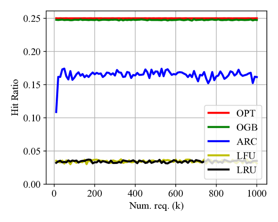
Figure 1: Adversarial trace: comparison of different cache policies. While traditional recency or frequency based policies are not able to cope with adversarial patterns, the OGB policy show a close-to-optimal performance.

This simple example of adversarial trace shows the limits of known policies, which work for a specific arrival pattern, but not in the general case. The example shows that indeed LRU and LFU policies have linear regret (the difference of the cumulative number of hits between OPT and LRU or LFU grows linearly with the number of requests), which was theoretically proved in [23].

Real-world (short) trace. The adversarial setting may be considered unrealistic. In Figure 2 (top), we consider then a real-world trace for which LRU works reasonably well. We observe that OGB’s regret guarantees translate in practice in a robustness to deviations in the request process, so that also OGB policy obtains a high hit ratio, even higher than LRU. This trace contains $10^{5}$ requests for $10^{4}$ items (cache size $C=500$ items) and it has been subsampled from the publicly available trace from [30, 35], to generate a trace comparable, in terms of catalog size and number of requests, with the traces considered in previous works (see Table 1).

The OGB scheme has a parameter, the learning rate $\eta$, and the figure shows that OGB has a limited sensibility to such a parameter. For comparison, we consider another policy with sub-linear regret guarantees called Follow The Perturbed Leader (FTPL) [1], which is a variant of the Follow The Leader (FTL) policy with the addition of a Gaussian noise. When applied to our caching problem, FTL coincides with LFU and can be proved to have linear regret [23]. Interestingly, FTPL, by adding a noisy random variable to each item counter achieves sublinear regret [1]. The noise is normally distributed with zero mean and standard deviation $\zeta=\frac{1}{(4\pi\log N)^{1/4}}\sqrt{\frac{T}{C}}$. In Figure 2 (bottom) we see that this policy is much more sensible to the variability of the parameter $\zeta$.

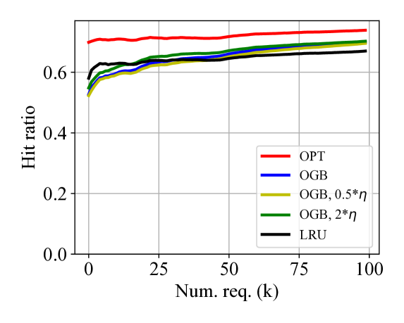
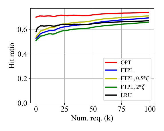
Figure 2: Real-world short traces: sensitivity of OGB and FTPL. In OGB, the parameter $\eta$ is the learning rate, while in FTPL the parameter $\zeta$ is the noise added to the LFU counters.

Computational complexity. The main issue with the OGB policy is its computational complexity. While common cache policies have $\text{O}(1)$ or $\text{O}(\log C)$ complexity per request ($C$ is the cache size), the best known implementations of OGB have $\text{O}(N)$ complexity per request [28]. This high complexity has limited the adoption of OGB policies and their experimental validation. Table 1 shows the most recent works on sub-linear regret policies in the context of caching, with the catalog size and the trace length. In all the cases, the tests have been conducted on catalogs that are order of magnitude smaller than those typical of real-world cases. The same is true for the trace length, with the only exception of [21], which considers a real-world trace publicly available trace, but selects only a subset of the catalog (with $10^{4}$ items).

Table 1: Catalog size ($N$) and trace length ($T$) used in the literature. The high computational complexity limit the settings for testing low regret policies.

Paper	Year	N	T
Paschos et al. [23]	2019	$10^{4}$	$2\cdot 10^{5}$
Bhattacharjee et al. [1]	2020	$4\cdot 10^{3}$	$10^{5}$
Paria et al. [21]	2021	$10^{4}$	$1.5\cdot 10^{6}$
Mhaisen et al. [16]	2022	$10^{4}$	$5\cdot 10^{3}$
Mhaisen et al. [17]	2022	$10^{4}$	$10^{4}$
Si Salem et al. [28]	2023	$10^{4}$	$1.5\cdot 10^{5}$

Open issues. Without a low complexity implementation of OGB, this policy is likely to remain a theoretical exercise with no practical interest. To the best of our knowledge, there are no work that proves that OGB works well with large catalogs and long traces that have heterogeneous patterns.

The only low complexity sub-linear regret policy is a variant of FTPL. In its original design [1], the noise is added at each request, and therefore the counters need to be re-sorted, with a $\text{O}(N\log N)$ complexity per request. Instead, in the variant suggested, among others, by Mhaisen et al. [17], we can add an initial noise to each item, without changing it at every request. This lowers the complexity to $\text{O}(\log N)$ per request (ignoring the initial sorting) due to the maintenance of the ordered data structure. Despite the fact that the FTPL policy is equivalent to LFU with some initial noise—and therefore it has the same limitation of LFU—this policy has a high sensibility to the variation of its parameter. This is confirmed also in case of a long trace—see Figure 3, bottom, in which the catalog has $6.8\cdot 10^{6}$ items and $35.2\cdot 10^{6}$ requests (the details of the trace are described in Sec. 6).

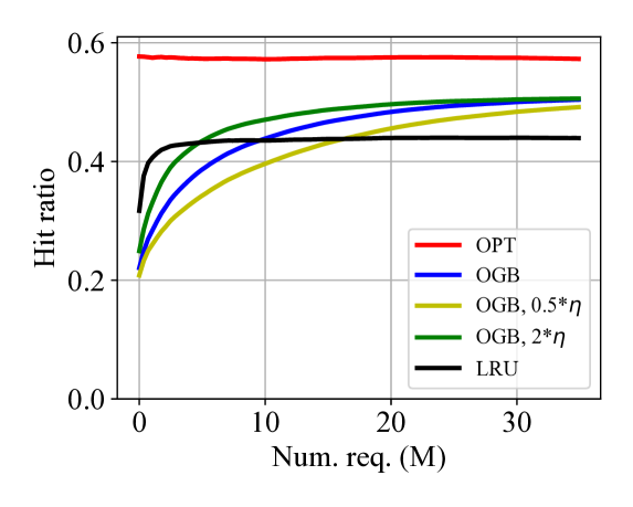
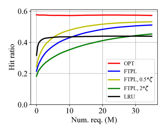
Figure 3: Real-world long traces: sensitivity of OGB and FTPL. The initial noise added by FTPL heavily influences the perfomance.

Figure 3, top, shows indeed that OGB is able to provide low regret performance with real-world traces that contains millions of requests for a large catalog, and its sensitivity to the learning parameter is limited. These results have been made possible thanks to our solution, which has $\text{O}(\log N)$ computational complexity, which is the core contribution of this work.

2.3 Applications beyond caching

Paschos et al. [23] were the first to frame the caching problem as an optimization problem, and therefore adopted a set of tools and algorithms from the online learning literature.

Online learning is a fundamental paradigm for modeling sequential decision making problems [27]. In such a setting, there are a learner and an adversary that play repeatedly. In each round, the learner has to make a selection among $N$ possible choices. Then the adversary reveals an arbitrary assignment of losses (or gain) to the choices and the learner suffers a loss (or obtain a gain) on the choice she made.

While in some cases the dimensionality of the problems that can be represented as an online learning problem may allow the use of algorithms with linear complexity, in other cases, such as in [4], the number of choices is very large, and there is an increasing interest in finding efficient algorithms for solving these problems [10, 32].

Currently, the most efficient implementations are based on variants of the FTPL [11, 5, 10, 32]. To the best of our knowledge, no online gradient based solution has been proposed in this context. Given the issues with FTPL that we highlight in the previous paragraphs (see also Sec. 6 for additional results), our efficient solution could be relevant not only for caching, but also for other online learning problems.

3 Solution overview

The cache state $\bm{x}_{t}$ indicates which of the $N$ items are stored in the cache. Our scheme is based on the OGB policy, therefore we maintain a vector $\bm{f}_{t}$ where we store, for each item, the probability that such an item is cached at time slot $t$. Intuitively, if an item is requested repeatedly, such a probability should increase, while, if an item is not requested, its probability should decrease. This is fundamentally different from policies like LFU and FTPL, which accumulate the number of requests for each item and base their choices on this information, without adjusting the counters for non-requested items.

The solution we propose is composed by two steps (see Figure 4. At each time slot $t$, when a new request arrives, (i) we update $\bm{f}_{t}$ while maintaining the constraints on the feasibility of the fractional state space, and (ii) we update $\bm{x}_{t}$ based on the current value of $\bm{f}_{t}$. In the notation, if it is clear from the context, we sometimes avoid using the indication of the time slot $t$.

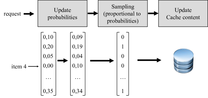
Figure 4: High level view of the building blocks that compose the solution: the item selection passes through the computation of the caching probabilities.

Update (projection). The update of the vector $\bm{f}_{t}$ is an optimization problem known as projection onto the capped simplex [33]. When a new request arrives, we have a vector $\bm{y}_{t}$ which is derived from the current $\bm{f}_{t}$ and include the modification of the component related to the requested item, i.e., $\bm{y}_{t}=\bm{f}_{t}+\eta\nabla\phi(\bm{f}_{t})$. Since $\sum_{i=1}^{N}y_{t,i}>C$, we should compute the new version of $\bm{f}_{t+1}$ by projecting $\bm{y}_{t}$ on a feasible state, i.e., $\bm{f}_{t+1}=\Pi_{\mathcal{F}}\left(\bm{y}_{t}\right),$. where $\Pi_{\mathcal{F}}(\cdot)$ is the solution of the following minimization problem:

$$\min_{\bm{f}\in\mathbb{R}^{N}} \frac{1}{2}\lVert\bm{f}-\bm{y}\rVert^{2}\quad\quad\textrm{s.t.}\quad 0\leq\bm{f}\leq 1,\quad\sum_{i=1}^{N}f_{i}=C.$$ (2)

For the general case in which more than one component of $\bm{y}$ has changed with respect to the current $\bm{f}$, the best known algorithm has $\text{O}(N^{2})$ complexity [33]. In case of there is a single component that changes with respect to the current $\bm{f}$, Paschos et al. [23] propose a $\text{O}(N\log N)$ complexity solution. In the context of caching, with OGB, the single request modifies a single component of $\bm{f}$, therefore we design a scheme for this case that has $\text{O}(\log N)$ complexity.

Selection. Once we have updated $\bm{f}$, we should select which items should be stored in the cache. In doing this, we should maximize the overlap of the selected items (current and previous cache state). In LRU, for instance, at most one item is added and another item is removed, which has a limited impact on the amount of data exchanged between the cache and the origin server.

A naïve solution to this problem is to consider each item independently and select them according to their probability $f_{i}$. Not only does this approach have $\text{O}(N)$ complexity, but it does not guarantee to select exactly $C$ items, nor does it minimizes the items changed in the cache—from one update to the next it could replace all the items.

In order to select exactly $C$ items, it is possible to adopt a systematic sampling approach devised by Madow et al. [9]. Despite being an elegant solution to a complex issue, it still requires $\text{O}(N)$ operations and it does not guarantee to minimize the changes in the cache, although experimental evidence shows that indeed the number of replaced items is small [28].

By formulating the problem as a optimal transport problem, we can guarantee to select exactly $C$ content and limit the number of replacements, but this can be done with a high computation cost, i.e., with $\text{O}(N^{3})$ complexity [24].

Overall, it is not possible to provide these three desired properties—selection of exactly $C$ items, minimization of the replacements, and low complexity solution—at the same time. By relaxing the constraint on the exact number of items, we are able to design a scheme that minimizes the number of replaced items with a $\text{O}(\log N)$ complexity.

Overall complexity and regret guarantees. By combining the two steps described above, since each step has $\text{O}(\log N)$ complexity, we provide a solution whose complexity is comparable to well known and widely used caching policies, making it a practical policy that can be readily adopted with no assumption on the request arrival pattern.

The definition of the OGB scheme is equivalent to the one provided in [23], therefore the regret guarantees comes from this equivalence. In addition, Si Salem et al. [28, Prop. 6.2] shows that the integral caching, in which the item selection follows a randomized scheme guided by the items probabilities, maintains the regret guarantees of the policy that generated the items probabilities. Overall, our solution represent an efficient OGB caching policies with sub-linear regret.

Table 2: Notation Summary

Notation	Description
$\mathcal{N}$	Catalog set with size $|\mathcal{N}|=N$
$C$	Cache size
$\mathcal{X}$	Set of integral states
$\mathcal{F}$	Set of fractional states
$\bm{x}_{t}$	Cache state at time slot $t$
$\bm{x}^{*}$	Optimal cache allocation in hindsight
$\bm{f}_{t}$	Caching probability at time slot $t$
$\tilde{\bm{f}}$	Caching probability, not adjusted
$\rho$	Global adjustment factor to apply to $\tilde{\bm{f}}$
$\bm{y}_{t}$	Temporary probability to be projected
$\mathcal{M}_{p}$	Set of positive components of $\bm{y}_{t}$
$T$	Time horizon
$\eta$	Learning rate for OGB policy
$\zeta$	Perturbation in FTPL policy
$\bm{r}$	Permanent Rand. Numb. assigned to the items

4 Projection onto the Capped Simplex

The caching strategy should increase the probability of a requested item while decreasing the probabilities of the others. These two operations are indeed accomplished in two different steps by the OGB policy. First, we increment the component related to the requested item by a value equal to the step size $\eta$. The gradient $\nabla\phi(\bm{f}_{t})$ in Eq. (1), in fact, is $w_{t,j}$ for the requested item $j$, and, even if our solution works for any $w_{t,j}$, to simplify the description we consider the case $w_{t,j}=1$. Then, the projection $\Pi_{\mathcal{F}}(\cdot)$ decreases all the components, such that their sum is equal to $C$. In order to design a low complexity algorithm, we need to understand how the projection actually operates.

From a starting projection $\bm{f}_{t}$, when item $j$ is requested, we obtain the following vector $\bm{y}_{t}$:

$$y_{t,i}=\begin{cases}f_{t,i}&\text{if }i\neq j,\\ f_{t,i}+\eta&\text{if }i=j.\end{cases}$$

Clearly we have $\sum_{i=1}^{N}y_{t,i}=C+\eta$ and the aim of the projection is to remove the excess $\eta$. Let $\mathcal{M}_{p}=\{y_{t,i}:y_{t,i}>0\}$ be the set of positive components of $\bm{y}_{t}$. In order to minimize the squared norm in Eq. (2), the excess should be uniformly taken from each positive component. Let $\rho=\eta/|\mathcal{M}_{p}|$, then the projection $\bm{f}_{t+1}$ would be:

$$f_{t+1,i}=\begin{cases}y_{t,i}-\rho&\text{if }y_{t,i}\in\mathcal{M}_{p},\\ 0&\text{otherwise}.\end{cases}$$

Note that the set $\mathcal{M}_{p}$ contains also the item $j$ that has been requested. As an example, in Fig. 5 we show a small vector with six components. The initial state is represented by the blue bars. When a new request for item 1 arrives, we first add the orange contribution to component 1. We then uniformally decrease all the components (and obtain the green bars) such that the sum of all the components remains constant. Since we need to ensure that all the components of projection falls within the range [0,1], there are some corner cases that need to be considered.

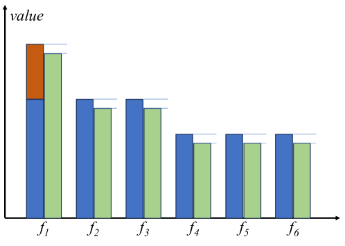
Figure 5: Example of a projection on a small vector. Starting from a feasible solution (blue bars), a new request for item 1 generates an excess (orange bar), which is taken evenly from all the components (green bars) to obtain a new feasible solution.

The first case is when the component related to the requested item $j$ goes above one, i.e., $f_{t,j}\leq 1$, but $f_{t,j}+\eta-\rho>1$. This case is easy to manage, by modifying the excess to redistribute to $\eta^{\prime}=\eta-(f_{t,j}-1)$. The component $f_{t+1,j}$ is set to one, and $\mathcal{M}^{\prime}_{p}=\mathcal{M}_{p}\setminus\{j\}$. Note that, in the trivial case $f_{t,j}=1$, the $j$-th component of $\bm{y}_{t}$ becomes $y_{t,j}=1+\eta$ and the final projection is simply $\bm{f}_{t+1}=\bm{f}_{t}$.

The second case is when a component becomes negative, i.e., $y_{t,i}>0$, but $y_{t,i}-\rho<0$. This changes the set $\mathcal{M}_{p}$ and the excess to be redistributed: in particular, $\eta^{\prime}=\eta-\{y_{t,i}:y_{t,i}-\rho<0\}$ and $\rho^{\prime}=\eta^{\prime}/|\mathcal{M^{\prime}}_{p}|$.

While these corner cases require some attention, the main observation remains: the projection, in its essence, is a uniform redistribution of some excess. This aspect can be exploited in the design of a low complexity algorithm for the update of the projection.

4.1 Improving Projection: Main Idea

Consider two items, $a$ and $b$, with $f_{a}>0$ and $f_{b}>0$. Assume that they are not requested during two consecutive requests. After the first request, their values are decreased by the same quantity $\rho_{1}$. After the second request, their value are decreased by the same quantity $\rho_{2}$. If, during the update, we do not fall into the corner cases, i.e., $f_{a}-\rho_{1}-\rho_{2}>0$ and $f_{b}-\rho_{1}-\rho_{2}>0$, we do not need to actually update the two components, but we can maintain an external variable $\rho=\rho_{1}+\rho_{2}$ and we know that the projection of the components $f_{a}$ and $f_{b}$ are indeed $f_{a}-\rho$ and $f_{b}-\rho$.

To manage the corner cases, we need to detect when a component goes below zero. To this aim, we keep a copy of the (positive components of the) vector $\bm{f}$ sorted by the component values. When we update $\rho$ to a new value $\rho^{\prime}$, we check which components are smaller than $\rho^{\prime}$, remove them and adjust $\rho^{\prime}$. When a request for item $j$ arrives, we update the corresponding value in $\bm{f}$ and in the sorted copy, considering the recently computed value of $\rho$. In this way, for the all the positive components, we can derive the current projection from $\bm{f}$ and $\rho$.

Managing the sorted copy of the coefficients has $\text{O}(\log N)$ complexity. Clearly, if we need the actual projection for all the components, then we have to update each coefficient. This means that any algorithm that, at each step, actually updates the projection, can not have complexity less than $\text{O}(N)$. But in our case, since the projection is used to select the item to cache, we do not need to actually update all the components, but we only need to know which components falls below a threshold—we defer to Sec. 5 for a detailed explanation of this aspect.

4.2 Improving Projection: The Algorithm

The proposed algorithm is based on the fact that the projection is a constrained quadratic program and the objective function is strictly convex with a unique solution characterized by its KKT system [19]. As done in [33] and [23], we look at the set of coefficients that are respectively greater than one, between zero and one, and zero, and we adjust them with with the uniform redistribution of the excess.

input :  $\bm{\tilde{f}}$, current state

input :  $\rho$, current adjustment

input :  $\bm{z}$, ordered tree with pos. coeffs. of $\bm{\tilde{f}}$

input :  $j$, index of the requested item

input :  $\eta$, OGB step size

1

// The requested item is already 1

2 if $\tilde{f}_{j}-\rho==1$ then

3       return;

4      

// The requested item was 0

5 if $\tilde{f}_{j}==0$ then

6       $\tilde{f}_{j}\leftarrow\rho+\eta$;

7       $z_{j}\leftarrow\rho+\eta$;

8       $\bm{z}\leftarrow\bm{z}\cup\{z_{j}\}$;

9      

10else

       // Update with the OGB step

11       $\tilde{f}_{j}\leftarrow\tilde{f}_{j}+\eta$;

12       $z_{j}\leftarrow z_{j}+\eta$;

13      

14

// Remove items with negative values

15 $\eta^{\prime}=\eta$;

16 repeat

17       $\rho^{\prime}=\eta^{\prime}/|\bm{z}|$;

18       $\mathcal{B}\leftarrow\emptyset$;

19       $\mathcal{B}\leftarrow\{i:z_{i}-\rho-\rho^{\prime}<0\}$ ;

20       $\eta^{\prime}\leftarrow\eta^{\prime}-z_{i},\quad\forall i\in\mathcal{B}$;

21       $\bm{z}\leftarrow\bm{z}\setminus\{z_{i}:i\in\mathcal{B}\}$ ;

22       $\tilde{f}_{i}\leftarrow 0,\quad\forall i\in\mathcal{B}$ ;

23      

24until $\mathcal{B}$ is empty;

// Check the largest value

25 $z_{max}\leftarrow\max\bm{z}$;

26 if $z_{max}-\rho>1$ then

27       $\eta^{\prime}=\eta-(z_{max}-1)$;

28       $\bm{z},\bm{\tilde{f}}\leftarrow$ RestoreRemoved$()$;

29       $\bm{z}\leftarrow\bm{z}\setminus\{z_{max}\}$ ;

30       $\tilde{f}_{i}\leftarrow 1,\quad i$ index of $z_{max}$ ;

31       GoTo line 1;

32      

33else

34       $z_{max}\leftarrow 0$;

35      

// Update $\rho$

36 $\rho\leftarrow\rho+\rho^{\prime}$;

37 if $z_{max}>0$ then

38       $z_{max}\leftarrow z_{max}+\rho^{\prime}$;

39       $\bm{z}\leftarrow\bm{z}\cup\{z_{max}\}$ ;

40       $\tilde{f}_{i}\leftarrow\tilde{f}_{i}+\rho,\quad i$ index of $z_{max}$ ;

41      

Algorithm 1 Projection update

Differently from the above mentioned papers, following the ideas presented in Sec. 4.1, we maintain an ordered data structure $\bm{z}$, which contains the positive coefficients of the vector $\bm{\tilde{f}}$, and an external adjustment coefficient $\rho$. After any projection update, we can obtain the actual value of each component of $\bm{f}$ with:

$$f_{i}=\begin{cases}\tilde{f}_{i}-\rho&\text{if }\tilde{f}_{i}>0,\\ 0&\text{otherwise}.\end{cases}$$

When a new request for item $j$ arrives, we first check if $f_{j}$ is already equal to one, in which case there is no update. Otherwise, we assign the step size $\eta$ to the component $j$. If $f_{j}$ was equal to zero, we adjust its value considering the current adjustment coefficient $\rho$.

The next two blocks—lines 1–1 and lines 1–1—deals with the two corner cases, in which the redistribution of the excess produces negative coefficients or a coefficient greater than one. As already observed in [19], there could be at most one coefficient greater than one at each request, because only one component is incremented at each request, while all the other positive components are decremented. As for the components that become negative, on average there is at most one such component, since in the worst case an adversarial request pattern keeps changing requested items. Intuitively, even if some group of items have similar values, in one single update those group may be removed, but such an event will be followed by many updates in which no component becomes negative. In particular, we can prove that on average a single element will be set equal to 0 after each request. Indeed, consider the cache after the first $t$ requests. At any time, there can be at most $N-C$ components of the vector $\bf{f_{t}}$ equal to 0. Moreover, at each request, there can be at most one component which turns positive (because the corresponding item has been requested). It follows that the total number of components set to $0$ over the $t$ requests is upper-bounded by $N-C+t$. Then, on average $1+\frac{N-C}{t}$ new components are set to $0$ at each request, and the average time complexity of the cycle at lines 1–1 is $\mathcal{O}(1)$. In practice, in our experiments we observe that the loop is executed at most two consecutive times per request, as also observed in [23, IV.B]. The time-complexity of projection update is then determined by the need to keep the data structure ordered, which is $\mathcal{O}(\log N)$.

5 Cache Content Update

After each request, the cache may change the set of items cached locally. In the literature, this is usually referred to as a rounding scheme [21, 28], since the fractional state $\bm{f}_{t}$ with continuous components between $0$ and $1$ is mapped to a caching vector $\bm{x}_{t}$ whose components are either zero (the item is not cached) or one (the item is cached).

The selection can be seen as a sampling process, in which the probability that an item $i$ belongs to the sample is proportional to its component $f_{i}$. Considering the sampling literature, this is known as probability proportional to size (PPS) sampling.

Problem definition. Since $\bm{f}$ varies as new requests arrive, we are interested in finding a scheme that, starting from the previous sample, and considering the updated $\bm{f}$, create a new sample that has a large overlap with the previous one. Sample coordination refers to the process of adjusting the overlap between successive samples [31]. With positive coordination the number of common items between two consecutive samples is maximized, while with negative coordination this number is minimized. We aim at finding a positive coordination design that is computationally efficient.

Current solutions. PPS sampling schemes that provide an exact number of samples—such as systematic sampling used in [21, 28]—have at least $\text{O}(N)$ complexity. To the best of our knowledge, there is no extension of systematic sampling to successive sampling, therefore the only option is to re-apply the scheme from scratch. This does not guarantee to maintain the same set of items over successive samples.

Any scheme that aims at maximizing the overlap of successive samples with an exact sample size, requires the computation of joint inclusion probabilities over subsequent samples, which in turn involves an update on every pair of items [31], so it has at least $\text{O}(N^{2})$ complexity.

Our approach. By allowing the sample size to fluctuate around the exact cache size, we can design a low-complexity scheme with a tunable sample coordination.

5.1 Coordination of Samples

First sample. The components of $\bm{f}$ satisfy the following constraints: $0\leq f_{i}\leq 1,\forall i\in\mathcal{N}$, and $\sum_{i=1}^{N}f_{i}=C$. Therefore, we can apply Poisson sampling [20], i.e., we decide to include an item in the sample independently from the other items. To this aim, we associate a random number $r_{i}$, drawn from a uniform distribution between zero and one, to each item $i$, and we include the item $i$ in the sample if and only if $r_{i}\leq f_{i}$. The resulting sample has a random sample size with expectation $C$, the cache size. With sufficiently large $C$ the variability around the expectation is limited. In particular, the variability is the largest when each item has the same probability to be stored in the cache, i.e., $f_{i}=C/N$ for each $i\in\mathcal{N}$. Considering this setting, the coefficient of variation (the ratio between the standard deviation and the expected value) for the number of items sampled can be easily upper-bounded by $1/\sqrt{C}$. It is then smaller than 1% as far as $C\geq 10000$. Moreover, the Gaussian approximation allows us to bound the probability that the number of items sampled exceed by $\epsilon C$ the average cache size $C$ is upperbounded by $\Psi(\epsilon\sqrt{C})$, where $\Psi(\cdot)$ is the complementary cumulative distribution function of a standard normal variable. This allows us for example to conclude that in the same setting, the probability that the instantaneous cache occupancy may exceeds $C$ by more than $3\%$ with probability smaller than 0.13%. Theorem 1 in [6] presents a similar result based on Chernoff bound.

Subsequent samples. Brewer et al. [2] showed that Poisson sampling can be used for coordination by letting $r_{i}$ to be the permanent random number associated to item $i$. As $f_{i}$ changes over time—let $f_{t,i}$ the value at time slot $t$—the sample selection rule remains the same: the item is included as long as $r_{i}\leq f_{t,i}$. It is possible to introduce a rotation in the sample by changing randomly a subset of the random numbers assigned to the items [20].

Putting the pieces together. In Sec. 4 we proposed a scheme in which, rather than computing $f_{i}$ at every request, we update the global adjustment $\rho$, along with $\tilde{f}_{i}$ if item $i$ has been requested, knowing that $f_{i}=\tilde{f}_{i}-\rho$. After an update, we need to check which items needs to be included or evicted from the cache. The items can be divided into three groups.

The first group includes only the item that has been requested. If it was already cached, since $f_{i}$ increased, it continues to be cached. If it was not cached, we simply need to check that $f_{i}\geq r_{i}$, i.e., $\tilde{f}_{i}-\rho\geq r_{i}$.

The second group contains the items that have not been requested and were not in the sample: since $f_{t+1,i}<f_{t,i}$, the items continue to stay out of the sample, i.e., we do not need to manage all the items not cached and not requested.

The third group includes all the cached items (excluding the requested one, if it was cached). In this case we need to check if, for some item, $f_{i}$ became smaller than $r_{i}$, i.e.,

$$\tilde{f}_{i}-\rho<r_{i}.$$

For these items, both $\tilde{f}_{i}$ and $r_{i}$ remained unchanged, only $\rho$ has been updated. Therefore, the previous check can be rewritten as

$$\tilde{f}_{i}-r_{i}<\rho.$$

The key observation is that, at every update, for all the cached items (except the single item that has been requested, if it was cached), the difference $d_{i}=\tilde{f}_{i}-r_{i}$ remains constant. Therefore we can put the values of $d_{i}$ in an ordered data structure and check which items has $d_{i}<\rho$ as $\rho$ changes from one update to the next.

5.2 Item selection: The algorithm

Algorithm 2 summarizes the operation at each request arrival. The only new item that could be potentially added to the cache is the requested one (lines 2-2). As for the eviction (lines 2-2), the ordered data structure $\bm{d}$ allow us to reach the first elements smaller than the current value of $\rho$ with $\text{O}(\log N)$ complexity. After that, since the leaves of the tree are chained together, we can remove all the items with $d_{i}<\rho$.

input :  $\bm{\tilde{f}}$, current fractional state

input :  $\bm{x}$, current cache state

input :  $\rho$, current adjustment

input :  $\bm{r}$, permanent random numbers

input :  $\bm{d}$, ordered tree with differences $(\tilde{f}_{i}-r_{i})$

input :  $j$, index of the requested item

1

// Manage the requested item

2 if $j$ index in $\bm{d}$ then

3       $d_{j}\leftarrow(\tilde{f}_{j}-r_{j})$;

4      

5else

6      if $\tilde{f}_{j}-\rho\geq r_{j}$ then

7             $d_{j}\leftarrow(\tilde{f}_{j}-r_{j})$ ;

8             $\bm{d}\leftarrow\bm{d}\cup\{d_{j}\}$;

             // Add the item to the cache

9             $x_{j}=1$;

10            

11      

// Eviction

12 $x_{i}=0,\quad\forall i:d_{i}<\rho$;

13 $\bm{d}\leftarrow\bm{d}\setminus\{d_{i}:d_{i}<\rho$} ;

Algorithm 2 Item selection update

Since Algorithm 2 uses the current value of $\rho$ to evict the content, we would like to stress again the fact that we do not need to compute $f_{i}$ for all the items, but it is sufficient to update $\bm{\tilde{f}}$ with the requested item, which is done by Algorithm 1.

Finally, Algorithm 2 does not modify the permanent random numbers associated to the items. If we would like to stochastically refresh the cache content, we can change a fixed number of permanent random numbers, e.g., 10, following a random permutation of the indexes of the catalog, such that, after a given number of requests, all $r_{i}$s have been changed. When $r_{i}$ is changed, we simply update the value of $d_{i}$ and the decision about its cacheability.

5.3 On the fractional case

The previous step allows us to obtain, starting from the selection probabilities of each item, a sample with a set of desired properties. In case of fractional caching, at time slot $t$ we maintain in the cache the chunks for all the items with $f_{t,i}>0$ (recall that $\sum_{i=0}^{N}f_{t,i}=C$, the cache size). When $\bm{f}$ is updated, all the components greater than zero are modified: the component corresponding to the requested item increases, while all the others decrease. This, in practice, means that a new portion of the requested item is cached, while small portions of the non-requested items are removed. The fractional case, therefore, has an intrinsic $\text{O}(N)$ complexity.

Algorithm 1 has $\text{O}(\log N)$ complexity when it computes the adjustment factor $\rho$ and it manages the corner cases. The knowledge of the updated $\rho$ is used by Algorithm 2 for the sampling, without the need to compute the actual values of $\bm{f}_{t}$. But in the fractional case we need $\bm{f}_{t}$, therefore we need to run through all the components of $\tilde{\bm{f}}_{t}$.

In order to limit the cost of maintaining $\bm{f}_{t}$, we can delay the updates after having received a batch of requests [28]. The fractional cache state $\bm{f}_{b}$ remains the same for $B$ requests, i.e., we receive a gain $\sum_{i=1}^{N}q_{t,i}f_{b,i}$, with $t=t_{1},t_{1}+1,t_{1}+2,\ldots,t_{1}+B$ and $b$ fixed. At the same time, we update $\tilde{\bm{f}}_{t}$ and $\rho$. Once the batch is completed at $t_{2}=t_{1}+B$, we compute the new fractional state $\bm{f}_{b+1}=\tilde{\bm{f}}_{t_{2}}+\rho$ and we update the cache elements according to the new $\bm{f}_{b+1}$.

Overall the scheme has $\text{O}(N/B)$ complexity. The adoption of batches introduces a trade-off. As $B$ increases, we update less often $\bm{f}_{b}$, and reduce the practical computational cost. At the same time, the gain we obtain comes from a cache that is updated every $B$ requests, so we may miss opportunities for hits. From the theoretical point of view, it is interesting to note that the sub-linear guarantees are still confirmed [28].

6 Experiments

The low complexity of our solution allows us to test the OGB caching policy on traces with millions of requests and millions of items, an accomplishment that previous works could not achieve. We consider a set of real-world representative cases, but we stress the fact that the sub-linear regret obtained by the OGB policy is guaranteed by the theoretical results. The aim of the measurement campaign is then to explore different scenarios.

Our main reference for the comparison is the optimal static allocation in hindsight (OPT), which is the policy for which the regret metric has been defined. As a baseline, we consider LRU, which, depending on the traffic pattern, may obtain good performances. Due to the computational complexity of previously proposed no-regret policies, we can not test them we the traces we consider. The only exception is the FTPL policy with the noise added only at the beginning, but this policy has the issues highlighted in Sec. 2, and we show other cases in which these issues occur.

6.1 Traces

We consider a set of publicly-available block I/O traces from SNIA IOTTA repository [29], a Content Delivery Network (CDN) trace from [30, 35], and the Twitter production cache traces from [34, 36]. Table 3 summarizes the characteristics of the traces. From the SNIA IOTTA repository, we have considered the most recent trace—labeled as systor [13]—along with older traces collected at Microsoft [12], labeled as ms-ex. The cdn trace refers to a CDN cache serving photos and other media content for Wikipedia pages (21 days, collected in 2019). The twitter trace considers their in-memory cache clusters and have been collected in 2020.

Table 3: Trace characteristics: catalog size ($N$) and trace length ($T$)

name	year	$\bm{N}$	$\bm{T}$	reference
ms-ex	2007	$2.6\cdot 10^{6}$	$8.9\cdot 10^{6}$	[12]
systor	2016	$6.8\cdot 10^{6}$	$19.3\cdot 10^{6}$	[13]
cdn	2019	$6.4\cdot 10^{6}$	$35.2\cdot 10^{6}$	[30]
twitter	2020	$2.7\cdot 10^{6}$	$20.0\cdot 10^{6}$	[34]

Note that the full traces sometimes contain different subtraces, and each subtrace may include hundreds of millions of requests over several days. In our experiments, we consider mostly the subtraces related to Web content or e-mail servers – the only exception is the systor trace, which considers storage traffic from a Virtual Desktop Infrastructure.

For experimental reproducibility, we report here the details of the subtrace we use. The ms-ex is the trace taken from [12] named “Microsoft Enterprise Traces, Exchange Server Traces,” which have been collected for Exchange server for a duration of 24-hours – we consider the first 3.5 hours. The systor traces [13] collect requests for different block storage devices over 28 days: we consider 12 hours(March, 9th) of the device called “LUN2.” The cdn trace contains multiple days of traffic, of which we consider portions of 6 hours – we tested different intervals finding similar qualitative results. Finally, for twitter we considered the first 20 millions requests from cluster 45. Also in this case, we obtained similar qualitative results for other clusters.

6.2 Results

The main metric of interest is the hit ratio, i.e., the ratio between the number of hits and the number of requests. Usually, given a trace, the computation takes into consideration the cumulative number of hits and requests—this is also what we show in the results anticipated in Sec. 2. Since the traffic pattern may change over time, the cumulative representation may smooth such variability. For this reason, in this section we present the hit ratio computed over non-overlapped windows of $10^{5}$ requests, i.e., each point in the graph represents the number of hits in the last $10^{5}$ requests, divided by $10^{5}$. If not otherwise stated, the cache size is set to 5% of the catalog size.

Figure 6 shows the results for the less recent traces, ms-ex and systor. In both cases, we can observe a highly variable hit ratio over time for the OPT policy. Both LRU and OGB are able to follow such variability. In the ms-ex trace, the OGB policy takes some time to reach the optimal hit ratio: the regret guarantees are provided at the end of the horizon $T$, so it may take some time for the policy to converge. In other cases, such as the systor traces, this convergence is faster.

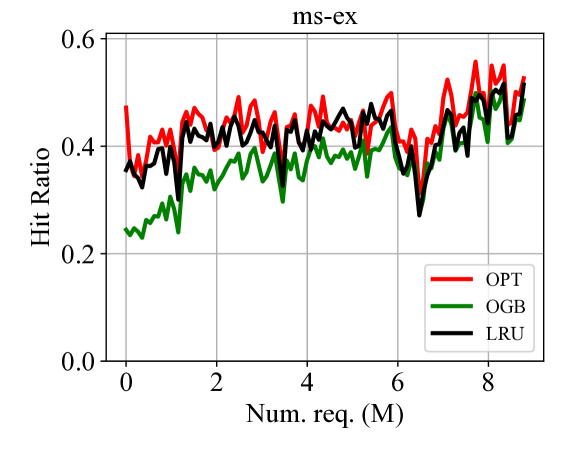
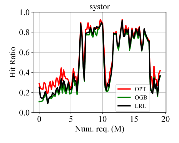
Figure 6: Real-world long (less recent) traces: Performance of OGB policy.

A similar behaviour, in which it takes some time for OGB policy to converge, appears in the cdn trace (Fig. 7, top). Here the traffic pattern is much more stable, and the gap between LRU and OPT is more evident. The twitter trace shows an interesting scenario, in which the LRU policy is able to beat the OPT policy (Fig. 7, bottom).

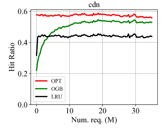
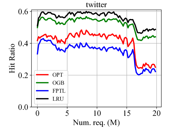
Figure 7: Real-world long (more recent) traces: Performance of OGB policy.

In this case, the traffic pattern favors recency-based policies such as LRU over frequency-based one—OPT is a static allocation of the most requested items in the trace. The OGB policy follows LRU and improves over OPT. In this scenario, we consider the FTPL policy, testing different values of its parameter $\zeta$. In Fig. 7, bottom, we show the best result FTPL can achieve: since it is a frequency-based policy, its performance are comparable, at best, to the OPT policy results.

Other statistics. The sampling scheme we adopt does not guarantee to have exactly $C$ items in the cache. To understand the variability in the number of store items, we record at regular intervals the cache occupancy. Figure 8, top, shows the percentage of items stored in the cache with respect to the nominal cache size. Since we have traces with different lengths, we normalized the x-axis with respec to the trace length. In all cases, the variability is limited to 0.5% the cache size. Therefore, when suing this scheme, we need to provide a limited extra storage with respect to the nominal size we use in the scheme.

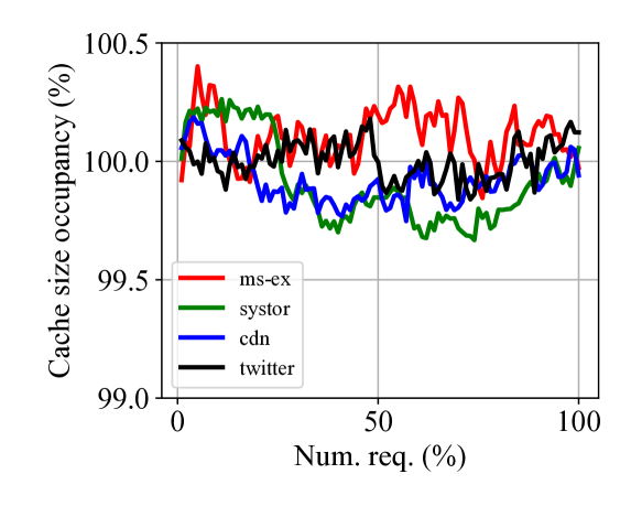
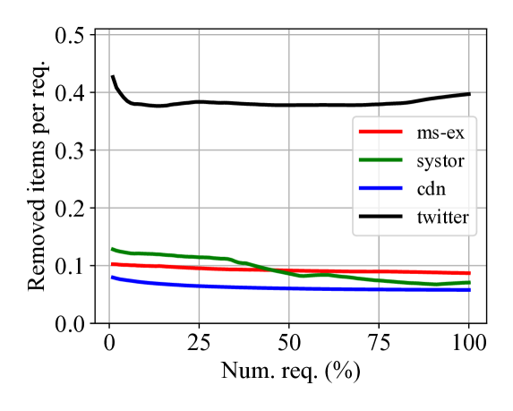
Figure 8: Cache occupancy over time (top) and average removed items per request (bottom).

Figure 8, bottom, shows the number of items that are removed from $\tilde{\bm{f}}$ in Algorithm 1. We consider windows of $10^{5}$, and we record the number of removed components (lines 1–1), then normalize the value with the window size. In all cases we are below 0.5 removed items per requests, confirming the analysis provided at the end of Sec. 4.

6.3 Fractional case

We consider the fractional case presented in Sec. 5.3, in which the cache can store any fraction of each item. In order to limit the computational complexity, we materialize the cache choices every $B$ requests, and the hits are recorded considering the current cache state.

Figure 9 shows the impact of $B$ for the cdn and twitter traces. As observed in the in the previous section, the arrival pattern in these two cases is very different: in the cdn trace the pattern is more regular, while in the twitter trace the temporal locality is more pronounced. This is confirmed also by looking at the impact of $B$.

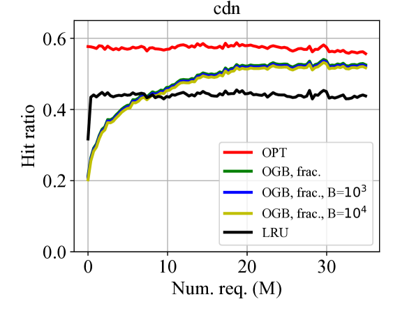
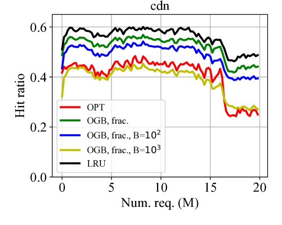
Figure 9: Real-world long traces: Performance of OGB policy in the fractional case for variuos values of the batch size $B$.

In the cdn trace, even large values of $B$ do not affect the performance, since the items are repeatedly requested over time and the cached portions generates hits. In the twitter trace, since the cache is renovated more often, stale cached items limit the hit ratios. In general, therefore, it is not possible to understand how much the computational complexity can be decreased, since the actual value of $B$ depends on the trace characteristics.

7 Related work

The caching problem has been extensively studied in the literature. Since our work concern the efficient implementation of a policy with specific characteristics, we discuss here the literature considering these aspect.

Well known caching policies, such as LRU, LFU [14], FIFO [7] and ARC [15] are widely adopted due to their constant complexity: at each new requests they update the cache in $\text{O}(1)$ steps. In some contexts where the arrival rate is extremely high and the speed of the cache is a key issue, these policies are the only viable solution. The price paid is represented by their performance in terms of hit ratios. Since these policies works well with specific traffic patterns, they can not provide any guarantee to obtain the optimal hit ratio.

Another class of policies, which includes GDS [3] trade the computational efficiency for a higher hit ratios. Although they are able to adapt to different contexts, they can not provide any theoretical guarantees. This is true also for policies that are based on Machine Learning tools to predict, and therefore improve, the performance [25]. Such predictions are based on past observations, and no guarantees are provided.

Inspired by the online optimization framework, policies that are able to provide theoretical guarantees on their performance without any assumption on the arrival traffic pattern have been proposed recently. Most of the works consider the fractional case: in this scenario, as discussed in Sec. 5.3, there is an intrinsic linear complexity, so all the solutions have at least $\text{O}(N)$ complexity, such as [28]. Other examples are [22], which updated the solution proposed in [23] from $\text{O}(N\log N)$ to $\text{O}(N)$. The integral caching, if it is obtained starting from a fraction solution, has clearly $\text{O}(N)$ in the literature. The other possibility is the use of a variant of the FTL approach. While the original proposal has $\text{O}(N\log N)$ complexity [1], the variants that associate a single initial noise [18] [17, 8] have $\text{O}(\log N)$ complexity. These works, despite using a low complexity scheme, provide experiment with at most $10^{4}$ items and $10^{5}$ requests, which does not represent a real-world scenario. The reason may be due to the observations we provide in Sec. 2: since the noise depends on the horizon, a longer trace may reveal the limits of the schemes.

Differently from all the above works, our solution is computationally efficient, with a $\text{O}(\log N)$ complexity, and, since it is based on a more robust online gradient approach, it can be used in real-world scenarios, making it a practical caching policy.

8 Conclusions and perspectives

Sub-linear regret caching policies are able to offer performance guarantees with no assumption on the arrival traffic pattern. Their computational complexity has limited their application to small scale, unrealistic experiments, where the requested items belongs to a limited catalog.

In this paper we provide an efficient implementation of an online gradient based caching policy. We coupled the maintenance of the caching probabilities for each item with a sampling scheme that provides coordinated samples, thus minimizing the replacement in the cache. Thanks to its low complexity, we were able to use the online gradient based caching policy in real-world cases, showing that it can scale to long traces and large catalogs.

As future work, we plan to consider the scenario in which the horizon length is not determined, and the policy is continuously applied as the requests arrive. In addition, we will explore the applicability of our solution to contexts different from caching, such as the online learning paradigm.

References

- [1] Rajarshi Bhattacharjee, Subhankar Banerjee, and Abhishek Sinha. Fundamental limits on the regret of online network-caching. Proceedings of the ACM on Measurement and Analysis of Computing Systems, 4(2):1–31, 2020.
- [2] Kenneth RW Brewer, LJ Early, and SF Joyce. Selecting several samples from a single population. Australian Journal of Statistics, 14(3):231–239, 1972.
- [3] Pei Cao and Sandy Irani. Cost-AwareWWW proxy caching algorithms. In USENIX Symposium on Internet Technologies and Systems (USITS 97), 1997.
- [4] Nicolo Cesa-Bianchi, Claudio Gentile, and Yishay Mansour. Regret minimization for reserve prices in second-price auctions. IEEE Transactions on Information Theory, 61(1):549–564, 2014.
- [5] Steven De Rooij, Tim Van Erven, Peter D Grünwald, and Wouter M Koolen. Follow the leader if you can, hedge if you must. The Journal of Machine Learning Research, 15(1):1281–1316, 2014.
- [6] Mostafa Dehghan, Laurent Massoulié, Don Towsley, Daniel Sadoc Menasché, and Y. C. Tay. A utility optimization approach to network cache design. IEEE/ACM Transactions on Networking, 27(3):1013–1027, 2019.
- [7] Ohad Eytan, Danny Harnik, Effi Ofer, Roy Friedman, and Ronen Kat. It’s time to revisit LRU vs. FIFO. In 12th USENIX Workshop on Hot Topics in Storage and File Systems (HotStorage 20), 2020.
- [8] Fathima Zarin Faizal, Priya Singh, Nikhil Karamchandani, and Sharayu Moharir. Regret-optimal online caching for adversarial and stochastic arrivals. In EAI International Conference on Performance Evaluation Methodologies and Tools, pages 147–163. Springer, 2022.
- [9] Herman Otto Hartley. Systematic sampling with unequal probability and without replacement. Journal of the American Statistical Association, 61(315):739–748, 1966.
- [10] Elad Hazan and Tomer Koren. The computational power of optimization in online learning. In Proceedings of the forty-eighth annual ACM symposium on Theory of Computing, pages 128–141, 2016.
- [11] Marcus Hutter, Jan Poland, et al. Adaptive online prediction by following the perturbed leader. 2005.
- [12] Swaroop Kavalanekar, Bruce Worthington, Qi Zhang, and Vishal Sharda. Characterization of storage workload traces from production Windows servers. In 2008 IEEE International Symposium on Workload Characterization, pages 119–128. IEEE, 2008.
- [13] Chunghan Lee, Tatsuo Kumano, Tatsuma Matsuki, Hiroshi Endo, Naoto Fukumoto, and Mariko Sugawara. Understanding storage traffic characteristics on enterprise virtual desktop infrastructure. In Proceedings of the 10th ACM International Systems and Storage Conference, SYSTOR ’17, pages 13:1–13:11. ACM, 2017.
- [14] Dhruv Matani, Ketan Shah, and Anirban Mitra. An o (1) algorithm for implementing the lfu cache eviction scheme. arXiv preprint arXiv:2110.11602, 2021.
- [15] Nimrod Megiddo and Dharmendra S Modha. ARC: A Self-Tuning, low overhead replacement cache. In 2nd USENIX Conference on File and Storage Technologies (FAST 03), 2003.
- [16] Naram Mhaisen, George Iosifidis, and Douglas Leith. Online caching with optimistic learning. In 2022 IFIP Networking Conference (IFIP Networking), pages 1–9. IEEE, 2022.
- [17] Naram Mhaisen, Abhishek Sinha, Georgios Paschos, and George Iosifidis. Optimistic no-regret algorithms for discrete caching. Proceedings of the ACM on Measurement and Analysis of Computing Systems, 6(3):1–28, 2022.
- [18] Samrat Mukhopadhyay and Abhishek Sinha. Online caching with optimal switching regret. In 2021 IEEE International Symposium on Information Theory (ISIT), pages 1546–1551. IEEE, 2021.
- [19] Jorge Nocedal and Stephen J Wright. Numerical optimization. Springer, 1999.
- [20] Esbjörn Ohlsson. Coordination of samples using permanent random numbers. Business Survey Methods, pages 153–169, 1995.
- [21] Debjit Paria and Abhishek Sinha. LeadCache: Regret-optimal caching in networks. Advances in Neural Information Processing Systems, 34:4435–4447, 2021.
- [22] Georgios S Paschos, Apostolos Destounis, and George Iosifidis. Online convex optimization for caching networks. IEEE/ACM Transactions on Networking, 28(2):625–638, 2020.
- [23] Georgios S Paschos, Apostolos Destounis, Luigi Vigneri, and George Iosifidis. Learning to cache with no regrets. In IEEE INFOCOM 2019-IEEE Conference on Computer Communications, pages 235–243. IEEE, 2019.
- [24] Gabriel Peyré, Marco Cuturi, et al. Computational optimal transport: With applications to data science. Foundations and Trends® in Machine Learning, 11(5-6):355–607, 2019.
- [25] Liana V Rodriguez, Farzana Yusuf, Steven Lyons, Eysler Paz, Raju Rangaswami, Jason Liu, Ming Zhao, and Giri Narasimhan. Learning cache replacement with CACHEUS. In 19th USENIX Conference on File and Storage Technologies (FAST 21), pages 341–354, 2021.
- [26] Sam Romano and Hala ElAarag. A quantitative study of recency and frequency based web cache replacement strategies. In Proceedings of the 11th communications and networking simulation symposium, pages 70–78, 2008.
- [27] Shai Shalev-Shwartz et al. Online learning and online convex optimization. Foundations and Trends® in Machine Learning, 4(2):107–194, 2012.
- [28] Tareq Si Salem, Giovanni Neglia, and Stratis Ioannidis. No-regret caching via online mirror descent. ACM Transactions on Modeling and Performance Evaluation of Computing Systems, 8(4):1–32, 2023.
- [29] SNIA. SNIA iotta repository block I/O traces. http://iotta.snia.org/traces/block-io. Accessed: Jan. 2024.
- [30] Zhenyu Song, Daniel S Berger, Kai Li, Anees Shaikh, Wyatt Lloyd, Soudeh Ghorbani, Changhoon Kim, Aditya Akella, Arvind Krishnamurthy, Emmett Witchel, et al. Learning relaxed belady for content distribution network caching. In 17th USENIX Symposium on Networked Systems Design and Implementation (NSDI 20), pages 529–544, 2020.
- [31] Yves Tillé. Sampling and estimation from finite populations. John Wiley & Sons, 2020.
- [32] Guanghui Wang, Zihao Hu, Vidya Muthukumar, and Jacob D Abernethy. Adaptive oracle-efficient online learning. Advances in Neural Information Processing Systems, 35:23398–23411, 2022.
- [33] Weiran Wang and Canyi Lu. Projection onto the capped simplex. arXiv preprint arXiv:1503.01002, 2015.
- [34] Juncheng Yang, Yao Yue, and KV Rashmi. A large scale analysis of hundreds of in-memory cache clusters at twitter. In 14th USENIX Symposium on Operating Systems Design and Implementation (OSDI 20), pages 191–208, 2020.
- [35] Z. Song et at. CDN traces. https://github.com/sunnyszy/lrb. Accessed: Jan. 2024.
- [36] Z. Song et at. Twitter production cache traces. https://github.com/twitter/cache-trace. Accessed: Jan. 2024.