Kinetic Theories for Metropolis Monte Carlo Methods

Michael Herty 111RWTH Aachen University, Institute Geometry and Practical Mathematics, 52056 Aachen, Germany    Christian Ringhofer222Arizona State University, School of Mathematical and Statistical Sciences, Tempe, AZ 85287-1804, USA
(June 5, 2024)
Abstract

We consider generalizations of the classical inverse problem to Bayesien type estimators, where the result is not one optimal parameter but an optimal probability distribution in parameter space. The practical computational tool to compute these distributions is the Metropolis Monte Carlo algorithm. We derive kinetic theories for the Metropolis Monte Carlo method in different scaling regimes. The derived equations yield a different point of view on the classical algorithm. It further inspired modifications to exploit the difference scalings shown on an simulation example of the Lorenz system.

Keywords. Monte Carlo methods, Kinetic Theories
AMS Subject Classification. 82C22, 35K55, 65C05

1 Introduction

The subject of this paper is the solution of the following problem. Given a model depending on a set of parameters and a set of observed data, find the optimal parameters to fit the given data. In the framework of classical inverse problems this results into the minimization problem

$$dist(\nu,\mu(x))\rightarrow\min_{x}\ ,$$ (1.1)

where $\nu=\{z_{i}\in\mathbb{R}^{N_{\nu}}:i\in\mathbb{N}\}$ denotes the set of observed data $z_{i}$ and $\mu(x):\mathbb{R}^{N_{x}}\to\mathbb{R}^{N_{\nu}}$ is obtained by the model $\mu$ using the (often high but finite–dimensional) parameter $x\in\mathbb{R}^{N_{x}}$. The function $dist(\nu,\mu)$ denotes some measure of the distance between the measures $\nu$ and the model $\mu$ (usually some norm of the form $dist(\nu,\mu)=\sum_{i=1}^{|\nu|}||z_{i}-\mu||$). In practical applications, the problem (1.1) often turns out to be extremely ill conditioned, exhibiting multiple optima, and has to be solved via various regularization techniques, see e.g. [8, 19, 12].

In this paper, we will consider the more general approach, seeking not a single optimal parameter value $x$ but a probability distribution $P(x)$ on the space of parameters [22, 15, 4]. So, given a set of observed data $\nu$, we compute a probability distribution $P^{\nu}$ of the observed data. The goal is to compute a probability distribution $P(x)$ in the parameter space and a corresponding distribution $P^{\mu}[P]$ in the data space given by

$\displaystyle P^{\mu}[P](z)=\int\delta(z-\mu(x))dP(x)\ ,$

with $\delta-$being the Dirac-delta distribution, such that a distance

$$dist(P^{\nu},P^{\mu}[P])\to\min_{P}$$ (1.2)

becomes minimal. Here, $dist(*)$ denotes a measure of the distance between the measures $P^{\nu}$ and $P^{\mu}.$ Further, $\mu(x)$ denotes still the model computed for a single parameter $x$ and $P^{\mu}[P]$ denotes the corresponding probability distribution of the results in the case when parameter $x$ is also distributed according to $P.$ We note that the optimization problem (1.2) reduces to the deterministic inverse problem (1.1) if we reduce the probability distribution $P$ to a degenerate distribution (i.e., a $\delta-$ distribution) and compatible distances. Therefore, the optimization problem for a deterministic parameter $x$ can be embedded into an optimization problem for a probability density $P$.

The solution of this problem (1.2) yields significantly more information. The optimal parameter $x_{*}$ will be chosen as the expectation $\mathbb{E}_{P}(X)$ where $X$ is a random variable with distribution $P$. One also obtains additional information about the reliability of this parameter by considering the variance $\mathbb{V}_{P}(X)$ or the relative reliability of individual components of $x$ by computing the covariance $COV_{P}(X)$ in the case of a higher dimensional parameters. Multiple local extrema of the classical inverse problem (1.1) may show up as local peaks in the distribution $P(x)$ in the solution of the problem (1.2).

To actually solve the optimization problem (1.2) we require sampling. We consider a special class of Markov chain Monte Carlo (MCMC) methods. Namely, we will focus on one of the simplest methods, the Metropolis Monte Carlo (MMC) algorithm [13]. Certainly, there is a vast literature available on MCMC and MMC methods available and we refer to e.g. [2, 10, 11, 9, 17] for further references. Our focus here, is to derive meanfield limits and corresponding macroscopic equations. We focus on the simplest form of MMC to illustrate the ideas: The following algorithm produces a sequence of probability distributions $P_{n}$ which (hopefully) converge to a density $P_{\infty}$ solving the problem (1.2).

MMC algorithm allows for iterative updates on the data set $\nu$. In many applications, such as in geophysics [3] or in meteorology [14], the data set $\nu=\{z(t_{k}):k=1,\dots\}$ are updated at the same time $t_{k}$ the model parameters or their distribution are computed in real time. This generalizes the minimization problem (1.2) to the time dependent problem

$$dist(P^{\nu}(t_{k}),P^{\mu}[P(t_{k})])\rightarrow\min_{P(t_{k})},\ k=1,2,...\ ,$$ (1.3)

which is easily incorporated in the iterative MMC algorithm.

Relation to Bayesian estimation: The presented approach is closely related to the methodology of Bayesian inversion. This relies on Bayes’ formula

$$\mathcal{P}(x|\nu)=\frac{\mathcal{P}(\nu|x)\mathcal{P}_{pri}(x)}{\int\mathcal{P}(\nu|z)\mathcal{P}_{pri}(z)\ dz}\ .$$ (1.4)

Here, $\mathcal{P}(x|\nu)$ is the conditional probability of the parameter $x$, given the data distribution $\nu$ (the resulting distribution of the parameter $x$). $\mathcal{P}(\nu|x)$ denotes the conditional probability of the actual data given the parameter $x$, which is modeled by $P_{\mu}$ in formulation (1.2). Finally, $\mathcal{P}_{pri}$ is the prior distribution of the parameter $x$ (the prior). A ‘good’ prior turns out to be all important for the success of Bayesian estimation, see e.g. [3, 21, 18]. In practice, the resulting probability distribution $\mathcal{P}(x|\nu)$ in Bayes’ formula (1.4) may also be computed by the MMC. So, the methodology in this paper can be interpreted as an iterative application of Bayesian estimation, where the prior $\mathcal{P}_{pri}(x)$ is updated using the last iterate of the result $\mathcal{P}(x|\nu)$.

This paper is organized as follows. In Section 2 we define the general iterative Metropolis Monte Carlo algorithm studied in this paper, giving in iteration $n$ a distribution function $f_{n}(x)$ in the parameter space. We derive a kinetic equation for the parameter distribution $f_{n}(x)$.

Section 3 is devoted to the behavior of the functions $f_{n}$ for many iterations, i.e. the convergence properties of the iterative MMC method. Here, we will consider two regimes: In the first regime we consider the case of a small acceptance probability in the MMC algorithm but an arbitrary prediction probability. That is, we take a more or less arbitrary guess but accept the guess only infrequently. This leads to a Boltzmann type equation for the parameter density whose convergence properies wil be investigated using entropy methods, standard in kinetic theory. In the second regime we use only predictions which only are a small random variation from the previously computed data point, but use a more or less arbitrary acceptance probability in the MMC algorithm. This leads to a Brownian motion regime and a Fokker - Planck type equation for the parameter distribution.

In Section 4 we use the results of Section 3 to accelerate the convergence of the MMC algorithm by decomposing the parameter density $f_{n}$ into a part which is computed by the classical MMC algorithm and a part where we only use the macroscopic models from Section 3 (which are cheaper to evaluate). Finally, in Section 5 we verify the above results on a simple model with a three dimensional parameter space. We choose the chaotic Lorentz system taken from [16].

The more technical proofs and the details of the numerical implementation are deferred to the Appendix in Section 7.

2 The Metropolis Monte Carlo algorithm (MMC)

In this section we will define the general MMC algorithm and analyze its convergence properties. We first take the point of view that we want to compute a given distribution $P(x)$ by computing a sequence of particles $x_{n},\ n=1,2,...$.

2.1 General definition of the method

The general structure of the MMC algorithm is the following:

Given a probability distribution $P_{n}(x)$ computed from the particles $x_{1},..,x_{n}$:
Step 1: Compute a random proposal $x_{p}$ from a probability distribution $\tau$.
Step 2: Compute an acceptance rate $\alpha\in[0,1]$ and accept the proposal $x_{p}$ with a probability $\alpha$ or reject the proposal $x_{p}$ with probability $\mathcal{P}=1-\alpha$.
Step 3: Compute $P_{n+1}$ by either adding $x_{n+1}=x_{p}$ or $x_{n+1}=x_{n}$ to the distribution.

The method will either add the proposal $x_{p}$ to the distribution or, in the case of rejection, reinforce the parameter $x_{n}$ by adding an additional copy to the distribution $P_{n}.$ The proposal particle $x_{p}$ and the acceptance rate $\alpha$ will be chosen dependent on the already computed values $x_{1},..,x_{n}$ and the given distribution of the observed data distribution $P^{\nu}$ at iteration $n.$ In particular, the acceptance rate $\alpha$ will be chosen dependent on whether adding $x_{p}$ or another copy of $x_{n}$ to the distribution will make the modeled data distribution $P^{\mu}[P_{n+1}]$ a better match to the observed data distribution $P^{\nu}$ in the sense of the distance $dist(*).$ In this paper we will make the proposal $x_{p}$ and the acceptance rate $\alpha$ dependent not only on the last computed node $x_{n}$ but also on the whole up to date computed distribution $P_{n}$.

We will restrict the dependence on $P_{n}$ to the dependence on a certain number of moments of $P_{n}$, i.e. considering quantities like means or variance. We define the moments $\kappa_{n}\in\mathbb{R}^{N_{\kappa}}$ of the distribution $P_{n}$ as

$$\kappa_{n}=\frac{1}{n}\sum_{j=1}^{n}(x_{j},x_{j}^{2},..)\ .$$ (2.1)

So, the general MMC algorithm considered in the following is of the form

General MMC algorithm (2.2)

Given the discrete distribution $P_{n}$by the already computed nodes $x_{1},..,x_{n}$ and the moments of $P_{n}$ by $\kappa_{n}=\frac{1}{n}\sum_{j=1}^{n}(x_{j},x_{j}^{2},..)$:

  • Step 1

    (Proposal) Compute a random proposal $x_{p}$ from the probability distribution $\tau$:

    $$d\mathcal{P}[x_{p}=z]=\tau(z|x_{n},\kappa_{n})\ dz$$
  • Step 2

    (Acceptance/rejection step) To compute the acceptance probability $\alpha$ we have to compare the quality of $P_{n+1}$ if we either add $x_{p}$ or another copy of $x_{n}$ to the distribution. The update of the moment vector $\kappa_{n}$ is of the form

    $$\kappa_{n+1}(x,\kappa_{n})=\frac{\Delta\kappa(x)+n\kappa_{n}}{n+1},\ \Delta\kappa(x)=(x,x^{2},..)$$

    with either $x=x_{p}$ or $x=x_{n}$. So, we compute $\alpha(x_{p},\omega_{n}(x_{p},\kappa_{n}),x_{n},\omega_{n}(x_{n},\kappa_{n}))$ with

    $$\omega_{n}(x,\kappa)=\frac{\Delta\kappa(x)+n\kappa}{n+1},\ \Delta\kappa(x)=(x,x^{2},..)$$
  • Step 3

    (Update) Set

    $$x_{n+1}=x_{p},\ \kappa_{n+1}=\omega_{n}(x_{p},\kappa_{n})\ \hbox{with probability}\ P=\alpha(x_{p},\omega_{n}(x_{p},\kappa_{n}),x_{n},\omega_{n}(x_{n},\kappa_{n}))$$

    or, set

    $$x_{n+1}=x_{n},\ \kappa_{n+1}=\omega_{n}(x_{n},\kappa_{n})\ \hbox{with probability}\ P=1-\alpha(x_{p},\omega_{n}(x_{p},\kappa_{n}),x_{n},\omega_{n}(x_{n},\kappa_{n}))$$
  • Step 4

    (Repeat) $n\rightarrow n+1$

So $x_{n+1}$ equals the proposal $x_{p}$ if $x_{p}$ is ‘better’ than $x_{n}$ (determined by the acceptance rate $\alpha$) or $x_{n+1}=x_{n}$ otherwise.

Remark 2.1

The acceptance rate $\alpha$ (and possibly the proposal probability $\tau$) may depend on the observed data distribution $P^{\nu}$. Since $P^{\nu}$ is taken as a given within the MMC algorithm we suppress this dependence in the notation for convenience.

Remark 2.2

There are two distinct scenarios for the estimation of the optimal parameter distribution.

In the first scenario all data $\nu$ and the distribution $P^{\nu}$ are known during the execution of the algorithm (2.2).

In the other scenario, the data $\nu$ are updated continuously while the algorithm (2.2) is executed. This scenario applies to c.f. weather prediction where the model parameters and the resulting predictions are updated as new data arrive. [5].

In this scenario the acceptance rates $\alpha$ would have to be updated within the algorithm (2.2). Due the implicit dependence of the acceptance rate on the observed data distribution $P^{\nu}$ this would result in $\alpha$ being dependent on the iteration index of the MMC algorithm , so $\alpha=\alpha_{n}(x_{p},\omega(x_{p},\kappa_{n}),x_{n},\omega(x_{n},\kappa_{n}))$ in Step 3 of algorithm (2.2) would hold.

Remark 2.3

In general the start up phase of algorithm (2.2), say the first 1000 nodes $x_{n}$, will be discarded to compute a steady state in algorithm (2.2), and using only $N-1000$ nodes overall for the distribution $P(x)$  [24, 23].

2.2 Evolution of the probability density

In this section , we derive the evolution equation for the probability density

$$f_{n}(x^{\prime},\kappa^{\prime})\ dx^{\prime}\kappa^{\prime}=d\mathcal{P}[x_{n}=x^{\prime},\kappa_{n}=\kappa^{\prime}]\ .$$

corresponding to the Metropolis Monte Carlo algorithm (2.2).

For the derivation of the limiting density $f_{\infty}(x,\kappa)=\lim_{n\rightarrow\infty}f_{n}(x,\kappa)$ it will be convenient to derive the evolution equation for $f_{n}$ in weak form. Summing over all possibilities in algorithm (2.2), we have

$\displaystyle f_{n+1}(x,\kappa)=$
$\displaystyle\int\delta(x_{p}-x)\d{(}\omega_{n}(x_{p},r)-\kappa)\alpha(x_{p},\omega_{n}(x_{p},r),y,\omega_{n}(y,r))\tau(x_{p}|y,r)f_{n}(y,r)\ dx_{p}yr+$
$\displaystyle\int\delta(y-x)\d{(}\omega_{n}(y,r)-\kappa)[1-\alpha(x_{p},\omega_{n}(x_{p},r),y,\omega_{n}(y,r))]\tau(x_{p}|y,r)f_{n}(y,r)\ dx_{p}yr\ ,$

or, in weak form,

$\displaystyle\int\phi(x,\kappa)f_{n+1}(x,\kappa)\ dx\kappa=$
$\displaystyle\int\phi(x,\omega_{n}(x,r))\alpha(x,\omega_{n}(x,r),y,\omega(y,r))\tau(x|y,r)f_{n}(y,r)\ dxyr+$
$\displaystyle\int\phi(y,\omega_{n}(y,r))[1-\alpha(x_{p},\omega_{n}(x_{p},r),y,\omega_{n}(y,r))]\tau(x_{p}|y,r)f_{n}(y,r)\ dx_{p}yr\ ,$

for all test functions $\phi(x,\kappa)\in C^{\infty}_{0}(\mathbb{R}^{N_{x}}\times\mathbb{R}^{N_{\kappa}};\mathbb{R}).$ After renaming $x_{p}\rightarrow x$ in the second integral,

$\displaystyle\int\phi(x,\kappa)f_{n+1}(x,\kappa)\ dx\kappa=$ (2.3)
$\displaystyle\int\phi(x,\omega_{n}(x,r))\alpha(x,\omega_{n}(x,r),y,\omega(y,r))\tau(x|y,r)f_{n}(y,r)\ dxyr+$ (2.4)
$\displaystyle\int\phi(y,\omega_{n}(y,r))[1-\alpha(x,\omega_{n}(x,r),y,\omega_{n}(y,r))]\tau(x|y,r)f_{n}(y,r)\ dxyr.$ (2.5)

The evolution equation in its weak form (2.32.5) will be used in the following to derive the evolution of the probability density in various limits, where the index $n$ is replaced by a continuous variable.

3 Continuum limits for a large number of iterations

In this section we will derive the continuum limit for a continuous index (i.e. for a large number $N$ of iterations) in two different regimes. We will essentially replace the discrete index $n$ in (2.3) by a continuous limit
$s=nh,\ n=1:N,\ h=N^{c-1},\ s\in(0,N^{c})$ for some constant $c$ with $0<c<1$. So, the limit $N\rightarrow\infty,\ h\rightarrow 0$, with $N$ the total number of iterations performed, will correspond to a continuous variable $s\in[0,\infty)$. We define

$\displaystyle f(x,\kappa,s)=f_{n}(x,\kappa),\ s=nh,\ n=1:N,\ h=N^{c-1},\ s\in(0,N^{c})\ .$ (3.1)

and

$\displaystyle\omega_{n}(x,\kappa)=\frac{\Delta\kappa(x)+n\kappa}{1+n}\Rightarrow\omega(x,\kappa,s)=\frac{h\Delta\kappa(x)+s\kappa}{h+s}=\kappa+h\omega_{1}(x,\kappa,s),$ (3.2)
$\displaystyle\omega_{1}(x,\kappa,s)=\frac{\Delta\kappa(x)-\kappa}{h+s}\ .$ (3.3)

So, the term $\omega_{1}(x,\kappa,s)$ gives the incremental change in the moments from one iteration step to the next. Thus, (2.3) yields

$\displaystyle\int\phi(x,\kappa)f(x,\kappa,s+h)\ dx\kappa=$ (3.4)
$\displaystyle\int\phi(x,r+h\omega_{1}(x,r,s))\alpha(x,r+h\omega_{1}(x,r,s),y,r+h\omega_{1}(y,r,s))\tau(x|y,r)f(y,r,s)\ dxyr+$ (3.5)
$\displaystyle\int\phi(y,r+h\omega_{1}(y,r,s))[1-\alpha(x,r+h\omega_{1}(x,r,s),y,r+h\omega_{1}(y,r,s))]\tau(x|y,r)f(y,r,s)\ dxyr\ .$ (3.6)

�

Remark 3.1

We note that, at first glance, the choice of the constant $c\in(0,1)$ seems to be arbitrary and only serves to yield a continuous limit problem for the continuous variable $s\in(0,\infty)$, and is just an interpretation of the discrete problem (2.3). However, to obtain a continuum limit for a total of $N$ iterations, we have to have that $h=N^{c-1}$ tends to zero. Also, if we take only small steps to compute the next proposed node in the distribution, as is the case in the Brownian motion regime in Section 3.2, we have to have that $N\mathbb{E}(\tau)=Nh=N^{c}$ tends to infinity to cover the whole parameter space. While the stepsize $h$ is just a mathematical artifact, the choice of $h$ actually influences the actual algorithm in Section 2 through the choice of the acceptance rate and the proposal probability in the following sections.

3.1 The Boltzmann regime

In this section we derive the limiting equation for a large number $N$ of iterations in the algorithm (2.2) in the regime, where the proposal distribution $\tau(x_{p}|x,\kappa)$ is arbitrary, but the acceptance rate $\alpha$ is relatively small. We rescale the acceptance rate to be of order $h=N^{c-1},\ 0<c<1$. With this rescaling we have the following result:

Proposition 3.1

If the acceptance rate $\alpha$ is uniformly of order $O(h)=O(N^{c-1})$, then the solution $f(x,\kappa,s)$ will, for $h\rightarrow 0,\ N\rightarrow\infty$ converge against the solution of the kinetic integro - differential equation equation

$\displaystyle\partial_{s}f(x,\kappa,s)=$ (3.7)
$\displaystyle-div_{\kappa}[\omega_{1}(x,\kappa,s)f]+\int K(x,y,\kappa)f(y,\kappa,s)\ dy-\int K(y,x,\kappa)f(x,\kappa,s)\ dy\ ,$ (3.8)

with the integral kernel $K$ given by

$$K(x,y,\kappa)=\alpha(x,\kappa,y,\kappa)\tau(x|y,\kappa)\ .$$ (3.9)

The proof of Proposition 3.9 is deferred to the Appendix.

We now compute the limiting solution $f(x,\kappa,\infty)$ of the solution of the kinetic transport equation (3.7). To this end we use the concept of entropy, i.e. we define a convex functional of the solution $f$ which will decay monotonically until a steady state is reached. For the proof of convergence we will restrict ourselves to the case where the proposal and the acceptance rate do not depend on the moments $\kappa$, i.e. we set $\alpha=\alpha(x,y)$ and $\tau=\tau(x|y)$ in the equation (3.7). This allows to integrate the moment variable $\kappa$ out of equation (3.7). So, under these assumptions, we consider the equation (3.7) in its weak form (7.9)

$$\int\phi(x)\partial_{s}f(x,s)\ dx=\int[\phi(x)-\phi(y)]K(x,y)f(y,s)\ dxy\ ,$$ (3.10)

with $K(x,y)=\alpha(x,y)\tau(x|y)$ and where we have chosen test functions $\phi$ which only depend on the state $x$.

We define the limiting solution as a symmetrizer of the kernel $K$ in (3.9). This is in kinetic theory sometimes called the concept of detail balance [1, 6]. We formulate the:

Detail balance condition: Let the the function $f_{\infty}(x)$ be defined by the symmetrizing condition

$$\alpha(x,y)\tau(x|y)f_{\infty}(y)=\alpha(y,x)\tau(y|x)f_{\infty}(x)\ \forall\ x,y$$ (3.11)
Proposition 3.2

In the case that the acceptance probability $\alpha$, the proposal distribution $\tau$, and therefore the state probability $f(x,s)$, do no depend on the moments $\kappa$, the probability distribution $f(x,s)$ will converge to the limiting distribution $f_{\infty}(x)$ for $s,N\rightarrow\infty$, which is given by the symmetry condition (3.11).

The proof of Proposition 3.2 is deferred to the Appendix.

3.2 The Brownian motion regime

In this section we derive an alternative continuum limit, based on a different limiting regime, for a kinetic equation based on the evolution equation (3.4). This regime is based on the idea of Brownian motion and yields not an integral equation as in Section (3.1), but a Fokker - Planck - like differential equation with a diffusive term. According to (3.4) the discrete evolution of the density $f$ is given in weak form by

$\displaystyle\int\phi(x,\kappa)f_{n+1}(x,\kappa)\ dx\kappa=\phi(x,\omega_{n}(x,r))\alpha(x,\omega_{n}(x,r),y,\omega_{n}(y,r))\tau(x|y,r)f_{n}(y,r)\ dyrx$ (3.12)
$\displaystyle+\int\phi(y,\omega_{n}(y,r))[1-\alpha(x,\omega_{n}(x,r),y,\omega_{n}(y,r))]\tau(x|y,r)f_{n}(y,r)\ dxry$ (3.13)

with the update of the moments given by

$$\omega_{n}(x,\kappa)=\frac{\Delta\kappa(x)+n\kappa}{1+n}\ .$$

Again, we replace this by a model with a continuous time step $s=nh,\ h=\frac{1}{N}$ with $N$ the total number of steps taken. So $N\rightarrow\infty,\ h\rightarrow 0$ holds in the continuum limit. In Section (3.1) we assume a small acceptance rate $\alpha$, proportional to the time step, and a proposed state $x$ with an arbitrary distance to the current state $y$. Conversely, the idea of the Brownian motion regime is that the state $x$ is only increased incrementally, that is with a mean proportional to the time step, but, other than in the Boltzmann regime in Section 3.1, the acceptance probability $\alpha$ can be chosen arbitrarily between zero and one. In classical Brownian motion theory the proposed increment to the state is always accepted,yielding essentially a fractal for the particle path [7, 20]. We modify the Brownian motion approach by including a variable acceptance rate $\alpha$, depending on the proposed and the current state as well as the resulting higher order moments of the distribution. Again we replace (3.12) by a model with a continuous index $s=nh$

$\displaystyle\int\phi(x,\kappa)f(x,\kappa,s+h)\ dx\kappa=\phi(x,\omega(x,r,s))\alpha(x,\omega(x,r,s),y,\omega(y,r,s))\tau(x|y,r)f(y,r,s)\ dyrx$ (3.14)
$\displaystyle+\int\phi(y,\omega(y,r,s))[1-\alpha(x,\omega(x,r,s),y,\omega(y,r,s))]\tau(x|y,r)f(y,r,s)\ dxry,\ s=nh$ (3.15)

for all test functions $\phi(x,\kappa)\in C^{\infty}_{0}(\mathbb{R}^{N_{x}}\times\mathbb{R}^{N_{\kappa}};\mathbb{R})$, and with the update of the moments given by

$$\omega(x,\kappa,s)=\frac{h\Delta\kappa(x)+s\kappa}{h+s}\ .$$ (3.16)

For $\alpha=1$ (always accepting the proposal) this should yield the classical Fokker - Planck equation obtained for the Brownian motion model. To separate the standard model from the influence of the acceptance rate, we write this in terms of a rejection rate $\beta=1-\alpha$. So, unconditional acceptance would mean $\beta=0$. This gives

$\displaystyle\int\phi(x,\kappa)f(x,\kappa,s+h)\ dx\kappa=\int\phi(x,\omega(x,r,s))[1-\beta(x,\omega(x,r,s),y,\omega(y,r,s))]\tau(x|y,r)f(y,r,s)\ dyrx$ (3.17)
$\displaystyle+\int\phi(y,\omega(y,r,s))\beta(x,\omega(x,r,s),y,\omega(y,r,s))\tau(x|y,r)f(y,r,s)\ dxry,\ s=nh$ (3.18)

Next, following the idea of the Brownian motion regime, we write the proposal distribution in terms of increments to the current state, setting $\tau(x|y,r)=\tau_{1}(x-y|y,r)$. So, $\tau_{1}$ is the distribution of the increment to the current state $y$. Furthermore, we normalize the distribution $\tau_{1}$. We set $\tau_{1}(z|y,r)=\frac{1}{(\sqrt{h}\sigma(y,r))^{d}}\psi(\frac{z-hE(y,r)}{\sqrt{h}\sigma(y,r)})$ with $\psi$ a normalized distribution with mean zero and the identity as covariance: $\int(1,z,zz^{T})\psi(z)\ dz=(1,0,I)$. So, the expectation $hE(y,r)$ of $\tau_{1}$ is of the order of the stepsize $h$ and the standard deviation $\sqrt{h}\sigma(y,r)$ is chosen such that it yields a diffusion term in the Brownian motion regime. (Here $d$ denotes the dimension of the state vector $x$.) So, altogether, we have

$$\tau(x|y,r)=\frac{1}{(\sqrt{h}\sigma(y,r))^{d}}\psi(\frac{x-y-hE(y,r)}{\sqrt{h}\sigma(y,r)})\ .$$

With these assumptions (3.17) becomes

$\displaystyle\int\phi(x,\kappa)f(x,\kappa,s+h)\ dx\kappa=$ (3.19)
$\displaystyle\int\phi(x,\omega(x,r,s))[1-\beta(x,\omega(x,r,s),y,\omega(y,r,s))]\frac{1}{(\sqrt{h}\sigma(y,r))^{d}}\psi(\frac{x-y-hE(y,r)}{\sqrt{h}\sigma(y,r)})f(y,r,s)\ dyrx$ (3.20)
$\displaystyle+\int\phi(y,\omega(y,r,s))\beta(x,\omega(x,r,s),y,\omega(y,r,s))\frac{1}{(\sqrt{h}\sigma(y,r))^{d}}\psi(\frac{x-y-hE(y,r)}{\sqrt{h}\sigma(y,r)})f(y,r,s)\ dxry\ .$ (3.21)
Proposition 3.3

In the regime outlined above, i.e. the proposal distribution $\tau(x-y|y,\kappa)$ for the state increment has a mean $hE(y,\kappa)$ and a standard deviation $\sqrt{h}\sigma(y,\kappa)$, the solution $f(x,\kappa,s)$ will satisfy in the limit for many steps $N\rightarrow\infty,h\rightarrow 0$ the Fokker - Planck equation

$\displaystyle\partial_{s}f(x,\kappa,s)=-div_{\kappa}[\omega_{1}(x,\kappa,s)f(x,\kappa,s)]$ (3.22)
$\displaystyle+div_{x}[E(x,\kappa)(\beta(x,\kappa,x,\kappa)-1)f(x,\kappa,s)+\sigma^{2}\nabla_{1}\beta(x,\kappa,x,\kappa)f(x,\kappa,s)]$ (3.23)
$\displaystyle+\frac{1}{2}div_{x}\nabla_{x}[\sigma(x,\kappa)^{2}(1+\beta(x,\kappa,x,\kappa))f(x,\kappa,s)]$ (3.24)

with the acceptance rate $\alpha=1-\beta$ ($\beta$ the rejection rate) and the increment $\omega_{1}(x,\kappa,s)$ in the moments given by $\omega_{1}(x,\kappa,s)=\frac{\Delta\kappa(x)-\kappa}{s}$.

The proof of Proposition 3.3 is lengthy and deferred to the Appendix in Section 7.

Remark 3.2

For a regime where we always accept the small increment in the state $x$ (for $\alpha(x,\kappa,y,r)=1,\ \beta=0$) this reduces to the classical Fokker - Planck equation for Brownian motion [7] with a drift term in the state and a drift term $\omega_{1}$ in the moments and a diffusive term caused by the variance $\sigma^{2}$ in the proposal increment. So, (3.22) constitutes a modification to the classical Brownian motion model for variable rejection and acceptance rates.

4 A micro–macro decomposition

The PDE (3.22) is possibly high–dimensional due to the dependence on $x$ and the vector of moments $\kappa.$ It is therefore prohibitively expensive to solve. In order to utilize the possibility to have probability density $\tau$ of the proposal depending on $x_{n}$ and moments $\kappa_{n},$ we propose a micro–macro decomposition of the kinetic density $f.$ The microscopic part would then be solved using particles and an acceptance probability $\alpha$ and proposal probability density $\tau$ depending solely on $x.$ The macroscopic part on the other hand would be solved with $\alpha,\tau$ solely depending on (a small number) of moments $\kappa.$

We consider the dynamics in the Boltzmann regime of Proposition (3.9). The case of the regime of the Brownian motion is similar. The probability density $f(x,\kappa,s)$ is the solution to the kinetic integro-diferential equation (3.7):

$\displaystyle\partial_{s}f(x,\kappa,s)$ $\displaystyle=\mathcal{Q}[f](x,\kappa,s),$ (4.1)
$\displaystyle\mathcal{Q}[f](x,\kappa,s)$ $\displaystyle:=-div_{\kappa}\omega_{1}(x,\kappa,s)f+\int K(x,y,\kappa)f(y,\kappa,s)-K(y,x,\kappa)f(x,\kappa,s)dy.$ (4.2)

The micro–macro decomposition seeks to find a solution of the form

$\displaystyle f(x,\kappa,s)=\zeta(s)f_{micro}(x,\kappa,s)+(1-\zeta(s))f_{macro}(x,\kappa,s),$ (4.3)

where $f_{micro}$ will denote the tail and $f_{macro}$ will denote the bulk of the distribution of $f.$ Here, $\zeta$ denotes the time–dependent splitting of the mass between tail and bulk. The update of this quantity will be given below. The operator $\mathcal{Q}$ is linear in $f$ and therefore the decomposition (4.3) fulfills for any $0<\gamma,\zeta<1$ as

$\displaystyle\partial_{s}f_{micro}(x,\kappa,s)$ $\displaystyle=\mathcal{Q}[\gamma f_{micro}(x,\kappa,s)+(1-\gamma)f_{macro}](x,\kappa,s),$ (4.4)
$\displaystyle\partial_{s}f_{macro}(x,\kappa,s)$ $\displaystyle=\mathcal{Q}[\frac{\zeta(1-\gamma)}{1-\zeta}f_{micro}(x,\kappa,s)+\frac{1-2\zeta+\zeta\gamma}{1-\zeta}f_{macro}](x,\kappa,s)$ (4.5)
$\displaystyle-\frac{\zeta^{\prime}(s)}{1-\zeta(s)}(f_{micro}-f_{macro})(x,\kappa,s).$ (4.6)

The quantity $\zeta(s)$ distributes the mass between the microscopic $f_{micro}$ and the macroscopic $f_{macro}$ part of the distribution. The value of $\gamma$ is a parameter for the design of the method. Possible choices are for example $\gamma=1$ which leads to the system

$\displaystyle\partial_{s}f_{micro}(x,\kappa,s)$ $\displaystyle=\mathcal{Q}[f_{micro}(x,\kappa,s)],$ (4.7)
$\displaystyle\partial_{s}f_{macro}(x,\kappa,s)$ $\displaystyle=\mathcal{Q}[f_{macro}](x,\kappa,s)-\frac{\zeta^{\prime}(s)}{1-\zeta(s)}(f_{micro}-f_{macro})(x,\kappa,s).$ (4.8)

while the choice $\gamma=\zeta$ leads to

$\displaystyle\partial_{s}f_{micro}(x,\kappa,s)=\mathcal{Q}[\zeta f_{micro}+(1-\zeta)f_{macro}](x,\kappa,s),$ (4.9)
$\displaystyle\partial_{s}f_{macro}(x,\kappa,s)=\mathcal{Q}[\zeta\;f_{micro}+(1-\zeta)f_{macro}](x,\kappa,s)-\frac{\zeta^{\prime}(s)}{1-\zeta(s)}(f_{micro}-f_{macro})(x,\kappa,s).$ (4.10)

In particular, we solve the microscopic part $f_{micro}$ using the Metropolis Monte–Carlo method without dependence on $\kappa,$ i.e., $f_{micro}=f_{micro}(x,s),$ while the macroscopic part of the distribution $f_{macro}$ is solved by updating only moments in $\kappa.$ In this case, we may assume that $\alpha,\tau$ are independent on $x$ and there exists a solution

$\displaystyle f_{macro}(x,\kappa,s)=\mathcal{M}_{\kappa(s)}(x)$ (4.11)

to equation (3.7). The evolution $\kappa=\kappa(s)$ is then obtained by integration of equation (4.6) against $(x,x^{2},\dots)$ leading to

$\displaystyle\int(x,x^{2},\dots)\partial_{s}\mathcal{M}_{\kappa(s)}(x)dx=\int(x,x^{2},\dots)\mathcal{Q}[\frac{\zeta(1-\gamma)}{1-\zeta}f_{micro}(x,\kappa,s)+\frac{1-2\zeta+\zeta\gamma}{1-\zeta}\mathcal{M}_{\kappa(s)}](x,\kappa,s)dx$
$\displaystyle-\int(x,x^{2},\dots)\frac{\zeta^{\prime}}{1-\zeta}(f_{micro}-\mathcal{M}_{\kappa(s)})(x,\kappa,s).$

The later yields an update formula for the moments of $f_{macro}.$ It remains to define the dynamics for $\zeta.$ The value of $\zeta(s+\zeta s)$ will be chosen to balance the variance of the data $\sigma^{2}(\nu_{s})$ up to time $s$ and the variance of microscopic distribution $f_{micro}(s+\zeta s)$ and the bulk $f_{macro}(s).$ The details are given in the time-discrete case by equation (7.92) leading to the definition of the distribution $\zeta(s).$

5 Application to an Inverse Problem for the Lorentz System

The example is taken from [16, Example 2.6]: the Lorenz ’63 is a continuous dynamical system that is known to exhibit sensitivity to initial conditions $v_{0}\in\mathbb{R}^{3}$ as well as to parameters $x=(a,b,c)\in\mathbb{R}^{3}$. Let $v=(v_{1},v_{2},v_{3})(\cdot)\in C^{1}(0,T;\mathbb{R}^{3})$ be the solution to the set of ordinary differential equation up to a given time $T>0$ for a given set of parameters $x.$

$\displaystyle\frac{d}{dt}v_{1}(t)$ $\displaystyle=a(v_{2}(t)-v_{1}(t)),\;v_{1}(0)=v_{1,0},$ (5.1a)
$\displaystyle\frac{d}{dt}v_{2}(t)$ $\displaystyle=-av_{1}(t)-v_{2}(t)-v_{1}(t)v_{3}(t),\;v_{2}(0)=v_{2,0},$ (5.1b)
$\displaystyle\frac{d}{dt}v_{3}(t)$ $\displaystyle=v_{1}(t)v_{2}(t)-bv_{3}(t)-b(c+a),\;v_{3}(0)=v_{3,0}.$ (5.1c)
As in [16], the initial data is given by
$\displaystyle v_{i,0}=1,i=1,\dots,3,$ (5.1d)

We denote by $v(t;x)$ the solution to system (5.1) at time $t\in[0,T]$ for given parameters $x.$

The problem is now rewritten in the form of problem (1.1). In the notation For some fixed time $t$, the model $\mu(x)$ is hence given by

$\displaystyle\mu(x)=v(t;x):\mathbb{R}^{3}\to\mathbb{R}^{3}.$

We consider two different scenarios for the definition of the set $\nu$ of data points. In the following $K_{\max}$ is the number of data points and $x^{*}=\left(10,\frac{8}{3},28\right).$

Remark 5.1

The system (5.1) is chaotic. This makes a more detailed estimate of the parameters via the iterative Bayesian approach necessary [16].

5.1 Fixed terminal time

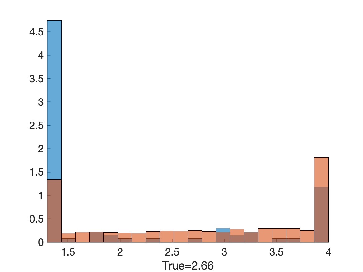
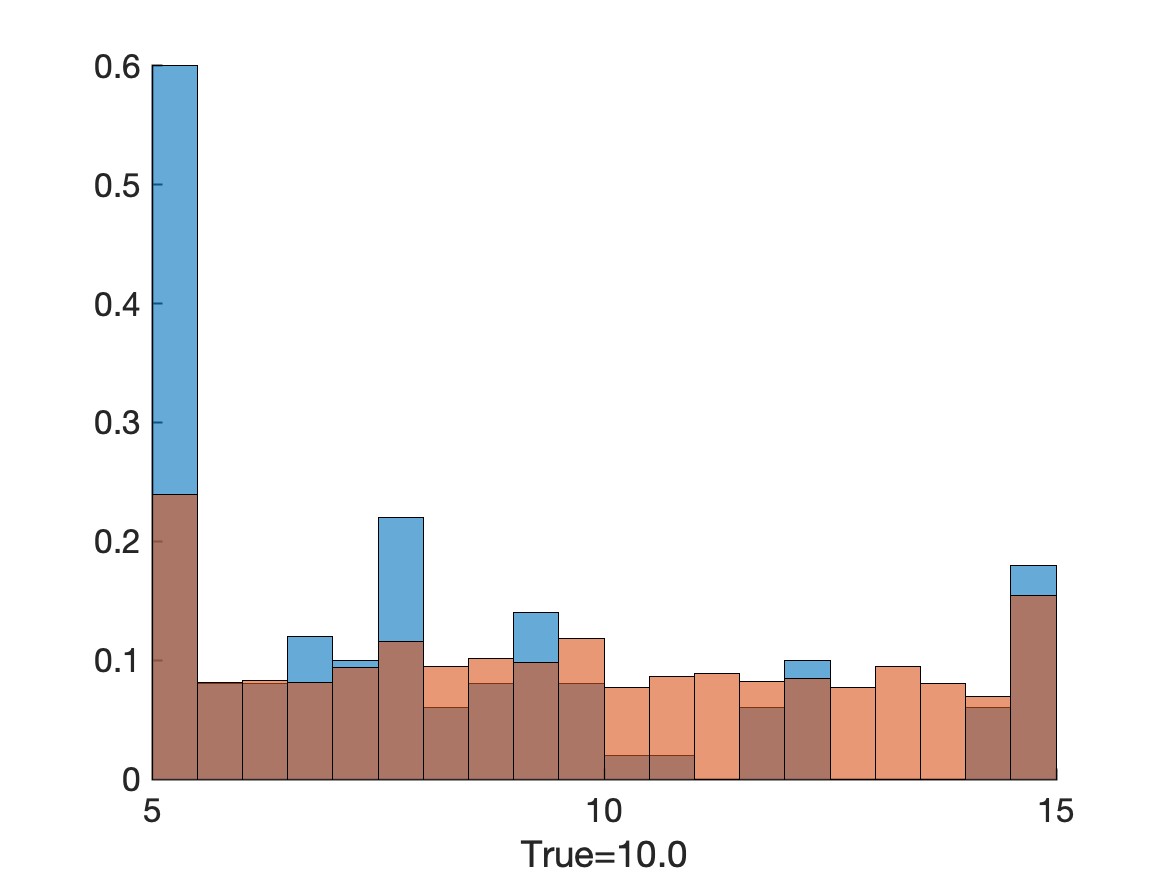
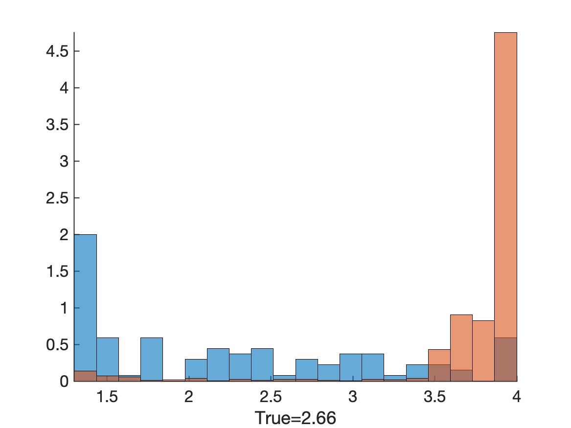
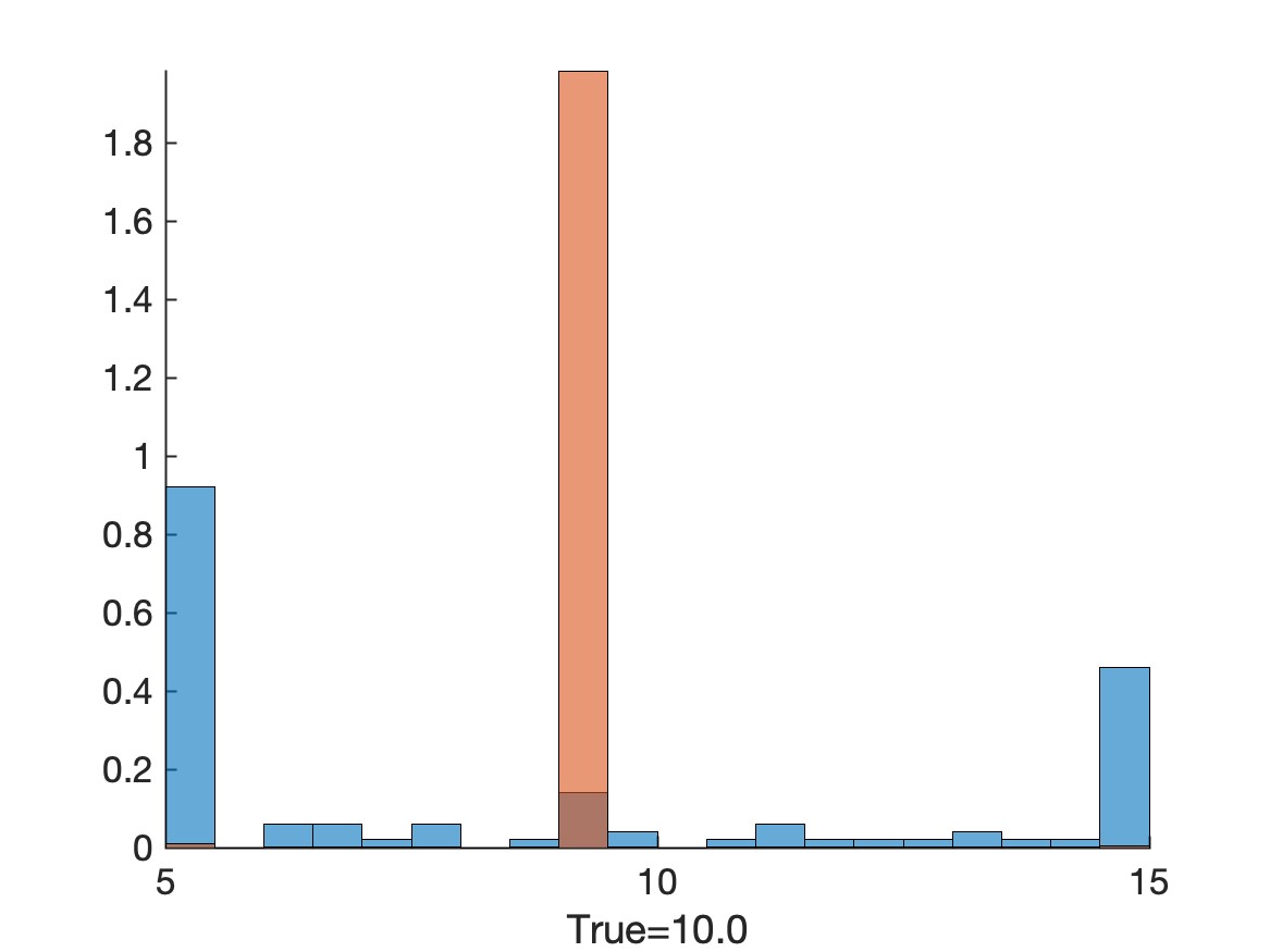
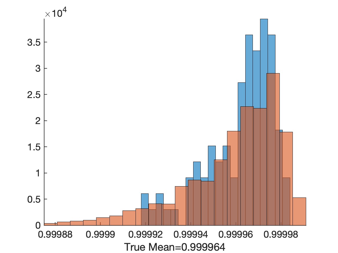
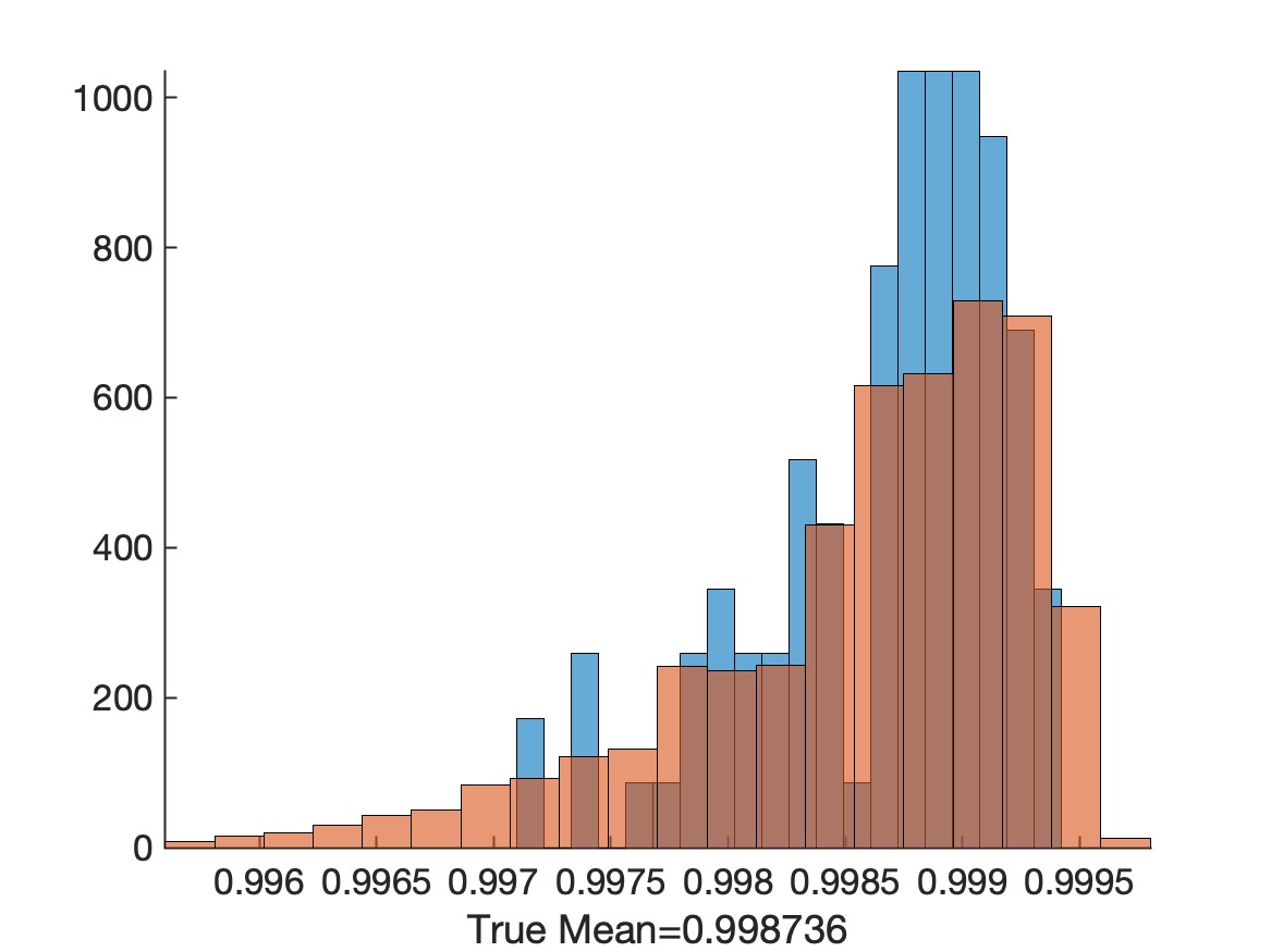
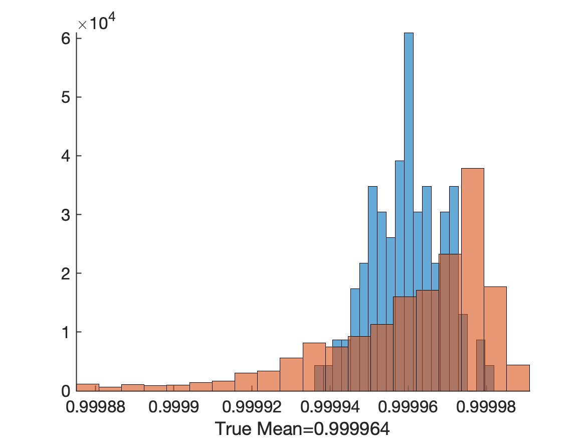
In the first example, the set of observed data is obtained as solution to (5.1) at time $T$ using randomly perturbed parameters, i.e., $\nu=\{z_{i}:i=1,\dots,K_{\max}\},$ and

$\displaystyle z_{i}=v(T,x^{*}+\xi_{i}),i=1,\dots,K_{\max}.$ (5.2)

Here, $\xi_{i}$ are the realization of a uniformly distributed random variable

$\displaystyle\xi\sim\otimes_{j=1}^{3}\mathcal{U}(-a^{j},a^{j}).$ (5.3)

We consider the Metropolis Monte Carlo method without information of the moments $\kappa.$ In the simulations, we compare using a Gaussian distribution or a gradient based approach to provide the proposal point $x_{p}.$ The further details of the implementation are stated in Section 7.2. In Figure 1 and Figure 2 we compare the two strategies for generating proposals. While the true mean is not exactly recovered, we observe that both strategies succeed in solving the minimization problem (1.1). The histograms show a concentration close to the true mean. The later is obtained as $v(T,x^{*})$ where $x^{*}$ is the true set of parameters without perturbation.

Refer to caption
Refer to caption
Refer to caption
Refer to caption
Figure 1: Fixed terminal time simulated by Metropolis Monte–Carlo using Gaussian proposals. The initial distribution $P_{0}$ is depicted in blue as a histogram. The histogram of the terminal distribution $P_{N}$ is shown in red. In the top part we show the histogram of the parameters, in the bottom part the corresponding histogram of the model evaluations, i.e. $\mu$. With the parameters and model evaluations similar, we show $x_{2}$ and $x_{3}$ and $v_{2}$ and $v_{3}$ in the lower part of the diagram, respectively. The value ’true mean’ represents the solution $v(T,x^{*})$ for the optimal parameter $x^{*}.$
Refer to caption
Refer to caption
Refer to caption
Refer to caption
Figure 2: Fixed terminal time simulated using gradient–based proposal updates. The initial distribution $P_{0}$ is depicted in blue as a histogram. The histogram of the terminal distribution $P_{N}$ is shown in red. In the top part we show the histogram of the parameters, in the bottom part the corresponding histogram of the model evaluations, i.e. $\mu$. With the parameters and model evaluations similar, we show $x_{2}$ and $x_{3}$ and $v_{2}$ and $v_{3}$ in the lower part of the diagram, respectively. The value ’true mean’ represents the solution $v(T,x^{*})$ for the optimal parameter $x^{*}.$

5.2 Running terminal time

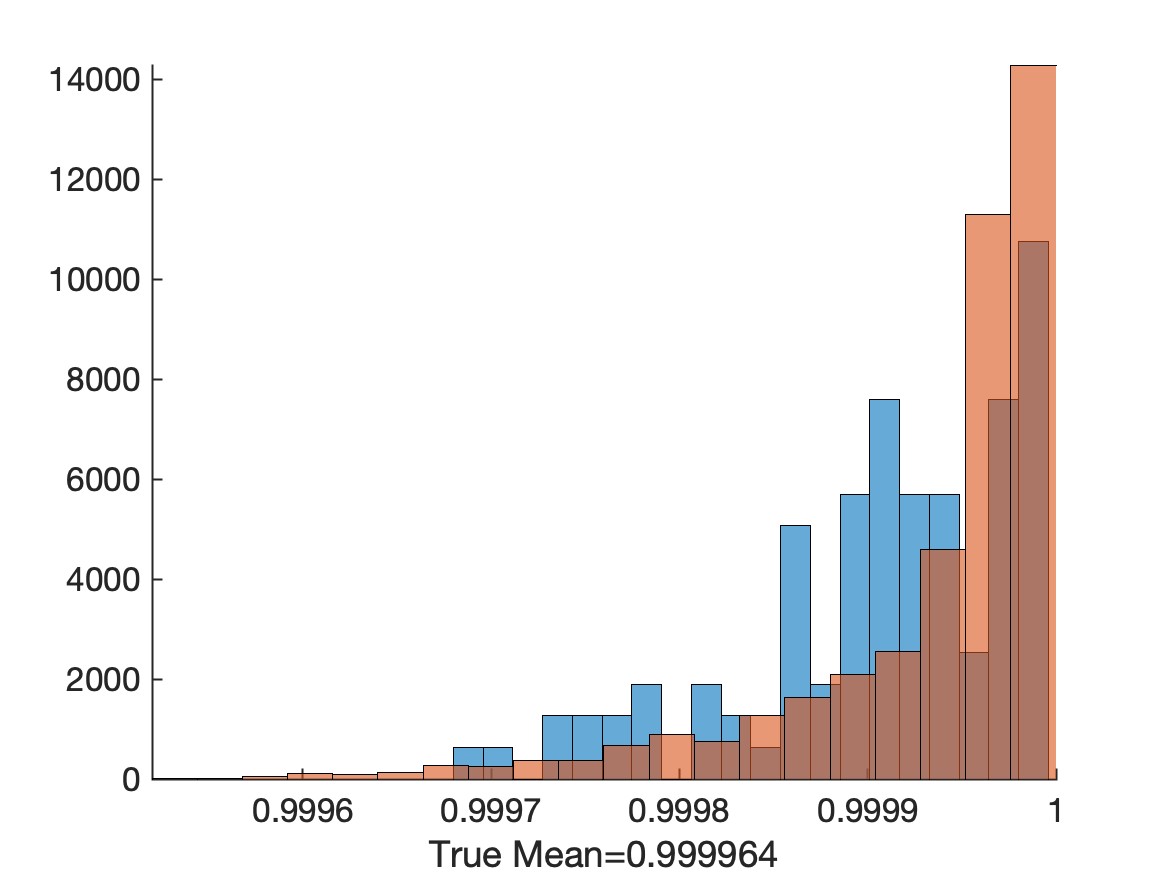
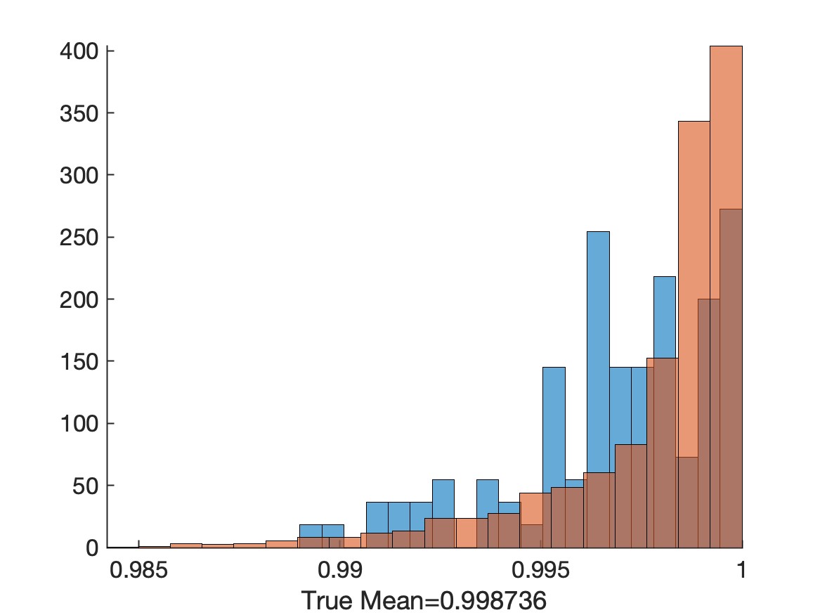
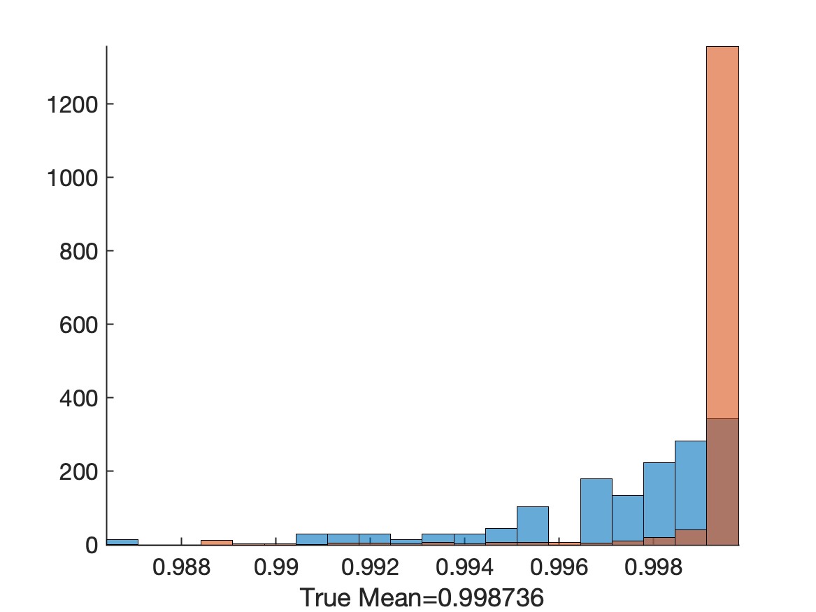
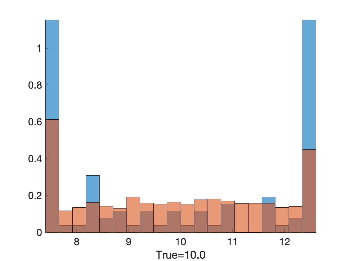
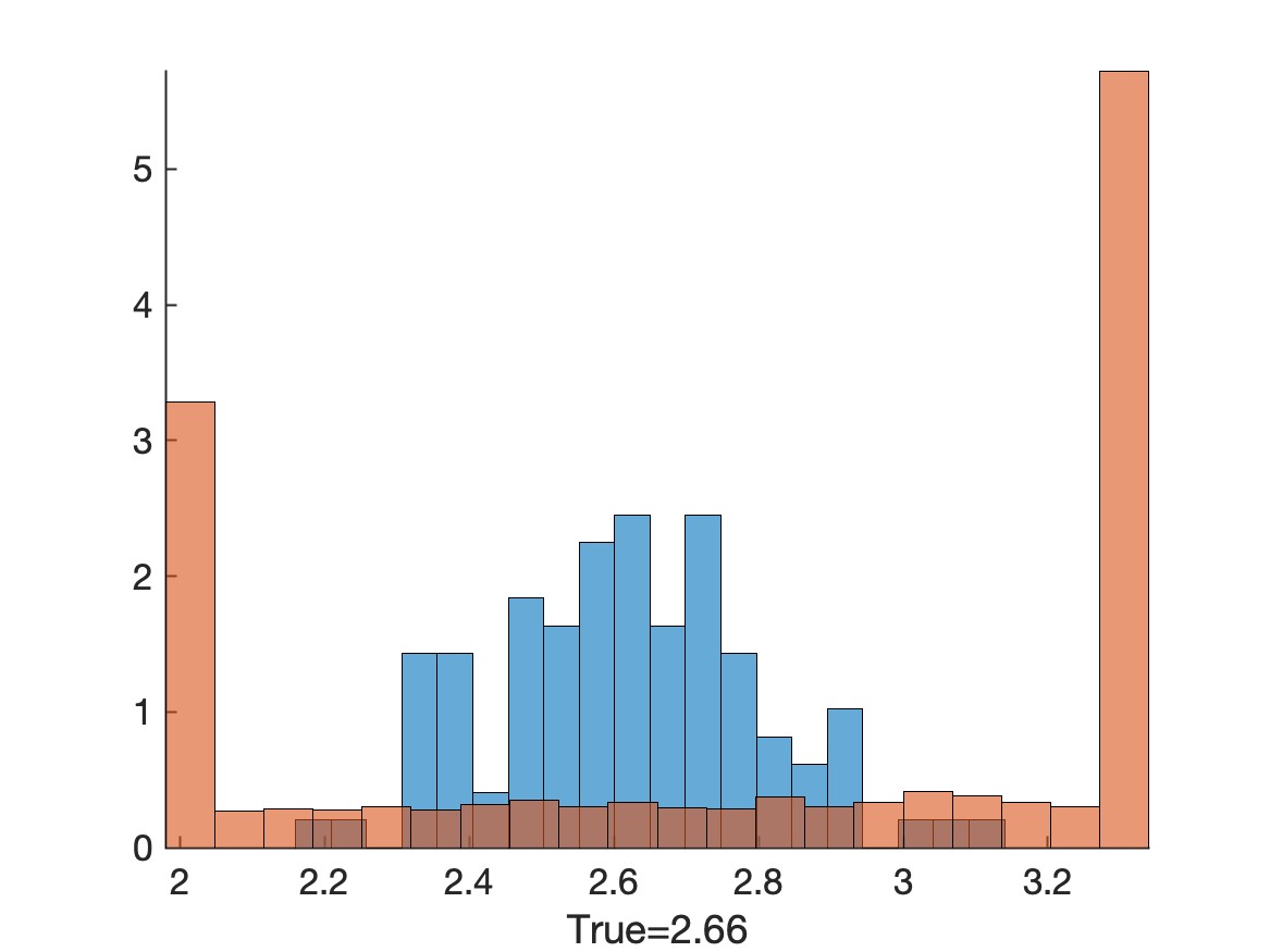
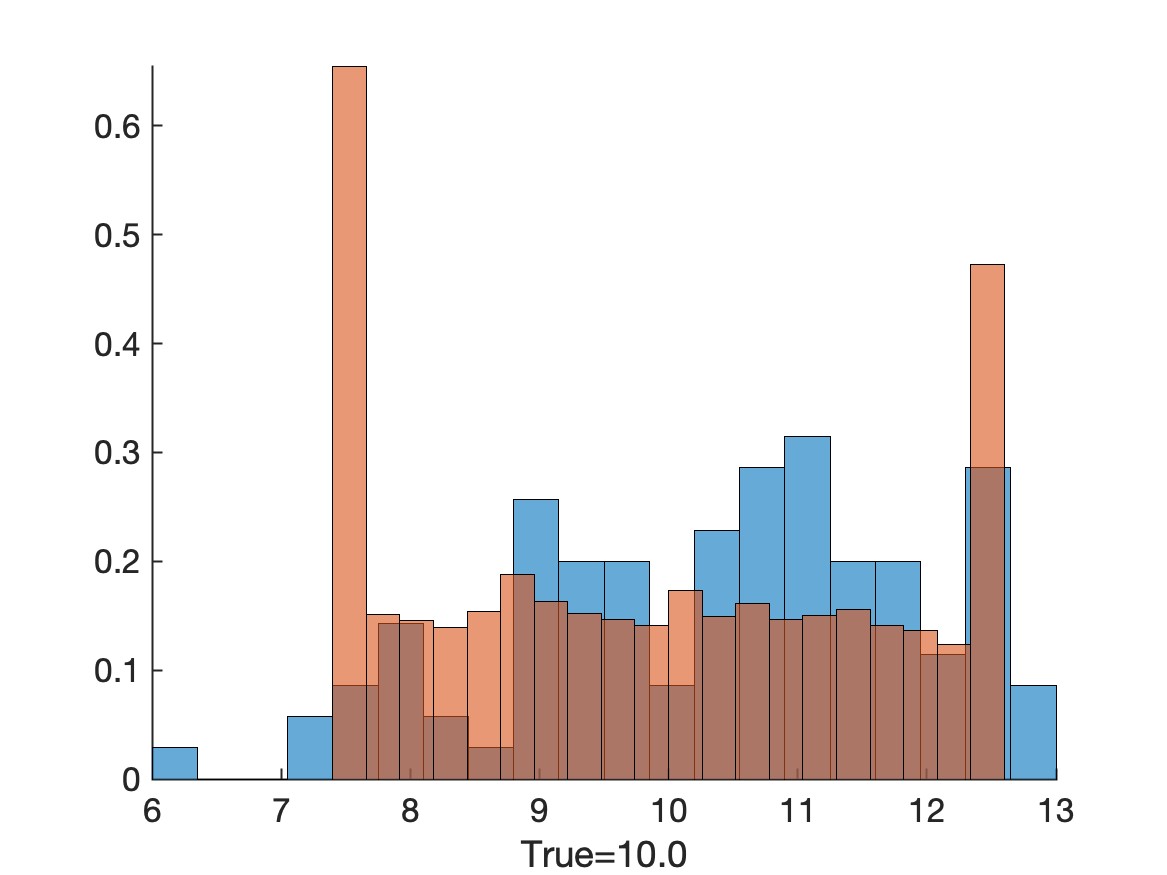
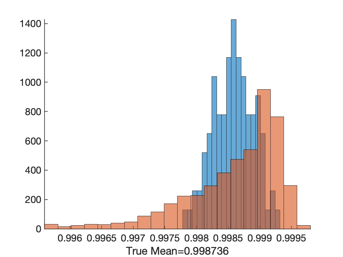
In the second example, we consider a problem where the time horizon is not fixed. Denote by $t_{i}=i\Delta t$ for $i=1,\dots,K_{\max}$ and with $K_{\max}\Delta t=T$ for a fixed terminal time $T.$ The set of data points $\nu=\{z_{i}:i=1,\dots,K_{\max}\}$ is given by the solution at time $t_{i}$ for perturbed parameters:

$\displaystyle z_{i}=v(t_{i},x^{*}+\xi_{i})$ (5.4)

where $\xi_{i}$ are realizations of a random variable $\xi$ distributed as in equation (5.3). We compare the Metropolis Monte Carlo method without and with using moment information on the identification problem (1.1). The proposal $x_{p}$ is obtained using a micro-macro decomposition using an indicator $\zeta$ as outlined in Section 4. The further details of the implementation are stated in Section 7.2. The results are depicted in Figure 3 and Figure 4, respectively. We observe that the micro–macro decomposition is feasible and leads to similar histograms compared with the Metropolis Monte Carlo method. The rate of the macroscopic updates is about $1\%$ in the reported results.

Refer to caption
Refer to caption
Refer to caption
Refer to caption
Figure 3: Running terminal time simulated using Metropolis Monte Carlo method. The initial distribution $P_{0}$ is depicted in blue as a histogram. The histogram of the terminal distribution $P_{N}$ is shown in red. In the top part we show the histogram of the parameters, in the bottom part the corresponding histogram of the model evaluations, i.e. $\mu$. With the parameters and model evaluations similar, we show $x_{2}$ and $x_{3}$ and $v_{2}$ and $v_{3}$ in the lower part of the diagram, respectively. The value ’true mean’ represents the solution $v(T,x^{*})$ for the optimal parameter $x^{*}.$
Refer to caption
Refer to caption
Refer to caption
Refer to caption
Figure 4: Running terminal time simulated using micro–macro decomposition. The initial distribution $P_{0}$ is depicted in blue as a histogram. The histogram of the terminal distribution $P_{N}$ is shown in red. In the top part we show the histogram of the parameters, in the bottom part the corresponding histogram of the model evaluations, i.e. $\mu$. With the parameters and model evaluations similar, we show $x_{2}$ and $x_{3}$ and $v_{2}$ and $v_{3}$ in the lower part of the diagram, respectively. The value ’true mean’ represents the solution $v(T,x^{*})$ for the optimal parameter $x^{*}.$

6 Summary

In this paper we developed a kinetic convergence theory for Metropolis Monte Carlo algorithms. The application to Bayesian type inverse problems, where the result is not one optimal parameter but a probability distribution in parameter space which optimally fits the given data, is considered. The kinetic theory allows for the theoretical reduction to lower dimensional problems which, in turn, allows for the efficient use of improved predictors an proposal distributions. All this leads to iterative Bayesian estimation procedures with a significant increase in the quality of the posterior distribution as well as an increase in computational efficiency.

Acknowledgments The authors thank the Deutsche Forschungsgemeinschaft (DFG, German Research Foundation) for the financial support through 320021702/GRK2326, 333849990/IRTG-2379, B04, B05 and B06 of 442047500/SFB1481, HE5386/19-3,22-1,23-1,25-1,26-1,27-1 and support from the European Unions Horizon Europe research and innovation programme under the Marie Sklodowska-Curie Doctoral Network Datahyking (Grant No. 101072546).

References

  • [1] M Bauer and F Cornu. Local detailed balance: a microscopic derivation. Journal of Physics A: Mathematical and Theoretical, 48(1):015008, dec 2014.
  • [2] S. Brooks, A. Gelman, G. Jones, and X. Meng. Handbook of Markov Chain Monte Carlo. CRC press, 2011.
  • [3] Tan Bui-Thanh, Omar Ghattas, James Martin, and Georg Stadler. A computational framework for infinite-dimensional Bayesian inverse problems Part I: The linearized case, with application to global seismic inversion. SIAM J. Sci. Comput., 35(6):A2494–A2523, 2013.
  • [4] D. Calvetti and E. Somersalo. Introduction to Bayesian Scientific Computing. Springer, 2007.
  • [5] Rafael Cano, Carmen Sordo, and José Gutiérrez. Applications of bayesian networks in meteorology. Wiley Interdisciplinary Reviews: Computational Statistics, 2004.
  • [6] Hudong Chen. $H$-theorem and generalized semi-detailed balance condition for lattice gas systems. J. Statist. Phys., 81(1-2):347–359, 1995.
  • [7] Albert Einstein. Investigations on the theory of the Brownian movement. Dover Publications, Inc., New York, 1956. Edited with notes by R. Fürth, Translated by A. D. Cowper.
  • [8] Heinz W. Engl, Karl Kunisch, and Andreas Neubauer. Convergence rates for Tikhonov regularisation of nonlinear ill-posed problems. Inverse Problems, 5(4):523–540, 1989.
  • [9] Dani Gamerman and Hedibert Freitas Lopes. Markov chain Monte Carlo. Texts in Statistical Science Series. Chapman & Hall/CRC, Boca Raton, FL, second edition, 2006. Stochastic simulation for Bayesian inference.
  • [10] Charles J. Geyer. Introduction to Markov chain Monte Carlo. In Handbook of Markov chain Monte Carlo, Chapman & Hall/CRC Handb. Mod. Stat. Methods, pages 3–48. CRC Press, Boca Raton, FL, 2011.
  • [11] M. Hairer, A. Stuart, and J. Voss. Signal processing problems on function space: Bayesian formulation, stochastic PDEs and effective MCMC methods. In The Oxford handbook of nonlinear filtering, pages 833–873. Oxford Univ. Press, Oxford, 2011.
  • [12] Bastian Harrach, Tim Jahn, and Roland Potthast. Regularizing linear inverse problems under unknown non-Gaussian white noise allowing repeated measurements. IMA J. Numer. Anal., 43(1):443–500, 2023.
  • [13] W. K. Hastings. Monte Carlo sampling methods using Markov chains and their applications. Biometrika, 57(1):97–109, 1970.
  • [14] P. Héas, F. Cérou, and M. Rousset. Chilled sampling for uncertainty quantification: a motivation from a meteorological inverse problem. Inverse Problems, 40(2):Paper No. 025004, 38, 2024.
  • [15] J. Kaipio and E. Somersalo. Statistical and Computational Inverse Problems. 0066-5452. Springer-Verlag New York, 2005.
  • [16] Kody Law, Andrew Stuart, and Konstantinos Zygalakis. Data assimilation, volume 62 of Texts in Applied Mathematics. Springer, Cham, 2015. A mathematical introduction.
  • [17] Aaron Myers, Alexandre H. Thiéry, Kainan Wang, and Tan Bui-Thanh. Sequential ensemble transform for Bayesian inverse problems. J. Comput. Phys., 427:Paper No. 110055, 21, 2021.
  • [18] Richard Nickl. Bayesian non-linear statistical inverse problems. Zurich Lectures in Advanced Mathematics. EMS Press, Berlin, [2023] ©2023.
  • [19] Daniel Sanz-Alonso, Andrew Stuart, and Armeen Taeb. Inverse problems and data assimilation, volume 107 of London Mathematical Society Student Texts. Cambridge University Press, Cambridge, 2023.
  • [20] Lutz Schimansky-Geier and Thorsten Pöschel, editors. Stochastic dynamics, volume 484 of Lecture Notes in Physics. Springer-Verlag, Berlin, 1997.
  • [21] A. M. Stuart. Inverse problems: a Bayesian perspective. Acta Numer., 19:451–559, 2010.
  • [22] T. Sullivan. Introduction to Uncertainty Quantification. Springer, 2015.
  • [23] Leila Taghizadeh, Ahmad Karimi, Benjamin Stadlbauer, Wolfgang J. Weninger, Eugenijus Kaniusas, and Clemens Heitzinger. Bayesian inversion for electrical-impedance tomography in medical imaging using the nonlinear poisson boltzmann equation. Computer Methods in Applied Mechanics and Engineering, 365:112959, 2020.
  • [24] Leila Taghizadeh, Amirreza Khodadadian, and Clemens Heitzinger. The optimal multilevel monte-carlo approximation of the stochastic drift diffusion poisson system. Computer Methods in Applied Mechanics and Engineering, 318:739–761, 2017.

7 Appendix

7.1 Technical proofs

Proof of Proposition 3.9:
Separating the terms in (3.4)into those containing the acceptance rate and the term independent of $\alpha$ gives, using the fact that $\int\tau(x|y,r)\ dx=1$ holds,

$\displaystyle\int\phi(x,\kappa)f(x,\kappa,s+h)\ dx\kappa=\int\phi(y,r+h\omega_{1}(y,r,s))f(y,r,s)\ dyr+$ (7.1)
$\displaystyle h\int[\phi(x,r+h\omega_{1}(x,r,s))-\phi(y,r+h\omega_{1}(y,r,s))]\times$ (7.2)
$\displaystyle\alpha(x,r+h\omega_{1}(x,r,s),y,r+h\omega_{1}(y,r,s))\tau(x|y,r)f(y,r,s)\ dxyr$ (7.3)

The first integral on the right hand side of (7.1) gives after Taylor expansion in the stepsize $h$

$\displaystyle\int\phi(y,r+h\omega_{1}(y,r,s))f(y,r,s)\ dyr=$ (7.4)
$\displaystyle\int\phi(y,r)f(y,r,s)\ dyr+\int h\nabla_{2}\phi(y,r)\cdot\omega_{1}(y,r,s)f(y,r,s)\ dyr+o(h)\ .$ (7.5)

The second term on the right hand side of (7.1) gives, up to order $o(h)$

$\displaystyle h\int[\phi(x,r+h\omega_{1}(x,r,s))-\phi(y,r+h\omega_{1}(y,r,s))]\times$ (7.6)
$\displaystyle\alpha(x,r+h\omega_{1}(x,r,s),y,r+h\omega_{1}(y,r,s))\tau(x|y,r)f(y,r,s)\ dxyr=$ (7.7)
$\displaystyle h\int[\phi(x,r)-\phi(y,r)]K(x,y,r)f(y,r,s)\ dxyr+o(h)\ ,$ (7.8)

with the kernel $K$ given by (3.9). Combining (7.4) and (7.6), letting $h\rightarrow 0,\ N\rightarrow\infty$ gives

$\displaystyle\int\phi(x,\kappa)\partial_{s}f(x,\kappa,s)\ dx\kappa=$ (7.9)
$\displaystyle\int\nabla_{2}\phi(y,r)\cdot\omega_{1}(y,r,s)f(y,r,s)\ dyr+\int[\phi(x,r)-\phi(y,r)]K(x,y,r)f(y,r,s)\ dxyr$ (7.10)

which is the weak form of

$\displaystyle\partial_{s}f(x,\kappa,s)=$ (7.11)
$\displaystyle-div_{\kappa}[\omega_{1}(x,\kappa,s)f]+\int K(x,y,\kappa)f(y,\kappa,s)\ dy-\int K(y,x,\kappa)f(x,\kappa,s)\ dy$ (7.12)

with the kernel $K$ given by (3.9).  

Proof of Proposition 3.2 :
We define the symmetrized kernel $K_{sym}$ by $K_{sym}(x,y)=K(x,y)f_{\infty}(y)=\alpha(x,y)\tau(x|y)f_{\infty}(y)$ satisfying, according to the detail balance condition (3.11), the symmetry $K_{sym}(x,y)=K_{sym}(y,x)$. This makes (3.10) into

$$\int\phi(x)\partial_{s}f(x,s)\ dx=\int[\phi(x)-\phi(y)]K_{sym}(x,y)\frac{f(y,s)}{f_{\infty}(y)}\ dxy\ \forall\phi\ .$$

Interchanging the integration variables $x\leftrightarrow y$ in the integral on the right hand side gives (because of the symmetry of $K_{sym}$)

$$\int\phi(x)\partial_{s}f(x,s)\ dx=\int[\phi(y)-\phi(x)]K_{sym}(x,y)\frac{f(x,s)}{f_{\infty}(x)}\ dxy\ .\ \forall\phi\ ,$$

Summing these two equations gives

$$2\int\phi(x)\partial_{s}f(x,s)\ dx=\int[\phi(x)-\phi(y)]K_{sym}(x,y)[\frac{f(y,s)}{f_{\infty}(y)}-\frac{f(x,s)}{f_{\infty}(x)}\ \ dxy\ .\ \forall\phi\ .$$ (7.13)

First, we see from (7.13) that we obtain a steady state for $f(x,s)=f_{\infty}(x)$ since the right hand side vanishes for all test functions $\phi$. Second, choosing the special test function $\phi=\frac{f(x,s)}{f_{\infty}(x)}$

$$2\int\frac{f(x,s)}{f_{\infty}(x)}\partial_{s}f(x,s)\ dx=\partial_{s}\int\frac{f(x,s)^{2}}{f_{\infty}(x)}\ dx=-\int K_{sym}(x,y)[\frac{f(y,s)}{f_{\infty}(y)}-\frac{f(x,s)}{f_{\infty}(x)}]^{2}\ \ dxy\leq 0\ .$$

Thus, the convex entropy functional $H_{f}(s)=\int\frac{f(x,s)^{2}}{f_{\infty}(x)}\ dx$ decays monotonically until the limit $f=f_{\infty}$ is reached.  

Proof of Proposition 3.3
We separate (3.19) into a term which reduces to the pure Browninan motion (for $\beta=0$) and a term dependent on the rejection rate $\beta$.

$\displaystyle\int\phi(x,\kappa)f(x,\kappa,s+h)\ dx\kappa=A+B$ (7.14)
$\displaystyle A=\int\phi(x,\omega(x,r,s))\frac{1}{(\sqrt{h}\sigma(y,r))^{d}}\psi(\frac{x-y-hE(y,r)}{\sqrt{h}\sigma(y,r)})f(y,r,s)\ dyrx$ (7.15)
$\displaystyle B=\int[\phi(y,\omega(y,r,s))-\phi(x,\omega(x,r,s))]\beta(x,\omega(x,r,s),y,\omega(y,r,s))\times$ (7.16)
$\displaystyle\frac{1}{(\sqrt{h}\sigma(y,r))^{d}}\psi(\frac{x-y-hE(y,r)}{\sqrt{h}\sigma(y,r)})f(y,r,s)\ dyrx\ .$ (7.17)

This gives for the term $A$ in (7.15), after the variable transformation $x\rightarrow y+hE+\sqrt{h}\sigma x,\ dx\rightarrow\sigma^{d}dx$,

$$A=\int\phi(y+hE(y,r)+\sqrt{h}\sigma(y,r)x,\omega(y+hE+\sqrt{h}\sigma x,r,s))\psi(x)f(y,r,s)\ dyrx$$ (7.18)

The term $A$ should (for $\beta=0$) give the classical Brownian motion term. Similarly, for the term $B$ in (7.16) (the correction if we do not always accept) we obtain, normalizing $\tau$ and transforming in the integral

$$B=[\phi(y,\omega(y,r,s))-\phi(y+hE+\sqrt{h}\sigma x,\omega(y+hE+\sqrt{h}\sigma x,r,s))]\times$$ (7.19)
$$\beta(y+hE+\sqrt{h}\sigma x,\omega(y+hE+\sqrt{h}\sigma x,r,s),y,\omega(y,r,s))\psi(x)f(y,r,s)\ dyrx,$$

We will still have to move the zero order term in $A$ to the left hand side and divide by the stepsize $h$ to obtain a derivative in $s$. So, what remains is to expand (7.18) and (7.19) for small stepsizes $h$ up to $o(h)$.

Expansion of $A$. We have from (7.18)

$$A=\int\phi(y+hE(y,r)+\sqrt{h}\sigma(y,r)x,\omega(y+hE+\sqrt{h}\sigma x,r,s))\psi(x)f(y,r,s)\ dyrx$$

We first expand $\phi$ in terms of the perturbation in the first variable $y$.

$\displaystyle A=A_{0}+A_{1}+A_{2}+o(h)\ .$ (7.20)
$\displaystyle A_{0}=\int\phi(y,\omega(y+hE+\sqrt{h}\sigma x,r,s))\psi(x)f(y,r,s)\ dyrx\ .$ (7.21)
$\displaystyle A_{1}=\int(hE(y,r)+\sqrt{h}\sigma(y,r)x)\partial_{1}\phi(y,\omega(y+hE+\sqrt{h}\sigma x,r,s))\psi(x)f(y,r,s)\ dyrx$ (7.22)
$\displaystyle A_{2}=\int\frac{1}{2}(hE(y,r)+\sqrt{h}\sigma(y,r)x)^{2}\partial_{1}^{2}\phi(y,\omega(y+hE+\sqrt{h}\sigma x,r,s))\psi(x)f(y,r,s)\ dyrx$ (7.23)

First we write the proposed moments $\omega(x,\kappa,s)$ in (3.16) as a $O(h)$ perturbation around the current moments $\kappa$:

$$\omega(x,\kappa,s)=\kappa+h\omega_{1}(x,\kappa,s),\ \omega_{1}(x,\kappa,s)=\frac{\Delta\kappa(x)-\kappa}{s+h}\ .$$ (7.24)

expanding the growth $\omega$ in the moments using $\omega(y,r,s)=r+h\omega_{1}(y,r,s)$

$\displaystyle A_{0}=\int\phi(y,r+h\omega_{1}(y+hE+\sqrt{h}\sigma x,r,s))\psi(x)f(y,r,s)\ dyrx$ (7.25)
$\displaystyle=\int\phi(y,r)\psi(x)f(y,r,s)\ dyrx+\int(h\omega_{1}(y+hE+\sqrt{h}\sigma x,r,s)\cdot\nabla_{r}\phi(y,r))\psi(x)f(y,r,s)\ dyrx+O(h^{2})$ (7.26)
$\displaystyle=\int\phi(y,r)\psi(x)f(y,r,s)\ dyrx+\int h\omega_{1}(y,r,s)\cdot\nabla_{r}\phi(y,r)\psi(x)f(y,r,s)\ dyrx+o(h)$ (7.27)

integrating against the normalized distribution $\psi$ gives

$$A_{0}=\int\phi(y,r)f(y,r,s)\ dyr+\int h\omega_{1}(y,r,s)\cdot\nabla_{r}\phi(y,r)f(y,r,s)\ dyr+o(h)\ .$$

We proceed in the same way with the terms $A_{1}$ and $A_{2}$:

$\displaystyle A_{1}=\int(hE(y,r)+\sqrt{h}\sigma(y,r)x)\cdot\nabla_{y}\phi(y,r+h\omega_{1}(y+hE+\sqrt{h}\sigma x,r,s))\psi(x)f(y,r,s)\ dyrx$ (7.28)
$\displaystyle=\int(hE(y,r)+\sqrt{h}\sigma(y,r)x)\cdot\nabla_{y}\phi(y,r))\psi(x)f(y,r,s)\ dyrx+O(h^{3/2})$ (7.29)
$\displaystyle=\int hE(y,r)\cdot\nabla_{y}\phi(y,r)f(y,r,s)\ dyr+O(h^{3/2})\ .$ (7.30)

For $A_{2}$ we obtain

$\displaystyle A_{2}=\int\frac{1}{2}(hE(y,r)+\sqrt{h}\sigma(y,r)x)^{2}\partial_{1}^{2}\phi(y,r+h\omega_{1}(y+hE+\sqrt{h}\sigma x,r,s))\psi(x)f(y,r,s)\ dyrx$ (7.31)
$\displaystyle=\int\frac{1}{2}(hE(y,r)+\sqrt{h}\sigma(y,r)x)^{2}\partial_{1}^{2}\phi(y,r)\psi(x)f(y,r,s)\ dyrx+O(h^{2})$ (7.32)
$\displaystyle=\frac{1}{2}h\int\sigma(y,r)^{2}(x)^{2}\partial_{1}^{2}\phi(y,r)\psi(x)f(y,r,s)\ dyrx+O(h^{3/2})$ (7.33)
$\displaystyle=\frac{1}{2}h\int\sigma(y,r)^{2}x_{j}x_{k}\partial_{y_{j}y_{k}}\phi(y,r)\psi(x)f(y,r,s)\ dyrx+O(h^{3/2})$ (7.34)
$\displaystyle=\frac{1}{2}h\int\sigma(y,r)^{2}f(y,r,s)div_{y}\nabla_{y}\phi(y,r)\ dyr+O(h^{3/2})$ (7.35)

so, we have for the pure Brownian motion term (with a zero rejection rate $\beta=0$) $A=A_{0}+A_{1}+A_{2}+o(h)$ with

$\displaystyle A=\int\phi(y,r)f(y,r,s)\ dyr+\int h\omega_{1}(y,r,s)\cdot\nabla_{r}\phi(y,r)f(y,r,s)\ dyr$ (7.36)
$\displaystyle+\int hE(y,r)\cdot\nabla_{y}\phi(y,r)f(y,r,s)\ dyr+\frac{1}{2}h\int\sigma(y,r)^{2}f(y,r,s)div_{y}\nabla_{y}\phi(y,r)\ dyr+o(h)\ .$ (7.37)

Expansion of $B$: We define the difference in the argument of the test function in (7.19) as

$$\Delta\phi(x,y,r,s)=[\phi(y,\omega(y,r,s))-\phi(y+hE+\sqrt{h}\sigma x,\omega(y+hE+\sqrt{h}\sigma x,r,s))]$$

with $E=E(y,r)$ and $\sigma=\sigma(y,r)$ and, from (7.19) we write

$$B=\int\Delta\phi(x,y,r,s)\beta(y+hE+\sqrt{h}\sigma x,\omega(y+hE+\sqrt{h}\sigma x,r,s),y,\omega(y,r,s))\psi(x)f(y,r,s)\ dyrx\ .$$

Again, we use $\omega(y,r,s)=r+h\omega_{1}(y,r,s)$. Expanding the shift in $y$ in $\Delta\phi$ gives

$\displaystyle\Delta\phi(x,y,r,s)=[\phi(y,\omega(y,r,s))-\phi(y+hE+\sqrt{h}\sigma x,\omega(y+hE+\sqrt{h}\sigma x,r,s))]$ (7.38)
$\displaystyle=T_{0}+T_{1}+T_{2}+O(h^{3/2})\mbox{ for }$ (7.39)
$\displaystyle T_{0}=\phi(y,\omega(y,r,s))-\phi(y,\omega(y+hE+\sqrt{h}\sigma x,r,s))$ (7.40)
$\displaystyle T_{1}=-(hE+\sqrt{h}\sigma x)\cdot\nabla_{1}\phi(y,\omega(y+hE+\sqrt{h}\sigma x,r,s))$ (7.41)
$\displaystyle T_{2}=\frac{1}{2}(hE+\sqrt{h}\sigma x)^{2}\cdot\partial_{1}^{2}\phi(y,\omega(y+hE+\sqrt{h}\sigma x,r,s))$ (7.42)

Again, expanding $\omega$ using $\omega(y,r,s)=r+h\omega_{1}(y,r,s)$ gives for $T_{0},T_{1},T_{2}$

$\displaystyle T_{0}$ $\displaystyle=\phi(y,r+h\omega_{1}(y,r,s))-\phi(y,r+h\omega_{1}(y+hE+\sqrt{h}\sigma x,r,s))$ (7.43)
$\displaystyle=\phi(y,r)-\phi(y,r)$ (7.44)
$\displaystyle=+h\omega_{1}(y,r,s)\partial_{2}\phi(y,r)-h\omega_{1}(y+hE+\sqrt{h}\sigma x)\partial_{2}\phi(y,r)=O(h^{3/2})\ ,$ (7.45)

and for $T_{1}$ and $T_{2},$ respectively:

$\displaystyle T_{1}$ $\displaystyle=-(hE+\sqrt{h}\sigma x)\cdot\nabla_{1}\phi(y,r+h\omega_{1}(y+hE+\sqrt{h}\sigma x,r,s))=-(hE+\sqrt{h}\sigma x)\partial_{1}\phi(y,r)+O(h^{3/2})\ ,$ (7.46)
$\displaystyle T_{2}$ $\displaystyle=\frac{1}{2}(hE+\sqrt{h}\sigma x)^{2}\cdot\partial_{1}^{2}\phi(y,r+h\omega_{1}(y+hE+\sqrt{h}\sigma x,r,s))=\frac{1}{2}(hE+\sqrt{h}\sigma x)^{2}\cdot\partial_{1}^{2}\phi(y,r)+O(h^{2})\ .$ (7.47)

So, altogether, we have

$$\Delta\phi(x,y,r,s)=-(hE+\sqrt{h}\sigma x)\cdot\nabla_{1}\phi(y,r)+\frac{1}{2}(hE+\sqrt{h}\sigma x)^{2}\cdot\partial_{1}^{2}\phi(y,r)+O(h^{3/2})$$

or

$$\Delta\phi(x,y,r,s)=-(hE+\sqrt{h}\sigma x)\cdot\nabla_{1}\phi(y,r)+\frac{1}{2}h\sigma^{2}x^{2}\cdot\partial_{1}^{2}\phi(y,r)+O(h^{3/2})$$ (7.48)

Expansion of $\beta$. We note, that $\Delta\phi=O(\sqrt{h})$. So, we have to expand $\beta$ only up to $o(\sqrt{h})$ to obtain an expression for the product $\Delta\phi\beta$ up to order $o(h)$. We first expand again in the state variable:

$\displaystyle\beta(y+hE+\sqrt{h}\sigma x,\omega(y+hE+\sqrt{h}\sigma x,r,s),y,\omega(y,r,s))=\beta_{0}+\beta_{1}+o(\sqrt{h}),$ (7.49)
$\displaystyle\beta_{0}=\beta(y,\omega(y+hE+\sqrt{h}\sigma x,r,s),y,\omega(y,r,s))$ (7.50)
$\displaystyle\beta_{1}=(hE+\sqrt{h}\sigma x)\partial_{1}\beta(y,\omega(y+hE+\sqrt{h}\sigma x,r,s),y,\omega(y,r,s))$ (7.51)

Expansion in the moment corrections $\omega$ gives, using $\omega(y,r,s)=r+h\omega_{1}(y,r,s)$

$\displaystyle\beta_{0}=\beta(y,r+h\omega_{1}(y+hE+\sqrt{h}\sigma x,r,s),y,r+h\omega_{1}(y,r,s))=\beta(y,r,y,r)+o(\sqrt{h})$ (7.52)
$\displaystyle\beta_{1}=(hE+\sqrt{h}\sigma x)\cdot\nabla_{1}\beta(y,r+h\omega_{1}(y+hE+\sqrt{h}\sigma x,r,s),y,r+h\omega_{1}(y,r,s))=$ (7.53)
$\displaystyle(hE+\sqrt{h}\sigma x)\cdot\nabla_{1}\beta(y,r,y,r)+o(\sqrt{h})$ (7.54)

Therefore, we have

$$\beta(y+hE+\sqrt{h}\sigma x,\omega(y+hE+\sqrt{h}\sigma x,r,s),y,\omega(y,r,s))=$$
$$\beta(y,r,y,r)+(hE+\sqrt{h}\sigma x)\partial_{1}\beta(y,r,y,r)+o(\sqrt{h})$$ (7.55)

multiplying $\Delta\phi$ with $\beta$ from (7.48) and (7.55) gives

$\displaystyle\Delta\phi\beta=[-(hE+\sqrt{h}\sigma x)\cdot\nabla_{1}\phi(y,r)+\frac{1}{2}h\sigma^{2}x^{2}\cdot\partial_{1}^{2}\phi(y,r)+O(h^{3/2})]\times$ (7.56)
$\displaystyle[\beta(y,r,y,r)+(hE+\sqrt{h}\sigma x)\cdot\nabla_{1}\beta(y,r,y,r)+o(\sqrt{h})]$ (7.57)
$\displaystyle\Delta\phi\beta=-(hE+\sqrt{h}\sigma x)\cdot\nabla_{1}\phi(y,r)\beta(y,r,y,r)+\frac{1}{2}h\sigma^{2}x^{2}\cdot\partial_{1}^{2}\phi(y,r)\beta(y,r,y,r)$ (7.58)
$\displaystyle-(hE+\sqrt{h}\sigma x)\cdot\nabla_{1}\phi(y,r)(hE+\sqrt{h}\sigma x)\partial_{1}\beta(y,r,y,r)$ (7.59)
$\displaystyle+\frac{1}{2}h\sigma^{2}x^{2}\partial_{1}^{2}\phi(y,r)(hE+\sqrt{h}\sigma x)\partial_{1}\beta(y,r,y,r)+o(h)$ (7.60)

neglecting the $o(h)$ terms gives

$\displaystyle\Delta\phi\beta=-(hE+\sqrt{h}\sigma x)\cdot\nabla_{1}\phi(y,r)\beta(y,r,y,r)+\frac{1}{2}h\sigma^{2}x^{2}\cdot\partial_{1}^{2}\phi(y,r)\beta(y,r,y,r)$ (7.61)
$\displaystyle-h[\sigma x\partial_{1}\phi(y,r)][\sigma x\partial_{1}\beta(y,r,y,r)]+o(h)$ (7.62)

integrating against the normalized distribution $\psi$, using $\int(1,x,xx^{T})\psi(x)\ dx=(1,0,\;Id)$ gives

$\displaystyle\int\Delta\phi\beta\psi(x)\ dx=-hE\cdot\nabla_{y}\phi(y,r)\beta(y,r,y,r)+\frac{1}{2}h\sigma^{2}\beta(y,r,y,r)div_{y}\nabla_{y}\phi(y,r)$ (7.63)
$\displaystyle-h\sigma^{2}\nabla_{y}\phi(y,r)\cdot\nabla_{1}\beta(y,r,y,r)+o(h)$ (7.64)

multiplying with $f(y,r)$ and integrating $dyr$ give the term $B$ in (7.19) up to terms of order $o(h)$.

$\displaystyle B$ $\displaystyle=\int[-hE\cdot\nabla_{y}\phi(y,r)\beta(y,r,y,r)+\frac{1}{2}h\sigma^{2}\beta(y,r,y,r)div_{y}\nabla_{y}\phi(y,r)$ (7.65)
$\displaystyle-h\sigma^{2}\nabla_{y}\phi(y,r)\cdot\nabla_{1}\beta(y,r,y,r)]f(y,r,s)\ dyr+o(h)$ (7.66)

combining (7.36) and (7.65) gives

$$\int\phi(x,\kappa)f(x,\kappa,s+h)\ dx\kappa=A+B+o(h)$$

or, after changing the variables $y\rightarrow x$ and $r\rightarrow\kappa$ in the integrals on the right hand side

$\displaystyle\int\phi(x,\kappa)f(x,\kappa,s+h)\ dx\kappa=$ (7.67)
$\displaystyle\int\phi(x,\kappa)f(x,\kappa,s)\ dx\kappa+\int h\omega_{1}(x,\kappa,s)\cdot\nabla_{\kappa}\phi(x,\kappa)f(x,\kappa,s)\ dx\kappa$ (7.68)
$\displaystyle+\int hE(x,\kappa)\cdot\nabla_{x}\phi(x,\kappa)f(x,\kappa,s)\ dx\kappa+\frac{1}{2}h\int\sigma(x,\kappa)^{2}f(x,\kappa,s)div_{x}\nabla_{x}\phi(x,\kappa)\ dx\kappa$ (7.69)
$\displaystyle+\int[-hE\cdot\nabla_{x}\phi(x,\kappa)\beta(x,\kappa,x,\kappa)+\frac{1}{2}h\sigma^{2}\beta(x,\kappa,x,\kappa)div_{x}\nabla_{x}\phi(x,\kappa)$ (7.70)
$\displaystyle-h\sigma^{2}\nabla_{x}\phi(x,\kappa)\cdot\nabla_{1}\beta(x,\kappa,x,\kappa)]f(x,\kappa,s)\ dx\kappa+o(h)$ (7.71)

moving the $O(1)$ term $\int\phi(x,\kappa)f(x,\kappa,s)\ dx\kappa$ to the left of the equality sign and dividing by the stepsize $h$, and letting $h\rightarrow 0$ gives for all test functions $\phi:$

$\displaystyle\int\phi(x,\kappa)\partial_{s}f(x,\kappa,s)\ dx\kappa=$ (7.72)
$\displaystyle\int\omega_{1}(x,\kappa,s)\cdot\nabla_{\kappa}\phi(x,\kappa)f(x,\kappa,s)\ dx\kappa$ (7.73)
$\displaystyle+\int E(x,\kappa)\cdot\nabla_{x}\phi(x,\kappa)f(x,\kappa,s)\ dx\kappa+\frac{1}{2}\int\sigma(x,\kappa)^{2}f(x,\kappa,s)div_{x}\nabla_{x}\phi(x,\kappa)\ dx\kappa$ (7.74)
$\displaystyle+\int[-E\cdot\nabla_{x}\phi(x,\kappa)\beta(x,\kappa,x,\kappa)+\frac{1}{2}\sigma^{2}\beta(x,\kappa,x,\kappa)div_{x}\nabla_{x}\phi(x,\kappa)$ (7.75)
$\displaystyle-\sigma^{2}\nabla_{x}\phi(x,\kappa)\cdot\nabla_{1}\beta(x,\kappa,x,\kappa)]f(x,\kappa,s)\ dx\kappa+o(1)$ (7.76)

After integrating by parts this is the weak form of

$\displaystyle\partial_{s}f(x,\kappa,s)=-div_{\kappa}[\omega_{1}(x,\kappa,s)f(x,\kappa,s)]$ (7.77)
$\displaystyle-div_{x}[E(x,\kappa)f(x,\kappa,s)]+\frac{1}{2}div_{x}\nabla_{x}[\sigma(x,\kappa)^{2}f(x,\kappa,s)]$ (7.78)
$\displaystyle+div_{x}[\sigma^{2}\nabla_{1}\beta(x,\kappa,x,\kappa)f(x,\kappa,s)]\ .$ (7.79)

We consolidate

$\displaystyle\partial_{s}f(x,\kappa,s)=-div_{\kappa}[\omega_{1}(x,\kappa,s)f(x,\kappa,s)]$ (7.80)
$\displaystyle+div_{x}[E(x,\kappa)(\beta(x,\kappa,x,\kappa)-1)f(x,\kappa,s)+\sigma^{2}\nabla_{1}\beta(x,\kappa,x,\kappa)f(x,\kappa,s)]$ (7.81)
$\displaystyle+\frac{1}{2}div_{x}\nabla_{x}[\sigma(x,\kappa)^{2}(1+\beta(x,\kappa,x,\kappa))f(x,\kappa,s)]$ (7.82)


7.2 Implementation details

We report on the details required for the simulation of the Metropolis Monte Carlo algorithm of Section 2.1. Here, all parameter choices are detailed. For readability we present a the parameters in the order of appearance.

The total number of time steps $n=1,\dots,N$ is $N=10^{\prime}000$ in all simulations.

In all cases we set $T=25$, $K_{\max}=10^{\prime}000$ and $a_{1}=a_{3}=10$ and $a_{2}=1.$

The moments $\kappa$ defined by equation (2.1) we consider $\kappa=(\kappa_{1},\sigma)$ defined by

$\displaystyle\kappa^{n}_{1}=\frac{1}{n}\sum_{j=1}^{n}x_{j},\;\sigma^{n}=\kappa^{n}_{2}-(\kappa_{1}^{n})^{2},\kappa_{2}^{n}=\frac{1}{n}\sum_{i=1}^{n}\left(x_{j}\right)^{2}.$ (7.83)

According to remark (2.3), the Monte Carlo algorithm requires a start up phase. We realize this by producing an initial distribution obtained by considering $i=1,\dots,N$ simulations of model (5.1) with parameter $x_{i}:=x^{*}+\xi_{i}$ and $\xi_{i}$ being a realization of the random variable $\xi$ distributed according to equation (5.3). This yields the distribution

$\displaystyle P_{0}(x)=\frac{1}{N_{0}}\sum_{i=1}^{N_{0}}\delta(x-x_{i}),$ (7.84)

and the corresponding moments $\kappa_{0}.$ In our simulations we set ${N_{0}}=100.$

The ODE system (5.1) is solved on the time interval $[0,T]$ using an explicit 3(2) Runge-Kutta of the Matlab routine $ode23.$

The acceptance rate $\alpha$ is chosen independently of the update $\omega$ in all simulations. We set

$\displaystyle\alpha(x_{p},x_{n})=\frac{L(x_{p},\nu)}{L(x_{p},\nu)+L(x_{n},\nu)},$ (7.85)

for a likelihood function $L.$ The likelihood function depends on the test case. In the first example, we set at iteration $n$

$\displaystyle L(x,\nu)=\frac{1}{\|v(T,x)-z_{n}\|^{2}},$ (7.86)

while in the second example, we set

$\displaystyle L(x,\nu)=\frac{1}{\frac{1}{n}\sum_{i=1}^{n}\|v(t_{i},x)-z_{i}\|^{2}},$ (7.87)

The probability for the random proposal $\tau(z|x_{n},\kappa_{n})$ is chosen either as Gaussian distribution or using a gradient approach. In case of the Gaussian distribution we consider a random variable $Z$ with distribution as

$\displaystyle Z\sim\mathcal{N}(x_{n},Id_{3\times 3}),$ (7.88)

and obtain the proposal $x_{p}$ as $x_{p}=P_{[\frac{5}{4}x^{*},\frac{3}{4}x^{*}]}(\tilde{Z}),$ where $\tilde{Z}$ is a realisation of $Z$ and $P_{[a,b]}(x)$ denotes the projection of $x$ on the interval $[a,b].$ The later is necessary, since for $T$ large the system (5.1) is known to exhibit chaotic behavior and the solution may diverge for proposals $x_{p}$ far from $x^{*}.$

In the case of a gradient based approach we proceed as follows. With probability $p\sim\frac{1}{2}$ we set $x_{p}=P_{[\frac{5}{4}x^{*},\frac{3}{4}x^{*}]}\left(x_{n}+\tilde{Z}\right)$ or $x_{p}=P_{[\frac{5}{4}x^{*},\frac{3}{4}x^{*}]}\left(x_{n}-\tilde{Z}\right),$ respectively. The value of $\tilde{Z}$ is obtained as (an approximation) to the gradient of the likelihood with respect to the parameters $\nabla_{x}L(x_{n},\nu).$ Evaluation of the gradient requires to differentiate the solution $v(t^{*},x)$ with respect to $x$ for some fixed $t^{*}.$ Due to equation (5.1), the variations of $v$ with respect to $x$ fulfill a linear ODE system of dimension $3\times 3$ given by

$\displaystyle\frac{d}{dt}\left(\frac{\partial v}{\partial x}\right)=\begin{pmatrix}v_{2}-v_{1}+a(\partial_{a}v_{2}(t)-\partial_{a}v_{1}(t))&a(\partial_{b}v_{2}-\partial_{b}v_{1})&a(\partial_{c}v_{2}-\partial_{c}v_{1})\\ -v_{1}-a\partial_{a}v_{1}-\partial_{a}v_{2}-\partial_{a}(v_{1}v_{3})&-a\partial_{b}v_{1}-\partial_{b}(v_{2}-v_{1}v_{3})&-a\partial_{c}v_{1}\partial_{c}(v_{2}-v_{1}v_{3})\\ \partial_{a}(v_{1}v_{3}-bv_{3})-b&\partial_{b}(v_{1}v_{3}-bv_{3})-v_{3}-(c+a)&\partial_{c}(v_{1}v_{3}-bv_{3})-b\\ \end{pmatrix}$ (7.89)

In the previous equation we omit the dependence on $t.$ The initial conditions are $\frac{\partial v}{\partial x}(t=0)=0_{3\times 3}.$ Solving this system for each proposal is computationally prohibitive. We therefore use an explicit Euler discretization with a single time step $t^{*}$ to approximate it’s solution. This leads to

$\displaystyle\frac{\partial v}{\partial x}(t^{*},x)\approx t^{*}\begin{pmatrix}v_{2}-v_{1}&0&0\\ -v_{1}&0&0\\ -b&-(c+a)&-b\\ \end{pmatrix}.$ (7.90)

In the case of fixed terminal time $L$ is given by (7.86), we have $t^{*}=T$, and obtain the following explicit form of $\tilde{Z}$ at iteration $n:$

$\displaystyle\tilde{Z}_{i}=-\frac{2}{\|v(T,x_{n})-z_{n}\|^{4}}\left(v(T,x_{n})-z_{n}\right)\cdot\frac{\partial v_{i}}{\partial x}(T,x_{n}),\;i=1,\dots,3.$ (7.91)

For the micro–macro decomposition we need to specify the distribution parameter $\zeta_{n}.$ To this end, we compute the maximal variance of the data $\nu$ up to data point $n,$ $\sigma_{\nu}^{2}=\|\mathbb{V}ar(z_{1},\dots,z_{n})\|_{\infty},$ the variance $\mathbb{V}ar((f_{macro})_{n-1})$ of the prior macroscopic approximation $(f_{macro})_{n-1}$, and the variance of the current parameter distribution $\sigma_{n}^{2}=\mathbb{V}ar(P_{n}).$ Depending on the ratio $r$

$\displaystyle r=\frac{\sigma_{\nu}^{2}-\mathbb{V}ar((f_{macro})_{n-1})}{\sigma_{n}^{2}}$ (7.92)

we update $\zeta_{n}$ as

$\displaystyle\zeta_{n}=\begin{pmatrix}P_{[0,1]}(\sqrt{r})&r>0\\ \zeta_{n}{n-1}&r<0.\end{pmatrix}$ (7.93)

In case of the micro–macro decomposition, we decide according to $\zeta_{n}$ on the probability density $\tau(z|x_{n},\kappa_{n})$, i.e., if the realisation of a uniform random variable $Z\sim\mathcal{U}(0,1)$ at iteration $n$ is less than $\zeta_{n-1}$ we sample from the microscopic distribution. In this case, $\tau$ is independent of $\kappa_{n}$ and the sampling is described above in equation (7.88). For the macroscopic case, the probability density $\tau$ is independent of $x_{n}$ and solely depends on the moments $\kappa_{n}$ of the macroscopic distribution $g_{n}.$ The proposal $x_{p}$ is then given by $x_{p}=P_{[\frac{5}{4}x^{*},\frac{3}{4}x^{*}]}\left(\tilde{Z}\right)$ where $\tilde{Z}$ is a realization of the random variable $Z$

$\displaystyle Z\sim\mathcal{N}(\mathbb{E}(g_{n-1}),\mathbb{V}ar((f_{macro})_{n-1})),$ (7.94)