Supplemental Material - Evaluation of Video-Based rPPG in challenging environments: Artifact Mitigation and Network Resilience

Abstract

This is the supplemental material for the article titled ”Evaluation of Video-Based rPPG in Challenging Environments: Artifact Mitigation and Network Resilience”. In this supplemental material we offer some alternative and complementary experiments and results that although they still offer insights about the extraction of rPPGs , they were deemed of smaller interest due to their relatively unsurprising results. In particular, the supplemental material discusses denoising strategies and also the combination of different occlusion methods such as glasses and facemasks combined.

S1 Denoising

This section provides supplementary material for denoising experiments. In the denoising experiment in Section 6.4 of our article, it was found that while applying NAFNet and NLM improved image quality, it did not yield an enhancement in heart rate estimation from rPPG signals. To delve deeper into this phenomenon, a supplementary experiment is undertaken. This new experiment employs two distinct methods: one for denoising images (TVI), mirroring the previous approach, and another for denoising rPPG signals (TVS). Both methods utilize total variance denoising from the scikit-image library [1], integrating parameters such as $\epsilon$ set to 0.0002, 200 iterations, and a weight of 0.25. By employing this dual-pronged approach, the aim is to unravel potential differences in noise characteristics between images and rPPG signals, and how these disparities may affect the accuracy of heart rate estimation, shown in Table S1. From the observation of results, it is evident that TVI denoising performs similarly to the two denoising methods used in the previous experiment. However, when it comes to TVS denoising, there’s a notable improvement in terms of MAE, although the PCC doesn’t show significant improvement and sometimes even decreases. For a more detailed understanding of how rPPG signals are processed, Figure S1 illustrates examples of four types of POS rPPG. This visualization helps elucidate the relationship with the results table. Comparing the rPPG of denoised images and the rPPG of noisy images, there isn’t much difference observed. However, the denoised rPPG of noisy images appears smoother, albeit at certain points it lacks peak information.

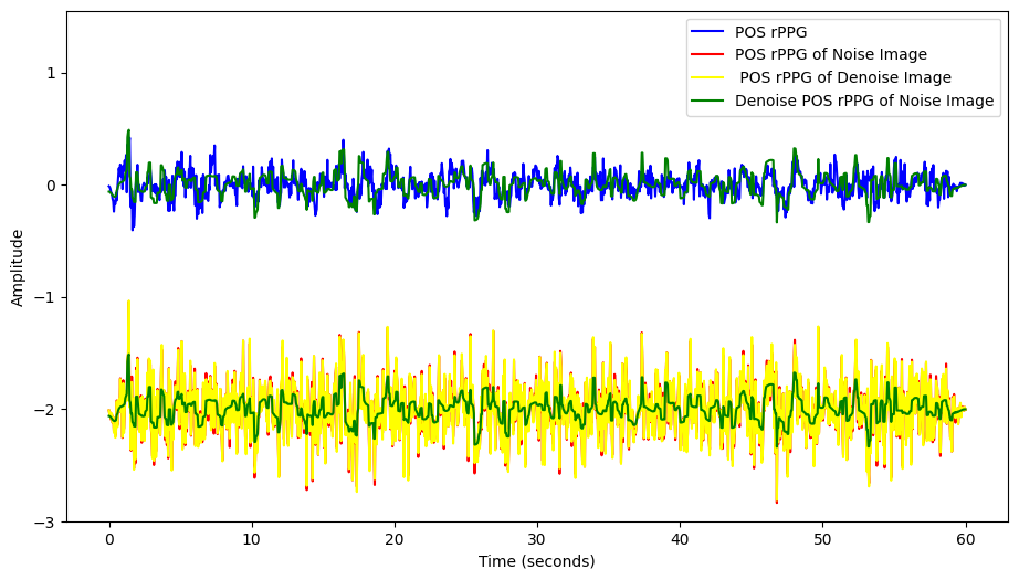
Figure S1: Examples of four types of POS rPPG signals

Table S1: Heart Rate Estimation Errors: Baseline, Noise, and Denoising Datasets

		Dataset
Trans.	rPPG Meth.	COHFACE		LGI-PPGI		MAHNOB		PURE		UBFC-rPPG		UCLA-rPPG		UBFC-Phys
		MAE	PCC	MAE	PCC	MAE	PCC	MAE	PCC	MAE	PCC	MAE	PCC	MAE	PCC
	NLM
BS	OMIT	11.24	0.27	8.79	0.73	36.93	0.02	1.43	0.98	3.49	0.94	3.65	0.56	13.30	0.27
Noise		41.58	0.10	17.10	0.50	44.83	0.02	17.62	0.35	13.62	0.54	20.16	0.27	18.81	0.19
TVI		41.31	0.10	16.96	0.51	44.65	0.03	17.68	0.33	13.76	0.54	20.16	0.28	19.00	0.19
TVS		15.28	0.08	13.86	0.53	33.81	0.04	8.20	0.62	12.24	0.54	7.33	0.43	14.44	0.20
BS	CHROM	12.39	0.21	10.87	0.60	37.13	-0.02	1.42	0.98	3.05	0.97	3.76	0.59	13.65	0.25
Noise		48.04	0.09	19.90	0.42	46.24	0.02	19.58	0.33	17.12	0.44	19.85	0.28	19.49	0.20
TVI		47.77	0.09	19.67	0.42	45.52	0.03	19.45	0.32	17.72	0.43	20.07	0.28	19.52	0.20
TVS		37.09	0.10	18.89	0.40	43.82	0.02	16.73	0.35	15.70	0.45	16.74	0.28	18.64	0.19
BS	POS	11.58	0.27	6.05	0.84	36.55	0.03	1.25	0.99	2.74	0.99	3.06	0.65	13.69	0.25
Noise		42.75	0.10	16.50	0.54	44.55	0.03	18.30	0.35	13.00	0.53	21.44	0.27	19.67	0.20
TVI		42.71	0.08	16.61	0.52	44.38	0.03	18.49	0.34	12.91	0.55	21.00	0.27	19.95	0.19
TVS		16.91	0.13	13.80	0.55	37.52	0.01	13.02	0.35	13.24	0.49	10.72	0.28	15.47	0.18
	DLM
BS	Efficient Phys	17.46	0.06	18.33	0.37	38.35	-0.03	10.12	0.50	7.73	0.69	7.99	0.37	15.93	0.17
Noise		23.10	0.00	27.27	0.08	40.04	-0.04	27.07	-0.01	32.81	-0.02	26.06	0.05	23.60	-0.01
TVI		21.35	-0.01	25.36	0.19	40.08	-0.03	23.07	0.06	30.80	0.03	20.83	-0.03	22.55	0.01
TVS		17.35	-0.02	24.97	0.11	38.92	0.00	21.21	0.01	32.10	-0.02	20.50	0.03	22.05	-0.02
BS	Contrast Phys	9.67	0.22	13.86	0.50	46.52	0.06	11.63	0.59	3.72	0.94	7.13	0.40	16.87	0.17
Noise		10.10	0.10	14.06	0.51	46.58	0.08	26.31	0.16	6.11	0.81	15.11	0.17	21.33	0.07
TVI		10.43	0.13	14.51	0.50	46.54	0.07	25.73	0.19	6.63	0.79	15.24	0.13	22.44	0.06
TVS		10.15	0.10	14.46	0.48	46.43	0.08	25.55	0.16	6.25	0.81	14.14	0.20	20.39	0.09
The term BS represents the normal image at 72x72 pixels, the bold represents the deteriorated result needing improvement, while the underline marks enhancements in both metrics compared to the bold.

S2 Visual Occlusion and Mitigation

This section provides supplementary information regarding visual occlusion mitigation involving sunglasses and the combination of sunglasses and facemasks. Figures S2 respectively illustrate each stage of the process applied to facial images, demonstrating the mitigation methods for occlusions involving various types of eye and face combinations.

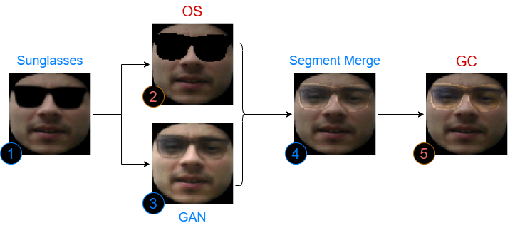
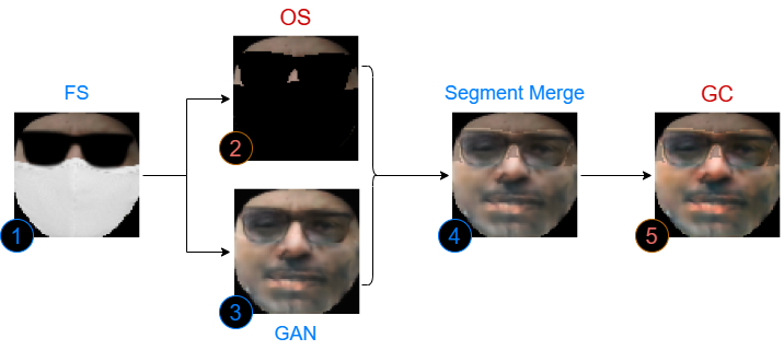
Figure S2: Illustrations demonstrating sunglasses and both visual occlusion mitigation. 1) Occluded image, 2) Original skin image, 3) GAN generated image, 4) Merged image of original and generated skin, 5) Merged image with color transfer from real to generated skin.

For heart rate estimation, as illustrated in Table S2, the combined presence of facemasks and sunglasses surprisingly did not significantly impact the accuracy of heart rate estimation as anticipated. In fact, some results even showed improvement compared to those obtained with the facemask alone. This unexpected outcome could potentially be attributed to the contrasting colors of the mask and sunglasses, although not purely black or white, still interact in a complementary manner within a certain range.

Table S2: Heart Rate Estimation Errors: Baseline, Occlusion, and Mitigating Datasets

		Dataset
Trans.	rPPG Meth.	COHFACE		LGI-PPGI		MAHNOB		PURE		UBFC-rPPG		UCLA-rPPG		UBFC-Phys
		MAE	PCC	MAE	PCC	MAE	PCC	MAE	PCC	MAE	PCC	MAE	PCC	MAE	PCC
	NLM
BS	OMIT	11.24	0.27	8.79	0.73	36.93	0.02	1.43	0.98	3.49	0.94	3.65	0.56	13.30	0.27
FS		19.76	0.08	9.37	0.76	36.72	0.07	2.83	0.89	11.74	0.42	6.46	0.43	15.33	0.21
GC		20.66	0.11	10.40	0.70	36.80	0.10	8.04	0.59	9.80	0.51	9.38	0.36	14.85	0.20
OS		17.10	0.14	7.71	0.79	36.30	0.08	2.22	0.93	5.22	0.73	6.28	0.41	14.13	0.24
BS	CHROM	12.39	0.21	10.87	0.60	37.13	-0.02	1.42	0.98	3.05	0.97	3.76	0.59	13.65	0.25
FS		18.32	0.09	9.40	0.73	36.94	0.06	2.79	0.90	12.31	0.44	7.28	0.42	15.07	0.22
GC		20.10	0.09	13.08	0.59	37.30	0.06	8.57	0.61	9.58	0.58	10.44	0.33	14.63	0.23
OS		15.67	0.11	9.35	0.72	36.29	0.07	1.96	0.95	5.77	0.76	6.78	0.45	14.10	0.24
BS	POS	11.58	0.27	6.05	0.84	36.55	0.03	1.25	0.99	2.74	0.99	3.06	0.65	13.69	0.25
FS		17.63	0.12	6.80	0.84	36.08	0.07	2.04	0.95	5.10	0.82	6.09	0.43	14.39	0.23
GC		21.61	0.09	9.79	0.70	36.82	0.10	8.47	0.58	6.63	0.72	9.49	0.34	14.64	0.23
OS		16.66	0.13	7.42	0.78	35.98	0.07	2.23	0.93	3.30	0.95	6.10	0.45	14.01	0.25
	DLM
BS	Efficient Phys	17.46	0.06	18.33	0.37	38.35	-0.03	10.12	0.50	7.73	0.69	7.99	0.37	15.93	0.17
FS		22.14	0.00	27.78	0.04	38.56	-0.01	22.03	0.07	29.31	0.10	21.65	0.00	22.93	0.02
GC		21.56	-0.02	24.50	0.12	38.03	-0.01	24.84	0.01	31.11	0.02	21.53	0.04	23.42	0.01
OS		47.86	0.01	62.17	0.10	51.81	-0.07	105.76	-0.05	71.21	-0.02	104.76	0.01	103.32	0.01
BS	Contrast Phys	9.67	0.22	13.86	0.50	46.52	0.06	11.63	0.59	3.72	0.94	7.13	0.40	16.87	0.17
FS		12.76	0.03	18.36	0.28	46.95	0.04	30.92	0.00	12.50	0.44	21.60	0.05	24.07	0.08
GC		11.60	0.00	18.59	0.29	47.34	0.08	31.06	0.17	12.74	0.40	22.88	0.08	28.36	0.03
OS		11.42	0.06	19.89	0.21	46.51	0.08	29.35	0.11	14.76	0.28	22.23	0.03	27.97	0.05
The term ”BS” stands as the baseline result for images sized 72x72 pixels without occlusion, the bold represents the result of visual occlusion, while the underline marks enhancements in both metrics compared to the bold. ”FS” indicates the presence of facemask and sunglasses. ”OS” refers to the original skin region method, while ”GC” represents GAN-OS with the color transfer method.

In terms of the mitigation strategy for heart rate estimation with NLM, in cases of facemasks and sunglasses combined, the GAN method exhibited improvement in a few datasets, while the rest performed worse than the occluded images. Surprisingly, the original skin region approach with little skin region remains demonstrated a slight improvement in some datasets and methods. Regarding the mitigated strategy for heart rate estimation with DLM, for facemasks, the two DLM methods demonstrated different trends. While ContrastPhys exhibited a slight improvement in some datasets with both mitigate methods, EfficientPhys performed poorly and only showed a very slight increase in some datasets with the GANs method.

References

-
[1]
S. van der Walt, J. L. Schönberger, J. Nunez-Iglesias, F. Boulogne, J. D. Warner, N. Yager, E. Gouillart, T. Yu, the scikit-image contributors, scikit-image: image processing in Python, PeerJ 2 (2014) e453.
doi:10.7717/peerj.453.
URL https://doi.org/10.7717/peerj.453