CoolWalks: Assessing the potential of shaded routing
for active mobility in urban street networks

Abstract

Walking is the most sustainable form of urban mobility, but is compromised by uncomfortable or unhealthy sun exposure, which is an increasing problem due to global warming. Shade from buildings can provide cooling and protection for pedestrians, but the extent of this potential benefit is unknown. Here we explore the potential for shaded walking, using building footprints and street networks from both synthetic and real cities. We introduce a route choice model with a sun avoidance parameter $\alpha$ and define the CoolWalkability metric to measure opportunities for walking in shade. We derive analytically that on a regular grid with constant building heights, CoolWalkability is independent of $\alpha$, and that the grid provides no CoolWalkability benefit for shade-seeking individuals compared to the shortest path. However, variations in street geometry and building heights create such benefits. We further uncover that the potential for shaded routing differs between grid-like and irregular street networks, forms local clusters, and is sensitive to the mapped network geometry. Our research identifies the limitations and potential of shade for cool, active travel, and is a first step towards a rigorous understanding of shade provision for sustainable mobility in cities.

Introduction

To make cities more sustainable and liveable, it is of utmost importance to reduce vehicular traffic and associated car harm [1, 2], and to promote active mobility like walking and cycling [3]. Active mobility can, for example, be fostered through implementing 15-minute cities, low-traffic neighborhoods, or by improving bicycle infrastructure [4, 5, 6, 7, 8, 9]. However, such efforts are only effective if people find the street environment safe and comfortable. An important factor for safety and comfort, apart from low vehicular traffic, is protection from high temperatures and sun exposure. The climate crisis unfortunately comes with global warming and growing temperature variations that create an increasingly hostile outdoor environment [10]. Cities are especially prone to heat island effects which cause excess deaths from heat exposure [11]. To combat these effects, preventing the causes of the climate crisis should be the top priority [12]. Nevertheless, ensuring acceptable standards of living in cities amid rising global temperatures and increasing urbanization also calls for the urgent exploration of adaptation strategies.

One such adaptation strategy is the provision of shade, to allow pedestrians and cyclists to avoid time spent in direct sunlight. Shade provision is frequently overlooked in urban planning and climate-change mitigation strategies, despite being one of the most efficient and cost-effective ways to reduce heat-related health risks outdoors [13]. Improving shade provision has the dual benefit of minimizing the harmful impacts of a changing climate while stimulating sustainable modes of mobility that do not contribute to further climate change [14]. Although there is an increasing body of research addressing active mobility [15, 16], the provision of shade for active mobility is barely explored. In this paper, we start addressing this gap by studying the complex relation between shade distributions and the geometry of buildings and street networks, shedding light on the built environment’s effect on shade availability for pedestrians.

The cooling benefits from shade in cities have previously been covered from diverse perspectives such as urban planning [17, 14], engineering [18, 19, 20], or public health [21, 22]. The latter has established that shade provides relief for temperature-related health issues and contributes strongly to a decrease in physiological equivalent temperature [23, 24, 13], increasing the subjective well-being when traveling. Furthermore, mobile phone app prototypes have been developed that implement shade-optimized routing, showcasing the feasibility of a practical application [25, 26, 27], but without systematic explorations of the potential for walking or cycling in shade.

Pedestrians and cyclists are much more exposed to their surrounding environments than motorists [28, 29]. Most routing for active mobility thus considers not just travel time or distance, but also, for example, traffic safety [30], land use [29], the attractiveness of the surroundings, or avoiding smells, noises, or other unpleasant sensory experiences [31, 32]. However, considering shade for pedestrian routing is spatiotemporally more intricate, since shade availability depends on the interplay between sidewalk network topology and the built environment, together with a dynamic dependence on the time of day.

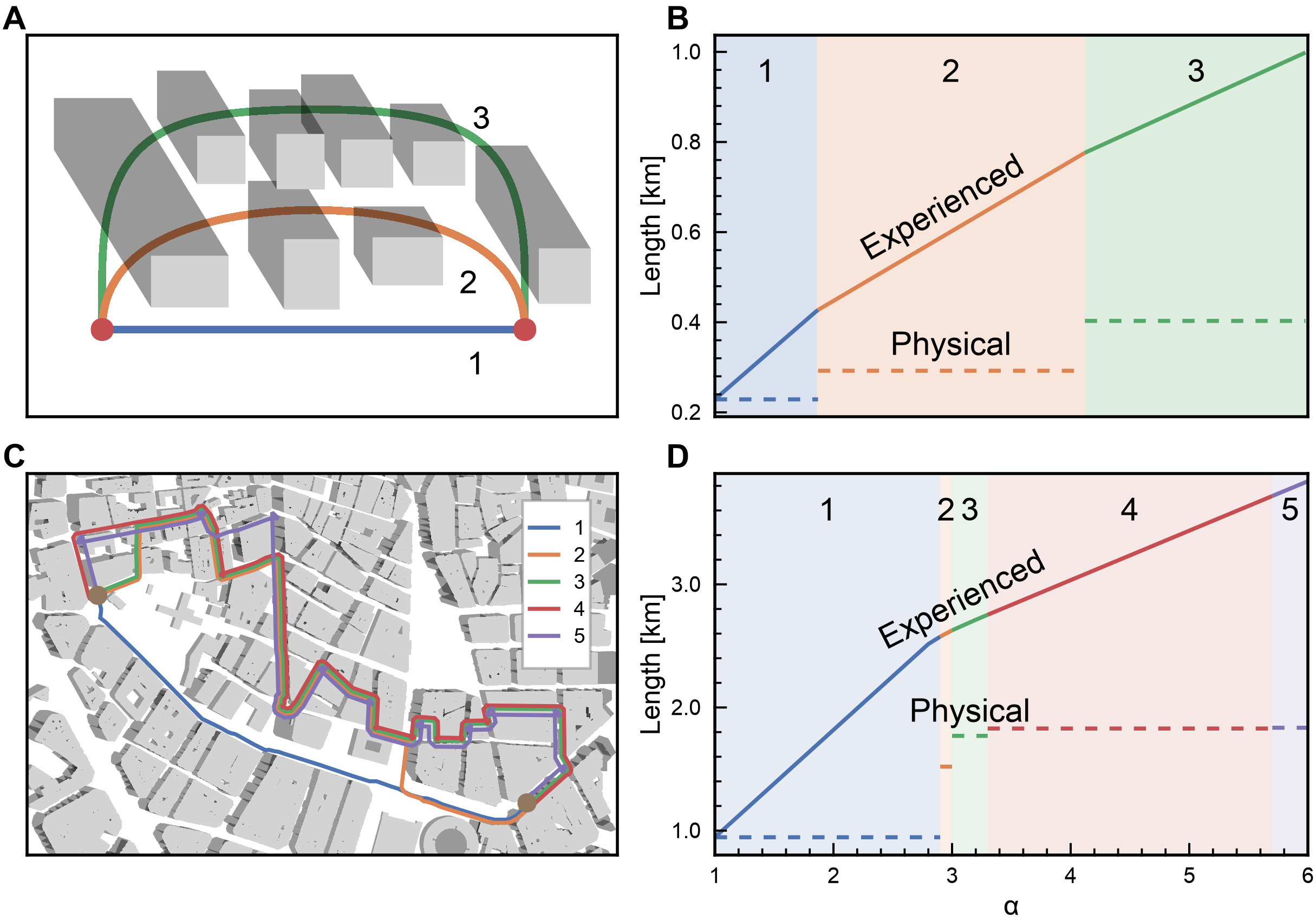
Figure 1: Higher sun avoidance $\alpha$ implies choice of routes that are not physically shortest but that minimize experienced length. A: Example of three different links connecting two nodes in the street network, from shortest and least shaded (1, blue) to longest and most shaded (3, green). B: The choice of which link to take depends on the pedestrian’s sun avoidance $\alpha$. Increasing sun avoidance increases the experienced length because walking in the sun becomes less tolerable. At the threshold between different regimes, for example 1 (blue) to 2 (orange), the experienced length of the shaded link 2 becomes shorter than the experienced length of sunny link 1, implying a preference for link 2 despite longer physical length (dashed orange line). C,D: Generalization from links to shortest paths with an example of five routes.

To contribute to the fields of active mobility and climate adaptation research, we introduce a route choice model for walking with a sun aversion parameter $\alpha$ and a CoolWalkability metric that operationalizes the potential for shaded routing given an amount and spatial distribution of shade. By studying this metric we reveal the nontrivial impact of street networks and building height distributions on shade provision for active mobility. We measure CoolWalkability for cities with different urban forms and street networks, from grid-like to irregular: Manhattan, Barcelona, Valencia. We introduce diurnal (daily) CoolWalkability profiles and phase portraits to visualize the progression of CoolWalkability in cities over the day. These tools allow us to disentangle the effects of building heights and street geometry, and to compare Manhattan’s empirical data to the analytical solution for a corresponding regular grid.

We find that the analytic grid solution is independent of an individual’s sun aversion $\alpha$, meaning that individuals are not able to minimize time walking in the sun between an origin-destination pair on a perfect grid. However, the slight variations in Manhattan’s building heights and street geometry improve the CoolWalkability compared to the exact grid with constant building height, yielding potential benefits for shade-seeking individuals. Moreover, by comparing grid-like cities like Manhattan with more irregular street geometries from Barcelona and Valencia we uncover different classes of diurnal CoolWalkability profiles that are spatially clustered, meaning that shade availability varies substantially between different parts of the cities. Finally, we discuss the effect of network geometry on the CoolWalkability and compare results between sidewalk and bicycle networks. Understanding how, where, and why the built environment contributes to shade availability are important first steps in adapting cities to a hotter climate and supporting active mobility throughout the year.

Model and metrics

In this section Model and metrics we first define our route choice model, then the corresponding CoolWalkability metric.

Route choice model with sun aversion $\alpha$

How a shade-seeking pedestrian selects their routes when traversing a city depends on the available shade along the streets. They might choose to walk farther than the shortest path but with reduced sun exposure, trading a shorter total distance travelled for a longer distance travelled in the shade. We therefore express the problem of finding the best shaded route in terms of a shortest path problem on the street network $G=(V,E)$ with edge lengths given by the experienced length

$$\lambda_{ij}=\alpha\cdot l^{\raisebox{0.0pt}{\scalebox{0.75}{\sun{}}}{}}_{ij}+l^{\raisebox{0.91003pt}{\scalebox{0.6}{\newmoon{}}}{}}_{ij}$$ (1)

where $l^{\raisebox{0.0pt}{\scalebox{0.75}{\sun{}}}{}}_{ij}$ and $l^{\raisebox{0.91003pt}{\scalebox{0.6}{\newmoon{}}}{}}_{ij}$ are the physical lengths in the sun or shade on the street segment $(i,j)$ connecting intersections $i$ and $j$, respectively. The parameter $\alpha\in\left[1,\infty\right)$ captures the sun aversion of a pedestrian: A constant distance travelled in the sun is experienced as $\alpha$ times as long as the same distance travelled in shade. An example of the effect of $\alpha$ is shown in Fig. 1A,B, where the blue link is the shortest but most sun-exposed link preferred by individuals who are not sun-averse (low $\alpha$), while the other links are longer but less sun-exposed preferred by individuals with sun aversion (higher $\alpha$).

Generalizing the experienced length of a link, we define the experienced length of a path $\Lambda^{\alpha}_{i\rightarrow j}$ as

$$\Lambda^{\alpha}_{i\rightarrow j}\left(\Pi_{i\rightarrow j}\right)=\sum_{ab\in\Pi_{i\rightarrow j}}\lambda_{ab}$$ (2)

where $\Pi_{i\rightarrow j}=\left(i\rightarrow k_{1},k_{1}\rightarrow k_{2},...,k_{N-1}\rightarrow j\right)$ is a path of length $N$ between $i$ and $j$.

For constant time of day and $\alpha$, we assume that a pedestrian minimizes their experienced path length $\Lambda^{\alpha}_{i\rightarrow j}$ choosing the path

$$\Pi^{*}_{i\rightarrow j}=\mathrm{argmin}\left(\Lambda^{\alpha}_{i\rightarrow j}(\Pi_{i\rightarrow j})\right)$$ (3)

over all possible paths $\left\{\Pi_{i\rightarrow j}\right\}$ connecting node $i$ to node $j$.

In this context, $\alpha$ is an upper bound on the maximal increase of the physical length of the shortest path, compared to the physically shortest path at $\alpha=1$. For example, an $\alpha=1.5$ means that a pedestrian tolerates an increase in path length of up to 50%. Figure 1C,D illustrates how different values of $\alpha$ imply different selected paths through a city.

The exact values of $\alpha$ are not easy to determine empirically, as they might depend on various individual preferences like heat resilience or time constraints, and on local or temporal factors like surface, the height of the sun, or wind conditions. Pedestrians are in general willing to endure detours for a variety of reasons [33, 30] compared to the physically shortest path. We therefore set the studied sun aversions to $\alpha\in\left\{1.1,1.25,1.5,2,4,10\right\}$, capturing both realistic values ($\alpha\leq 1.5$) and extreme values ($\alpha\gg 1$) for a comprehensive exploration of the parameter space.

For all shortest-path calculations, we consider fixed times during the 21^st of July 2023, not including possible changes in shade during any trip. This simplification, together with the local weights of experienced edge lengths $\lambda_{ij}$, enables us to efficiently calculate the shortest path for various scenarios using Dijkstra’s shortest path algorithm [34].

Defining CoolWalkability

At each point in time $t$, the shadow fraction $S_{ij}(t)$ of a street-segment $(i,j)$ is defined as

$$S_{ij}(t)=\frac{l^{\raisebox{0.91003pt}{\scalebox{0.6}{\newmoon{}}}{}}_{ij}{}(t)}{l_{ij}{}},$$ (4)

denoting the fraction of the segment covered in shade. Similarly, the global shadow fraction $S(t)$ denotes the total shaded length available in the city at time $t$, normalized by the full length of all streets

$$S(t)=\frac{\sum\limits_{(i,j)\in E}l^{\raisebox{0.91003pt}{\scalebox{0.6}{\newmoon{}}}{}}_{ij}{}(t)}{\sum\limits_{(i,j)\in E}l_{ij}{}}$$ (5)

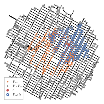
Figure 2: Study area definition. We use a subgraph of the Manhattan street network centered around Times Square; similar subgraphs are extracted from the centers of Barcelona and Valencia. Each considered source node $i\in V_{src}$ (orange) lies within $800\text{\,}\mathrm{m}$ of the center and has a set of reachable nodes $V_{dst}(i)$, here highlighted in blue for one example node $i$ (red). We limit the number of reachable nodes to a maximum distance of $800\text{\,}\mathrm{m}$ on the street network, to consider realistic walking distances. To avoid edge effects caused by cutting the network from the full road network, we include all nodes within $1600\text{\,}\mathrm{m}$ of the center. The nodes used in our analysis are therefore the source nodes together with all the nodes in the padding-area (grey).

This global shadow fraction is a baseline performance measure for a given city which consists of a street network and the associated buildings. We then define the global CoolWalkability $C^{\alpha}$(t) as

$$C^{\alpha}(t)=\frac{\sum\limits_{i\in V_{\mathrm{src}},j\in V_{\mathrm{dst}}(i)}\left(\Lambda^{\alpha,*}_{i\rightarrow j}(0)-\Lambda^{\alpha,*}_{i\rightarrow j}\left(\left\{S_{ab}(t)\right\}\right)\right)}{\sum\limits_{i\in V_{\mathrm{src}},j\in V_{\mathrm{dst}}(i)}\left(\Lambda^{\alpha,*}_{i\rightarrow j}(0)-\Lambda^{\alpha,*}_{i\rightarrow j}(1)\right)}$$ (6)

where $\Lambda^{\alpha,*}_{i\rightarrow j}$ is the experienced length of the shortest path between $i$ and $j$, expressed as a function either of the shadow fraction $\left\{S_{ab}(t)\right\}$ at time $t$ or at constant shadow fractions $S_{ij}=0$ or $S_{ij}=1$ for all edges $(i,j)\in E$, respectively, representing the worst and best case of shade coverage for the city. The CoolWalkability thus represents how much shorter all experienced trip-lengths are, compared to the trip lengths in the worst-case scenario with no shade available at all. To make these results comparable between various cities, this value is then normalized by the maximal difference in all experienced trip lengths. CoolWalkability is inspired by a recent definition of bikeability [7].

We only consider destinations $V_{\mathrm{dst}}(i)=\left\{j\in V\,\middle|\,\Lambda^{1,*}_{i\rightarrow j}<$800\text{\,}\mathrm{m}$\right\}$ to emulate a limited range of activity for each pedestrian. This restriction also makes the error negligible from assuming a constant sun position for the duration of a trip. Figure 2 shows the different parts of the summation setup on the street graph of Manhattan. With an average speed of $5\text{\,}\mathrm{k}\mathrm{m}\mathrm{/}\mathrm{h}$, it would take a pedestrian around $10\text{\,}\min$ to complete the longest allowed trip, an interval in which sun position and shade are assumed to not change noticeably.

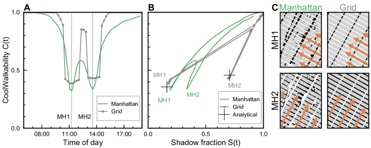
Figure 3: Comparing CoolWalkability of Manhattan with a synthetic grid shows similarities but also crucial differences. A: We introduce the diurnal Coolwalkability profile (here shown for 2023-06-21, and $\alpha=1.5$). It shows two characteristic dips for Manhattan (green) due to the two Manhattanhenge events MH1 and MH2 at 11:05 and 13:25, respectively, where the sun is aligned with the grid. The dips are also present in the synthetic grid (grey), but less pointed. B: We introduce the diurnal CoolWalkability phase portrait. It shows CoolWalkability versus shadow fraction, as functions of time, revealing larger differences. Manhattan’s portrait (green) is relatively smooth due to slight imperfections in its grid structure and heterogeneous building heights, while the grid’s portrait (grey) jumps discontinuously due to its perfect symmetries and constant building heights. The grid’s analytical solution of Manhattanhenges (black crosses) fits well with the numerical simulation. C: Illustration of the two Manhattanhenge events MH1 and MH2 for Manhattan and the synthetic grid. Grey polygons denote building footprints, black polygons their shadows, orange arrows the direction of sun rays.

Data

In this section Data we outline the data of street networks and buildings to which we apply our routing model. We focus on subsections from Manhattan, Barcelona, and Valencia. The street networks are taken from OpenStreetMap (OSM) [35], while the building data were provided by the New York City Office of Technology and Innovation [36] for Manhattan and by the General Directorate for Cadastre of Spain [37] for Barcelona and Valencia.

The sidewalk networks available via OSM can be highly detailed, often including sidewalks on both sides of a street as well as the multiple ways in which pedestrians can cross a street, for example around intersections [38]. While these higher resolution networks are generally favorable for analyzing pedestrian mobility, OSM data availability depends on the activity of the local OSM communities [39, 40, 41]. Despite increasing crowd-sourced and remote sensing efforts to collect better data, accurate high-resolution sidewalk networks are currently not available in OSM for most cities around the world [38]. As a useful proxy for sidewalk networks, we therefore consider bicycle networks, which we define as all road infrastructure that can legally be used by cyclists. Following this definition, bicycle networks are well mapped in general [42, 43] because they consist to a large extent of mostly well mapped road networks [44]. Bicycle networks come with the additional benefit of small size compared to the full sidewalk networks, with comparable spatial coverage. Further, it is reasonable to assume that the vast majority of the bicycle network can also be reached by pedestrians – we support this assumption by comparing the bicycle and sidewalk networks for the three study areas, finding that more than $80\text{\,}\mathrm{\char 37\relax}$ of the OSM ways which make up the bicycle network are contained in the respective sidewalk network. The bicycle network is thus a reasonable proxy for the sidewalk network in areas that lack a detailed mapping of sidewalks. It also reduces computational complexity, as shown for the study areas in Table 1.

Following this argument we focus on the bicycle networks, interpreting them as simplified versions of the full pedestrian networks. As pedestrians do not need to adhere to one-way streets, we ignore edge directions by adding all non-existent reverse edges to the graphs of both network types. We compare the differences between these two networks in section Network geometry matters.

	Manhattan		Barcelona		Valencia
	cycle	walk	cycle	walk	cycle	walk
Nodes	$1506$	$8702$	$2780$	$10\,975$	$3156$	$8052$
Edges	$4114$	$27\,200$	$8572$	$33\,402$	$9456$	$23\,858$
Length [km]	$292$	$845$	$441$	$865$	$463$	$693$
Buildings	$6385$		$14\,479$		$9483$

Table 1: Datasets studied in this project.

Given sparse availability of full 3D building data, and for computational simplicity, we handle building data following the 2.5D standard, i.e. consisting of a footprint-polygon and a singular height value which is simplified as constant across the whole building.

In addition to the empirical data, we consider two types of synthetic cities. On one extreme, we study cities based on an ideal, regular grid with cell edge lengths $l_{a}$ and $l_{b}$. On the other extreme, we construct cities from the Poisson-Voronoi tesselation [45]. In this model, seed-points are first distributed randomly, then Voronoi cells are created around them, and the cell edges model the city’s streets. For each of these synthetic cities we either assume a constant height across all buildings, or we sample the building heights from the empirical building height distributions. See Supplementary Note 2 for more details on data generation and processing.

Results

Before analyzing empirical data from real-world cities, we solve the case of the grid street network analytically, setting the theoretical expectation for CoolWalkability in grid-like cities. We then introduce the diurnal CoolWalkability profile and phase portrait, allowing us to compare deviations of this expectation with a synthetic grid and with the empirical results in Manhattan. This comparison untangles the different factors that cause these deviations: Grid deviations and non-uniform building height distribution. After the grid analysis, we incorporate Barcelona and Valencia, two cities with a more irregular street geometry. Last, after observing global differences in CoolWalkability, spatial cluster analysis also reveals local differences between grid-like and irregular network structures.

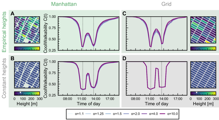
Figure 4: Disentangling the effects of building height distribution and street geometry on Coolwalkability. Multiple curves shown in diurnal profiles correspond to different sun avoidance values $\alpha$ – the curves mostly overlap, showing independence of Coolwalkability from $\alpha$, as proven analytically for the grid. All diurnal profiles shown for 2023-06-21. A: Left: Zoom into Manhattan’s building footprints. Right: diurnal Coolwalkability profile. B: Left: Zoom into Manhattan’s building footprints at constant height, set as the average $71\text{\,}\mathrm{m}$ of empirical building heights. Right: The corresponding diurnal Coolwalkability profile. Due to loss of building height heterogeneity, the Manhattanhenge dips are slightly less pointy. C: Right: Zoom into the grid with empirical building footprints taken from Manhattan. Left: the corresponding diurnal Coolwalkability profile. Keeping building height heterogeneity but changing from empirical street network to grid implies only slight differences in diurnal Coolwalkability. D: Right: Zoom into the grid’s building footprints at constant height, set as the average $71\text{\,}\mathrm{m}$ of empirical building heights. Left: the corresponding diurnal Coolwalkability profile. Due to loss of building height heterogeneity and the change to a grid, the Manhattanhenge dips are considerably broader and less pointy.

CoolWalkability on a grid is independent of sun avoidance $\alpha$

A theoretical approximation of a city with a grid-like street network like Manhattan is a regular grid consisting of rectangles with edge lengths $l_{a}$ and $l_{b}$, and buildings of a constant height, which are inset from the streets by a distance $w$. On this grid, we derive the CoolWalkability analytically (full derivation in Supplementary Note 1) as a function of the length of shade $l^{\raisebox{0.91003pt}{\scalebox{0.6}{\newmoon{}}}{}}_{a}$ and $l^{\raisebox{0.91003pt}{\scalebox{0.6}{\newmoon{}}}{}}_{b}$ on the edges:

$$C^{\alpha}\left(l^{\raisebox{0.91003pt}{\scalebox{0.6}{\newmoon{}}}{}}_{a},l^{\raisebox{0.91003pt}{\scalebox{0.6}{\newmoon{}}}{}}_{b}\right)=\frac{l_{b}\cdot l^{\raisebox{0.91003pt}{\scalebox{0.6}{\newmoon{}}}{}}_{a}+l_{a}\cdot l^{\raisebox{0.91003pt}{\scalebox{0.6}{\newmoon{}}}{}}_{b}}{2l_{a}l_{b}}$$ (7)

This expression is independent of $\alpha$, showing that highly symmetric cities offer pedestrians no choice for more shaded routes, no matter how high their sun aversion. Conversely, the fraction of total street length in shade is given by

$$S\left(l^{\raisebox{0.91003pt}{\scalebox{0.6}{\newmoon{}}}{}}_{a},l^{\raisebox{0.91003pt}{\scalebox{0.6}{\newmoon{}}}{}}_{b}\right)=\frac{l^{\raisebox{0.91003pt}{\scalebox{0.6}{\newmoon{}}}{}}_{a}+l^{\raisebox{0.91003pt}{\scalebox{0.6}{\newmoon{}}}{}}_{b}}{l_{a}+l_{b}}$$ (8)

which, unlike Eq. 7, is symmetric in both its arguments, showing how the same total shadow fraction $S$ may lead to different CoolWalkabilities, depending not only on the distribution of said shade but also on the underlying geometry. For example, if $l^{\raisebox{0.91003pt}{\scalebox{0.6}{\newmoon{}}}{}}_{a}=x$ and $l^{\raisebox{0.91003pt}{\scalebox{0.6}{\newmoon{}}}{}}_{b}$=0, we get $S\left(x,0\right)=S\left(0,x\right)$ but $C^{\alpha}\left(x,0\right)=\frac{l_{b}\cdot x}{2l_{a}l_{b}}\neq\frac{l_{a}\cdot x}{2l_{a}l_{b}}=C^{\alpha}\left(0,x\right)$ if $l_{a}\neq l_{b}$.

Diurnal CoolWalkability profile and phase portrait reveal differences between Manhattan and grid

As a tool to visually study CoolWalkability over the course of a day, we introduce the diurnal CoolWalkability profile and phase portrait. Figures 3A and B show these visualization methods, respectively, comparing the results using empirical data from Manhattan with numerical results in a synthetic city. The synthetic city is based on a regular grid as introduced in the previous section, with parameters chosen to fit the underlying grid structure of Manhattan. Each grid cell has edge lengths of $l_{a}=$270\text{\,}\mathrm{m}$$ and $l_{b}=$80\text{\,}\mathrm{m}$$, and is rotated by $61\text{\,}\mathrm{\SIUnitSymbolDegree}$ counterclockwise to align with the street grid of Manhattan. The buildings are inset by $w=$11.5\text{\,}\mathrm{m}$$ and have a constant height of $71\text{\,}\mathrm{m}$, the area-weighted average of the building heights in the Manhattan dataset.

Comparing the diurnal CoolWalkability profiles, Fig. 3A, we find a generally similar shape, both showing similar dips around 11:05 and 13:25, caused by the characteristic “Manhattanhenge” events where the sun shines down the urban canyons either from the south-east (MH1) or south-west (MH2) direction. In both events, the CoolWalkability is roughly similar between the two dips, slightly higher at MH2. In the synthetic grid (grey), the CoolWalkability shows discontinuities, caused by the high symmetry of the gridded city, where all shadows sweep over the streets at the same time. These discontinuities disappear for the empirical data (green). We explore this smoothening in the next section.

When comparing the CoolWalkability against the shadow fraction in a diurnal phase portrait, Fig. 3B, we see more substantial differences, especially around the second Manhattanhenge event MH2. Here, the shadow fraction on the grid is considerably larger than the one in Manhattan, without showing a proportional increase in CoolWalkability. This observation is consistent with the theoretical predictions from Eqs. 7 and 8 because $C^{\alpha}\left(l^{\raisebox{0.91003pt}{\scalebox{0.6}{\newmoon{}}}{}}_{a},0\right)\approx C^{\alpha}\left(l_{a},0\right)=C^{\alpha}\left(0,l_{b}\right)\approx C^{\alpha}\left(0,l^{\raisebox{0.91003pt}{\scalebox{0.6}{\newmoon{}}}{}}_{b}\right)$ for $w\ll l_{a}$ and $w\ll l_{b}$.

Around MH2, Manhattan has much less shade available compared to the grid but is still able to provide about as good a CoolWalkability as the grid. In general, the empirical curve (green) runs to the left or above the grid curve (grey) during corresponding times of the day, implying a better potential use of shade for walking than expected for a perfect grid with constant building heights. This situation is different for Barcelona and Valencia, which are less grid-like and have lower, more uniform building heights, therefore not featuring distinct “henge” events, see Supplementary Figures SI1 and SI2.

Empirical building heights smoothen diurnal profiles

To untangle the different effects leading to deviations between empirical and synthetic data, as just observed in Fig. 3B, we investigate the impact of a constant building height distribution, by running the same study on Manhattan but with constant building heights of $71\text{\,}\mathrm{m}$, and on the grid with building heights randomly drawn from the area-weighted distribution observed in Manhattan. The results of this experiment are shown in Fig. 4. Going from the fully empirical Manhattan (Fig. 4A) to the case of Manhattan with constant building heights (Fig. 4B), we find the dips around the two Manhattanhenges to widen and to increase their CoolWalkability values slightly. Also, the flanks dropping in to MH1 and leading out of MH2 steepen. Going from Manhattan with constant building heights (Fig. 4B) to the most synthetic case of a grid with constant building heights (Fig. 4D) iterates the same effect changes: The dips plateau and widen, discontinuities and slopes increase. The effect of going from the fully empirical Manhattan (Fig. 4A) to the grid with empirical heights (Fig. 4C) is mostly a slight increase in CoolWalkability values, but keeping a similar pointedness of Manhattanhenge dips. The biggest effect is observed in the grid case, going from empirical to constant heights (Fig. 4C to D). The two dips go from sharp to two plateaus stretched over around 1.5 hours each.

To summarize, going from empirical to constant building heights has a stronger impact on diurnal CoolWalkability profiles than going from Manhattan to the perfect grid. Manhattan’s grid imperfections have a negligible influence on CoolWalkability. An implied consequence for future modeling efforts is to prefer approximating a grid-like network with a perfect grid than to neglect the heterogeneous distribution of building heights. For all these cases, we also observe little to no $\alpha$-dependence of the profiles (they mostly overlap), further showing how there are nearly no relevant choices to be made by pedestrians in such grid-like networks.

CoolWalkability clusters locally

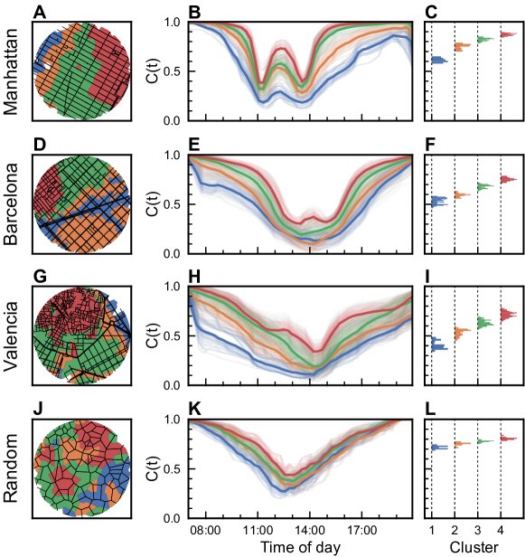
Figure 5: Spatial clustering by CoolWalkability leads to areas with different profiles. From top to bottom, we study the cities Manhattan, Barcelona, Valencia, and the random null model (Poisson-Voronoi). Left column: Clustering local Coolwalkability of each node in the street network leads to spatial clusters of similar CoolWalk potential. Middle column: The diurnal profiles of these clusters display high variations within each city and between different cities. In particular, the more organic, least grid-like areas (red curves) display the highest potential. K: The null model shows the baseline of small variation. Right column: the distributions of the time average of each diurnal profile within each cluster illustrate the large potential differences in empirical street networks. L: These differences are negligible in the null model.

The global CoolWalkability is aggregated over the whole study area, neglecting spatial heterogeneities within cities which might affect CoolWalkability locally. To study the impact of the geometric variations in building and street geometry, we calculate the local CoolWalkability $C^{\alpha}_{i}$(t) for each vertex $i\in V_{src}$ as

$$C^{\alpha}_{i}(t)=\frac{\sum\limits_{j\in V_{\mathrm{dst}}(i)}\left(\Lambda^{\alpha,*}_{i\rightarrow j}(0)-\Lambda^{\alpha,*}_{i\rightarrow j}\left(\left\{S_{ab}(t)\right\}\right)\right)}{\sum\limits_{j\in V_{\mathrm{dst}}(i)}\left(\Lambda^{\alpha,*}_{i\rightarrow j}(0)-\Lambda^{\alpha,*}_{i\rightarrow j}(1)\right)}$$ (9)

for multiple times across the whole day, constantly spaced $15\text{\,}\mathrm{min}$ apart. Interpreting the resulting discrete series $C^{\alpha}_{i}(t_{j})$ as an element of a $j$-dimensional vector space, we map the problem of distinguishing qualitatively different temporal trajectories to a clustering problem, which we solve using a combination of DBSCAN and $k$-means: In the first step we detect and eliminate outliers using DBSCAN and find clusters within the remaining intersections using $k$-means. The resulting clusters represent vertices in the street network which show similar diurnal CoolWalkability profiles.

Visualizing the spatial relationship between the vertices in real cities reveals spatially coherent structures (Fig. 5A,D,G). Cities have nontrivial spatial variations of their urban form which are picked up by our clustering approach. This variation is reflected in the noticeably different local CoolWalkabilities between the clusters (Fig. 5B,E,H).

For both Barcelona (Fig. 5D) and Valencia (Fig. 5G), the clusters are well explained by the geometric heterogeneity in the street layout. In Barcelona, the cluster with the lowest average local CoolWalkability (blue) captures the vicinity of the Avinguda Diagonal, Barcelona’s widest street. The remaining clusters align well with the three districts which make up the study area: Eixample orange), Gracia Nova (green) and Gracia (red), in order of increasing average CoolWalkability. Interestingly, the profiles of the orange and green clusters do not exhibit the double-well structure we found earlier for the regular, grid-like network structure of Manhattan. In these two areas of the city, the low height of the buildings combined with the large width of the streets and the high angle of the sun causes the buildings to not cast any shade on the street network geometries which are generally located in the middle of the street. As such, the grid structure does not become apparent during the day. Only in Gracia (red), where the streets are generally narrower, do we find a remnant of this effect.

We also find substantially different clusters in Manhattan (Fig. 5A,B,C) although Manhattan’s street network is highly symmetric and can thus not be expected to explain the structure of the obtained clusters. However, the spatial distribution of building heights can. All clusters show the characteristic double well (Fig. 5B), albeit with different strengths, increasing from west to east. The building height in and around the blue cluster is lower than for the other clusters. The last, red cluster receives the most shade because it has the highest buildings. Of special note are the asymmetries between the decrease and increase of CoolWalkability in the blue and orange clusters. While the CoolWalkability of the green and red clusters decreases and recovers similarly quickly in the two Manhattan-Henge events, the recovery is noticeably slower for the blue and orange clusters. In the morning these regions are shaded mostly by the higher buildings east of them, but are less shaded by the comparably lower buildings in the west. As the sun sets, the shorter shadows grow longer causing the CoolWalkability to recover, but slower. Similar temporal asymmetries can thus be expected in any city where there is a non-zero gradient in the spatial building-height distribution.

For the synthetic city based on the Voronoi tessellation (Fig. 5J,K,L) we also observe patches, but spatially less coherent. The low but non-zero coherence is explained by the limited radius of movement imposed when calculating $C^{\alpha}_{i}$(t), as two physically close nodes $i$ and $j$ tend to be close in network distance as well. Therefore, the intersection of their respective reachable destinations $V_{dst}(i)\cap V_{dst}(j)$ is large, and the sums in Eq. 9 will produce similar results. In other words, places which are close to one another have similar CoolWalkabilities by construction. This locality principle is the case for any network, but the question is how distinct the spatial clusters in empirical networks are to each other compared to clusters in the random Voronoi model. Indeed, the qualitative differences between the CoolWalkability profiles of different clusters in the Voronoi model (Fig. 5K,L) is much smaller than for the real cities, which is especially apparent in the CoolWalkability variation plot (Fig. 5L). This discrepancy provides evidence that irregular networks, narrower streets, and/or heterogeneous building height distributions of real cities have a non-trivial impact on local CoolWalkability. The same figure but for constant building heights shows similar behavior, and even smaller CoolWalkability variations for the clusters in the Voronoi model (Fig. SI3L).

Whether streets just need to be narrower (or buildings higher) to provide better local CoolWalkability remains a question for future research [13].

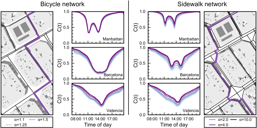
Figure 6: Network geometry can have an impact on CoolWalkability. Considering bicycle networks versus sidewalk networks can lead to different results, as links in these networks are sometimes mapped differently in OpenStreetMap. Left map: A centerline-based mapping with directed links is used for bicycle networks in Barcelona which can inaccurately reflect the actual position of bicycle tracks or is sensitive to directionality as cyclists cannot ride on the left side of the street. Right map: The sidewalk links in the same area are undirected and mapped with more detailed geometries, some of them closer to buildings and therefore shaded, which comes with more flexibility for shaded routing when walking. Middle: Accordingly, the diurnal profiles in the bicycle and sidewalk networks can differ substantially, especially for high sun avoidance $\alpha$: Sidewalk networks generally display higher CoolWalkability and are more likely to have two dips.

Network geometry matters

By “network geometry” we understand the spatial geometry used to represent the physical position of elements in a transport network. To which extent this geometry is an accurate reflection of reality depends on many factors and choices, such as the data model, data resolution, or mapping practices, which all can depend on the use case (like routing) and on the mode of transport [38, 39, 43].

In our data source OpenStreetMap, and many other map datasets, the mapped geometry that represents a street is the street’s centerline [38]. Although cyclists and pedestrians usually do not get space allocated on the centerline, but on the side of the street, centerlines are generally considered sufficient for deriving meaningful quantities like the length of a street segment. This proxy is usually adequate enough to enable effective research and applications on street networks, including routing for cyclists or pedestrians [7, 38]. In our specific use case, however, the centerline is not necessarily a reliable proxy, as the quantities of length in shade $l^{\raisebox{0.91003pt}{\scalebox{0.6}{\newmoon{}}}{}}_{a}$ and length in the sun $l^{\raisebox{0.0pt}{\scalebox{0.75}{\sun{}}}{}}_{a}$ on all edges $a$ can depend critically on the exact location of the geometry of each sidewalk in relation to the surrounding buildings. This dependence is especially relevant if the length of the shadows is in the order of the street width, like in Barcelona.

Solving this accuracy problem requires either to offset the location of the centerline geometries towards the sidewalks where pedestrians actually walk, or to acquire higher resolution networks which include the sidewalks as their own geometry. While the first approach would allow for more widespread application even for cities for which high-resolution sidewalk geometries are not available, this requires additional information on the width of each street which is often not available. This lack of exact geometry and width information is a known data limitation in sidewalk networks [38]. Fortunately, the OSM dataset of Manhattan, Barcelona and Valencia also contains many sidewalks as separate geometries, enabling the comparison between the simplified proxy based on the often centerline-based bicycle network and the full, high-resolution sidewalk network.

We therefore calculate the global CoolWalkability as a function of time for various values of the sun aversion $\alpha$ in all three studied cities on both these networks – bicycle and sidewalk. The resulting profiles can show substantial differences, depending on the observed cities, as shown in Fig. 6. Compared to the bicycle networks, in sidewalk networks the observed CoolWalkability increases for all cities, as the sidewalks are generally closer to the buildings, increasing the probability of one side being shaded. Thus, crossing the street often causes only a small detour while substantially increasing the distance travelled in shade, increasing the overall CoolWalkability even for small sun-aversions.

In addition to the overall increase in CoolWalkability, we observe an increased sensitivity with the sun-aversion $\alpha$. Where pedestrians on Manhattan’s bicycle network did not have many options of similar length from which to choose an optimal route given their individual preferences, the sidewalk network provides a multitude of such options due to the denser network and slight variations in geometry placement of the footpaths. Here the temporal location of the minima does not change, as the sun still aligns with the urban canyons at the same time; the dips do however become narrower since the duration for which both sides of the street are exposed at the same time decreases. If only one side is exposed, a pedestrian can often get into the shade by crossing the road and thus increasing the CoolWalkability, especially around the henge events. For Barcelona, the effect of the full pedestrian network is especially obvious as the profiles of the global CoolWalkability change qualitatively to now exhibit a similar double-well structure as Manhattan.

Depending on the observed city, a switch from the simplified, undirected bicycle network to the full sidewalk network with more accurately mapped pedestrian infrastructure can have either a small impact, as seen for Valencia, a mostly quantitative effect as in Manhattan or even cause a qualitative change in the dynamics, as demonstrated for Barcelona. The same effects apply to the spatial clustering plot (Fig. 5 vs. Fig. SI4), but without changing the main result of CoolWalkability clustering.

Discussion

This research represents a first exploration and method development towards the systematic study of shaded routing and the potential benefits that the built infrastructure can provide. We were able to analytically derive solutions for regular grids, to disentangle building height distribution from street network geometry, and we found a particular dependence of results on the network geometry, showing higher potential CoolWalkabilities for walking than for cycling networks. Below, we discuss the implications of these results, limitations, and relevance for urban planning and future research.

Although the street layout and building heights of existing cities are mostly static and only change slowly over time, our results reveal several insights which might be of relevance for achieving optimal shading in future urban development projects. More pointwise shading is of course achieved by narrower streets, taller buildings, or by adding trees or other objects that can block direct sunlight. However, as our analysis considered full paths and not just pointwise shade, it also exposed the nontrivial dependence of CoolWalkability on building height distributions: Especially the diurnal CoolWalkability phase portrait (Fig. 3B) reveals that at a given shadow fraction, more CoolWalkability can be achieved than expected for a perfect grid with constant building heights. We furthermore showed that an irregular street network can provide a qualitatively different diurnal CoolWalkability profile locally (Fig. 5), for example by avoiding “henge” events and corresponding dips, with very low shade availability.

A large-scale, systematic study of geometric factors such as street bearing entropy [46] in relation to CoolWalkability remains open, which could answer which network properties are most beneficial when seeking more shade for active travel. To better understand local contexts and the cause of temporal asymmetries, CoolWalkability could, for example, be investigated on rotated cities, for varying latitudes, or for larger study areas and a larger number of cities. Further, more realistic pedestrian routing scenarios could be considered beyond the sidewalk network perspective, such as traversing open areas [47], and to account for the potentially considerable time or risk involved in crossing a heavily trafficked street. Shade optimization is also not only a question of sun avoidance during hot seasons, because in other seasons too much shade can be undesirable – as demonstrated, for example, in a 10-year long study in Taiwan [22]. To identify the right annual balance between shade and sun provision depending on the local context, our model could easily be extended to also account for sun seeking.

In order to make the methods presented in this paper of further relevance to urban planning applications, researchers need access to data for pedestrian and cyclist routing of a much higher quality. The marginalization of active mobility like walking and cycling does not only happen on the policy level, but also on the level of data quality and completeness [43, 42, 38, 48]. Specifically, the lack of detailed, topologically correct, and spatially accurate data both on sidewalk and bicycle networks means that results on whether a given edge will be in shade or sun often come with substantial uncertainties. Similarly, differing mapping practices around intersections, a lack of common mapping and quality standards for street network data from the perspective of active mobility, and uncertainties on how network simplification can influence results warrant further work on active mobility networks [49, 50, 38, 48]. In addition to data quality issues for street network data, building height data are only locally available [51] and often follow different standards [52]. However, new GeoAI and image recognition tools are showing promise towards creating global, high-resolution data sets [53, 54, 55, 56].

Our research on the status quo has just started to scratch the surface of a much-neglected topic in urban planning [13]. Besides describing the existing situation, future research should ask how to use the know-how on CoolWalkability to effectively design better cities. How to identify the most optimal improvements to CoolWalkability within a given budget? The non-trivial impact of buildings, which both radiate heat and provide shade [18, 20], highlights that our focus on buildings and street networks is limited and part of a broader interdisciplinary puzzle [57, 16], which should be extended with further work on potential urban interventions like tree planting or installment of (solar panel) canopies [13]. We considered as a first step buildings only and not trees, due to availability issues with tree data. Buildings are moreover the largest shade-providing objects in cities, but are often ignored in the shade provision literature compared to trees [13]. Shade should ideally become a fundamental part of infrastructure planning via “shade master plans” and other policy guidelines [13, 14], and these plans should be based on evidence that research like ours can provide.

Central for defining the “optimality” of improvements should be the notion of equity [58]. Previous research has shown that urban “shade deserts” – places lacking the shade needed to reduce heat burden and protect human health outdoors – are part of the lived experience for low-income communities, and exacerbate heat-related health disparities [13]. Such marginalized communities have less access to shade and to air conditioning, and it is thus crucial to consider how shade provision can target those most in need.

Finally, despite the multidimensional benefits of better shade provision – including more vegetation or green canopies – on liveable cities, in the context of climate change, it must be stressed that these are primarily adaptation strategies and thus do not address the underlying core issue of human-caused increase of temperatures and extreme weather events [12].

Data availability

All data used for the experiments are publicly available at [59].

Code availability

The open-source Julia code repository is available at https://github.com/henrik-wolf/CoolWalks.

Author contributions

H.W. developed the code, conducted the experiments, performed the analytical derivations, and produced all data visualizations. All authors contributed to conceiving the model, the experiments, and visualizations. All authors analyzed the results, wrote and reviewed the manuscript. M.S. led the project and the writing. All authors have read and agreed to the final version of the manuscript.

Competing financial interests

The authors declare no competing interests.

References

- [1] Nieuwenhuijsen, M., Bastiaanssen, J., Sersli, S., Waygood, E. O. D. & Khreis, H. Implementing Car-Free Cities: Rationale, Requirements, Barriers and Facilitators. In Nieuwenhuijsen, M. & Khreis, H. (eds.) Integrating Human Health into Urban and Transport Planning, 199–219 (Springer International Publishing, Cham, 2019). URL http://link.springer.com/10.1007/978-3-319-74983-9_11.
- [2] Miner, P., Smith, B. M., Jani, A., McNeill, G. & Gathorne-Hardy, A. Car harm: A global review of automobility’s harm to people and the environment. Journal of Transport Geography 115, 103817 (2024). URL https://linkinghub.elsevier.com/retrieve/pii/S0966692324000267.
- [3] World Health Organization. Regional Office for Europe. Walking and cycling: latest evidence to support policy-making and practice (World Health Organization. Regional Office for Europe, 2022). URL https://apps.who.int/iris/handle/10665/354589.
- [4] Nieuwenhuijsen, M. et al. The Superblock model: A review of an innovative urban model for sustainability, liveability, health and well-being. Environmental Research 251, 118550 (2024). URL https://linkinghub.elsevier.com/retrieve/pii/S0013935124004547.
- [5] Szell, M., Mimar, S., Perlman, T., Ghoshal, G. & Sinatra, R. Growing urban bicycle networks. Scientific Reports 12, 6765 (2022). URL https://www.nature.com/articles/s41598-022-10783-y. Number: 1 Publisher: Nature Publishing Group.
- [6] Brand, C. et al. The climate change mitigation effects of daily active travel in cities. Transportation Research Part D: Transport and Environment 93, 102764 (2021). URL https://linkinghub.elsevier.com/retrieve/pii/S1361920921000687.
- [7] Steinacker, C., Storch, D.-M., Timme, M. & Schröder, M. Demand-driven design of bicycle infrastructure networks for improved urban bikeability. Nature Computational Science 2, 655–664 (2022).
- [8] Aldred, R., Goodman, A. & Woodcock, J. Impacts of active travel interventions on travel behaviour and health: Results from a five-year longitudinal travel survey in Outer London. Journal of Transport & Health 35, 101771 (2024).
- [9] Lovelace, R. et al. The Propensity to Cycle Tool: An open source online system for sustainable transport planning. Journal of Transport and Land Use 10 (2017).
- [10] Lenton, T. M. et al. Quantifying the human cost of global warming. Nature Sustainability 6, 1237–1247 (2023). URL https://www.nature.com/articles/s41893-023-01132-6.
- [11] Rosenzweig, C. et al. The Future We Don’t Want: How Climate Change Could Impact the World’s Greatest Cities. C40 Cities Secretariat: London, UK (2018).
- [12] Intergovernmental Panel on Climate Change. Climate Change 2022. Mitigation of Climate Change. Tech. Rep. (2022). URL https://www.ipcc.ch/report/ar6/wg3/.
- [13] Turner, V. K., Middel, A. & Vanos, J. K. Shade is an essential solution for hotter cities. Nature 619, 694–697 (2023). URL https://www.nature.com/articles/d41586-023-02311-3. Bandiera_abtest: a Cg_type: Comment Publisher: Nature Publishing Group Subject_term: Environmental sciences, Policy, Climate change.
- [14] Litman, T. Cool walkability planning: Providing pedestrian thermal comfort in hot climate cities. Journal of Civil Engineering and Environmental Sciences 9, 079–086 (2023). URL https://www.peertechzpublications.org/articles/JCEES-9-173.php.
- [15] Buehler, R. & Dill, J. Bikeway Networks: A Review of Effects on Cycling. Transport Reviews 36, 9–27 (2016). URL https://doi.org/10.1080/01441647.2015.1069908. Publisher: Routledge _eprint: https://doi.org/10.1080/01441647.2015.1069908.
- [16] Koszowski, C. et al. Active mobility: bringing together transport planning, urban planning, and public health. Towards user-centric transport in europe: challenges, solutions and collaborations 149–171 (2019).
- [17] Greenwood, J., Soulos, G. & Thomas, N. Under cover: Guidelines for shade planning and design (Cancer Society of New Zealand, 2000).
- [18] Rizwan, A. M., Dennis, L. Y. & Liu, C. A review on the generation, determination and mitigation of Urban Heat Island. Journal of Environmental Sciences 20, 120–128 (2008). URL https://linkinghub.elsevier.com/retrieve/pii/S1001074208600194.
- [19] Krayenhoff, E. S. et al. Cooling hot cities: a systematic and critical review of the numerical modelling literature. Environmental Research Letters 16, 053007 (2021). URL https://iopscience.iop.org/article/10.1088/1748-9326/abdcf1.
- [20] Li, Y., Schubert, S., Kropp, J. P. & Rybski, D. On the influence of density and morphology on the Urban Heat Island intensity. Nature Communications 11, 2647 (2020). URL https://www.nature.com/articles/s41467-020-16461-9.
- [21] Heaviside, C., Macintyre, H. & Vardoulakis, S. The Urban Heat Island: Implications for Health in a Changing Environment. Current Environmental Health Reports 4, 296–305 (2017). URL http://link.springer.com/10.1007/s40572-017-0150-3.
- [22] Lin, T.-P., Matzarakis, A. & Hwang, R.-L. Shading effect on long-term outdoor thermal comfort. Building and Environment 45, 213–221 (2010). URL https://www.sciencedirect.com/science/article/pii/S0360132309001371.
- [23] Klok, L., Rood, N., Kluck, J. & Kleerekoper, L. Assessment of thermally comfortable urban spaces in Amsterdam during hot summer days. International Journal of Biometeorology 63, 129–141 (2019).
- [24] Middel, A., AlKhaled, S., Schneider, F. A., Hagen, B. & Coseo, P. 50 Grades of Shade. Bulletin of the American Meteorological Society 102, E1805–E1820 (2021).
- [25] Olaverri Monreal, C., Pichler, M., Krizek, G. & Naumann, S. Shadow as Route Quality Parameter in a Pedestrian-Tailored Mobile Application. IEEE Intelligent Transportation Systems Magazine 8, 15–27 (2016). URL http://ieeexplore.ieee.org/document/7637096/.
- [26] Rußig, J. & Bruns, J. Reducing Individual Heat Stress through Path Planning. GI_Forum 1, 327–340 (2017). URL http://hw.oeaw.ac.at?arp=0x00369db1.
- [27] Deilami, K. et al. Allowing Users to Benefit from Tree Shading: Using a Smartphone App to Allow Adaptive Route Planning during Extreme Heat. Forests 11, 998 (2020). URL https://www.mdpi.com/1999-4907/11/9/998.
- [28] Klanjčić, M., Gauvin, L., Tizzoni, M. & Szell, M. Identifying urban features for vulnerable road user safety in Europe. EPJ Data Science 11, 1–15 (2022). URL https://epjdatascience.springeropen.com/articles/10.1140/epjds/s13688-022-00339-5. Number: 1 Publisher: SpringerOpen.
- [29] Basu, N., Oviedo-Trespalacios, O., King, M., Kamruzzaman, M. & Haque, M. M. What do pedestrians consider when choosing a route? The role of safety, security, and attractiveness perceptions and the built environment during day and night walking. Cities 143, 104551 (2023). URL https://www.sciencedirect.com/science/article/pii/S0264275123003633.
- [30] Basu, N., Haque, M. M., King, M., Kamruzzaman, M. & Oviedo-Trespalacios, O. A systematic review of the factors associated with pedestrian route choice. Transport Reviews 42, 672–694 (2022). URL https://www.tandfonline.com/doi/full/10.1080/01441647.2021.2000064.
- [31] Quercia, D., Schifanella, R. & Aiello, L. M. The shortest path to happiness: Recommending beautiful, quiet, and happy routes in the city. In Proceedings of the 25th ACM Conference on Hypertext and Social Media, HT ’14, 116–125 (Association for Computing Machinery, New York, NY, USA, 2014).
- [32] Quercia, D., Schifanella, R., Aiello, L. M. & McLean, K. Smelly Maps: The Digital Life of Urban Smellscapes. Proceedings of the International AAAI Conference on Web and Social Media 9, 327–336 (2021). URL https://ojs.aaai.org/index.php/ICWSM/article/view/14621.
- [33] Tong, Y. & Bode, N. W. F. The principles of pedestrian route choice. Journal of The Royal Society Interface 19, 20220061 (2022). URL https://royalsocietypublishing.org/doi/10.1098/rsif.2022.0061.
- [34] Dijkstra, E. W. A note on two problems in connexion with graphs. Numerische mathematik 1, 269–271 (1959).
- [35] OpenStreetMap contributors. OpenStreetMap (2023).
- [36] Building Footprints of new york. https://data.cityofnewyork.us/Housing-Development/Building-Footprints/nqwf-w8eh.
- [37] Services INSPIRE of Cadastral Cartography. http://www.catastro.minhap.gob.es/webinspire/index_eng.html.
- [38] Rhoads, D. et al. Sidewalk networks: Review and outlook. Computers, Environment and Urban Systems 106, 102031 (2023). URL https://www.sciencedirect.com/science/article/pii/S0198971523000947.
- [39] Haklay, M. M., Basiouka, S., Antoniou, V. & Ather, A. How Many Volunteers Does it Take to Map an Area Well? The Validity of Linus’ Law to Volunteered Geographic Information. The Cartographic Journal 47, 315–322 (2010).
- [40] Neis, P., Zielstra, D. & Zipf, A. The Street Network Evolution of Crowdsourced Maps: OpenStreetMap in Germany 2007–2011. Future Internet 4, 1–21 (2012). URL https://www.mdpi.com/1999-5903/4/1/1. Number: 1 Publisher: Molecular Diversity Preservation International.
- [41] Neis, P., Zielstra, D. & Zipf, A. Comparison of Volunteered Geographic Information Data Contributions and Community Development for Selected World Regions. Future Internet 5, 282–300 (2013). URL https://www.mdpi.com/1999-5903/5/2/282. Number: 2 Publisher: Multidisciplinary Digital Publishing Institute.
- [42] Ferster, C., Fischer, J., Manaugh, K., Nelson, T. & Winters, M. Using openstreetmap to inventory bicycle infrastructure: A comparison with open data from cities. International journal of sustainable transportation 14, 64–73 (2020).
- [43] Vierø, A. R., Vybornova, A. & Szell, M. How Good Is Open Bicycle Network Data? A Countrywide Case Study of Denmark. Geographical Analysis gean.12400 (2024). URL https://onlinelibrary.wiley.com/doi/10.1111/gean.12400.
- [44] Barrington-Leigh, C. & Millard-Ball, A. The world’s user-generated road map is more than 80% complete. PLOS ONE 12, e0180698 (2017).
- [45] Barthelemy, M. Spatial Networks: A Complete Introduction: From Graph Theory and Statistical Physics to Real-World Applications (Springer International Publishing, Cham, 2022). URL https://link.springer.com/10.1007/978-3-030-94106-2.
- [46] Boeing, G. Urban spatial order: Street network orientation, configuration, and entropy. Applied Network Science 4, 67 (2019).
- [47] Andreev, S., Dibbelt, J., Nöllenburg, M., Pajor, T. & Wagner, D. Towards Realistic Pedestrian Route Planning 15 pages, 1975501 bytes (2015). URL https://drops.dagstuhl.de/entities/document/10.4230/OASIcs.ATMOS.2015.1. Artwork Size: 15 pages, 1975501 bytes ISBN: 9783939897996 Medium: application/pdf Publisher: [object Object].
- [48] Zielstra, D. & Hochmair, H. H. Using Free and Proprietary Data to Compare Shortest-Path Lengths for Effective Pedestrian Routing in Street Networks. Transportation Research Record: Journal of the Transportation Research Board 2299, 41–47 (2012). URL http://journals.sagepub.com/doi/10.3141/2299-05.
- [49] Boeing, G. Osmnx: New methods for acquiring, constructing, analyzing, and visualizing complex street networks. Computers, environment and urban systems 65, 126–139 (2017).
- [50] Pung, J., D’Souza, R. M., Ghosal, D. & Zhang, M. A road network simplification algorithm that preserves topological properties. Applied Network Science 7, 79 (2022).
- [51] Biljecki, F., Chow, Y. S. & Lee, K. Quality of crowdsourced geospatial building information: A global assessment of OpenStreetMap attributes. Building and Environment 237, 110295 (2023).
- [52] Milojevic-Dupont, N. et al. EUBUCCO v0.1: European building stock characteristics in a common and open database for 200+ million individual buildings. Scientific Data 10, 147 (2023).
- [53] Biljecki, F., Stoter, J., Ledoux, H., Zlatanova, S. & Çöltekin, A. Applications of 3d city models: State of the art review. ISPRS International Journal of Geo-Information 4, 2842–2889 (2015).
- [54] Biljecki, F. & Ito, K. Street view imagery in urban analytics and gis: A review. Landscape and Urban Planning 215, 104217 (2021).
- [55] Hamim, O. F., Kancharla, S. R. & Ukkusuri, S. V. Mapping sidewalks on a neighborhood scale from street view images. Environment and Planning B: Urban Analytics and City Science 23998083231200445 (2023).
- [56] Treccani, D., Fernández, A., Díaz-Vilariño, L. & Adami, A. Automating the inventory of the navigable space for pedestrians on historical sites: towards accurate path planning. International Journal of Applied Earth Observation and Geoinformation 122, 103400 (2023).
- [57] Basagaña, X. Heat Islands/Temperature in Cities: Urban and Transport Planning Determinants and Health in Cities. In Nieuwenhuijsen, M. & Khreis, H. (eds.) Integrating Human Health into Urban and Transport Planning, 483–497 (Springer International Publishing, Cham, 2019). URL http://link.springer.com/10.1007/978-3-319-74983-9_23.
- [58] Pereira, R. H., Schwanen, T. & Banister, D. Distributive justice and equity in transportation. Transport reviews 37, 170–191 (2017).
- [59] Wolf, H. CoolWalks: Assessing the potential of shaded routing for active mobility in urban street networks - Dataset (2024). URL https://doi.org/10.5281/zenodo.11103149.