CromSS:
Cross-modal pre-training with noisy labels
for remote sensing image segmentation

Abstract

We study the potential of noisy labels $y$ to pretrain semantic segmentation models in a multi-modal learning framework for geospatial applications. Specifically, we propose a novel Cross-modal Sample Selection method (CromSS) that utilizes the class distributions $P^{(d)}(x,c)$ over pixels $x$ and classes $c$ modelled by multiple sensors/modalities $d$ of a given geospatial scene. Consistency of predictions across sensors $d$ is jointly informed by the entropy of $P^{(d)}(x,c)$. Noisy label sampling we determine by the confidence of each sensor $d$ in the noisy class label, $P^{(d)}(x,c=y(x))$.
To verify the performance of our approach, we conduct experiments with Sentinel-1 (radar) and Sentinel-2 (optical) satellite imagery from the globally-sampled SSL4EO-S12 dataset. We pair those scenes with 9-class noisy labels sourced from the Google Dynamic World project for pretraining. Transfer learning evaluations (downstream task) on the DFC2020 dataset confirm the effectiveness of the proposed method for remote sensing image segmentation.

1 Introduction

In the realm of Big Geospatial Data, one critical challenge is the lack of labeled data for deep learning model training. Self-Supervised Learning (SSL) received significant attention for its ability to extract representative features from unlabeled data (Wang et al., 2022). Popular SSL algorithms include generative Masked Autoencoders (MAE) (He et al., 2022) and contrastive learning methods such as DINO (Caron et al., 2021) and MoCo (Chen et al., 2020). MAE is inspired by image reconstruction, as most works utilizing vision transformers (ViTs) (Dosovitskiy et al., 2021). Constrastive learning methods can make a difference for both, convolutional backbones and ViTs.

Recent studies suggest that deep learning models exhibit a degree of robustness against label noise (Zhang et al., 2021; Liu et al., 2024). Promising results were observed in pretraining models with extensive volumes of noisy social-media labels for image classification (Mahajan et al., 2018) and video analysis (Ghadiyaram et al., 2019). In the realm of remote sensing (RS), pretraining on crowd-sourced maps such as OpenStreetMap for building and road extraction has been surveyed (Kaiser et al., 2017; Maggiori et al., 2017). These results indicate that inherently noisy labels can significantly reduce the level of human supervision required to effectively train deep learning models.

Moreover, as the number of launched satellites grows, we are increasingly exposed to a variety of satellite data types, including but not limited to multi-spectral, Light Detection And Ranging (LiDAR), and Synthetic Aperture Radar (SAR) data. Multi-modal learning has emerged as a prominent area of study, where the complementary information showcases efficacy in boosting the learning from different modalities, such as optical and LiDAR data (Xie et al., 2023), multi-spectral and SAR data (Chen & Bruzzone, 2022). However, the application of multi-modal learning to improve learning from noisy labels remains for detailed exploration.

In this work, we study the potential of noisy labels in multi-modal pretraining settings for RS image segmentation, where a novel Cross-modal Sample Selection method, referred to as CromSS, is introduced to further mitigate the adverse impact of label noise. In the pretraining stage, we first employ two U-Nets (Ronneberger et al., 2015) backboned with ResNet-50 (He et al., 2016) to separately extract features and generate confidence masks within each modality. After that, the sample selection is implemented for each modality on its enhanced confidence masks by fortifying the shared information across modalities. Given that radar and optical satellites are sensitive to distinct features on the ground, such cross-modal enhancement bears potential to boost the mutual learning between modalities. We test middle and late fusion strategies to improve the architecture design for multi-modal learning. In our experiments, we utilize Sentinel-1 (S1) of radar and Sentinel-2 (S2) of multi-spectral data from the SSL4EO-S12 dataset (Wang et al., 2023) as two modalities. We pair those scenes with pixel-wise noisy labels of the Google Dynamic World (DW) project (Brown et al., 2022) for pretraining. Evaluation of the pretrained ResNet-50 encoders is based on the DFC2020 dataset (Yokoya, 2019) referenced to pretrained DINO and MoCo models presented as baselines in the SSL4EO-S12 work.

2 Data

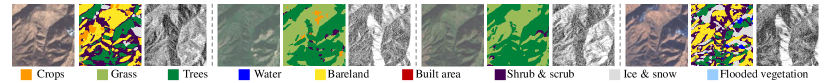
Figure 1: An example of sentinel-1 (VV, right) and sentinel-2 (RGB, left) data paired with noisy labels (middle) from 4 seasons.

In the pretraining stage, we utilize the extended version of the SSL4EO-S12 dataset, a large-scale self-supervision dataset in Earth observation, plus 9-class noisy labels sourced from the DW project on the Google Earth Engine as illustrated in Figure 1. SSL4EO-S12 sampled data globally from 251,079 locations. Each location corresponds to 4 S1 and S2 image pairs of 264$\times$264 pixels from 4 different seasons, among which 103,793 locations have noisy label masks matched for all the seasons. We only utilize the image-label pairs of these 103,793 locations for pretraining with noisy labels.

Notice that this dataset is a good reflection of real cases, where noisy labels are still harder to obtain compared to images, thus of a smaller size than unlabeled data. We utilize DFC2020 as the downstream segmentation task, where the 986 validation patches are used as the fine-tuning training data with the 5128 test ones for test.

3 Methodology

Our methodology links semantic segmentation maps of single-modal models by two principles: (a) consistent prediction of the physical ground truth (consistency loss $L_{c}$), and (b) tolerance to noisy supervision (segmentation loss $L_{s}$). For the latter, we extend the idea of Cao & Huang (2022) working on a single modality to multiple modalities with cross-modal interactions for estimating the uncertainty of a given pixel-level class label. Each modality-specific model predicts the probability $P^{(d)}$ of a given noisy label at a physical location. While one model $d=1$ may be certain about the label $y$, another $d=2$ may assign low probability: $P^{(1)}(y)\gg P^{(2)}(y)$. Section 3.2 details on how we integrate these information to obtain a cross-modality score of a label perceived noisy. Similarly, we exploit the entropy of $P^{(d)}$ to introduced a criterion for a cross-modality consistency loss on label predictions between single-modality models. The overall approach is summarized by Figure 2, where $Q^{(d)}$ represents an estimate of $P^{(d)}$.

3.1 Multi-modal fusion

We employ middle and late multi-modal fusion (Chen & Bruzzone, 2022) to explore the complementary information across modalities to aid model training. Our fusion strategies do not concatenate feature vectors of different modalities. While middle fusion shares a common decoder for all modalities, late fusion retains individual decoders.

3.2 Cross-modal sample selection

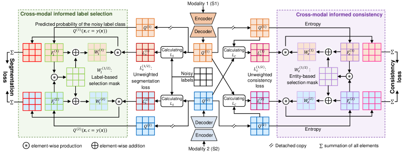
Figure 2: Illustration of the proposed CromSS. The decoders in the middle share the weights when middle fusion is applied. In late fusion, they are separately optimized per modality. The shaded areas (green to the left, purple to the right) highlight the key components of cross-modal sample selection.

As depicted by Figure 2, the key in CromSS when compared to naive multi-modal training is the introduction of sample selection masks $\mathbf{\mathcal{missing}}{W}_{l/e}^{(d)}$ (the shaded areas in Figure 2). They serve as weights for calculating the segmentation and consistency losses, $L_{s}$ and $L_{c}$, cf. the label-based masks $\mathbf{\mathcal{missing}}{W}_{l}^{(d)}$ and the entity-based masks $\mathbf{\mathcal{missing}}{W}_{e}^{(d)}$ for modality $d$.

To compute $\mathbf{\mathcal{missing}}{W}_{l}^{(d)}$ and $\mathbf{\mathcal{missing}}{W}_{e}^{(d)}$, we first generate the corresponding confidence masks $\mathbf{\mathcal{missing}}{F}_{l}^{(d)}$ and $\mathbf{\mathcal{missing}}{F}_{e}^{(d)}$ from the softmax outputs, i.e., the estimated class distributions $Q^{(d)}$ for $P^{(d)}$. Let $q_{i,j,c}^{(d)}\in Q^{(d)}$ denote the softmax output at image pixel location $(i,j)$ and class $c$, and $y_{i,j}$ be its given noisy label. Then, we take $q_{i,j,c}^{(d)}$ with $c=y_{i,j}$ as the estimated label-based confidence scores in $\mathbf{\mathcal{missing}}{F}_{l}^{(d)}$. For the entity-based confidence, we define $f_{(e)i,j}^{(d)}\in\mathbf{\mathcal{missing}}{F}_{e}^{(d)}$ using the entropy of its softmax vector $h_{i,j}^{(d)}$ as follows,

$${f_{(e)i,j}^{(d)}=1-{h_{i,j}^{(d)}}/{K}=1+\tfrac{1}{K}\sum_{c=1}^{C}q_{i,j,c}^{(d)}\log q_{i,j,c}^{(d)}}$$ (1)

where $C$ is the total number of classes, $K=\log C$ is the upper bound of $h_{i,j}\in[0,K]$ when $q_{i,j,c}=1/C$ for $c=1,\cdots,C$, i.e., equal distribution of maximum entropy. For two modalities $d\in\{1,2\}$, the final confidence masks are combined into the following:

$$\mathbf{\mathcal{missing}}{F^{\prime}}_{l/e}^{(1/2)}={\tfrac{1}{2}\left(\mathbf{\mathcal{missing}}{F}_{l/e}^{(1/2)}+\mathbf{\mathcal{missing}}{F}_{l/e}^{(1)}\mathbf{\mathcal{missing}}{F}_{l/e}^{(2)}\right)}=\tfrac{1}{2}\mathbf{\mathcal{missing}}{F}_{l/e}^{(1/2)}\left(1+\mathbf{\mathcal{missing}}{F}_{l/e}^{(2/1)}\right)\quad,$$ (2)

where the factor $\mathbf{\mathcal{missing}}{F}_{l/e}^{(1/2)}\mathbf{\mathcal{missing}}{F}_{l/e}^{(2/1)}$ serves to magnify the selection probabilities of the samples exhibiting high confidence while diminishing cases where both modalities $d=1$ and $d=2$ agree on low confidence score. To generate final sample selection masks, we utilize a soft selection strategy rather than the one-hot selection masks for $\mathbf{\mathcal{missing}}{W}_{l}^{(d)}$, in order to avoid models from enforcing their own prediction errors. Mathematically speaking: given the selection ratio $\alpha\in[0,1]$, we define ${w}_{i,j}^{(d)}\in\mathbf{\mathcal{missing}}{W}_{l}^{(d)}$ as,

$$\mathbf{\mathcal{missing}}{w}_{i,j}^{(d)}=\min\left[1,{{f^{\prime}}^{(d)}_{i,j}}/w\right]\quad,$$ (3)

where ${f^{\prime}}^{(d)}_{i,j}\in\mathbf{\mathcal{missing}}{F^{\prime}}_{l}^{(d)}$, $w$ is the $(\alpha\cdot n)$th highest value in $\mathbf{\mathcal{missing}}{F^{\prime}}_{l}^{(d)}$ with $n$ denoting the size of $\mathbf{\mathcal{missing}}{F^{\prime}}_{l}^{(d)}$. For the consistency loss, we utilize the weighting factor $\gamma\in[0,1]$ to generate $W_{e}^{(d)}$ from $\mathbf{\mathcal{missing}}{F^{\prime}}_{e}^{(d)}$ as $W_{e}^{(d)}=(1-\gamma)+\gamma\mathbf{\mathcal{missing}}{F^{\prime}}_{e}^{(d)}$ with $\gamma$ gradually ramping up from 0 to 1 during the training. With the losses weighted by $\mathbf{\mathcal{missing}}{W}_{l}^{(d)}$ and $\mathbf{\mathcal{missing}}{W}_{e}^{(d)}$, the samples of lower confidence can contribute less in the optimization process.

4 Experiments

We pretrained ResNet-50 (He et al., 2016) nested in U-Nets (Ronneberger et al., 2015) using the combined segmentation losses of CrossEntropy and Dice (Jadon, 2020) along with Kullback-Leibler divergence (Kullback & Leibler, 1951) serving as the consistency losses. The selection proportion $\alpha$ we set to 50% after exponentially ramping down from 100% for the first 80 epochs. At the same time, the weighting factor $\gamma$ ramps up from 0 to 1 in parallel. We employed a seasonal data augmentation strategy, where the data from a randomly selected season were fed to U-Nets in each iteration. An Adam optimizer (Kingma & Ba, 2017) was used with a learning rate of $.5\cdot 10^{-3}$. We employed the ReduceLROnPlateau scheduler to cut in half the learning rate when the validation loss is not decreasing over 30 consecutive epochs. We randomly split off 1% of the entire training set as the validation set. The pretraining was implemented on 4 NVIDIA A100 GPUs running approx. 13 hours for 100 epochs. When transferred to the DFC2020 dataset, pretrained ResNet-50 encoders were embedded into PSPNets (Zhao et al., 2017), fine-tuned with Adam and a learning rate of $.5\cdot 10^{-4}$ for 50 epochs. As reference, we also present the results of single-modal pretraining (S1/S2) as well as multi-modal pretraining without sample selection, in which midF and lateF denote middle and late fusion, respectively. Pretrained weights by DINO and MoCo were provided by Wang et al. (2023). Results reported with error bars stem from 3 repeated runs of each setup.

Table 1: Transfer learning results on the DFC2020 dataset with S1 and S2 as inputs, respectively, where “Fine-tuned” and “Frozen” indicate whether the encoder weights would be adjusted along with decoder ones or not.

Modality	Encoder	Frozen			Fine-tuned
	Metrics	OA	AA	mIoU	OA	AA	mIoU
S1	Random	54.41$\pm$0.35	40.68$\pm$0.23	29.16$\pm$0.06	52.65$\pm$0.42	42.17$\pm$0.29	28.36$\pm$0.22
	MoCo	60.88$\pm$0.41	47.46$\pm$0.52	34.25$\pm$0.27	60.31$\pm$0.40	44.98$\pm$0.66	31.80$\pm$0.46
	single-modal (S1)	61.73$\pm$0.58	46.13$\pm$0.34	34.77$\pm$0.30	61.07$\pm$0.19	45.78$\pm$0.48	34.13$\pm$0.19
	midF	62.08$\pm$0.73	45.01$\pm$0.40	34.64$\pm$0.48	61.24$\pm$0.44	45.44$\pm$0.84	33.86$\pm$0.16
	lateF	61.09$\pm$0.11	45.77$\pm$0.29	34.15$\pm$0.14	62.19$\pm$0.49	47.43$\pm$0.41	34.58$\pm$0.48
	CromSS-midF	61.66$\pm$0.41	45.07$\pm$0.28	34.38$\pm$0.02	62.32$\pm$1.01	47.19$\pm$0.84	35.17$\pm$0.63
	CromSS-lateF	62.58$\pm$0.36	46.37$\pm$0.53	34.80$\pm$0.37	60.92$\pm$0.76	46.13$\pm$0.60	33.94$\pm$0.55
S2	random	56.42$\pm$0.49	45.12$\pm$0.18	31.50$\pm$0.14	58.68$\pm$0.77	46.03$\pm$0.43	33.56$\pm$0.28
	DINO	64.82$\pm$0.22	48.83$\pm$0.08	37.81$\pm$0.08	63.64$\pm$0.72	49.92$\pm$1.33	36.95$\pm$0.55
	MoCo	63.25$\pm$0.47	51.00$\pm$0.28	37.67$\pm$0.57	61.19$\pm$0.39	47.29$\pm$0.36	34.86$\pm$0.63
	single-modal (S2)	66.66$\pm$0.19	53.24$\pm$0.21	40.88$\pm$0.07	67.11$\pm$0.22	53.14$\pm$0.69	41.06$\pm$0.24
	midF	68.36$\pm$0.65	53.23$\pm$0.42	41.52$\pm$0.35	68.07$\pm$0.64	52.60$\pm$0.52	41.17$\pm$0.28
	lateF	67.61$\pm$0.91	54.08$\pm$0.92	41.59$\pm$0.75	68.43$\pm$1.18	53.72$\pm$0.76	41.76$\pm$0.76
	CromSS-midF	69.41$\pm$0.68	55.97$\pm$0.31	42.89$\pm$0.35	69.20$\pm$0.66	54.86$\pm$0.59	42.58$\pm$0.34
	CromSS-lateF	66.61$\pm$1.20	54.23$\pm$1.06	41.12$\pm$0.11	69.10$\pm$0.29	54.86$\pm$0.42	42.55$\pm$0.36

As shown in Table 1, the proposed CromSS can improve the effectiveness of the pretrained encoders in remote sensing image segmentation—in particular for S2 multi-spectral data. The improvement for S1 radar data is less significant. We attribute this discrepancy to the different capabilities of two modalities in the pretraining task, i.e., land cover classification in this work. The sample selection in CromSS is still fundamentally based on its own confidence masks for each modality. S1, which can be regarded as a weak modality in this case, can potentially take more advantages from S2 with additional specific strategies. Furthermore, the middle fusion strategy showcases a larger margin compared to late fusion, which indicates that the implicit data fusion via decoder weight sharing can boost the learning across modalities to some extent. We can also observe some improvements of single-modal pretraining with noisy labels compared to DINO and MoCo. These outcomes further demonstrate the potential of using noisy labels in task-specific pretraining for segmentation downstream tasks.

5 Conclusions

With CromSS we introduce a pretraining strategy guided by noisy labels for large-scale remote sensing image segmentation. CromSS exploits a cross-modal sample selection strategy to reduce the adverse effects of label noise. We combine this approach with a consistency loss correlating models each of which operates on a single modality, only. Transfer learning results on the DFC2020 dataset demonstrate the effectiveness of the CromSS-pretrained ResNet-50 encoders. In future works, we will explore the potential of CromSS for ViT pretraining such as in Masked-Image-Modelling as well as on more kinds of noisy labels to test its robustness to different noise rates.

Acknowledgments

The work of C. Liu, Y. Wang and C. Albrecht was funded by the Helmholtz Association through the Framework of HelmholtzAI, grant ID: ZT-I-PF-5-01 – Local Unit Munich Unit @Aeronautics, Space and Transport (MASTr). The compute related to this work was supported by the Helmholtz Association’s Initiative and Networking Fund on the HAICORE@FZJ partition. C. Albrecht receives additional funding from the European Union’s Horizon Europe research and innovation programme under grant agreement No. 101082130 (EvoLand). The work of X. X. Zhu is jointly supported by the Excellence Strategy of the Federal Government and the Länder through the TUM Innovation Network EarthCare, by the German Federal Ministry of Education and Research (BMBF) in the framework of the international future AI lab “AI4EO – Artificial Intelligence for Earth Observation: Reasoning, Uncertainties, Ethics and Beyond” (grant number: 01DD20001) and by Munich Center for Machine Learning.

References

- Brown et al. (2022) Christopher F. Brown, Steven P. Brumby, Brookie Guzder-Williams, Tanya Birch, Samantha Brooks Hyde, Joseph Mazzariello, Wanda Czerwinski, Valerie J. Pasquarella, Robert Haertel, Simon Ilyushchenko, Kurt Schwehr, Mikaela Weisse, Fred Stolle, Craig Hanson, Oliver Guinan, Rebecca Moore, and Alexander M. Tait. Dynamic World, Near real-time global 10 m land use land cover mapping. Scientific Data, 9(1):251, June 2022. ISSN 2052-4463. doi: 10.1038/s41597-022-01307-4. URL https://www.nature.com/articles/s41597-022-01307-4. Number: 1.
- Cao & Huang (2022) Yinxia Cao and Xin Huang. A coarse-to-fine weakly supervised learning method for green plastic cover segmentation using high-resolution remote sensing images. ISPRS Journal of Photogrammetry and Remote Sensing, 188:157–176, June 2022. ISSN 0924-2716. doi: 10.1016/j.isprsjprs.2022.04.012. URL https://www.sciencedirect.com/science/article/pii/S0924271622001095.
- Caron et al. (2021) Mathilde Caron, Hugo Touvron, Ishan Misra, Hervé Jégou, Julien Mairal, Piotr Bojanowski, and Armand Joulin. Emerging Properties in Self-Supervised Vision Transformers. pp. 9650–9660, 2021. URL https://openaccess.thecvf.com/content/ICCV2021/html/Caron_Emerging_Properties_in_Self-Supervised_Vision_Transformers_ICCV_2021_paper.html.
- Chen et al. (2020) Xinlei Chen, Haoqi Fan, Ross Girshick, and Kaiming He. Improved Baselines with Momentum Contrastive Learning, March 2020. URL http://arxiv.org/abs/2003.04297. arXiv:2003.04297 [cs].
- Chen & Bruzzone (2022) Yuxing Chen and Lorenzo Bruzzone. Self-Supervised SAR-Optical Data Fusion of Sentinel-1/-2 Images. IEEE Transactions on Geoscience and Remote Sensing, 60:1–11, 2022. ISSN 1558-0644. doi: 10.1109/TGRS.2021.3128072. URL https://ieeexplore.ieee.org/document/9614157. Conference Name: IEEE Transactions on Geoscience and Remote Sensing.
- Dosovitskiy et al. (2021) Alexey Dosovitskiy, Lucas Beyer, Alexander Kolesnikov, Dirk Weissenborn, Xiaohua Zhai, Thomas Unterthiner, Mostafa Dehghani, Matthias Minderer, Georg Heigold, Sylvain Gelly, Jakob Uszkoreit, and Neil Houlsby. An Image is Worth 16x16 Words: Transformers for Image Recognition at Scale, June 2021. URL http://arxiv.org/abs/2010.11929. arXiv:2010.11929 [cs].
- Ghadiyaram et al. (2019) Deepti Ghadiyaram, Du Tran, and Dhruv Mahajan. Large-Scale Weakly-Supervised Pre-Training for Video Action Recognition. pp. 12046–12055, 2019. URL https://openaccess.thecvf.com/content_CVPR_2019/html/Ghadiyaram_Large-Scale_Weakly-Supervised_Pre-Training_for_Video_Action_Recognition_CVPR_2019_paper.html.
- He et al. (2016) Kaiming He, Xiangyu Zhang, Shaoqing Ren, and Jian Sun. Deep Residual Learning for Image Recognition. pp. 770–778, 2016. URL https://openaccess.thecvf.com/content_cvpr_2016/html/He_Deep_Residual_Learning_CVPR_2016_paper.html.
- He et al. (2022) Kaiming He, Xinlei Chen, Saining Xie, Yanghao Li, Piotr Dollár, and Ross Girshick. Masked Autoencoders Are Scalable Vision Learners. pp. 16000–16009, 2022. URL https://openaccess.thecvf.com/content/CVPR2022/html/He_Masked_Autoencoders_Are_Scalable_Vision_Learners_CVPR_2022_paper.
- Jadon (2020) Shruti Jadon. A survey of loss functions for semantic segmentation. In 2020 IEEE Conference on Computational Intelligence in Bioinformatics and Computational Biology (CIBCB), pp. 1–7, October 2020. doi: 10.1109/CIBCB48159.2020.9277638. URL https://ieeexplore.ieee.org/document/9277638.
- Kaiser et al. (2017) Pascal Kaiser, Jan Dirk Wegner, Aurélien Lucchi, Martin Jaggi, Thomas Hofmann, and Konrad Schindler. Learning Aerial Image Segmentation From Online Maps. IEEE Transactions on Geoscience and Remote Sensing, 55(11):6054–6068, November 2017. ISSN 1558-0644. doi: 10.1109/TGRS.2017.2719738. Number: 11.
- Kingma & Ba (2017) Diederik P. Kingma and Jimmy Ba. Adam: A Method for Stochastic Optimization, January 2017. URL http://arxiv.org/abs/1412.6980. arXiv:1412.6980 [cs].
- Kullback & Leibler (1951) S. Kullback and R. A. Leibler. On Information and Sufficiency. The Annals of Mathematical Statistics, 22(1):79–86, March 1951. ISSN 0003-4851, 2168-8990. doi: 10.1214/aoms/1177729694. URL https://projecteuclid.org/journals/annals-of-mathematical-statistics/volume-22/issue-1/On-Information-and-Sufficiency/10.1214/aoms/1177729694.full. Publisher: Institute of Mathematical Statistics.
- Liu et al. (2024) Chenying Liu, Conrad Albrecht, Yi Wang, and Xiao Xiang Zhu. Task specific pretraining with noisy labels for remote sensing image segmentation, 2024. URL https://arxiv.org/abs/2402.16164.
- Maggiori et al. (2017) Emmanuel Maggiori, Yuliya Tarabalka, Guillaume Charpiat, and Pierre Alliez. Convolutional Neural Networks for Large-Scale Remote-Sensing Image Classification. IEEE Transactions on Geoscience and Remote Sensing, 55(2):645–657, February 2017. ISSN 1558-0644. doi: 10.1109/TGRS.2016.2612821. Number: 2.
- Mahajan et al. (2018) Dhruv Mahajan, Ross Girshick, Vignesh Ramanathan, Kaiming He, Manohar Paluri, Yixuan Li, Ashwin Bharambe, and Laurens van der Maaten. Exploring the Limits of Weakly Supervised Pretraining. pp. 181–196, 2018. URL https://openaccess.thecvf.com/content_ECCV_2018/html/Dhruv_Mahajan_Exploring_the_Limits_ECCV_2018_paper.html.
- Ronneberger et al. (2015) Olaf Ronneberger, Philipp Fischer, and Thomas Brox. U-Net: Convolutional Networks for Biomedical Image Segmentation. In Nassir Navab, Joachim Hornegger, William M. Wells, and Alejandro F. Frangi (eds.), Medical Image Computing and Computer-Assisted Intervention – MICCAI 2015, Lecture Notes in Computer Science, pp. 234–241, Cham, 2015. Springer International Publishing. ISBN 978-3-319-24574-4. doi: 10.1007/978-3-319-24574-4˙28.
- Wang et al. (2022) Yi Wang, Conrad M. Albrecht, Nassim Ait Ali Braham, Lichao Mou, and Xiao Xiang Zhu. Self-Supervised Learning in Remote Sensing: A review. IEEE Geoscience and Remote Sensing Magazine, 10(4):213–247, December 2022. ISSN 2168-6831. doi: 10.1109/MGRS.2022.3198244. URL https://ieeexplore.ieee.org/document/9875399. Conference Name: IEEE Geoscience and Remote Sensing Magazine.
- Wang et al. (2023) Yi Wang, Nassim Ait Ali Braham, Zhitong Xiong, Chenying Liu, Conrad M. Albrecht, and Xiao Xiang Zhu. SSL4EO-S12: A large-scale multimodal, multitemporal dataset for self-supervised learning in Earth observation [Software and Data Sets]. IEEE Geoscience and Remote Sensing Magazine, 11(3):98–106, September 2023. ISSN 2168-6831. doi: 10.1109/MGRS.2023.3281651. URL https://ieeexplore.ieee.org/abstract/document/10261879. Conference Name: IEEE Geoscience and Remote Sensing Magazine.
- Xie et al. (2023) Yuxing Xie, Jiaojiao Tian, and Xiao Xiang Zhu. A co-learning method to utilize optical images and photogrammetric point clouds for building extraction. International Journal of Applied Earth Observation and Geoinformation, 116:103165, February 2023. ISSN 1569-8432. doi: 10.1016/j.jag.2022.103165. URL https://www.sciencedirect.com/science/article/pii/S1569843222003533.
- Yokoya (2019) Naoto Yokoya. 2020 IEEE GRSS Data Fusion Contest, December 2019. URL https://ieee-dataport.org/competitions/2020-ieee-grss-data-fusion-contest.
- Zhang et al. (2021) Chiyuan Zhang, Samy Bengio, Moritz Hardt, Benjamin Recht, and Oriol Vinyals. Understanding deep learning (still) requires rethinking generalization. Communications of the ACM, 64(3):107–115, February 2021. ISSN 0001-0782. doi: 10.1145/3446776. URL https://doi.org/10.1145/3446776. Number: 3.
- Zhao et al. (2017) Hengshuang Zhao, Jianping Shi, Xiaojuan Qi, Xiaogang Wang, and Jiaya Jia. Pyramid Scene Parsing Network. pp. 2881–2890, 2017. URL https://openaccess.thecvf.com/content_cvpr_2017/html/Zhao_Pyramid_Scene_Parsing_CVPR_2017_paper.html.