Modeling pedestrian fundamental diagram based on
Directional Statistics

Abstract

Understanding pedestrian dynamics is crucial for appropriately designing pedestrian spaces. The pedestrian fundamental diagram (FD), which describes the relationship between pedestrian flow and density within a given space, characterizes these dynamics. Pedestrian FDs are significantly influenced by the flow type, such as uni-directional, bi-directional, and crossing flows. However, to the authors’ knowledge, generalized pedestrian FDs that are applicable to various flow types have not been proposed. This may be due to the difficulty of using statistical methods to characterize the flow types. The flow types significantly depend on the angles of pedestrian movement; however, these angles cannot be processed by standard statistics due to their periodicity. In this study, we propose a comprehensive model for pedestrian FDs that can describe the pedestrian dynamics for various flow types by applying Directional Statistics. First, we develop a novel statistic describing the pedestrian flow type solely from pedestrian trajectory data using Directional Statistics. Then, we formulate a comprehensive pedestrian FD model that can be applied to various flow types by incorporating the proposed statistics into a traditional pedestrian FD model. The proposed model was validated using actual pedestrian trajectory data. The results confirmed that the model effectively represents the essential nature of pedestrian dynamics, such as the capacity reduction due to conflict of crossing flows and the capacity improvement due to the lane formation in bi-directional flows.

1 Introduction

Understanding pedestrian dynamics is essential for appropriately designing pedestrian spaces, such as corridors and public squares. Flow, density, and speed are the most basic state variables of pedestrian flow. A fundamental diagram (FD), which is the relationships between these variables, characterizes pedestrian flow and determines the important features such as the flow capacity. In addition, FDs are useful for evaluating pedestrian flow models and developing dynamic simulation models [1]. For these reasons, FDs are important and form the basis for the design of pedestrian spaces.

The specific natures of pedestrian flow should be taken into account in the modeling of the pedestrian FD, since FD was initially developed for vehicular flow. May [2] showed similarities and differences between pedestrian and vehicular flows. One of the most essential differences is that pedestrian flow is not unidirectional. Thus, pedestrians often conflict with others’ movement, and their collective behavior becomes very complicated.

The multi-directionality of pedestrian flow gives rise to complicated phenomena. Let us consider a unidirectional pedestrian flow as a reference. For example, if two pedestrian flows intersect at a 90-degree angles, capacity and speed will decrease due to potential collisions. However, if two pedestrian flows pass each other at a 180-degrees angles, capacity and speed will remain the same or even increase due to the self-organization phenomena called lane formation [3]. If pedestrian flows with various angles intersects, it is not easy to predict the resulting flow. Vanume et al. [1] reviewed that this kind of flow type of pedestrian affects pedestrian FDs in a complicated manner.

Flow types might be quantitatively distinguished by the angle of the pedestrians movement direction. The histograms in figure 1 show the distributions of the pedestrians movement direction obtained from the actual data. Uni/bi-directional flow means the flow passing through a corridor uni/bi-directionally. Crossing-A flow is defined as the flow through a crossing bi-directionally, and crossing-B flow is defined as the flow through a crossing uni-directionally. It is clear that the distribution shape of the angle is different for each flow type. Therefore, at least in qualitatively, flow types can be classified by the shape of the distribution of the angle of the pedestrians movement direction.

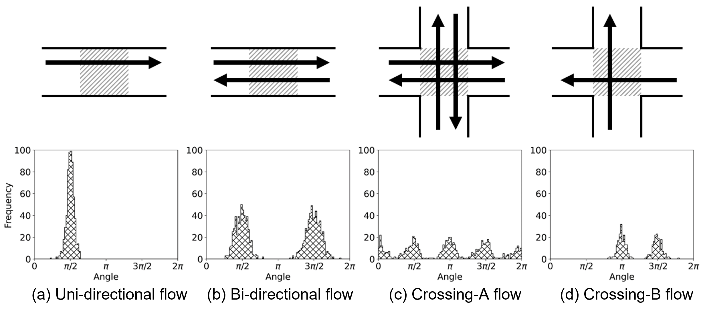
Figure 1: Four examples of flow types and their histograms. The data is a 10-second sample for each flow type from the data used in the case study.

However, angle is difficult to analyze quantitatively or statistically due to its periodicity. For example, the meaningful average of 1-degree and 359-degree angles should be 0-degree, not 180 that is the arithmetic mean of 1 and 359. This poses us significant difficulty for computing statistics of pedestrian moving direction such as the mean and variance of moving angles, which could be a useful statistics to characterize the flow type.

To tackle this challenge, this study employs Directional Statistics [4] specifically designed for analyzing angles. It has been applied to several research fields such as wind direction [5] and animal movement direction [6]. Recently, it is also applied to analyze transportation maps [7][8][9]. However, to the authors’ knowledge, its application in dynamical transportation phenomena such as pedestrian flow is unseen.

This study aims to develop a pedestrian FD model that can be applied to various flow types regardless of its configuration. The proposed model can capture the complicated pedestrian phenomena associated with flow types in a simple and straightforward manner by leveraging the Directional Statistics. To achieve this, we propose a novel statistic termed $p$th angular variance to effectively characterize pedestrian flow. The features of the proposed model is validated by applying it to actual pedestrian trajectory data.

2 Literature review

Pedestrian FDs have been studied widely in the literature. The simplest studies on pedestrian FDs are those on uni-directional flows. Based on data obtained from experiments or observations, many FD models of uni-directional flow have been proposed.

One of the earliest model is that proposed by Fruin [10]. He formulated the flow $J$ as a function of density $\rho$ in the form of an equation as

$$J=\frac{A\rho-B}{\rho^{2}},$$ (1)

where $A$ and $B$ are parameters. Virkler and Elayadath [11] applied several FD models that had been applied to vehicular flows to pedestrian flows. Seyfried et al. [12] showed from observation that a linear relationship between speed and the inverse of density can be established for single-row pedestrian flows. Furthermore, they showed that the same relationship can be applied to general uni-directional flows by comparison with literature values. Existing studies about uni-directional flows mostly modeled flow (or speed) as a function of density only.

Bi-directional flow is compared with uni-directional flow by pedestrian flow data in some studies. Zhang and Seyfried [13] showed that the flow rate of bi-directional flow is significantly lower than that of uni-directional flow at high densities. Lam et al. [14] showed that the capacity of a pedestrian space decreases in bi-directional flows. These studies showed that bi-directional flow is less efficient than uni-directional flow.

On the other hand, an efficient condition of bi-directional flow, named lane formation, has also been studied [3][15]. Jia et al. [16] proposed a parameter that represents the degree of deviation from the lane generated by lane formation and examined its correlation with the pedestrian’s egress time from the exit. The results showed that there was a positive correlation between the degree of deviation and the egress time, which suggests that the occurrence of lane formation makes the pedestrian flow more efficient. Lee et al. [17] showed the capacity is improved by occurrence of lane formation in the simulation.

Multi-directional flows other than bi-directional flows have also been observed by researchers. Zhang et al. [18] compared uni-directional and T-junction flows and found that their FDs were different. Cao et al. [19] and Zhang et al. [13] compared uni-directional, bi-directional, and crossing flows. Both studies found that the capacities of bi-directional and crossing flows were smaller than those of uni-directional flows. Iryo and Nagashima [20] showed that flows crossing angles of 45^∘ and 135^∘ tended to have lower flow than flows at 90^∘, even at the same density.

Multi-directional flows are often described using physical models. A well-known example is the social force model developed by Helbing and Molnar [21]. In this model, the pedestrian is regarded as a point mass. The motivation of the pedestrian moving to the desired direction, the influence between pedestrians, and the influence of walls are regarded as forces acting on the point mass. The forced pedestrians’ moves are based on the equations of motion. The social force model has been extended in various ways [22][23] and has been successful in terms of reproducing the pedestrian flows. Nakanishi and Fuse [24] analyzed pedestrian movements by focusing on their moving direction. They regarded pedestrian trajectories as data consisting of the pedestrian’s position and angle of moving direction at each time. A correlation between pedestrian position and direction of travel was discovered by basic analysis of pedestrian trajectories in front of ticket gates, and a regression model was constructed. However, these studies were not performed on modeling pedestrian FD.

There are few studies modeling the FDs of pedestrian flows other than uni-directional flows. Flötteröd and Lämmel [25] formulated a parametric FD for bi-directional flow based on cellular automata. Feliciani et al. [26] modeled an FD for bi-directional flow by applying the flow ratio, which is defined as the ratio of flow in one direction and flow in the other direction. However, these models cannot be applied to flow types other than bi-directional or uni-directional flow. Moustaid and Flötteröd [27] proposed an FD model for multi-directional flow by extending a macroscopic node model [28] for vehicular traffic flow. However, it requires pre-processing of pedestrian data to decompose the flow into specific number of directions. It limits the generality of the model (i.e., an estimated model is specialized for a specific location with specific node-link configuration). A model of pedestrian FDs comprehensively applicable to multiple flow types has not been developed.

3 Model

We formulate a comprehensive pedestrian FD model that can represent the effects of pedestrian avoidance of conflicts and lane formation. The proposed model is formulated by extending a simple functional form of FD using the angular variance.

Note that in the following discussion, the unit of angle is radian.

3.1 Angular variance

Angular variance [4] is a statistic that describes the degree of dispersion for angular data. The angular variance $\nu_{1}$ for $N$ angular data $\theta_{j}(j=1,2,\ldots,N)$ is defined by

$$\nu_{1}=1-\bar{R}_{1},$$ (2)

where,

$$\bar{R}_{1}=\sqrt{\bar{C}_{1}^{2}+\bar{S}_{1}^{2}},$$ (3)

$$\bar{C}_{1}=\frac{1}{N}\sum_{j=1}^{N}\cos\theta_{j},\quad\bar{S}_{1}=\frac{1}{N}\sum_{j=1}^{N}\sin\theta_{j}.$$ (4)

For the $j$th angular data $\theta_{j}$, $(\cos\theta_{j},\sin\theta_{j})^{\top}$ represents the unit vector for that angle, where ^⊤ means the transpose of vector. Therefore, $(\bar{C}_{1},\bar{S}_{1})^{\top}$ is the composite of $N$ unit vectors divided by its data size $N$. $\bar{R}_{1}$ is the norm of $(\bar{C}_{1},\bar{S}_{1})^{\top}$, which takes a value between $0$ and $1$, and it varies depending on the degree of dispersion of the data.

The definition of the angular variance ${\nu}_{1}$ is $1-\bar{R}_{1}$. The value of ${\nu}_{1}$ gets larger when the data is scattered, which is consistent with the conventional statistics.

For example, as shown in the left of Figure 2(a), when the angular data are concentrated in a close direction, $\nu_{1}$ takes a value close to 0. On the other hand, when the angular data are dispersed in opposite directions, as the example shown in the right of Figure 2(a), $\nu_{1}$ takes a value close to 1 because unit vectors cancel each other out.

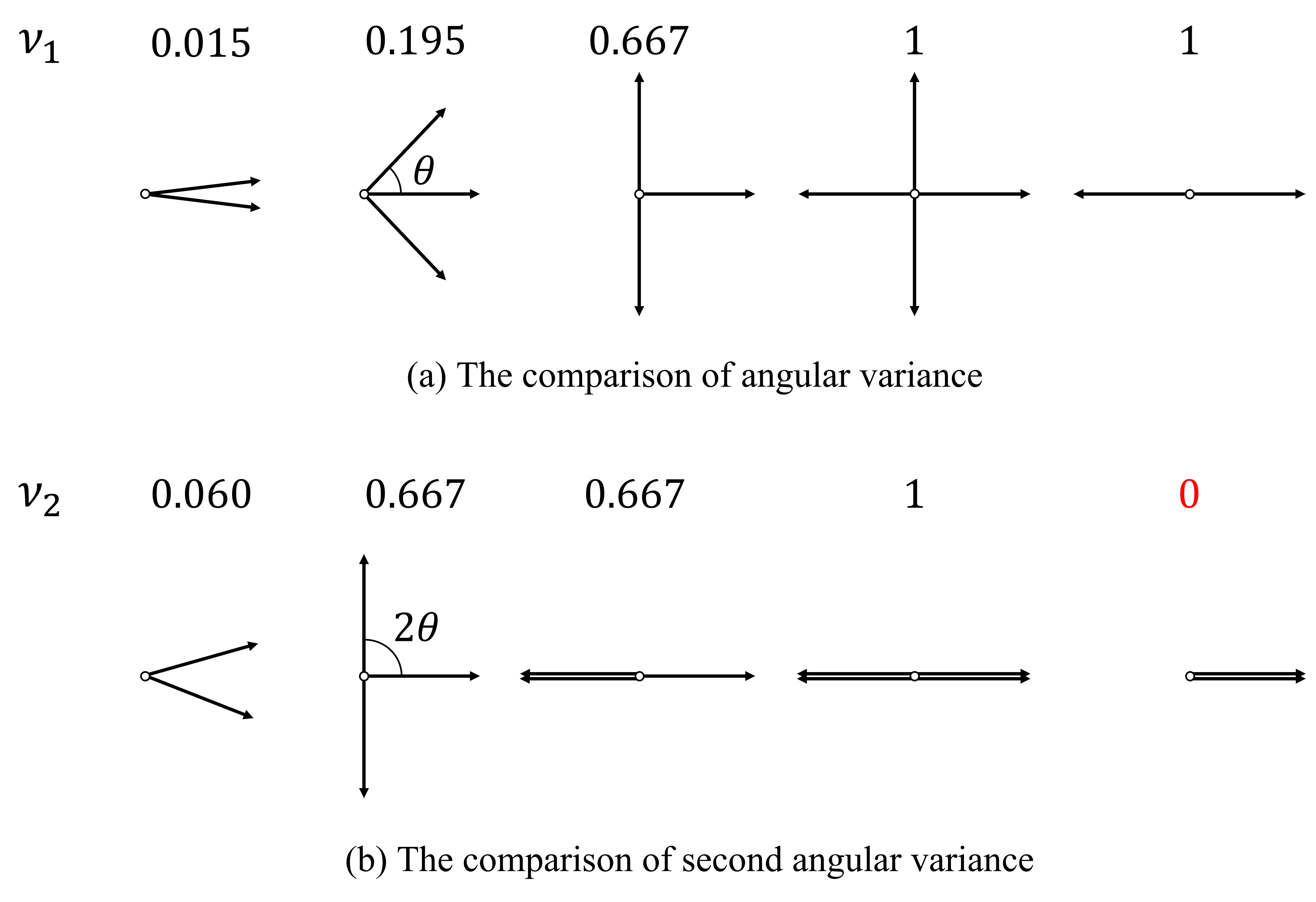
Figure 2: The comparison of angular variance and second angular variance.

3.2 $p$th angular variance

The angular variance cannot distinguish data with two peaks and four peaks in opposite directions as shown in the right two examples of Figure 2(a).

To distinguish these data quantitatively, we define a novel statistic, the $p$th angular variance, $\nu_{p}$ as

$$\nu_{p}=1-\bar{R}_{p},$$ (5)

where,

$$\bar{R}_{p}=\sqrt{\bar{C}_{p}^{2}+\bar{S}_{p}^{2}},$$ (6)

$$\bar{C}_{p}=\frac{1}{N}\sum_{j=1}^{N}\cos p\theta_{j},\quad\bar{S}_{p}=\frac{1}{N}\sum_{j=1}^{N}\sin p\theta_{j}.$$ (7)

$p$ is an exogenous variable that can take any natural number.

$\nu_{p}$ is derived by multiplying the angular data by $p$ and calculating the angular variance. $\nu_{p}$ gets a smaller value for the distribution with peaks every period $2\pi/p$. For example, as shown in Figure 2(b), the second angular variance is $0$ for data with two peaks, while it is still 1 for the data with four peaks.

Table 1 shows the value of $p$th angular variance $\nu_{p}$ $(p=1,2,3,4)$ for each flow type. The flow type and its distribution of movement directions were shown in Figure 1. The angular variance $\nu_{1}$ of uni-directional flow takes a value close to 0. In contrast, ones of bi-directional flow and crossing-A flow takes values close to 1. In addition, the one of crossing-B flow has a relatively smaller value than bi-directional flow and crossing-A flow because the interval between peaks is narrow. The second angular variance $\nu_{2}$ of bi-directional flow and the fourth angular variance $\nu_{4}$ of crossing-A flow take small values while the angular variances $\nu_{1}$ of these flows are large. Therefore, the $p$th angular variance can be confirmed to take a small value when the angular data had peaks every $2\pi/p$ period.

The four flow types can be distinguished by a combination of $\nu_{1}$ and $\nu_{2}$ without using a higher degree of angular variances. The uni-directional flow has small angular variance $\nu_{1}$ and a small second angular variance $\nu_{2}$, bi-directional flow has large $\nu_{1}$ and small $\nu_{2}$, crossing-A flow has large $\nu_{1}$ and large $\nu_{2}$ and crossing-B flow has relatively small $\nu_{1}$ and large $\nu_{2}$. Therefore, the four flow types can be distinguished by the angular variance $\nu_{1}$ and the second angular variance $\nu_{2}$.

Table 1: Angular variance of the distribution of pedestrian movement directions for each flow type shown in Figure 1.

Flow type	$\nu_{1}$	$\nu_{2}$	$\nu_{3}$	$\nu_{4}$
Uni-directional	0.013	0.052	0.112	0.187
bi-directional	0.958	0.166	0.975	0.514
Crossing-A	0.958	0.947	0.931	0.459
Crossing-B	0.303	0.944	0.407	0.245

3.3 Formulation of FD

Note that in the following discussion, $J$ is the flow, $u$ is the free flow speed, $\rho$ is the density and $C$ is the capacity.

3.3.1 Base function

In free flow state where $u\rho<C$, the flow $J$ equals $u\rho$ and increases linearly with the density $\rho$. In congested state where $u\rho>C$, the flow $J$ equals the capacity $C$ which is constant to simplify the model. Under these conditions, the simple pedestrian FD models can be described as

$$J=\min(u\rho,C).$$ (8)

This simplification is justified by the fact that the slopes of FDs in congested state are smaller than that of free flow state in many models [11]. The extreme congestion state where flow decreases as density increases is omitted because it cannot be seen in data.

Note that in this study, the flow $J$ is assumed to be constant in the congested state independent of the density $\rho$. In other words, the FDs like triangular FDs where the flow $J$ decreases as the density $\rho$ increases are not discussed. In the flow-density plots of pedestrians, the decline of flow $J$ in the congested state is not observed for multi-directional flow [11][18][19][25], and the same tendency is observed in the data used in this study. Therefore, the flow rate $J$ in the congested state is assumed to be constant in this study modeling FD of pedestrian flows, including multi-directional flows.

3.3.2 Incorporating $p$th angular variance into FD function

In the following, angular variance is incorporated into the model to represent the effects of the avoidance of conflicts on pedestrian flows. When pedestrian flows cross, the flow decreases due to the avoidance. The avoidance is expected to occur primarily at high density, i.e., in congested state. Therefore, the avoidance of conflicts is assumed to affect capacity $C$.

First, the effect of avoidance of conflicts is modeled. If pedestrians flow uni-directional, the effect seems to be small. In this case, the distribution of the direction of pedestrians has a single peak. On the other hand, if pedestrians flow multi-directional, the effect seems to be large. In this case, the distribution of the direction of pedestrians does not have a single peak clearly. As described in section 3.1, the degree of dispersion in the direction of the pedestrian can be described by angular variance $\nu_{1}$. Therefore, the magnitude of the capacity $C$ reduction due to avoidance of conflicts is controlled by angular variance $\nu_{1}$ in the proposed model.

Next, the effect of lane formation is modeled. Lane formation occurs in bi-directional flow. For bi-directional flow, the second angular variance $\nu_{2}$ takes a small value because the distribution of the direction of pedestrians has two peaks with a period of $\pi$. Since the capacity $C$ is expected to decrease when lane formation does not occur, the capacity $C$ decreases as the second angular variance $\nu_{2}$.

3.3.3 Incorporating the effects of the walls into FD function

Additionally, the model incorporates the effect of surrounding walls within the observation area. When walls are placed in the travel area, pedestrians move to avoid conflicting walls. Therefore, movement in an area surrounded by walls is expected to be less efficient. To quantify the effect of walls, we defined a metric termed the wall ratio $r$ as,

$$r=\frac{L-l}{L},$$ (9)

where $L$ denotes the total perimeter of the measurement area and $l$ denotes the length of the passable pedestrian section within it. For example, as shown in Figure 3 when square measurement areas are assumed, $r$ equals 0.5 for a corridor and $r$ equals 0 for a crossing. In the model, the capacity $C$ is assumed to decrease with the wall ratio $r$ increasing.

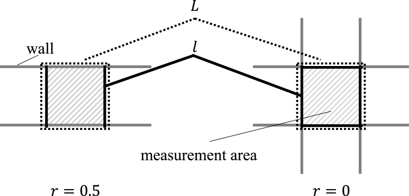
Figure 3: Examples of wall ratio $r$.

3.3.4 Proposed FD model

Based on the discussion in section 3.3.2 and 3.3.3, the capacity $C$ is assumed to decrease due to angular variance $\nu_{1}$, the second angular variance $\nu_{2}$, and wall ratio $r$. Therefore, the capacity is expressed as

$$C=C_{0}(1-\gamma_{1}\nu_{1}-\gamma_{2}\nu_{2})(1-\gamma_{\mathrm{wall}}r),$$ (10)

where $C_{0}$ represents the capacity without the effects of $\nu_{1}$, $\nu_{2}$ and $r$. $\gamma_{1},\gamma_{2}$ and $\gamma_{\mathrm{wall}}$ are parameters. From now on, the term of $(1-\gamma_{1}\nu_{1}-\gamma_{2}\nu_{2})(1-\gamma_{\mathrm{wall}}r)$ is called capacity penalty.

Substituting Eq. (10) into Eq. (8), an FD model of the pedestrian flows that takes into account the effects of flow types and the wall is obtained as

$$J=\min(u\rho,C_{0}(1-\gamma_{1}\nu_{1}-\gamma_{2}\nu_{2})(1-\gamma_{\mathrm{wall}}r)).$$ (11)

Since Eq. (11) uses the minimum function, there are indifferentiable points. To simplify handling in numerical processing such as estimation, Eq. (11) is smoothed by applying the log-sum-exp (LSE) function [29] defined as

$$\mathrm{LSE}(x_{1},x_{2},\ldots,x_{n}) \equiv\log\left(\sum_{j=1}^{i}\exp(x_{i})\right)$$

$$\thickapprox\max(x_{1},x_{2},\ldots,x_{n}).$$ (12)

LSE function is a smooth approximation of the maximum function. It can also approximate the minimum function by interchanging the signs as

$$-\mathrm{LSE}(-x_{1},-x_{2},\ldots,-x_{n}) \thickapprox-\max(-x_{1},-x_{2},\ldots,-x_{n})$$

$$=\min(x_{1},x_{2},\ldots,x_{n}).$$ (13)

The pedestrian FD model proposed in this study is completed by applying the LSE function with the signs switched to Eq. (11) as

$$J(\rho,\nu_{1},\nu_{2},r)=-\log\{\exp(-u\rho)+\exp\left(-C_{0}(1-\gamma_{1}\nu_{1}-\gamma_{2}\nu_{2})(1-\gamma_{\mathrm{wall}}r)\right)\}.$$ (14)

Figure 4 shows a schematic diagram of the models described in this section.

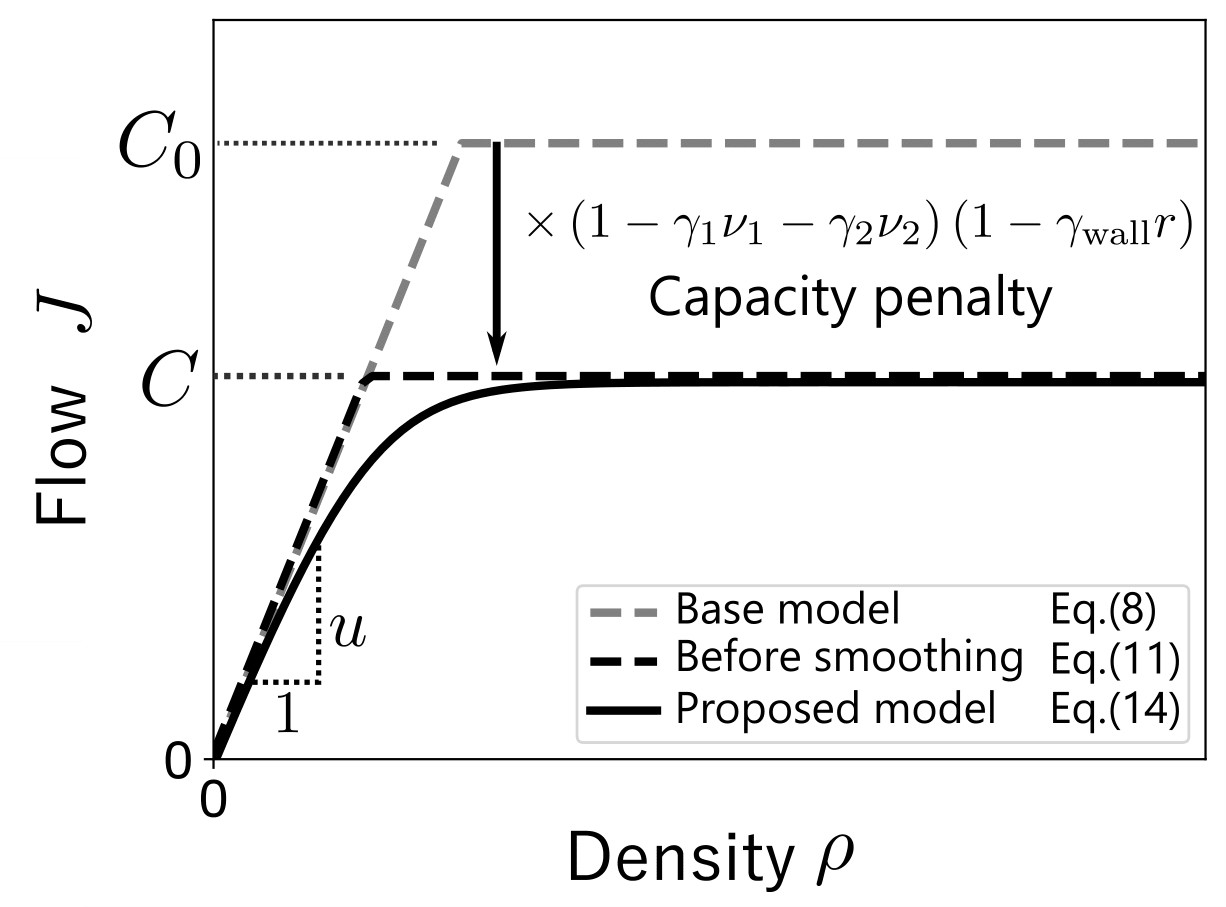
Figure 4: Schematic diagram of the models.

4 Case study

4.1 Data

We used “Unidirectional pedestrian flow in a corridor” dataset (DOI: 10.34735/ped.2013.6), “Bidirectional pedestrian flow in a corridor” dataset (DOI: 10.34735/ped.2013.5) and “Pedestrian flow at a 90 degree crossing” dataset (DOI: 10.34735/ped.2013.4). They are provided by a German research institute, Forschungszentrum Jülich. These three datasets correspond to four flow types: uni-directional flow, bi-directional flow, crossing-A flow, and crossing-B flow, defined in Section 1. The data contains the pedestrian’s coordinates and ID for each frame. The frame rates are 25 fps or 16 fps, depending on the dataset.

Figure 5: Top view photograph of one of the bi-directional flow experiment (Source: https://ped.fz-juelich.de/da/doku.php?id=corridor6).

The flow $J$ and the density $\rho$ are calculated from the trajectory data. They were obtained by applying the Edie’s definition [30] as

$$J=\frac{\sum_{s}d_{s}}{A},$$ (15)

and

$$\rho=\frac{\sum_{s}t_{s}}{A},$$ (16)

respectively. $A$ is the spatio-temporal region in which the flow and density are measured. The time region was set to 10 seconds, and the spatial region was set to square areas in the center of the corridor or crossing. $d_{s}$ represents the distance that pedestrian $s$ has traveled in spatio-temporal region $A$, and $t_{s}$ represents the travel time in the region. The flow $J$ and the density $\rho$ at time $\tau$ were calculated in the following way.

1. The coordinates of the pedestrians in the measurement area at time $\tau$ are obtained from the data.

2. The number of pedestrians in the measurement area multiplied by the interval for calculating (1 second) was added to $\sum_{s}t_{s}$.

3. The displacements for all pedestrians in the measurement area were calculated from the coordinates of the pedestrians after 1 second. They were added to $\sum_{s}d_{s}$.

4. Steps 1 to 3 were repeated for 10 seconds while increasing the time by 1 second.

5. The flow $J$ and density $\rho$ were calculated by Eq. (15) and Eq. (16)

The interval for calculating the displacement was set as long as 1 second. By taking a long interval, short movements in unintended directions due to the avoidance of conflicts were not added to the flow.

Figure 6 shows a scatter plot of the calculated flow $J$ and density $\rho$ for four flow types. The capacity of the FD is different depending on the flow types. Therefore, explaining this data with a single equation is difficult with existing models.

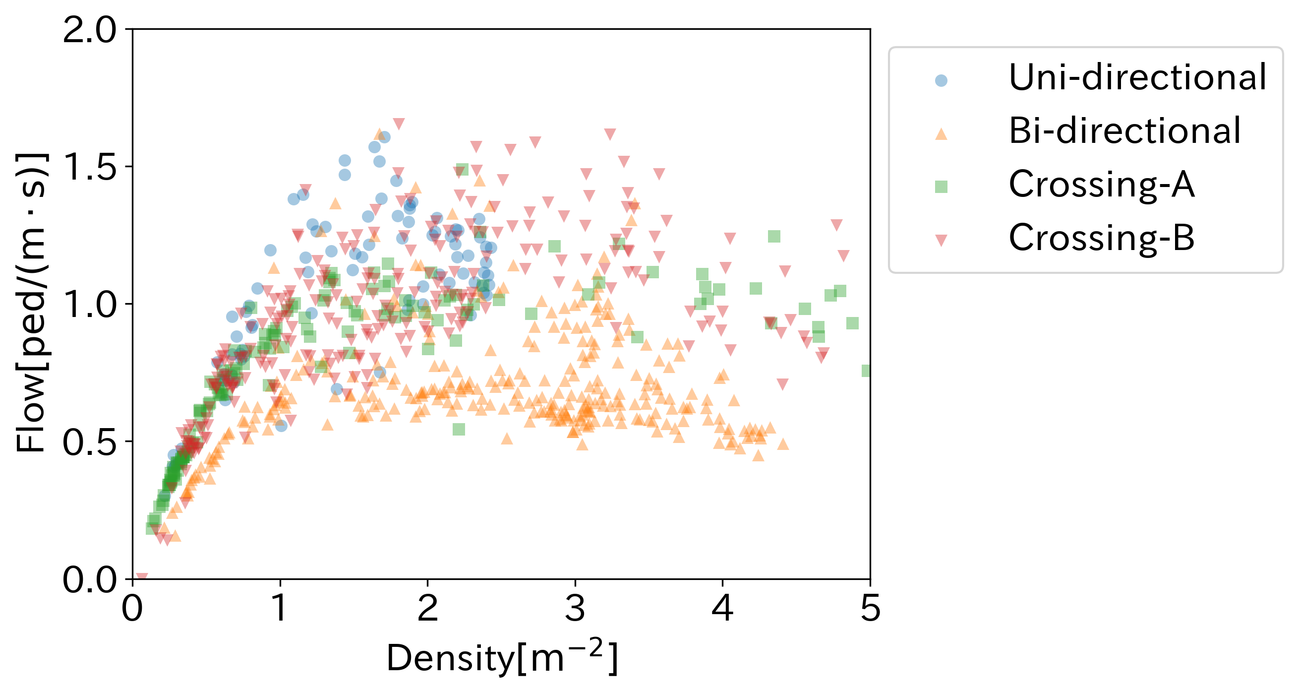
Figure 6: Flow-density plots of calculated data.

The angular variance $\nu_{1}$ and the second angular variance $\nu_{2}$ at time $\tau$ were calculated in the following way.

1. The coordinates of the pedestrians in the measurement area at time $\tau$ are obtained from the data.

2. Angles of pedestrians were calculated by comparing with the coordinates after 0.2 (for 25 fps data) or 0.25 (for 16 fps data) seconds.

3. Steps 1 to 2 were repeated for 10 seconds while increasing the time by 0.2 or 0.25 seconds.

4. $\nu_{1}$ and $\nu_{2}$ were calculated using all the angles computed during the 10 seconds by Eq. (2) and Eq. (5).

In order to evaluate the avoidance of conflicts by angular variance, the intervals were set to short enough to pick up small movements.

The wall ratio $r$ was calculated according to the definition given in Eq. (9), with $r=0.5$ for uni-directional and bi-directional flows and $r=0$ for crossing flows.

The flow $J$, the density $\rho$, the angular variance $\nu_{1}$, the second angular variance $\nu_{2}$, and the wall ratio $r$ were calculated every 10 seconds according to the above procedure. For each flow type, 80 sets of the variables at random time intervals were sampled, of which 50 were set as training data and 30 as test data.

4.2 Parameter estimation

The parameters of the model were estimated using the training data. The data for all flow types were applied simultaneously to obtain the parameters that fit all flow types. The least squares method was employed for the estimation. Table 2 shows the parameter estimation results.

Table 2: Estimation results.

	Coefficient	$t$ value	$p$ value
$u$[m/s]	3.092	18.541	$<10^{-10}$
$C_{0}$[ped/(m$\cdot$s)]	1.527	15.243	$<10^{-10}$
$\gamma_{1}$	0.224	6.199	$3.345\times 10^{-9}$
$\gamma_{2}$	0.210	3.372	$8.992\times 10^{-4}$
$\gamma_{\mathrm{wall}}$	0.435	4.736	$4.204\times 10^{-6}$

Table 3 shows the value of the coefficients of determination $R^{2}$ and adjusted coefficients of determination $\bar{R}^{2}$ for the training and test data. The coefficient of determination was approximately 0.6, indicating that this model can explain flow $J$ of different flow types to some extent.

Table 3: Coefficient of determination of the proposed model.

	$R^{2}$	$\bar{R}^{2}$
Train data	0.654	0.646
Test data	0.615	0.599

4.3 Discussion

According to the estimation results in Table 2, the signs of the estimates of $\gamma_{1}$, $\gamma_{2}$, and $\gamma_{\mathrm{wall}}$ were positive. This is consistent with the assumption in Section 3 that the larger angular variance $\nu_{1}$, the second angular variance $\nu_{2}$, and the wall ratio $r$ decrease the capacity $C$. In addition, all parameters were significant according to the $t$ values and $p$ values.

Figure 7 shows the estimated FD and plots of samples on the flow-density plane. The FD drawn as the solid line is the case without any capacity penalty where the angular variance $\nu_{1}$, the second angular variance $\nu_{2}$, and wall ratio $r$ are all $0$, i.e., the capacity $C$ equals $C_{0}$. As the capacity penalty increases, the FD moves down from the solid line. The domain is colored according to the magnitude of the capacity penalty. On the other hand, the dots indicating the samples with the flow and density for a particular 10-second period are also colored by their capacity penalty. Therefore, when the color of a dot and the surrounding area are similar, it implies a favorable estimation result for that sample.

According to Figure 7, most light-colored dots with a small penalty are located in the light domain, and most dark-colored dots with a large penalty are located in the dark domain. In addition, the results for each flow type identified by the dots’ shapes also show a similar color match between the dots and the surrounding domain for all four types. This indicates that the proposed model performs well for data with a mixture of several flow types.

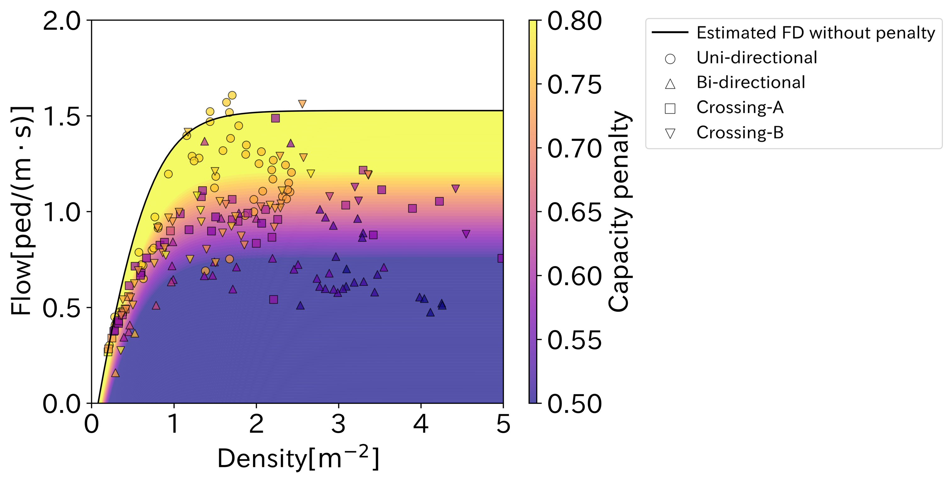
Figure 7: Flow-density plots of (the 50 training data) $\times$ (4 flow types) and the estimated FD colored according to the value of capacity penalty $(1-\gamma_{1}\nu_{1}-\gamma_{2}\nu_{2})(1-\gamma_{\mathrm{wall}}r)$.

Figure 8 compares the estimated flow and the actual flow for each sample. In the left figure, the estimated flow is derived by the model without angular variance $\nu_{1}$ and second angular variance $\nu_{2}$, which corresponds to the equation

$$J=-\log\{\exp(-u\rho)+\exp\left(-C_{0}(1-\gamma_{\mathrm{wall}}r)\right)\}.$$ (17)

From now on, the model Eq. (17) is called simple model. Each sample is colored by the value of angular variance $\nu_{1}$ in Figure 8(a) and the one of second angular variance $\nu_{2}$ in Figure 8(b).

Flows that were estimated to be close to $1.0$ in the simple model are separated in the proposed model, and the accuracy of the fit becomes relatively improved. This is also confirmed by comparing the coefficient of determination for the simple model shown in Table 4 and the proposed models shown in Table 3. In concrete, uni-directional flows with an actual flow distributed between $1.0$ and $1.5$ colored by blue in both figures are separated from the other flow types. The flow is estimated to be larger in the uni-directional flow because the angular variance $\nu_{1}$ and the second angular variance $\nu_{2}$ are smaller. Furthermore, Figure 7(b) shows that the bi-directional flow drawn by the triangular dots is concentrated around $(\text{Actual flow},\text{Estimated flow})=(0.6,1)$ in the simple model, while they are separated by the value of second angular variance $\nu_{2}$ in the proposed model. This implies that the lane formation of the bi-directional flow can be represented to a certain extent by the second angular variance $\nu_{2}$. These indicate that incorporating the angular variance $\nu_{1}$ and the second angular variance $\nu_{2}$ contribute to simultaneously estimating the pedestrian FD of several flow types.

Table 4: Coefficient of determination of the simple model.

	$R^{2}$	$\bar{R}^{2}$
Train data	0.451	0.443
Test data	0.484	0.470

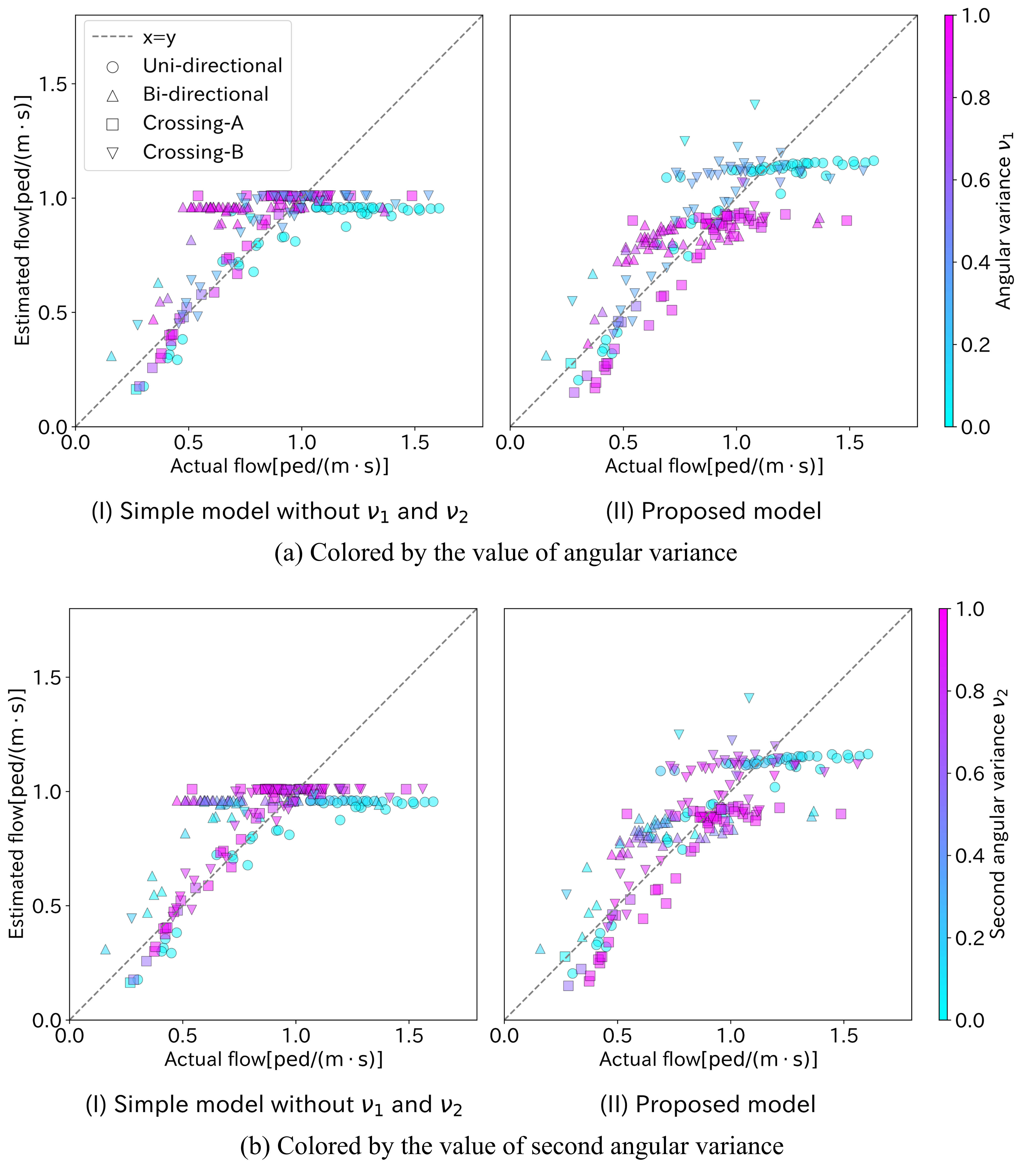
Figure 8: Scatter plots with actual flow on the horizontal axis and the estimated flow on the vertical axis for each model with colored by the value of angular variance $\nu_{1}$ or that of second angular variance $\nu_{2}$.

5 Conclusion

We proposed a comprehensive model of pedestrian FDs that can be applied to various flow types. Specifically, we employ the angular variance to characterize the flow types, such as uni-directional, bi-directional, and crossing flow. It enables the FDs to explain the effect of flow types on flow performance, such as efficient bi-directional flows and inefficient crossing flows. The model was estimated and validated using actual pedestrian trajectory data. The estimated values of the parameters were consistent with the assumptions of the modeling. The capacities of estimated FD varied based on the effect of avoidance of conflicts, measured by angular variance and the second angular variance. This implies that pedestrian flow characteristics can be depicted using Directional Statistics.

The current model is still simple and has several limitations, as it is the first attempt of this kind. First, the proposed model does not describe the congested part of an FD. This is because congested pedestrian flow is completely different from free-flowing or saturated flows, and experimental data is very limited. Second, although it predict average flow based on directional-dependent flow, it does not predict direction-dependent flow itself (i.e., input is directional-dependent, but the output is not). To extend the proposed model to directional-dependent flow prediction, the approach developed by Nagasaki and Seo [8] could be utilized. Case studies with other datasets with different geometries such as in T-junctions or open spaces are also considerable to confirm the generality of the proposed methodology.

CRediT author statement contribution statement

Keiichiro Fujiya: Conceptualization; Data curation; Formal analysis; Investigation; Methodology; Validation; Visualization; Writing - original draft. Kota Nagasaki: Conceptualization; Formal analysis; Investigation; Methodology; Validation; Visualization; Writing - review & editing. Toru Seo: Conceptualization; Funding acquisition; Methodology; Project administration; Resources; Supervision; Visualization; Writing - review & editing.

Declaration of competing interest

The authors declare that there are no known competing interest.

Declaration of generative AI and AI-assisted technologies in the writing process

During the preparation of this work the authors used GPT-4 for a grammatical proofreading purpose. After using this tool/service, the authors reviewed and edited the content as needed and takes full responsibility for the content of the publication.

References

- [1] L. D. Vanumu, K. Ramachandra Rao, G. Tiwari, Fundamental diagrams of pedestrian flow characteristics: A review, European Transport Research Review 9 (4) (2017) 1–13. doi:10.1007/s12544-017-0264-6.
- [2] A. D. May, Traffic Flow Fundamentals, Prentice Hall, New Jersey, 1989.
- [3] C. Feliciani, K. Nishinari, Empirical analysis of the lane formation process in bidirectional pedestrian flow, Physical Review E 94 (3) (2016) 032304. doi:10.1103/PhysRevE.94.032304.
- [4] K. V. Mardia, P. E. Jupp, K. V. Mardia, Directional Statistics (1999).
- [5] R. A. Johnson, T. E. Wehrly, Some Angular-Linear Distributions and Related Regression Models, Journal of the American Statistical Association 73 (363) (1978) 602–606. arXiv:2286608, doi:10.2307/2286608.
- [6] J. T. Schnute, K. Groot, Statistical analysis of animal orientation data, Animal Behaviour 43 (1) (1992) 15–33. doi:10.1016/S0003-3472(05)80068-5.
- [7] G. Boeing, Urban spatial order: Street network orientation, configuration, and entropy, Applied Network Science 4 (1) (2019) 67. doi:10.1007/s41109-019-0189-1.
- [8] K. Nagasaki, T. Seo, Understanding Impact of Angle in Urban Transportation (Oct. 2023). arXiv:2310.16470, doi:10.48550/arXiv.2310.16470.
- [9] K. Nagasaki, W. Nakanishi, Y. Asakura, Application of the rose diagram to road network analysis, in: 24th International Conference of Hong Kong Society for Transportation Studies, Hong Kong, 2019.
- [10] J. J. Fruin, DESIGNING FOR PEDESTRIANS: A LEVEL-OF-SERVICE CONCEPT, in: Highway Research Record, no. HS-011 999, 1971.
- [11] M. R. Virkler, S. Elayadath, Pedestrian speed-flow-density relationships, Transportation research record 1438 (1994) 51–58.
- [12] A. Seyfried, B. Steffen, W. Klingsch, M. Boltes, The fundamental diagram of pedestrian movement revisited, Journal of Statistical Mechanics: Theory and Experiment 2005 (10) (2005) P10002. doi:10.1088/1742-5468/2005/10/P10002.
- [13] J. Zhang, A. Seyfried, Empirical Characteristics of Different Types of Pedestrian Streams, Procedia Engineering 62 (2013) 655–662. doi:10.1016/j.proeng.2013.08.111.
- [14] W. H. K. Lam, J. Y. S. Lee, C. Y. Cheung, A study of the bi-directional pedestrian flow characteristics at Hong Kong signalized crosswalk facilities, Transportation 29 (2) (2002) 169–192. doi:10.1023/A:1014226416702.
- [15] C.-J. Jin, R. Jiang, S. C. Wong, S. Xie, D. Li, N. Guo, W. Wang, Observational characteristics of pedestrian flows under high-density conditions based on controlled experiments, Transportation Research Part C: Emerging Technologies 109 (2019) 137–154. doi:10.1016/j.trc.2019.10.013.
- [16] X. Jia, H. Murakami, C. Feliciani, D. Yanagisawa, K. Nishinari, Pedestrian lane formation and its influence on egress efficiency in the presence of an obstacle, Safety Science 144 (2021) 105455. doi:10.1016/j.ssci.2021.105455.
- [17] J. Lee, T. Kim, J.-H. Chung, J. Kim, Modeling lane formation in pedestrian counter flow and its effect on capacity, KSCE Journal of Civil Engineering 20 (3) (2016) 1099–1108. doi:10.1007/s12205-016-0741-9.
- [18] J. Zhang, A. Seyfried, Comparison of intersecting pedestrian flows based on experiments, Physica A: Statistical Mechanics and its Applications 405 (2014) 316–325. doi:10.1016/j.physa.2014.03.004.
- [19] S. Cao, A. Seyfried, J. Zhang, S. Holl, W. Song, Fundamental diagrams for multidirectional pedestrian flows, Journal of Statistical Mechanics: Theory and Experiment 2017 (3) (2017) 033404. doi:10.1088/1742-5468/aa620d.
- [20] M. Iryo, A. Nagashima, Performance Evaluation of Pedestrian Crossing Flow, Seisan-kenkyu 67 (4) (2015) 369–373. doi:10.11188/seisankenkyu.67.369.
- [21] D. Helbing, P. Molnár, Social force model for pedestrian dynamics, Physical Review E 51 (5) (1995) 4282–4286. doi:10.1103/PhysRevE.51.4282.
- [22] M. Asano, T. Iryo, M. Kuwahara, A Pedestrian Model Considering Anticipatory Behaviour for Capacity Evaluation, in: W. H. K. Lam, S. C. Wong, H. K. Lo (Eds.), Transportation and Traffic Theory 2009: Golden Jubilee: Papers Selected for Presentation at ISTTT18, a Peer Reviewed Series since 1959, Springer US, Boston, MA, 2009, pp. 559–581. doi:10.1007/978-1-4419-0820-9_28.
- [23] M. Moussaïd, D. Helbing, S. Garnier, A. Johansson, M. Combe, G. Theraulaz, Experimental study of the behavioural mechanisms underlying self-organization in human crowds, Proceedings of the Royal Society B: Biological Sciences 276 (1668) (2009) 2755–2762. doi:10.1098/rspb.2009.0405.
- [24] W. Nakanishi, T. Fuse, A preliminary study on analysis of pedestrian traffic line using angular data, JSTE Journal of Traffic Engineerin 1 (4) (2015) A18–A23.
- [25] G. Flötteröd, G. Lämmel, Bidirectional pedestrian fundamental diagram, Transportation Research Part B: Methodological 71 (2015) 194–212. doi:10.1016/j.trb.2014.11.001.
- [26] C. Feliciani, H. Murakami, K. Nishinari, A universal function for capacity of bidirectional pedestrian streams: Filling the gaps in the literature, PLOS ONE 13 (12) (2018) e0208496. doi:10.1371/journal.pone.0208496.
- [27] E. Moustaid, G. Flötteröd, Macroscopic model of multidirectional pedestrian network flows, Transportation Research Part B: Methodological 145 (2021) 1–23. doi:10.1016/j.trb.2020.12.004.
- [28] G. Flötteröd, J. Rohde, Operational macroscopic modeling of complex urban road intersections, Transportation Research Part B: Methodological 45 (6) (2011) 903–922.
- [29] F. Nielsen, K. Sun, Guaranteed bounds on information-theoretic measures of univariate mixtures using piecewise log-sum-exp inequalities, Entropy 18 (12). doi:10.3390/e18120442.
- [30] L. Edie, Discussion of traffic stream measurements and definitions, in: 2nd International Symposium on the Theory of Traffic Flow, London, 1963.