Remote Nucleation and Stationary Domain Walls via Transition Waves
in Tristable Magnetoelastic Lattices

Abstract

We present a tunable magnetoelastic lattice with a multistable onsite potential, focusing on a tristable potential. Through experimental and numerical analysis, we verify the existence of three types of transition waves with distinct amplitudes and velocities. Additionally, we establish the presence of a scaling law that elucidates various characteristics of these transition waves. By manipulating the onsite potential, we investigate the collision dynamics of two transition waves within the system. In chains featuring an asymmetric potential well, the collision of similar transition waves leads to the remote nucleation of a new phase. In chains with a symmetric potential well, the collision of dissimilar transition waves results in the formation of a stationary domain wall.

Introduction

Investigating transition waves is crucial for understanding dislocation dynamics [1] and phase transitions in various advanced materials, including ferroelectric [2], ferromagnetic [3], and shape memory alloys [4]. These waves have been extensively studied theoretically on lattices possessing nonconvex energy landscapes with multiple stable equilibria [5, 6, 7, 8, 9, 10, 11, 12, 13]. Within such systems, transition waves manifest as moving phase boundaries or domain walls, facilitating the transition between stable equilibria as they propagate through the material.

Similar phenomena have emerged in metamaterials in recent years, where macroscopic mechanical systems exhibit multiple stable equilibria [14, 15]. By finely adjusting potentials and degrees of freedom, precise control over transition waves is achieved in metamaterials, enabling the design of reconfigurable structures with applications in soft robotics [16, 17], energy absorption [18], deployable structures [19], and sound control [20, 21].

Initially, research into transition waves in metamaterials primarily focused on bi-stable unit cells with asymmetry sufficient to compensate for the system damping and make the transition wave robust [22, 23, 24, 25, 26, 27]. However, recent investigations have explored metamaterials with tristable configurations featuring three stable equilibria [28, 29]. Notable findings include the observation of stationary domain wall formation resulting from the collision of two transition waves [28] – a mechanism distinct from that in bistable lattices, which require additional defects to form a stationary domain wall [30, 31]. Additionally, the nucleation of a new phase away from metamaterial’s boundaries was observed following the collision of two weakly nonlinear vector solitons [29]. These functionalities promise to enhance the reconfigurability of metamaterials in various practical scenarios. For instance, the formation of stationary domain walls at different spatial locations enables the maintenance of desired phase mixtures, thereby modulating the effective stiffness of the metamaterial. Moreover, nucleating a new phase within the metamaterial could be advantageous in scenarios where a single dynamic actuation from one boundary is insufficient to initiate the transition. Instead, a spatially distributed dynamic actuation could be used for collectively inducing phase transitions by superposing their individual responses.

However, previous studies on tristable metamaterials relied on rotating square lattices, inducing a multi-stable energy landscape of intersite potential [28, 29]. The comprehensive exploration of the dynamics inherent in tristable metamaterials featuring onsite potential remains largely unaddressed within current scientific literature. Moreover, stationary domain walls and remote nucleation have not been observed in a single system, as hinge thickness in rotating square mechanisms must be varied to tune the energy landscape. Additionally, the nucleation relied on the collision of two weakly nonlinear waves, i.e., vector solitons (not transition waves); therefore, material dissipation and system size may diminish their energy before the collision, leading to the absence of nucleation. This highlights the need for designing a metamaterial that addresses three key issues: (1) having a tristable energy landscape for onsite potential, (2) offering tunability in energy well for the formation of stationary domain wall and nucleation, and (3) providing a robust way to remotely nucleate a new phase deep within the boundaries of the metamaterial.

Therefore, we propose a magnetoelastic lattice comprising elastic elements and permanent magnets that provide tunable onsite potential. By adjusting the positions of permanent magnets, we demonstrate experimentally and numerically that the lattice can exhibit monostable, bistable, or tristable behavior. Specifically, the tristable lattice, with designed asymmetry, supports three types of transition waves. Furthermore, we experimentally verify a scaling law relating transition wave velocity to power dissipation due to damping [32]. We also show that two transition waves initiated from opposite ends can collide within the lattice, nucleating a third phase. Finally, by adjusting the spatial configurations of the permanent magnets, we achieve a symmetric tristable potential and experimentally demonstrate that two transition waves initiated from opposite ends collide, forming a stationary domain wall within the lattice.

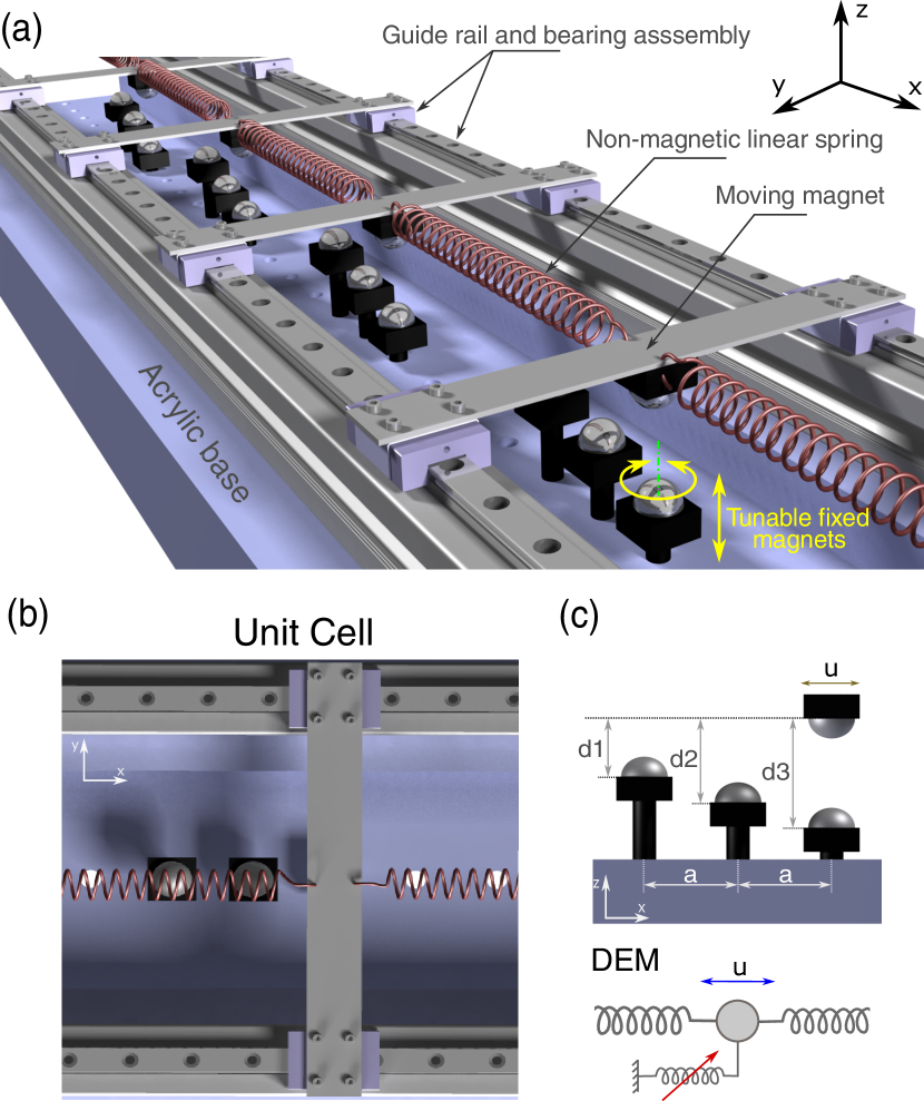
Figure 1: Experimental setup. (a) One-dimensional lattice assembly where the onsite potential is induced by fixed magnets. Moving masses are the sliding beams. (b) Top view of the unit cell, comprising three fixed magnets and one moving magnet attached beneath the sliding beam. (c) As per the discrete element model (DEM), the depths of the fixed magnets $(d_{1},d_{2},$ and $d_{3})$ create a multi-stable onsite potential for the moving magnet.

Experimental setup

We design a lattice comprising 10 unit cells, each consisting of a sliding beam (aluminum) connected to its neighbors via axial springs (phosphor-bronze), as depicted in Fig. 1. The structure rests on a solid acrylic base supported by a pair of aluminum extrusions, housing the linear guide rail and bearing assembly (MGN7C, HIWIN). Underneath each beam is a Neodymium (N-52) permanent magnet, referred to as a “moving magnet”, as it moves along the $x$-axis with the beam. Three magnets are affixed to the acrylic base for each unit cell, spaced at a distance $a=20$ mm between them. All the permanent magnets are spherical and uniformly magnetized along the out-of-plane direction, or $z$-axis, with a radius of $r=5$ mm. The unit cells are adequately spaced, with a distance $l=120$ mm between them, ensuring that the moving magnets primarily interact with the three fixed magnets within their respective unit cells. By individually rotating the fixed magnets, we alter their depths ($d_{1}$, $d_{2}$, and $d_{3}$), thus adjusting the effective onsite potential experienced by the moving magnet. For the measurements, we employ a Laser Doppler Vibrometer (Polytec single-point LDV) to detect the displacement of each moving mass.

Numerical modeling

.1 Nonlinear onsite potential

First, we model the magnetic interaction between moving and stationary magnets within a unit cell. Since all magnets possess uniform magnetization $m_{s}$ and are spherical with radius $r$, we derive the interaction energy, a function of $u$, the axial displacement of the moving mass, using Maxwell’s equations (refer to Supplemental Material for details):

$$\begin{split}E(u)=&\frac{4\pi m_{s}^{2}}{9\mu_{0}}r^{6}\Bigg{[}\Bigg{(}\frac{1}{((u+a)^{2}+d_{1}^{2})^{\frac{3}{2}}}-\frac{3d_{1}^{2}}{((u+a)^{2}+d_{1}^{2})^{\frac{5}{2}}}\Bigg{)}\\ &+\left(\frac{1}{(u^{2}+d_{2}^{2})^{\frac{3}{2}}}-\frac{3d_{2}^{2}}{(u^{2}+d_{2}^{2})^{\frac{5}{2}}}\right)\\ &+\left(\frac{1}{((u-a)^{2}+d_{3}^{2})^{\frac{3}{2}}}-\frac{3d_{3}^{2}}{((u-a)^{2}+d_{3}^{2})^{\frac{5}{2}}}\right)\Bigg{]},\end{split}$$ (1)

where $\mu_{0}=4\pi\times 10^{-7}\,\text{Vs/Am}$ denotes vacuum permeability. Magnetization of all N-52 magnets are considered as $m_{s}=0.8\,\text{T}$. Additionally, the depths of fixed magnets $d_{1}$, $d_{2}$, and $d_{3}$ are adjustable to modify the interaction energy landscape, as illustrated in Fig. 2. We maintain $d_{2}$ constant and examine the energy landscape’s behavior as $d_{1}$ and $d_{3}$ vary. Figure 2(a) demonstrates the possibility of monostable, bistable, and tristable potential landscapes for various depth combinations. We focus on the tristable regime, presenting two distinct tristable landscapes, one asymmetric and the other symmetric about $u=0$, depicted in Figs. 2(b)(i) and 2(b)(ii) respectively. In the later sections, we will analyze transition waves that facilitate system switching across three different phases (corresponding to three local minima), namely Phase 1, Phase 2, and Phase 3.

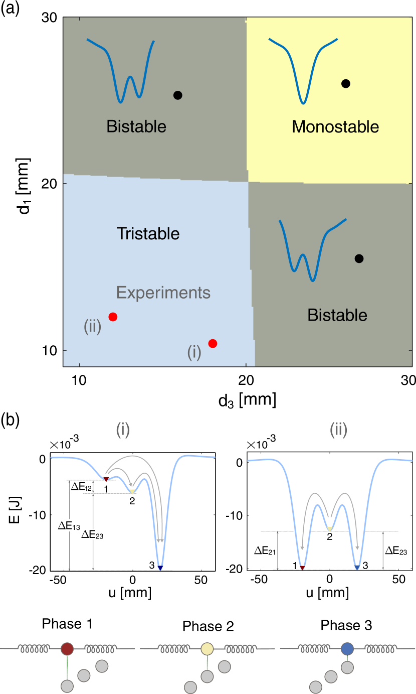
Figure 2: (a) Phase diagram of the onsite potential as function of $d_{1}$ and $d_{3}$, for fixed $a=20$ mm and ${d_{2}=15.3}$ mm. (b) Two tristable onsite potentials considered for experiments: (i) $(d_{1},d_{3})=(18,10.4)$ mm for an asymmetric well, (ii) $(d_{1},d_{3})=(12,12)$ mm for a symmetric well. Energy differences between different stable states are highlighted. Arrows denote different types of transition waves between Phase 1, Phase 2, and Phase 3.

.2 Equations of motion

We employ the discrete element method (DEM) to simulate the dynamics of our system. Sliding beams with moving magnets are treated as lumped masses interconnected by linear springs. To simplify calculations, we assume a significantly higher bending rigidity for the beams, neglecting out-of-plane motion along the $z$-axis for the moving mass. The derivative of the nonconvex onsite energy, previously calculated, serves as a measure of the onsite force acting on the moving magnets. Consequently, the equation of motion for the $n$th unit cell is given by:

$$\begin{split}&mu_{n,tt}-k(u_{n-1}-2u_{n}+u_{n+1})+E^{\prime}(u_{n})\\ &-c_{1}(u_{(n-1),t}-2u_{n,t}+u_{(n+1),t})+c_{2}\ \text{sgn}(u_{n,t})=0,\end{split}$$ (2)

where $m$ represents the mass of the moving assembly, $k$ denotes the linear stiffness of the springs, $c_{1}$ and $c_{2}$ are intersite and onsite damping parameters, respectively. Variables following a comma in indices denote partial derivatives. As the moving mass slides on the guide rails, we utilize a dry friction damping model for the onsite term and a viscous damping model for the springs.

.3 Scaling law for transition wave

In this section, we derive the scaling law for transition waves propagating in the system with velocity $\nu$. We thus assume $u_{n}(t)=u(nl-\nu t)\equiv u(\xi)$ and substitute it into Eq. (2) to yield

$$\begin{split}m\nu^{2}u_{,\xi\xi}-k\big{(}u(\xi-l)-2u(\xi)+u(\xi+l)\big{)}\\ +E^{\prime}(u)+c_{1}\nu\big{[}u_{,\xi}(\xi-l)-2u_{,\xi}(\xi)+u_{,\xi}(\xi+l)\big{]}\\ -c_{2}\nu\ \text{sgn}({u_{,\xi}})=0.\end{split}$$ (3)

Equations are thus transformed into a traveling frame of reference $\xi$. Multiplying Eq. (3) by $u_{,\xi}$ and integrating over the real $\xi$ axis, we obtain

$$\begin{split}\int_{-\infty}^{\infty}\bigg{[}m\nu^{2}u_{,\xi\xi}-k\big{(}u(\xi-l)-2u(\xi)+u(\xi+l)\big{)}\\ +E^{\prime}(u)\ +c_{1}\nu\big{(}u_{,\xi}(\xi-l)-2u_{,\xi}(\xi)+u_{,\xi}(\xi+l)\big{)}\\ -c_{2}\nu\ \text{sgn}({u_{,\xi}})\bigg{]}u_{,\xi}d\xi=0.\end{split}$$ (4)

If the transition wave changes the system from the initial phase $u_{i}$ at ${t\rightarrow-\infty}$ (${\xi\rightarrow\infty}$) to $u_{f}$ at ${t\rightarrow\infty}$ (${\xi\rightarrow-\infty}$), and hence we impose ${u(\xi\rightarrow\infty)=u_{i}}$ and ${u(\xi\rightarrow-\infty)=u_{f}}$. Furthermore, for a dissipative system, the wave profile would reach a steady state at ${t\rightarrow\infty}$, implying ${u_{,\xi}(\xi\rightarrow-\infty)=0}$. Since the system was initially at rest, we also have ${u_{,\xi}(\xi\rightarrow\infty)=0}$. Upon examining the individual integrals in Eq. (4), we find

$$\int_{-\infty}^{\infty}\left(m\nu^{2}u_{,\xi\xi}\right)u_{,\xi}d\xi=\int_{-\infty}^{\infty}\dfrac{m\nu^{2}}{2}\dfrac{d}{d\xi}\big{(}u_{,\xi}\big{)}^{2}d\xi=0.$$ (5)

Next we compute the integral

$$\mathcal{I}=\int_{-\infty}^{\infty}\left[k\left(u(\xi-l)-2u(\xi)+u(\xi+l)\right)\right]u_{,\xi}d\xi.$$

The second term of $\mathcal{I}$ reduced as

$$-2k\int_{-\infty}^{\infty}u(\xi)u_{,\xi}d\xi$$

$$=-k\int_{-\infty}^{\infty}\dfrac{d}{d\xi}\big{(}u({\xi})\big{)}^{2}d\xi=-k\big{(}u_{i}^{2}-u_{f}^{2}\big{)}.$$ (6)

We define $\eta=\xi-l$ and subsequently the first term of $\mathcal{I}$ can be rewritten as

$$\int_{-\infty}^{\infty}ku(\xi-l)u_{,\xi}(\xi)d\xi=\int_{-\infty}^{\infty}ku(\eta)u_{,\eta}(\eta+l)d\eta.$$ (7)

Since, $\eta$ is a dummy variable, this can be rewritten as

$$\int_{-\infty}^{\infty}ku(\eta)u_{,\eta}(\eta+l)d\eta=\int_{-\infty}^{\infty}ku(\xi)u_{,\xi}(\xi+l)d\xi.$$ (8)

Therefore, the first and the third terms of $\mathcal{I}$ are deduced to

$$\int_{-\infty}^{\infty} \left[k\left(u(\xi-l)+(\xi+l)\right)\right]u_{,\xi}d\xi$$

$$=k\int_{-\infty}^{\infty}\left[u(\xi)u_{,\xi}(\xi+l)+u(\xi+l)u_{,\xi}(\xi)\right]d\xi$$

$$=k\int_{-\infty}^{\infty}\dfrac{d}{d\xi}\left[u(\xi)u(\xi+l)\right]=k\big{(}u_{i}^{2}-u_{f}^{2}\big{)}.$$ (9)

Combining Eqs. (6) and  (9), the integral $\mathcal{I}=0$ . Finally, the term in Eq. (4)

$$\int_{-\infty}^{\infty}E^{\prime}(u)u_{,\xi}d\xi=E(u_{i})-E(u_{f})=\Delta E.$$ (10)

Therefore Eq. (4) reduces to

$$\begin{split}\Delta E=\int_{-\infty}^{\infty}\bigg{[}&-c_{1}\nu\big{(}u_{,\xi}(\xi-l)-2u_{,\xi}(\xi)+u_{,\xi}(\xi+l)\big{)}\\ &+c_{2}\nu\ \text{sgn}({u_{,\xi}})\bigg{]}u_{,\xi}d\xi.\end{split}$$ (11)

Multiplying both sides with $\nu/l$, approximating the right-hand side by a discrete system, we obtain

$$\begin{split}{\nu\Delta e}\simeq\sum_{n=1}^{N}\bigg{[}&-c_{1}\big{(}u_{n-1,t}-2u_{n,t}+u_{n+1,t}\big{)}\\ &+c_{2}\ \text{sgn}({u_{n,t}})\bigg{]}u_{n,t}\equiv P_{d}.\end{split}$$ (12)

where $\Delta e\equiv\Delta E/l$ represents the change in onsite energy per unit length. The right-hand side denotes the total power dissipated ($P_{d}$) by viscous and Coulomb damping. Due to discreteness, $P_{d}$ oscillates in time with a period $T=l/\nu$ (see Supplemental Material for details). Therefore, we compute the time-averaged $P_{d}$ as

$$\langle P_{d}\rangle=\frac{1}{T}\int_{t_{0}}^{t_{0}+T}P_{d}\ dt,$$ (13)

and we modify the scaling law as

$$\nu\Delta e\simeq\langle P_{d}\rangle.$$ (14)

A similar scaling law can be found in the work of Neel et al. [32]. However, we have validated this prediction for both non-linear onsite damping and linear intersite damping in our system. Since the power dissipated on the right-hand side is always positive due to the second law, we can conclude that $\nu\Delta e\geq 0$, which is analogous to the entropy condition derived in Ref. [7], with $\Delta e$ acting as the driving force on the phase boundary propagation. In our tristable lattice, the scaling remains independent of inter-particle stiffness. Furthermore, the specific topology of the onsite-site potential does not affect the scaling law; instead, it depends on the initial and final configuration of the energy state.

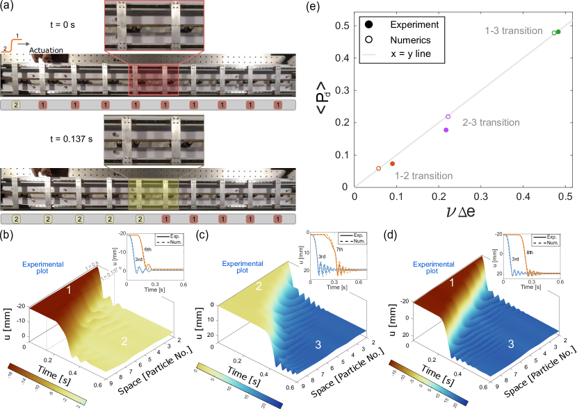
Figure 3: Three types of transition waves. (a) Snapshots from experiments demonstrating the $1\rightarrow 2$ transition wave. The unit cells are labeled with the phases. (b),(c),(d) Spatiotemporal plots of displacement obtained from experiments for $1\rightarrow 2$, $2\rightarrow 3$, and $1\rightarrow 3$ transition waves, respectively. Insets show the displacement time series of different moving masses. (e) Experimental validation of the scaling law in Eq. (14).

Results and Discussions

In this section, we present the numerical and experimental results for a tristable lattice comprising 10 unit cells.

Formation of transition waves

We perform experiments on a chain with an asymmetric tristable onsite potential, as depicted in Fig. 2(b)(i). Due to asymmetry in the well, we expect several robust transition waves propagating in the lattice. These wave profiles are also referred to as kinks or antikinks [33], and manifest as localized wave packets propagating with a constant shape. We identify three distinct types of transition waves: (i) $1\rightarrow 2$, with the transition from Phase 1 to Phase 2; (ii) $2\rightarrow 3$, with the transition from Phase 2 to Phase 3; and (iii) $1\rightarrow 3$, with the transition from Phase 1 to Phase 3.

First, we consider a scenario where all unit cells are in the highest energy state, i.e., Phase 1, and both ends of the chain are fixed. We then snap the first unit cell to Phase 2 and fix it while holding the second unit cell. This causes the spring between the first and the second unit cell to compress. We then release the second unit cell. Consequently, we observe a large-amplitude nonlinear wave propagating through the lattice, transitioning each unit cell from Phase 1 to Phase 2 as shown in Fig. 3(a). The spatiotemporal map of the displacement is plotted in Fig. 3(b), clearly indicating the propagation of the $1\rightarrow 2$ transition wave.

Similarly, we conduct experiments and observe $2\rightarrow 3$ and $1\rightarrow 3$ transition waves as shown in Fig. 3(c) and 3(d), respectively. To the best of the authors’ knowledge, the $1\rightarrow 3$ transition wave, which skips the intermediate stable state, has not been documented in the literature previously. We also observe that $1\rightarrow 2$, $2\rightarrow 3$, and $1\rightarrow 3$ transition waves reach the end of the chain approximately at time 0.32 s, 0.42 s, and 0.27 s, respectively. Therefore, we conclude that the $1\rightarrow 3$ transition wave has the highest velocity, whereas the $2\rightarrow 3$ transition wave exhibits the lowest velocity.

Experimental data is utilized to fine-tune the damping parameters of the numerical model, with values of $c_{1}$ as 0.05, 0.03, and 0.1 N s/m, and $c_{2}$ as 0.11, 0.2, and 0.13 N for $1\rightarrow 2$, $2\rightarrow 3$, and $1\rightarrow 3$ transition waves, respectively. The inset of Fig. 3(b)–(d) shows the comparison of temporal dynamics measured experimentally and modeled numerically. Moreover, we experimentally and numerically verify the energy transport law in Eq. (14) for all three types of transition waves, as illustrated in Fig. 3(e). We find that the averaged power dissipated is the highest for $1\rightarrow 3$ waves and the lowest for $1\rightarrow 2$ waves.

Given the specific parameters of the system, we also conduct numerical simulations on longer chains with 100 unit cells (see Supplemental Material for details). We confirm that all types of transition waves are sustainable even in longer chains. This further demonstrates the fact that the asymmetries in the potential wells lead to energy gain after each snapping of unit cells, which compensates for the energy lost due to damping, and thus facilitates a robust propagation of transition waves.

Finally, it is also interesting to evaluate the role of boundary conditions on the transition waves. All of our studies have been performed on chains with fixed-fixed boundary conditions. We do not observe the reflection of any type of transition wave as it hits the other end of the chain. However, in our preliminary numerical study, we find that a free boundary could enable the reflection of transition waves (see Supplementary Material for details).

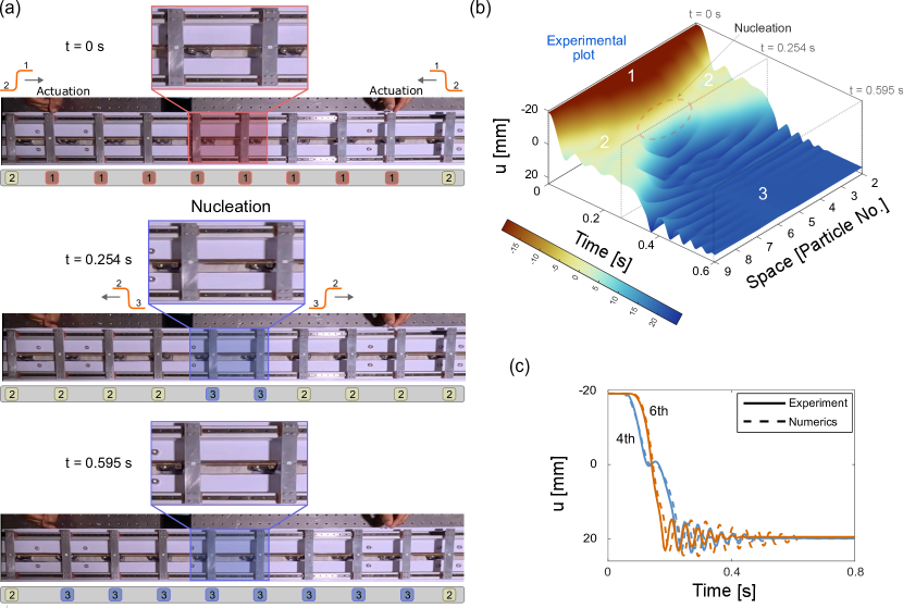
Figure 4: Collision of two $1\rightarrow 2$ transition waves nucleates a new phase, Phase 3. (a) Experimental snapshots highlighting the excitation and nucleation. The unit cells are labeled with the phases. (b) Spatiotemporal plot obtained from experiments showing the nucleation phenomena. The nucleus is formed at the 5th and 6th particles. (c) Displacement time series for the 4th and the 6th particles.

Nucleation

In this section, we study the collision of two transition waves. We consider a chain with an asymmetric tristable onsite potential shown in Fig. 2(b)(i) and excite the chain from both ends. Initially, the entire chain is in Phase 1. We then trigger $1\rightarrow 2$ transition waves from both ends. We observe transition waves propagating towards each other from the extreme ends and colliding at the middle of the chain at about $t=0.254$ s as shown in Fig. 4(a). The collision induces larger displacements and thereby nucleates a new phase, i.e., Phase 3, in the 5th and 6th unit cells. Consequently, this nucleus triggers $2\rightarrow 3$ transition waves from the middle of the chain that propagate back to the boundaries.

In Fig. 4(b), we show experimentally measured spatiotemporal map of displacement. The formation of a remote nucleus and the lattice transforming to Phase 3 is evident. We further show the temporal dynamics of the 4th and 6th unit cells in Fig. 4(c). We observe that the 4th unit cell transitions to Phase 2 ($u\approx 0$) before the 6th unit cell. However, the latter transitions to Phase 3 earlier than the 4th unit cell. This is consistent with the earlier observation that nucleation occurs at the 5th and 6th unit cells.

This phenomenon can be interpreted as the collision of a kink and an anti-kink propagating in opposite directions [33]. After collision, they annihilate and give rise to a new phase. This new phase leads to the formation of a new pair of kink and anti-kink, which propagate in opposite directions. Interestingly, the size of the nucleus depends on the number of particles in the chain. For example, two particles (the 5th and 6th) create the nucleus in the case above. However, for an odd number of particles in the chain, it is possible to have a nucleus of only one particle (see Supplemental Material for details). This implies that even if only a single particle is nucleated due to the collision of a kink and an anti-kink, it can effectively induce the propagation of the new phase in both directions.

Such a collision of two transition waves and triggering remote nucleation of a new phase persists for even longer chains with damping. This is because the asymmetry in the tristable potential well helps overcome the damping effects. Thus, both the colliding and nucleating transition waves are robust for traveling long distances. Moreover, it is also possible to remotely nucleate a new phase at an arbitrary location (and not only at the center) in the chain using a time delay of actuation from either end (see Supplemental Material for details).

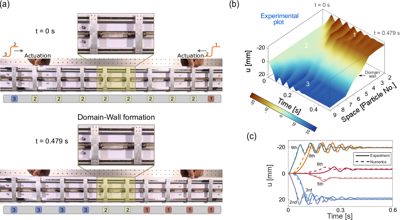
Figure 5: Collision of two transition waves leads to a stationary domain wall. (a) Experimental snapshots highlighting the formation of the stationary domain. The unit cells are labeled with the phases. (b) Spatiotemporal plot obtained from experiments showing the formation of the stationary domain wall. (c) Displacement time series of several particles in the chain.

Stationary Domain Wall

In this section, we investigate the collision of two transition waves but with different onsite potentials. The tunability of our magnetoelastic lattice allows us to obtain a symmetric onsite potential well as shown in Fig. 2(b)(ii). The difference in the energy levels of Phase 2 with Phase 1 and Phase 3 enables two different types of transition waves in the system. Initially, the whole lattice is kept in Phase 2. We trigger $2\rightarrow 1$ and $2\rightarrow 3$ transition waves from opposite ends and observe their collision. This scenario can also be understood as a collision of two kinks [33].

In Fig. 5(a), we observe two distinct propagating transition waves (moving domain walls) that collide at the center of the chain. However, the 5th and the 6th particles in the chain continue to remain in Phase 2, forming a stationary domain wall between Phase 1 and Phase 3. In Fig. 5(b), we show experimentally measured spatiotemporal maps of displacement confirming the formation of a stationary domain wall.

In Fig. 5(c), we plot the transient response of several particles in the chain. We observe that the 5th and the 6th particles remain stationary, forming a stationary domain wall; however, their equilibrium state is slightly perturbed from Phase 2 due to the coexistence of other states next to them.

We also verify that stationary domain walls can form in longer chains. Moreover, the domain wall could be made of only one particle if the chain consists of an odd number of particles. Finally, the location of the domain wall can be tuned by introducing a time delay in triggering the transition waves from opposite ends (refer to Supplementary Material for details).

Conclusion

In summary, we investigate a one-dimensional magnetoelastic chain with tunable onsite potential. Specifically, our focus is on a tristable lattice, where we experimentally verify the existence of different types of transition waves. These waves robustly propagate in the lattice due to the designed asymmetry in the potential well. We also verify experimentally a scaling law that relates the averaged power dissipated to the asymmetry in the potential well and wave velocity for all types of transition waves.

Additionally, we explore the collision of transition waves. In the case of an asymmetric potential well, when two transition waves collide as a kink and anti-kink, we observe the remote nucleation of a new phase. However, in the case of a symmetric potential well, two transition waves collide as kinks, resulting in the formation of a stationary domain wall between two different phases.

These findings underscore the richness of dynamical phenomena in multistable lattices. The design holds promise for the development of reconfigurable materials under external fields, where remote actuation through transition waves can be utilized to tune the final state of the material.

Supplemental Material

I Calculation of onsite potential

A uniform magnetized sphere B, supporting a magnetization $\textbf{m}(\textbf{x})$ generates a magnetic field $\textbf{h}(\textbf{x})$ on all $R^{3}$. The magnetic field $\textbf{h}(\textbf{x})$ can be obtained by solving Maxwell’s equation of magnetization:

$$\begin{split}\begin{aligned} \nabla\times\mathbf{h}(\textbf{x})&=0,\\ \nabla\cdot(\mathbf{h}(\textbf{x})+\mathbf{m}\,\chi_{{}_{B}})&=0,\end{aligned}\end{split}$$ (1)

where $\chi_{{}_{B}}$ is the characteristic function defined as follows:

$$\chi_{{}_{B}}=\begin{cases}1&\text{for }\mathbf{x}\in B\\ 0&\text{for }\mathbf{x}\in R^{3}\texttt{\textbackslash}B\,.\end{cases}$$ (2)

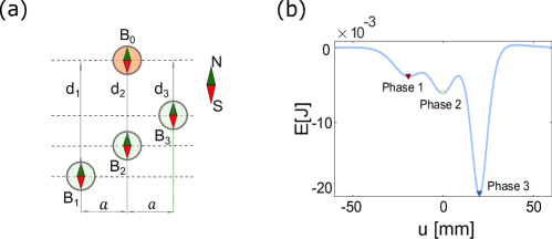
Figure S1: (a) Schematic of the unit cell, where the fixed magnets are kept at depths $d_{1}$, $d_{2}$ and $d_{3}$ from the the moving magnet. (c) Onsite potential of tristable unit cell.

For a uniformly magnetized sphere, the induced magnetic field $\textbf{h}(\textbf{x})$ is given as [34]

$$\textbf{h}(\textbf{x})=\begin{cases}-\dfrac{1}{3}\mathcal{I}\textbf{m}&\text{for }\mathbf{x}\leq B\\[20.00003pt] -\dfrac{r^{3}}{3}\left(\dfrac{\mathcal{I}}{|\mathbf{x}|^{3}}-3\dfrac{\mathbf{x}\otimes\mathbf{x}}{|\mathbf{x}|^{5}}\right)\textbf{m}&\text{for }\mathbf{x}\geq B\,.\end{cases}$$ (3)

The magnetostatic energy of a uniformly magnetized sphere can be computed as follows

$$ME=k_{d}\int_{R^{3}}|\mathbf{h}|^{2}\,\mathbf{dx}=-k_{d}\int_{R^{3}}\mathbf{h}.\mathbf{m}\,\mathbf{dx}=-k_{d}\int_{B}\mathbf{h}.\mathbf{m}\,\mathbf{dx}=-k_{d}\mathbf{m}.\int_{B}\mathbf{h}\,\mathbf{dx}=k_{d}\mathbf{m}.\dfrac{\mathcal{I}}{3}\mathbf{m}|B|$$ (4)

where $k_{d}=m_{s}^{2}/2\mu_{0}$, $m_{s}$ being the magnetization of the uniformly magnetized sphere, $\mu_{0}=4\pi\times 10^{-7}\,\text{Vs/Am}$ denotes vacuum permeability and $|B|$ denotes the volume of the sphere

We now write down the total magnetostatic energy of four uniformly magnetized identical spheres $B_{0}$, $B_{1}$, $B_{2}$, and $B_{3}$ (see Fig. S1(a)) supporting magnetization $\mathbf{m}_{0}$, $\mathbf{m}_{1}$, $\mathbf{m}_{2}$ and $\mathbf{m}_{3}$ respectively, as

$$\begin{split}ME&=k_{d}\int_{R^{3}}|\mathbf{h}_{0}+\mathbf{h}_{1}+\mathbf{h}_{2}+\mathbf{h}_{3}|^{2}\mathbf{dx}\\ &=\underbrace{k_{d}\left(\int_{R^{3}}{h_{0}}^{2}\mathbf{dx}+\int_{R^{3}}{h_{1}}^{2}+\mathbf{dx}\int_{R^{3}}{h_{2}}^{2}\mathbf{dx}+\int_{R^{3}}{h_{3}}^{2}\mathbf{dx}\right)}_{\text{self-energies}}+\\ &\quad\underbrace{2k_{d}\left(\int_{R^{3}}\mathbf{h}_{0}.\mathbf{h}_{1}\,\mathbf{dx}+\int_{R^{3}}\mathbf{h}_{0}.\mathbf{h}_{2}\,\mathbf{dx}+\int_{R^{3}}\mathbf{h}_{0}.\mathbf{h}_{3}\,\mathbf{dx}+\int_{R^{3}}\mathbf{h}_{1}.\mathbf{h}_{2}\,\mathbf{dx}\right.+\left.\int_{R^{3}}\mathbf{h}_{1}.\mathbf{h}_{3}\,\mathbf{dx}+\int_{R^{3}}\mathbf{h}_{2}.\mathbf{h}_{3}\,\mathbf{dx}\right)}_{\text{interaction energies}}\,.\end{split}$$ (5)

The first four integrals represent the self energies and the last six integrals represent the interaction energies. Note that the interaction energy is of the form $\int\mathbf{h}_{i}.\mathbf{h}_{j}\,\mathbf{dx}$ and represents the interaction energy of the $i^{th}$ magnet and the $j^{th}$ magnet ($i\neq j$). This interaction energy depends on the distance between the $i^{th}$ magnet and the $j^{th}$ magnet.

Since $B_{1}$, $B_{2}$ and $B_{3}$ are fixed and uniformly magnetized spheres; $\int\mathbf{h}_{1}.\mathbf{h}_{2}\,\mathbf{dx}$, $\int\mathbf{h}_{1}.\mathbf{h}_{3}\,\mathbf{dx}$ and $\int\mathbf{h}_{2}.\mathbf{h}_{3}\,\mathbf{dx}$ are all constants. Also note that since $B_{1}$, $B_{2}$ and $B_{3}$ are uniformly magnetized, their self energies (see Eq. (4)) can be written as

$$\int_{R^{3}}{h_{0}}^{2}\mathbf{dx}=\int_{R^{3}}{h_{1}}^{2}=\mathbf{dx}\int_{R^{3}}{h_{2}}^{2}\mathbf{dx}=\int_{R^{3}}{h_{3}}^{2}\mathbf{dx}=k_{d}\mathbf{m}.\dfrac{\mathcal{I}}{3}\mathbf{m}|B|=constant\,.$$ (6)

Evaluation of the integral in Eq. (5) yields the total magnetostatic energy of the system as follows

$$ME=\underbrace{2k_{d}\left(\int_{R^{3}}\mathbf{h}_{0}.\mathbf{h}_{1}\,\mathbf{dx}+\int_{R^{3}}\mathbf{h}_{0}.\mathbf{h}_{2}\,\mathbf{dx}+\int_{R^{3}}\mathbf{h}_{0}.\mathbf{h}_{3}\mathbf{dx}\right)}_{\text{interaction energies}}+constant\,.$$ (7)

We thus get the total magnetostatic energy (modulo a constant) as

$$\begin{split}E&=2k_{d}\left(\int_{R^{3}}\mathbf{h}_{0}.\mathbf{h}_{1}\,\mathbf{dx}+\int_{R^{3}}\mathbf{h}_{0}.\mathbf{h}_{2}\,\mathbf{dx}+\int_{R^{3}}\mathbf{h}_{0}.\mathbf{h}_{3}\mathbf{dx}\right)\,.\end{split}$$ (8)

For the considered unit cell with three fixed magnets spaced at a distance $a$ (i.e., their centers are located at $x=-a,\,0,\,a$) at depths $d_{1}$, $d_{2}$ and $d_{3}$ from the moving magnet (see Fig.  S1(a)), we can evaluate the above integral and obtain the following:

$$\begin{split}E(u,a,d_{1},d_{2},d_{3})=&\frac{4\pi m_{s}^{2}}{9\mu_{0}}r^{6}\Bigg{[}\Bigg{(}\frac{1}{((u+a)^{2}+d_{1}^{2})^{\frac{3}{2}}}-\frac{3d_{1}^{2}}{((u+a)^{2}+d_{1}^{2})^{\frac{5}{2}}}\Bigg{)}+\left(\frac{1}{(u^{2}+d_{2}^{2})^{\frac{3}{2}}}-\frac{3d_{2}^{2}}{(u^{2}+d_{2}^{2})^{\frac{5}{2}}}\right)\\ &+\left(\frac{1}{((u-a)^{2}+d_{3}^{2})^{\frac{3}{2}}}-\frac{3d_{3}^{2}}{((u-a)^{2}+d_{3}^{2})^{\frac{5}{2}}}\right)\Bigg{]}.\end{split}$$ (9)

The exact energy is plotted in Fig. S1(b), with numerical values: $\mu_{0}=4\pi\times 10^{-7}\,\text{Vs/Am}$, $m_{s}=0.8\,\text{T}$, $(d_{1},d_{2},d_{3})=(18,15.3,10.4)$ mm, $r=5$ mm and $a=20$ mm. Therefore, we achieve a tristable onsite energy potential, and define the three stable states as Phase 1, Phase 2, and Phase 3. The tunable depths $d_{1}$, $d_{2}$ and $d_{3}$ help us to tailor the energy landscape.

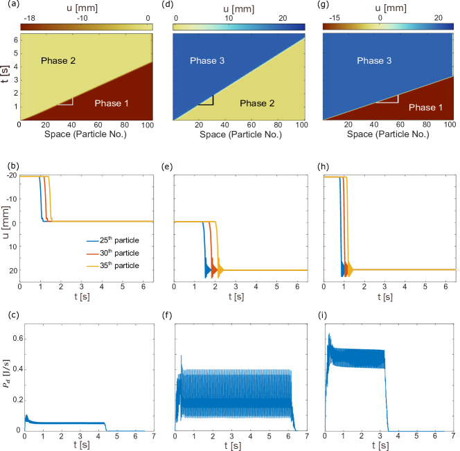
Figure S2: Numerical study for a chain of 100 particles. (a) (d) (g) Spatiotemporal plot of displacement (b) (e) (h) displacement-time series, and (c) (f) (i) Dissipated power, for (a) (b) (c) $1\rightarrow 2$ transition, (d) (e) (f) $2\rightarrow 3$ transition, (g) (h) (i) $1\rightarrow 3$ transition.

II Transition waves in longer chains with damping

Considering the system parameters used in experiments, we conduct numerical simulations on longer chains consisting of 100 particles. With similar initial conditions as described in the main text, we observe that all $1\rightarrow 2$, $2\rightarrow 3$, and $1\rightarrow 3$ transition waves are sustainable even in longer chains, as shown in Fig. S2.

We also calculate the dissipated power $(P_{d})$ for all three transitions. It is notable that the dissipated power oscillates in time with a period $T=l/\nu$. We compute the time-averaged $P_{d}$ and utilize it to verify the scaling law (Eq. 11) numerically and experimentally (as seen in Fig. 3(e) in the manuscript).

III Reflection of transition waves from a free boundary

We investigate a chain of 100 unit cells with the tristable asymmetric onsite potential depicted in Fig. 2(b) of the main text. Unlike previously, the right end of the chain is kept free instead of fixed. Initially, all unit cells in the chain are in Phase 1. The first element is forced to snap to Phase 2.

In Fig. S3, we observe a $1\rightarrow 2$ transition wave traveling from left to right, converting the entire chain to Phase 2. Upon reaching the right (free) boundary, a new transition wave ($2\rightarrow 3$) reflects back, converting the entire chain from Phase 2 to Phase 3 (the lowest energy state).

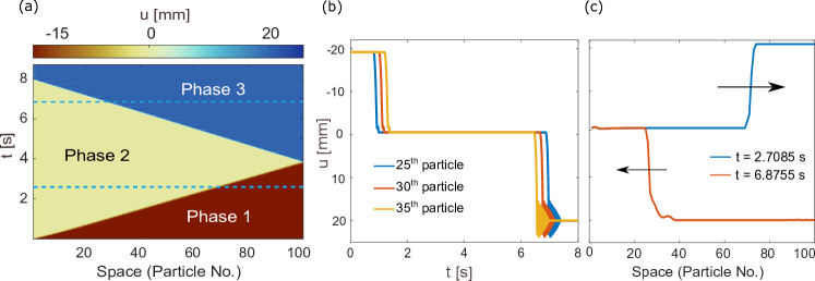
Figure S3: Reflection of transition wave from a free boundary. (a) Spatiotemporal plot of displacement, (b) displacement-time series, (c) spatial profiles at time 2.7085 s and 6.8755 s

IV Nucleation in longer chains with damping

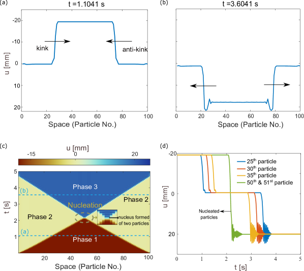
Figure S4: Collision of a kink and and an anti-kink resulting in the formation of a new phase in longer chains. (a)-(b) spatial profiles at time 1.1041 s and 3.6041 s respectively. (c) Spatiotemporal plot of displacement for the formation of a Phase 3 upon collision of two transition fronts $1\rightarrow 2$, (d) displacement-time series.

We investigate longer chains comprising 100 unit cells for nucleation study. Initially, all unit cells are in Phase 1. $1\rightarrow 2$ transition waves are triggered from opposite ends. Despite damping, these waves persist in longer chains, as shown in Fig. S4(a). The collision of the kink and anti-kink occurs at the center, leading to their annihilation and the emergence of a new phase (Phase 3). This new phase initiates the formation of a new pair of kink and anti-kink, propagating in opposite directions as $2\rightarrow 3$ transition waves shown in Fig. S4(b). Thus, the current configuration, with asymmetric potentials and the collision dynamics of kink and anti-kink, presents a robust method for remotely nucleating a new phase even in longer chains and damped systems.

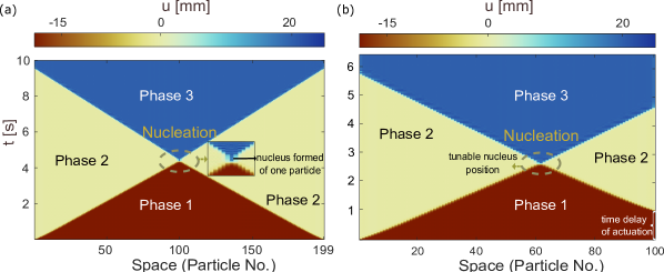
Figure S5: Nucleation observed when lattice is made up of odd number of unit cells (199 particles). (a) Spatiotemporal plot of displacement for 199 particles. Tunable spatial location of nucleation using time delay of actuation, (b) spatiotemporal plot of displacement when the right end of the chain is actuated at delay of 1 s.

Note that the nucleus of the new phase shown in Figs. S4(c),(d) consists of the two middlemost particles in chains with an even number of unit cells. However, for an odd number of particles ($n=199$) in the chain, the collision of a kink and anti-kink from either side of the chain results in only the central (singular) element acquiring Phase 3. The nucleus formed by this single element (the 100th particle) effectively initiates the propagation of the new phase in both directions of the chain, as shown in Fig. S5(a).

Moreover, we can tailor the spatial location of nucleation using a time delay of actuation from either end, as demonstrated in Fig. S5(b). We consider a chain consisting of 100 unit cells. We apply similar initial conditions at both ends (Phase 1 to Phase 3), but the right end of the chain is actuated with a delay of 1 s. Consequently, a nucleus is formed upon the collision of two waves, but not precisely at the center of the chain. Instead, the nucleus is biased towards the right end of the chain. Nonetheless, this nucleus can effectively trigger $2\rightarrow 3$ transition waves in both directions of the chain. Hence, the time-delayed actuation from either end provides a convenient method to tailor the spatial location of remote nucleation within the lattice.

V Stationary domain walls in longer chains with damping

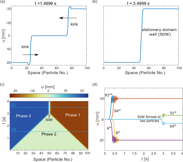
Figure S6: Collision of two kinks resulting in a stationary domain wall in longer chains. (a)-(b) spatial profiles at time 1.4999 s and 3.4999 s respectively. (c) spatiotemporal plot of dsplacement and (d) displacement time series, for the case when the chain is constituted of even (100) number of particles. The stationary domain wall is formed of two unit cells.

We perform numerical simulations on longer chains of length 100 (and 99) with opposite initial conditions, i.e. we trigger $2\rightarrow 3$ and $2\rightarrow 1$ transition waves from opposite ends. Upon collision of two kinks, we clearly observe the formation of domain wall in both the cases as shown in Figs. S6 and S7. It is intriguing to note that in odd chain lengths, a single particle forms the stationary domain wall, while in even chain lengths, the stationary domain wall is shared by two particles. Note that the steady state of the stationary domain wall is different in odd and even number of particles. When we have a chain made of odd number of unit cells, the stationary domain wall remains exactly at Phase 2 $(u\approx 0)$, as shown in Fig. S7(b). However, when the number of elements in the chain is even, the domain wall is shared by the middlemost two elements, having their equilibrium state slightly perturbed from Phase 2, as shown in Fig. S6(d).

Furthermore, by adjusting the timing of actuation from each end, as illustrated in Fig. S8, we can customize the spatial position of the stationary domain wall. We examine a chain comprising 100 unit cells. While triggering $2\rightarrow 1$ and $2\rightarrow 3$ transition waves from opposite ends, we introduce a 1-second delay in actuation at the right end of the chain. Consequently, upon the collision of these waves, a stationary domain wall forms, not exactly at the chain’s center. Instead, it biases towards the right end. Thus, employing time-delayed actuation from either end offers a convenient means to adjust the spatial location of stationary domain wall within the lattice.

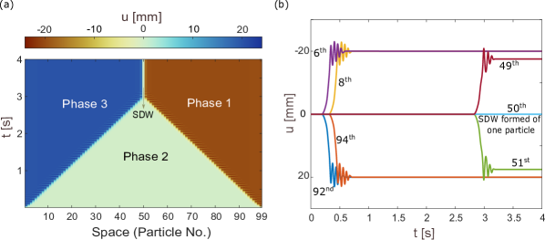
Figure S7: Formation of domain walls in case of odd number of particles (a) spatiotemporal plot of displacement and (b) displacement time series for the case when the chain is constituted of odd (99) number of particles. The stationary domain wall is formed of one unit cell.

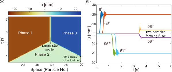
Figure S8: Spatially tunable domain wall. The right end of the chain is actuated at a delay of 1 s. (a) spatiotemporal plot of displacement and (b) displacement time series of 100 particles. The SDW is formed of 58th and 59th particle.

References

- Braun and Kivshar [2004] O. M. Braun and Y. S. Kivshar, The Frenkel-Kontorova model: concepts, methods, and applications (Springer, 2004).
- Currie et al. [1979] J. F. Currie, A. Blumen, M. A. Collins, and J. Ross, Dynamics of domain walls in ferrodistortive materials ii. applications to - and sbsi-type ferroelectrics, Phys. Rev. B 19, 3645 (1979).
- Atkinson et al. [2003] D. Atkinson, D. A. Allwood, G. Xiong, M. D. Cooke, C. C. Faulkner, and R. P. Cowburn, Magnetic domain-wall dynamics in a submicrometre ferromagnetic structure, Nature Materials 2003 2:2 2, 85 (2003).
- Falk [1984] F. Falk, Ginzburg-landau theory and solitary waves in shape-memory alloys, Zeitschrift für Physik B Condensed Matter 54, 159 (1984).
- Remoissenet and Peyrard [1984] M. Remoissenet and M. Peyrard, Soliton dynamics in new models with parametrized periodic double-well and asymmetric substrate potentials, Physical Review B 29, 3153 (1984).
- Pouget and Maugin [1985] J. Pouget and G. A. Maugin, Solitons and electroacoustic interactions in ferroelectric crystals. ii. interactions of solitons and radiations, Physical Review B 31, 4633 (1985).
- Abeyaratne and Knowles [1991] R. Abeyaratne and J. K. Knowles, Kinetic relations and the propagation of phase boundaries in solids, Archive for Rational Mechanics and Analysis 114, 119 (1991).
- Peyrard [1998] M. Peyrard, Simple theories of complex lattices, Physica D: Nonlinear Phenomena 123, 403 (1998).
- Flach et al. [1999] S. Flach, Y. Zolotaryuk, and K. Kladko, Moving lattice kinks and pulses: An inverse method, Physical Review E 59, 6105 (1999).
- Slepyan and Ayzenberg-Stepanenko [2004] L. Slepyan and M. Ayzenberg-Stepanenko, Localized transition waves in bistable-bond lattices, Journal of the Mechanics and Physics of Solids 52, 1447 (2004).
- Slepyan et al. [2005] L. Slepyan, A. Cherkaev, and E. Cherkaev, Transition waves in bistable structures. ii. analytical solution: wave speed and energy dissipation, Journal of the Mechanics and Physics of Solids 53, 407 (2005).
- Truskinovsky and Vainchtein [2005] L. Truskinovsky and A. Vainchtein, Kinetics of martensitic phase transitions: lattice model, SIAM Journal on Applied Mathematics 66, 533 (2005).
- Benichou and Givli [2013] I. Benichou and S. Givli, Structures undergoing discrete phase transformation, Journal of the Mechanics and Physics of Solids 61, 94 (2013).
- Nadkarni et al. [2016a] N. Nadkarni, A. F. Arrieta, C. Chong, D. M. Kochmann, and C. Daraio, Unidirectional transition waves in bistable lattices, Physical review letters 116, 244501 (2016a).
- Deng et al. [2021] B. Deng, J. R. Raney, K. Bertoldi, and V. Tournat, Nonlinear waves in flexible mechanical metamaterials, Journal of Applied Physics 130, 40901 (2021).
- Deng et al. [2020a] B. Deng, L. Chen, D. Wei, V. Tournat, and K. Bertoldi, Pulse-driven robot: Motion via solitary waves, Science Advances 6 (2020a).
- Chi et al. [2022] Y. Chi, Y. Li, Y. Zhao, Y. Hong, Y. Tang, J. Yin, Y. Chi, Y. Li, Y. Zhao, Y. Hong, J. Yin, and Y. Tang, Bistable and multistable actuators for soft robots: Structures, materials, and functionalities, Advanced Materials 34, 2110384 (2022).
- Shan et al. [2015] S. Shan, S. H. Kang, J. R. Raney, P. Wang, L. Fang, F. Candido, J. A. Lewis, K. Bertoldi, S. Shan, S. H. Kang, J. R. Raney, P. Wang, L. Fang, F. Candido, J. A. Lewis, and K. Bertoldi, Multistable architected materials for trapping elastic strain energy, Advanced Materials 27, 4296 (2015).
- Zareei et al. [2020] A. Zareei, B. Deng, and K. Bertoldi, Harnessing transition waves to realize deployable structures, Proceedings of the National Academy of Sciences of the United States of America 117, 4015 (2020).
- Ramakrishnan et al. [2020] V. Ramakrishnan, . M. J. Frazier, and M. J. Frazier, Multistable metamaterial on elastic foundation enables tunable morphology for elastic wave control, Journal of Applied Physics 127, 225104 (2020).
- Watkins et al. [2021] A. A. Watkins, A. Eichelberg, and O. R. Bilal, Exploiting localized transition waves to tune sound propagation in soft materials, Physical Review B 104, L140101 (2021).
- Nadkarni et al. [2014] N. Nadkarni, C. Daraio, and D. M. Kochmann, Dynamics of periodic mechanical structures containing bistable elastic elements: From elastic to solitary wave propagation, Physical Review E 90, 023204 (2014).
- Katz and Givli [2018] S. Katz and S. Givli, Solitary waves in a bistable lattice, Extreme Mechanics Letters 22, 106 (2018).
- Shiroky and Gendelman [2018] I. Shiroky and O. Gendelman, Propagation of transition fronts in nonlinear chains with non-degenerate on-site potentials, Chaos: An Interdisciplinary Journal of Nonlinear Science 28 (2018).
- Deng et al. [2020b] B. Deng, P. Wang, V. Tournat, and K. Bertoldi, Nonlinear transition waves in free-standing bistable chains, Journal of the Mechanics and Physics of Solids 136, 103661 (2020b).
- Pal and Sitti [2023] A. Pal and M. Sitti, Programmable mechanical devices through magnetically tunable bistable elements, Proceedings of the National Academy of Sciences 120, e2212489120 (2023).
- ZhouWang [2023] W.-Z. ZhouWang, Cooperative propagation and directional phase transition of topological solitons in multi-stable mechanical metamaterials, Journal of the Mechanics and Physics of Solids , 105287 (2023).
- Yasuda et al. [2020] H. Yasuda, L. Korpas, and J. Raney, Transition waves and formation of domain walls in multistable mechanical metamaterials, Physical Review Applied 13, 054067 (2020).
- Yasuda et al. [2023] H. Yasuda, H. Shu, W. Jiao, V. Tournat, and J. R. Raney, Nucleation of transition waves via collisions of elastic vector solitons, Applied Physics Letters 123 (2023).
- Jin et al. [2020] L. Jin, R. Khajehtourian, J. Mueller, A. Rafsanjani, V. Tournat, K. Bertoldi, and D. M. Kochmann, Guided transition waves in multistable mechanical metamaterials, Proceedings of the National Academy of Sciences 117, 2319 (2020).
- Deng et al. [2020c] B. Deng, S. Yu, A. E. Forte, V. Tournat, and K. Bertoldi, Characterization, stability, and application of domain walls in flexible mechanical metamaterials, Proceedings of the National Academy of Sciences 117, 31002 (2020c).
- Nadkarni et al. [2016b] N. Nadkarni, C. Daraio, R. Abeyaratne, and D. M. Kochmann, Universal energy transport law for dissipative and diffusive phase transitions, Physical Review B 93, 104109 (2016b).
- Remoissenet [2013] M. Remoissenet, Waves called solitons: concepts and experiments (Springer Science & Business Media, 2013).
- James and Müller [1994] R. D. James and S. Müller, Internal variables and fine-scale oscillations in micromagnetics, Continuum Mechanics and Thermodynamics 6, 291 (1994).